Lecture # 14Lecture # 14

Perfectly Competitive Perfectly Competitive MarketsMarkets

Lecturer: Martin ParedesLecturer: Martin Paredes

2

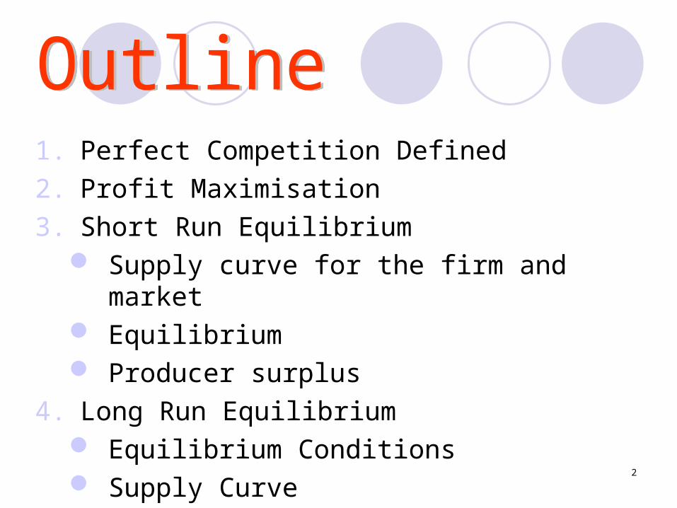
1. Perfect Competition Defined2. Profit Maximisation3. Short Run Equilibrium

Supply curve for the firm and market Equilibrium Producer surplus

4. Long Run Equilibrium Equilibrium Conditions Supply Curve

3

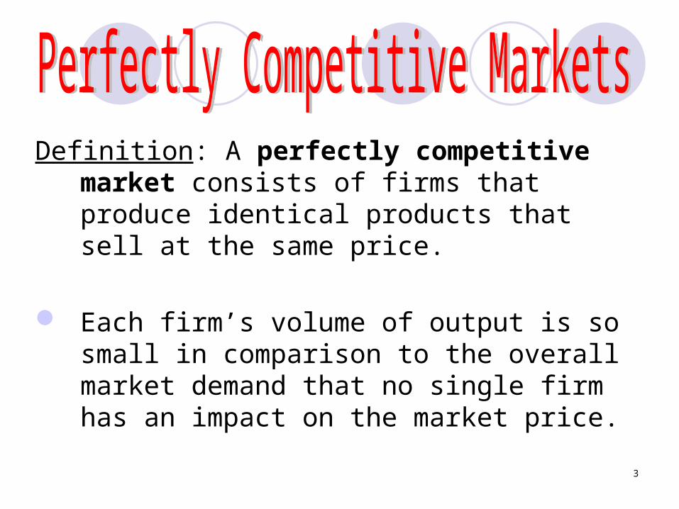
Definition: A perfectly competitive market consists of firms that produce identical products that sell at the same price.

Each firm’s volume of output is so small in comparison to the overall market demand that no single firm has an impact on the market price.

4

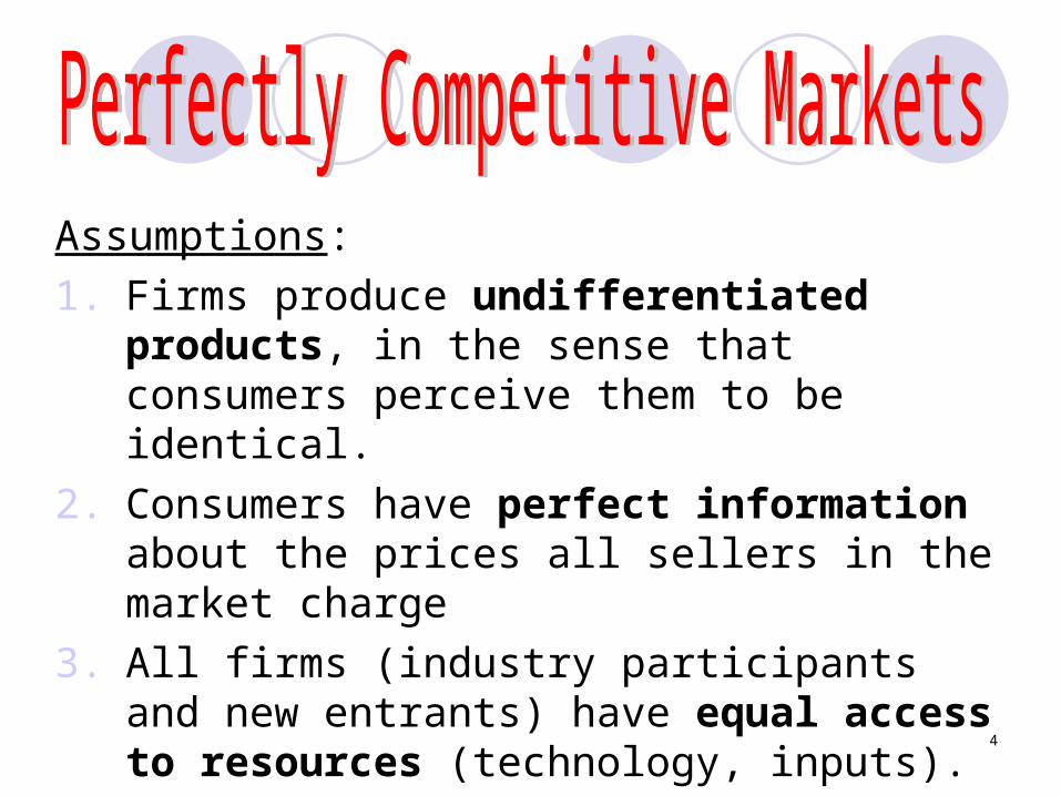
Assumptions: 1. Firms produce undifferentiated

products, in the sense that consumers perceive them to be identical.

2. Consumers have perfect information about the prices all sellers in the market charge

3. All firms (industry participants and new entrants) have equal access to resources (technology, inputs).

5

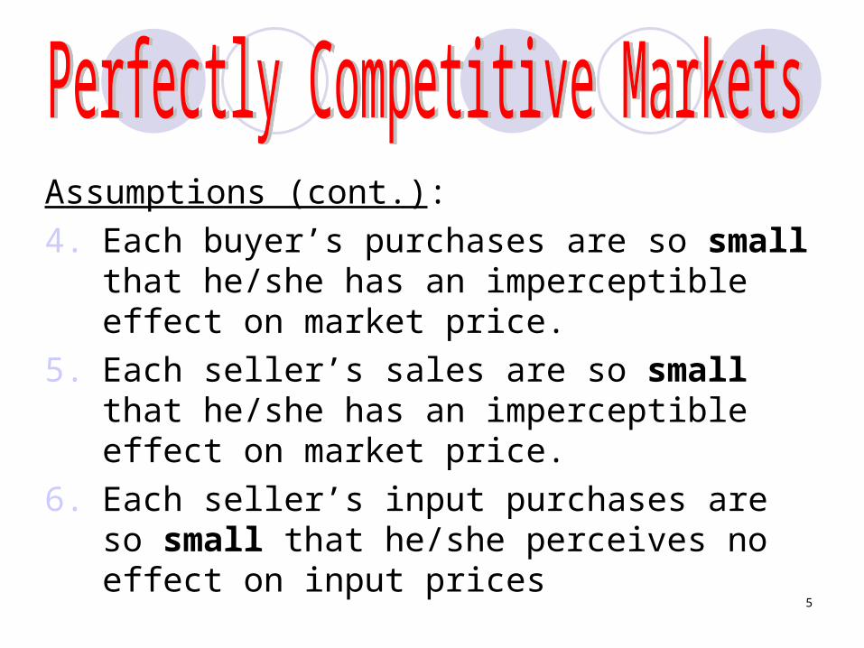
Assumptions (cont.): 4. Each buyer’s purchases are so small that

he/she has an imperceptible effect on market price.

5. Each seller’s sales are so small that he/she has an imperceptible effect on market price.

6. Each seller’s input purchases are so small that he/she perceives no effect on input prices

6

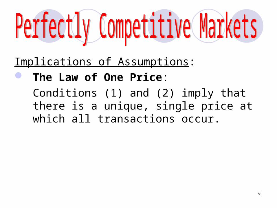
Implications of Assumptions: The Law of One Price:

Conditions (1) and (2) imply that there is a unique, single price at which all transactions occur.

7

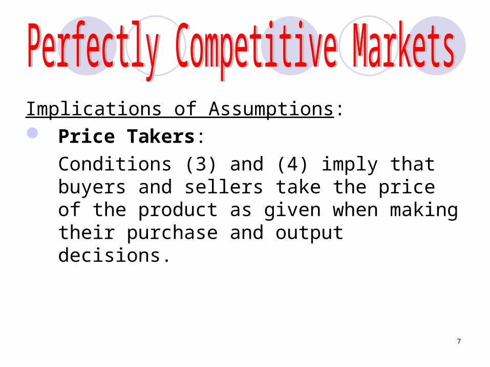
Implications of Assumptions: Price Takers:

Conditions (3) and (4) imply that buyers and sellers take the price of the product as given when making their purchase and output decisions.

8

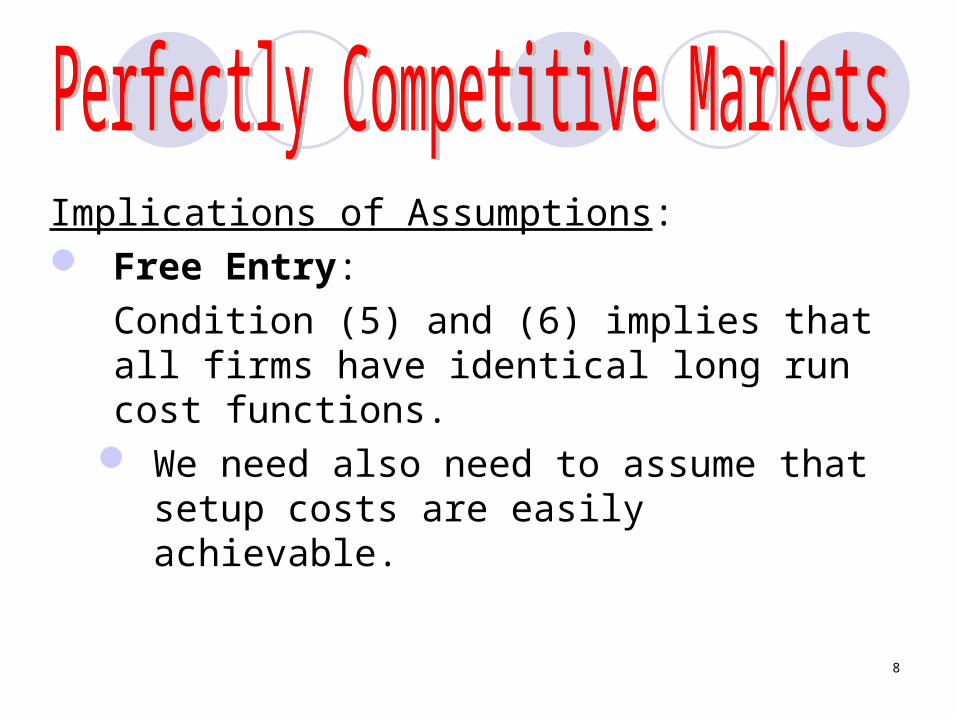
Implications of Assumptions: Free Entry:

Condition (5) and (6) implies that all firms have identical long run cost functions.

We need also need to assume that setup costs are easily achievable.

9

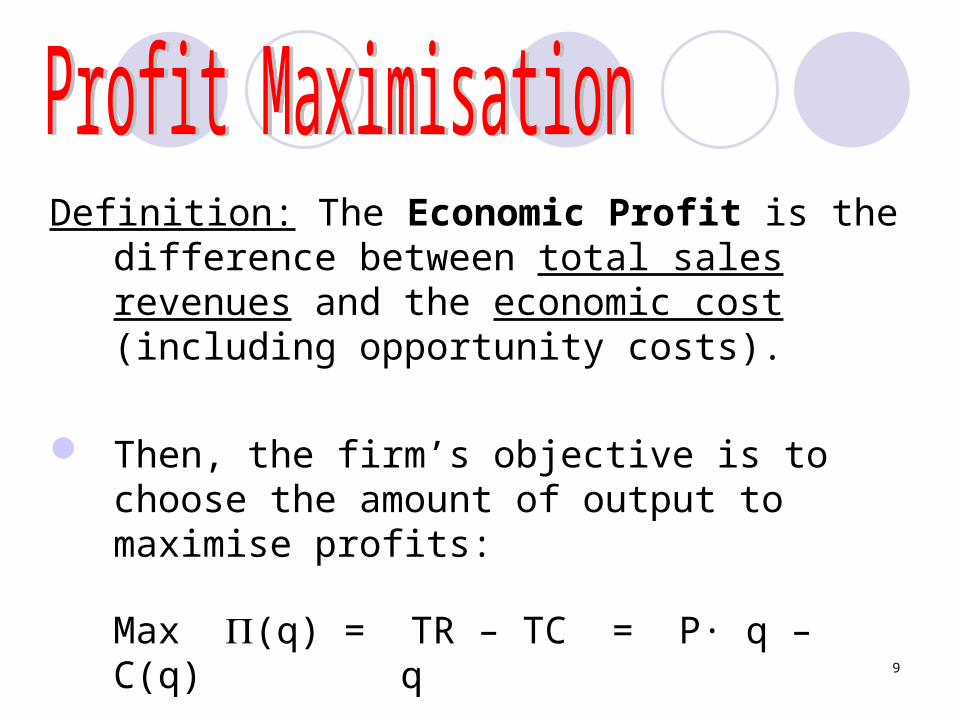
Definition: The Economic Profit is the difference between total sales revenues and the economic cost (including opportunity costs).

Then, the firm’s objective is to choose the amount of output to maximise profits:

Max (q) = TR – TC = P· q – C(q)q

10

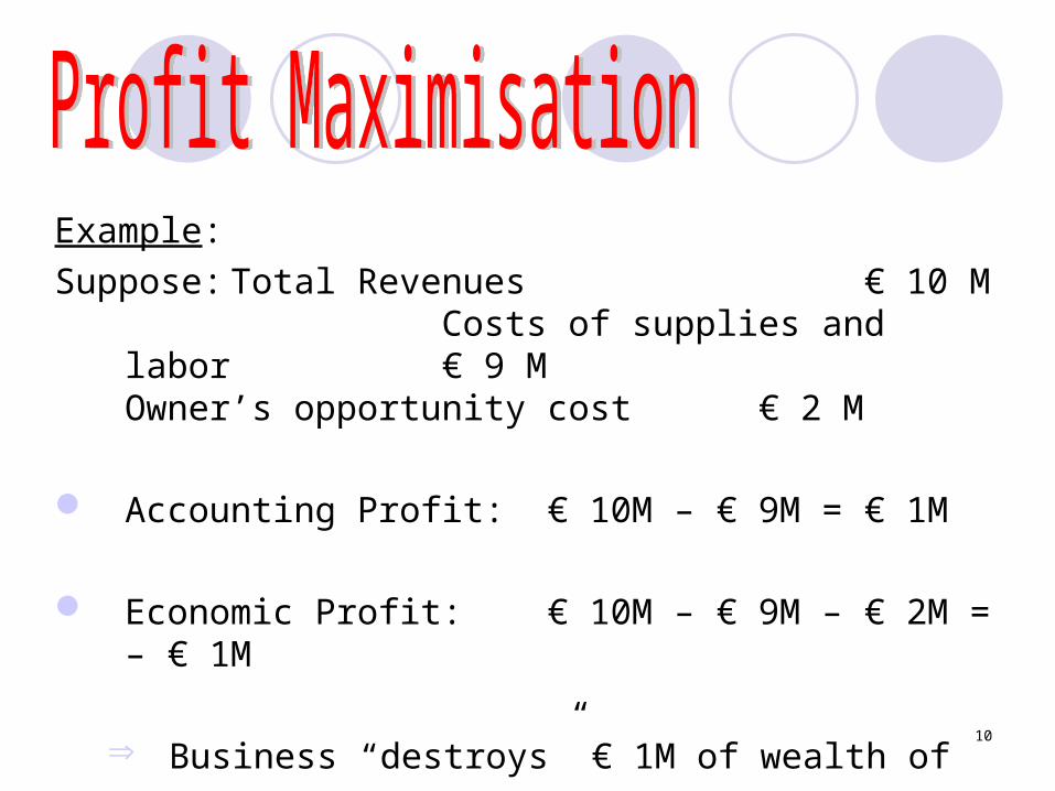
Example:Suppose: Total Revenues € 10 M

Costs of supplies and labor € 9 M Owner’s opportunity cost

€ 2 M

Accounting Profit: € 10M – € 9M = € 1M

Economic Profit: € 10M – € 9M – € 2M = – € 1M

Business “destroys” € 1M of wealth of owner

11

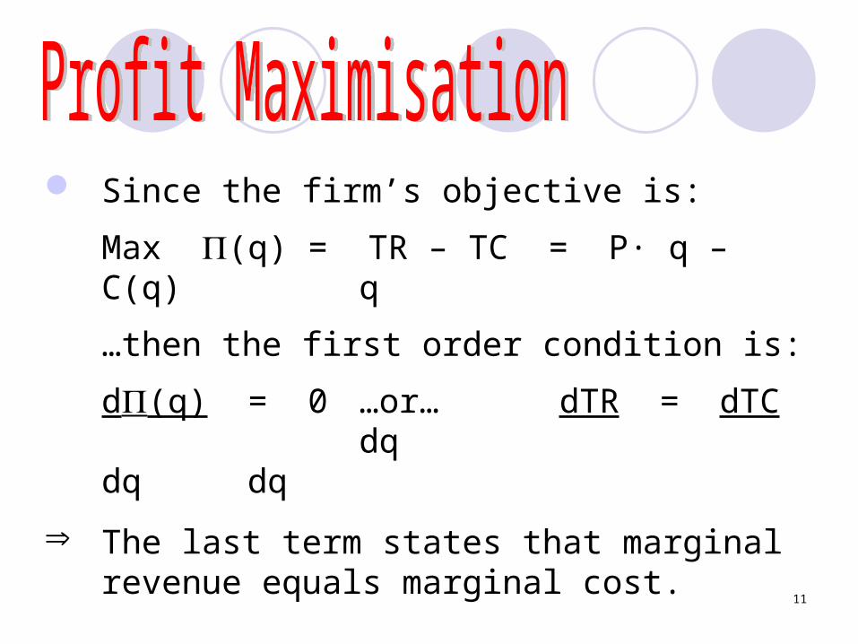
Since the firm’s objective is:

Max (q) = TR – TC = P· q – C(q)q

…then the first order condition is:

d(q) = 0 …or… dTR = dTC dq dq dq

The last term states that marginal revenue equals marginal cost.

12

Notes: Recall that: If MR > MC then profit rises if output is

increased => Increase output. If MR < MC then profit falls if output is

increased => Decrease output. Therefore, the profit maximization

condition for any firm is MR = MC.

13

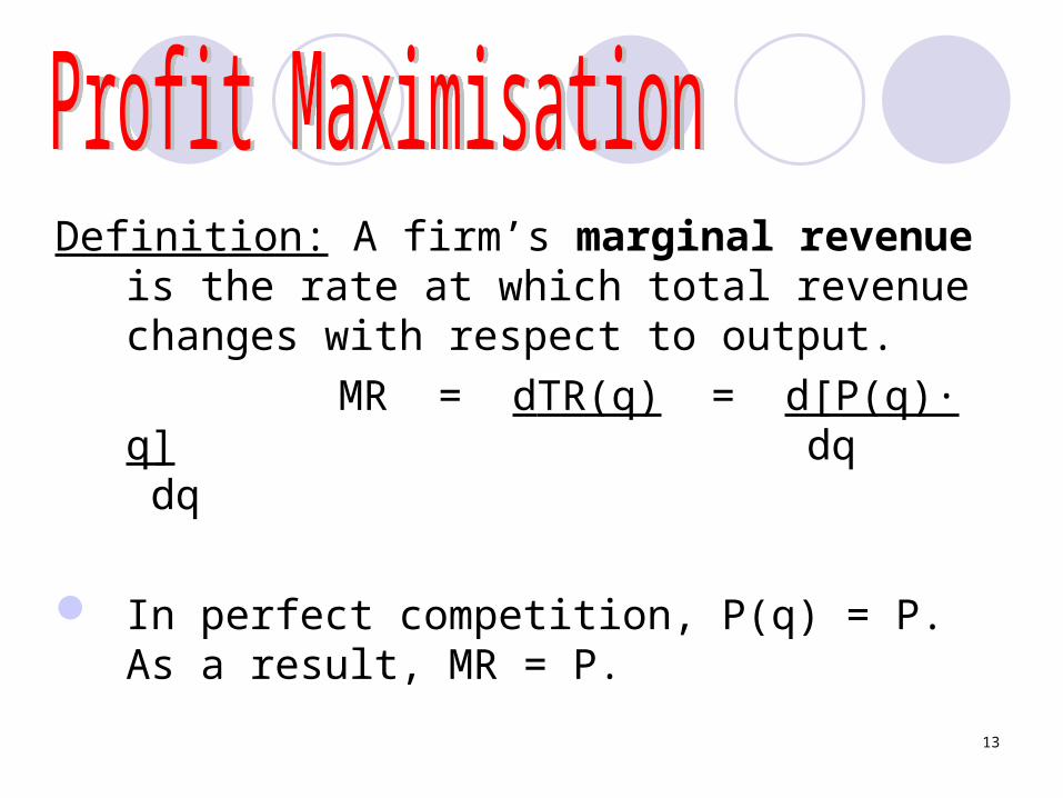
Definition: A firm’s marginal revenue is the rate at which total revenue changes with respect to output.

MR = dTR(q) = d[P(q)· q] dq dq

In perfect competition, P(q) = P. As a result, MR = P.

14

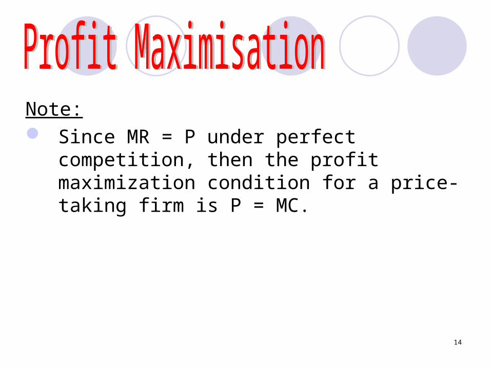
Note: Since MR = P under perfect competition,

then the profit maximization condition for a price-taking firm is P = MC.

15

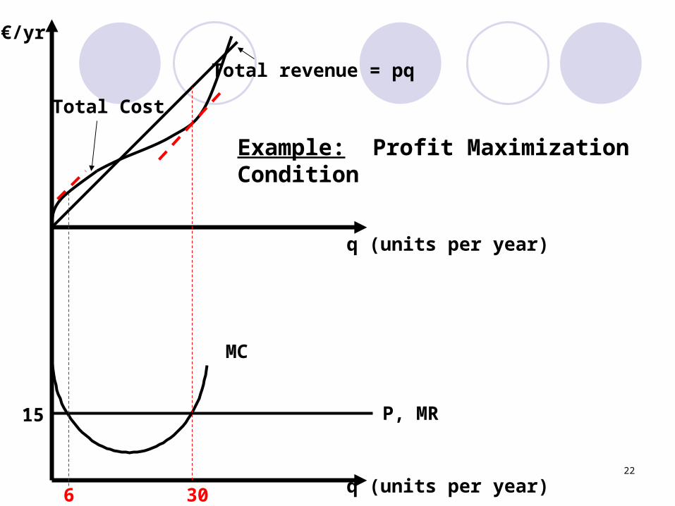
Example:Suppose:

The market price is P = 15 Each firm has the cost function:

TC(q) = 24q – 0.9q2 + 0.0167q3

=> MC(q) = 24 – 1.8q + 0.05q2

16

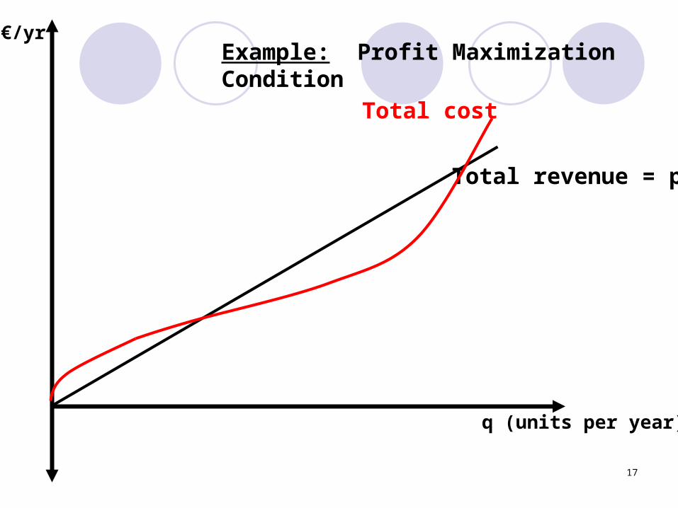
Example: Profit Maximization Condition

€/yr

q (units per year)

Total revenue = pq

15

17

Example: Profit Maximization Condition

€/yr

q (units per year)

Total revenue = pq

Total cost

18

Example: Profit Maximization Condition

€/yr

q (units per year)

Total revenue = pq

Total cost

Total profit

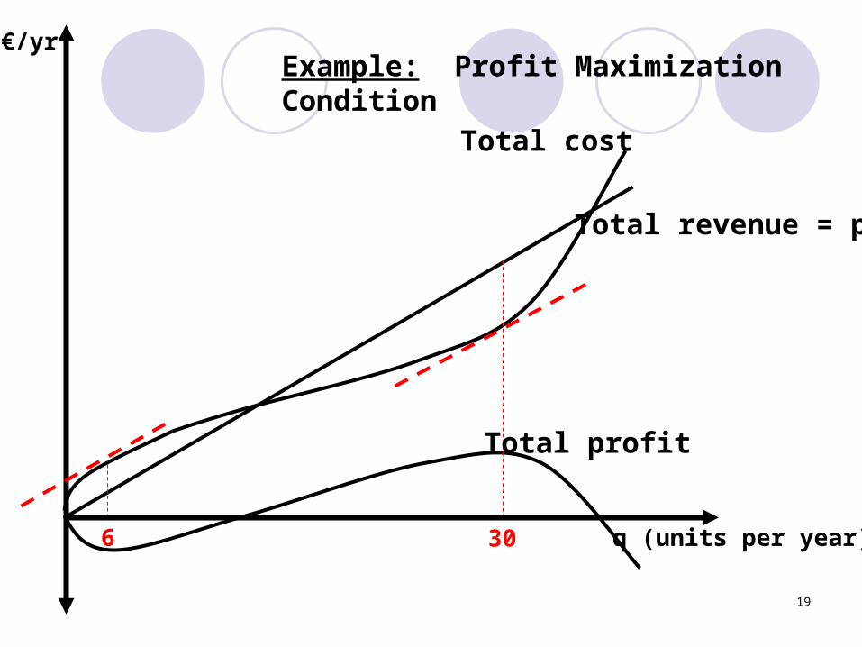
19

€/yr

q (units per year)

Total profit

306

Example: Profit Maximization Condition

Total cost

Total revenue = pq

20

Example: Profit Maximization Condition

q (units per year)

q (units per year)

Total revenue = pq

P, MR15

€/yr

21

Example: Profit Maximization Condition

q (units per year)

q (units per year)

P, MR

MC

Total Cost

€/yr

15

Total revenue = pq

22

Example: Profit Maximization Condition

q (units per year)

q (units per year)

P, MR

MC

Total Cost

6 30

€/yr

15

Total revenue = pq

23

Notes: At profit maximizing point:

P = MC MC is non-decreasing

24

Notes: What is the firm’s demand curve?

The firm can sell as much as it likes at price P, so the firm’s demand curve is a straight line at P

What is the firm’s supply curve? It is defined by the MC curve, but not in

its entirety.

25

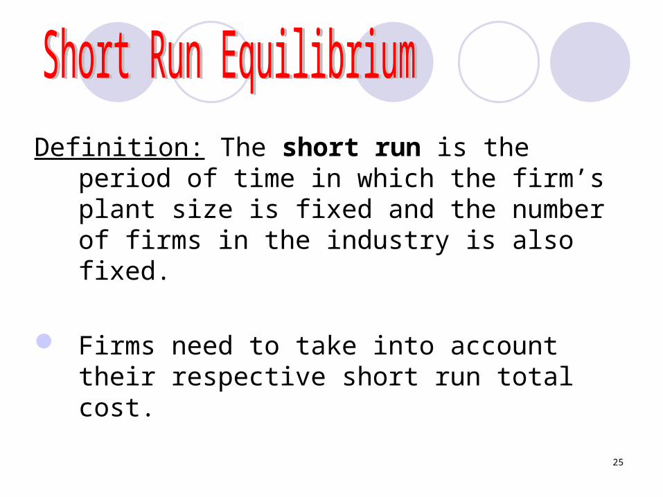
Definition: The short run is the period of time in which the firm’s plant size is fixed and the number of firms in the industry is also fixed.

Firms need to take into account their respective short run total cost.

26

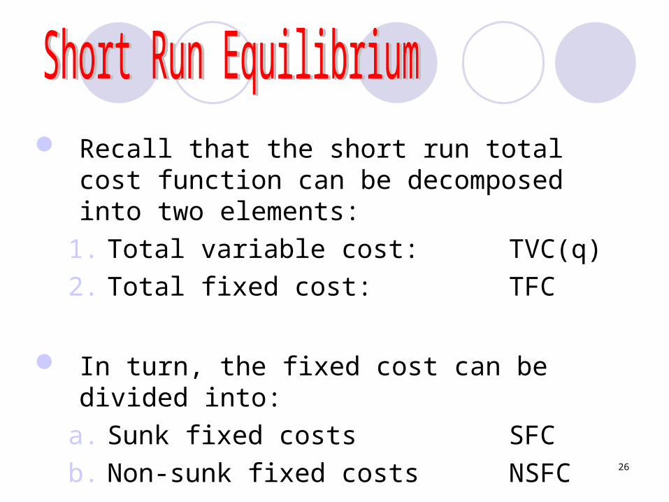
Recall that the short run total cost function can be decomposed into two elements:

1. Total variable cost: TVC(q)2. Total fixed cost: TFC

In turn, the fixed cost can be divided into:a. Sunk fixed costs SFCb. Non-sunk fixed costs NSFC

27

Then: TVC(q) + SFC + NSFC when

q > 0TC(q) =

SFCwhen q = 0

Obviously TFC = SFC + NSFC

28

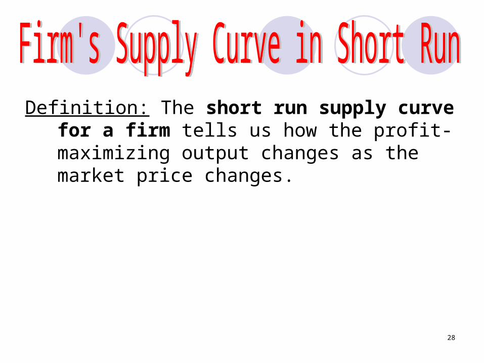
Definition: The short run supply curve for a firm tells us how the profit-maximizing output changes as the market price changes.

29

General Idea: If the firm chooses to produce q > 0, then

condition P = SMC defines short run supply curve of the firm.

The firm produces q > 0 as long as:(q) (0)

If (q) < (0), then the firm shuts down.

30

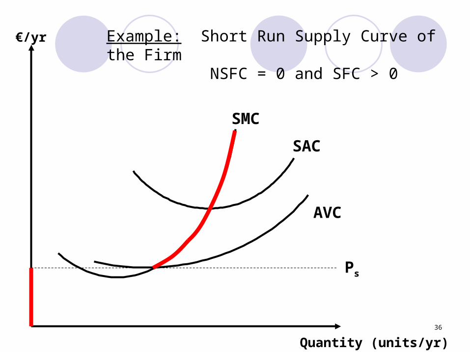
Definition: The shut-down price, Ps, is the price below which the firm would opt to produce zero.

The firm’s short run supply function is defined by:

SMC when P PS

s(P) = 0 when P < PS

31

The value of Ps depends on the structure of the fixed costs. In particular, whether there are sunk costs or not.

Let’s look at two cases:1. All fixed costs are sunk

NSFC = 0 and SFC > 0 ==> (0) = SFC

2. All fixed costs are non-sunkNSFC > 0 and SFC = 0 ==> (0) = 0

32

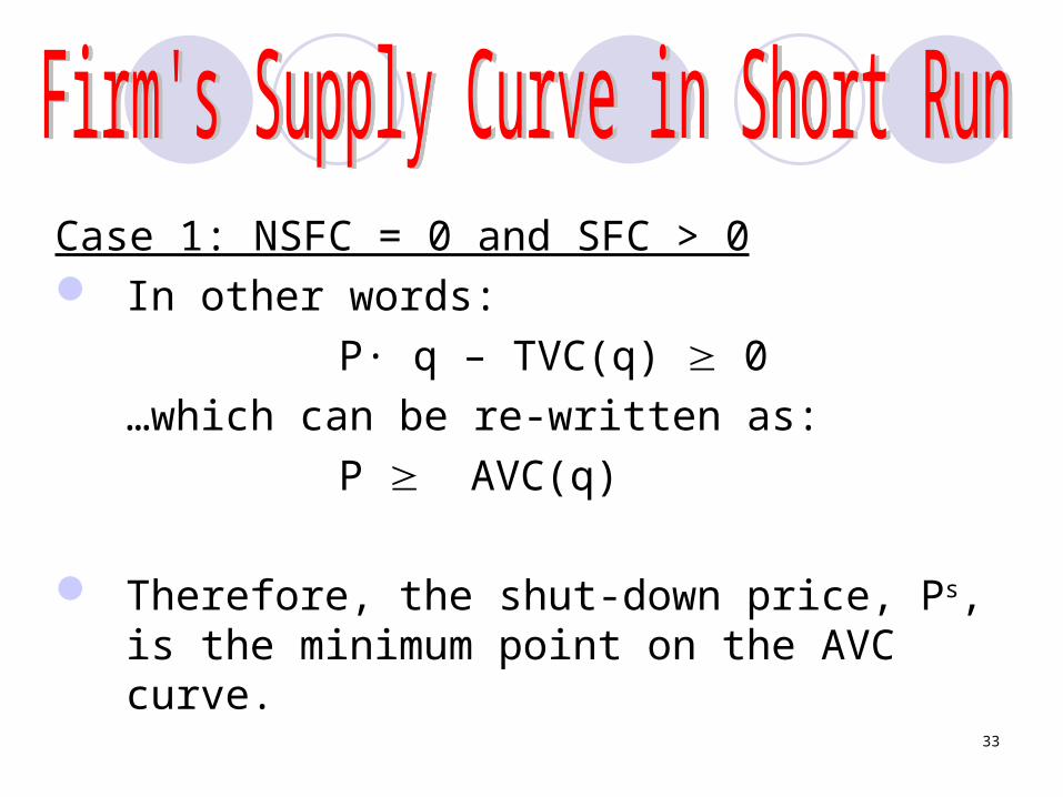
Case 1: NSFC = 0 and SFC > 0 Hence, TFC = SFC (fixed costs are all

sunk) The firm will choose to produce a positive

output only if:

(q) (0) …or…

P· q – TVC(q) – TFC – TFC = – SFC

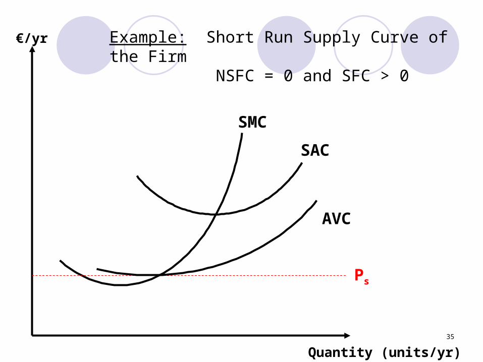
33

Case 1: NSFC = 0 and SFC > 0 In other words:

P· q – TVC(q) 0…which can be re-written as:

P AVC(q)

Therefore, the shut-down price, Ps, is the minimum point on the AVC curve.

34

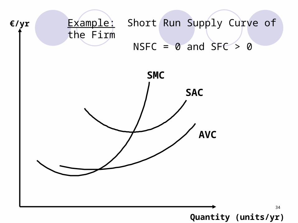
Quantity (units/yr)

€/yr

AVC

SAC

SMC

Example: Short Run Supply Curve of the Firm

NSFC = 0 and SFC > 0

35

Quantity (units/yr)

€/yr

AVC

SAC

SMC

Ps

Example: Short Run Supply Curve of the Firm

NSFC = 0 and SFC > 0

36

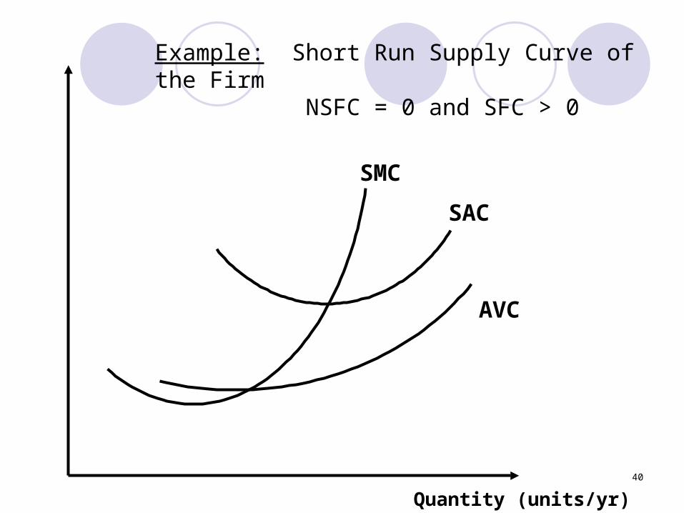
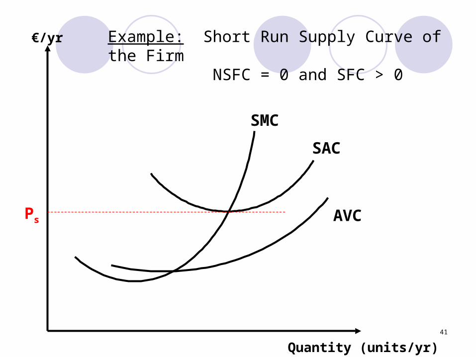
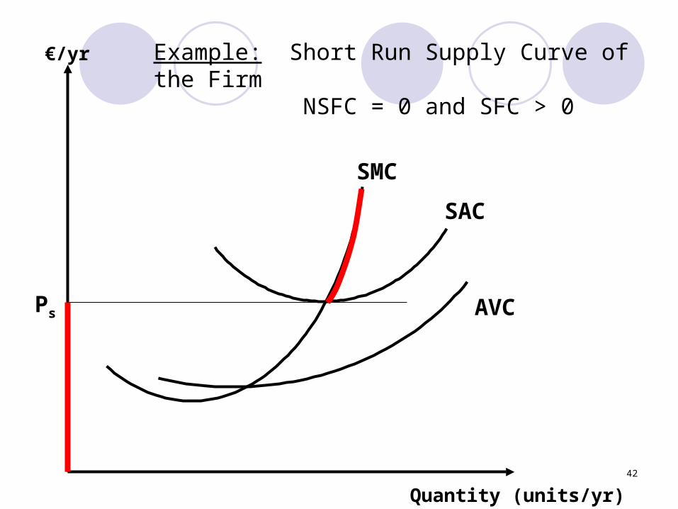
Example: Short Run Supply Curve of the Firm

NSFC = 0 and SFC > 0

Quantity (units/yr)

€/yr

AVC

SAC

SMC

Ps

37

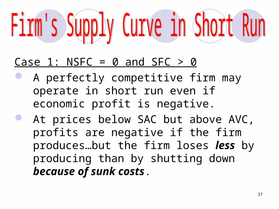
Case 1: NSFC = 0 and SFC > 0 A perfectly competitive firm may operate

in short run even if economic profit is negative.

At prices below SAC but above AVC, profits are negative if the firm produces…but the firm loses less by producing than by shutting down because of sunk costs.

38

Case 2: NSFC > 0 and SFC = 0 The firm will choose to produce a positive

output only if:

(q) (0) …or…

P· q – TVC(q) – TFC 0

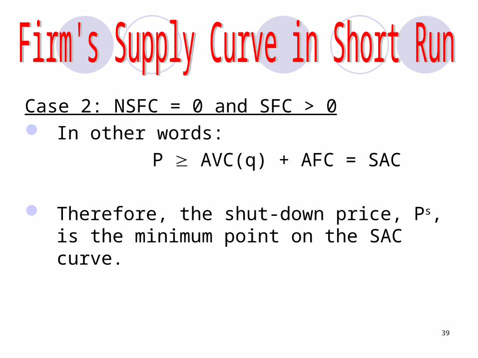
39

Case 2: NSFC = 0 and SFC > 0 In other words:

P AVC(q) + AFC = SAC

Therefore, the shut-down price, Ps, is the minimum point on the SAC curve.

40

AVC

SAC

SMC

Example: Short Run Supply Curve of the Firm

NSFC = 0 and SFC > 0

Quantity (units/yr)

41

Quantity (units/yr)

€/yr

AVC

SAC

SMC

Ps

Example: Short Run Supply Curve of the Firm

NSFC = 0 and SFC > 0

42

AVC

SAC

SMC

Ps

Example: Short Run Supply Curve of the Firm

NSFC = 0 and SFC > 0

Quantity (units/yr)

€/yr

43

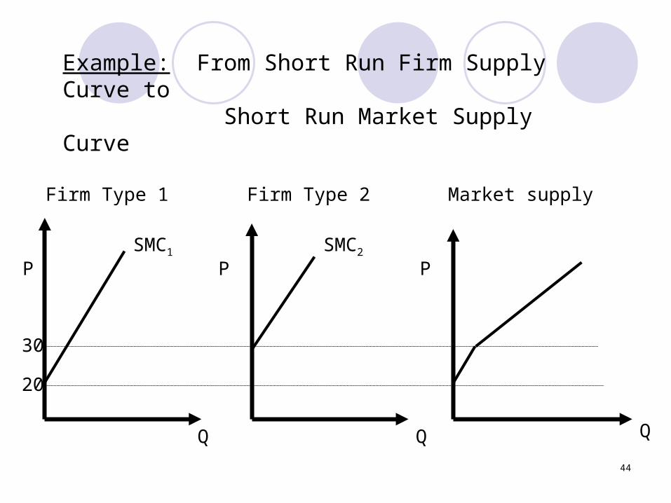
Definition: The market supply at any price is the

sum of the quantities each firm supplies at that price.

The short run market supply curve is the horizontal sum of the individual firm supply curves.

44

Firm Type 1 Firm Type 2 Market supply

30

Q Q Q

P P PSMC1

20

SMC2

Example: From Short Run Firm Supply Curve to Short Run Market Supply Curve

45

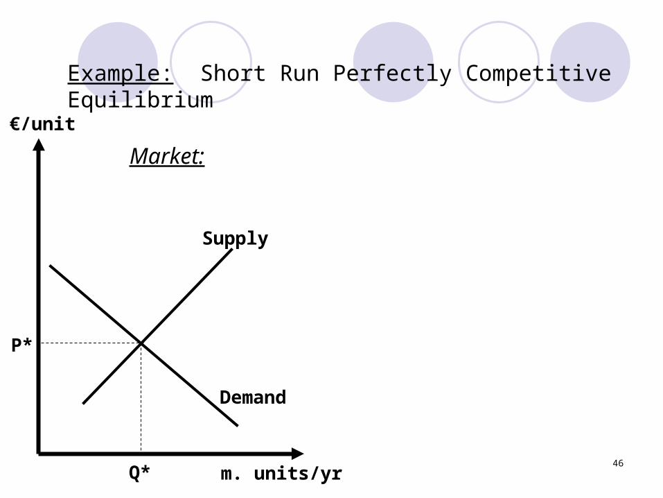
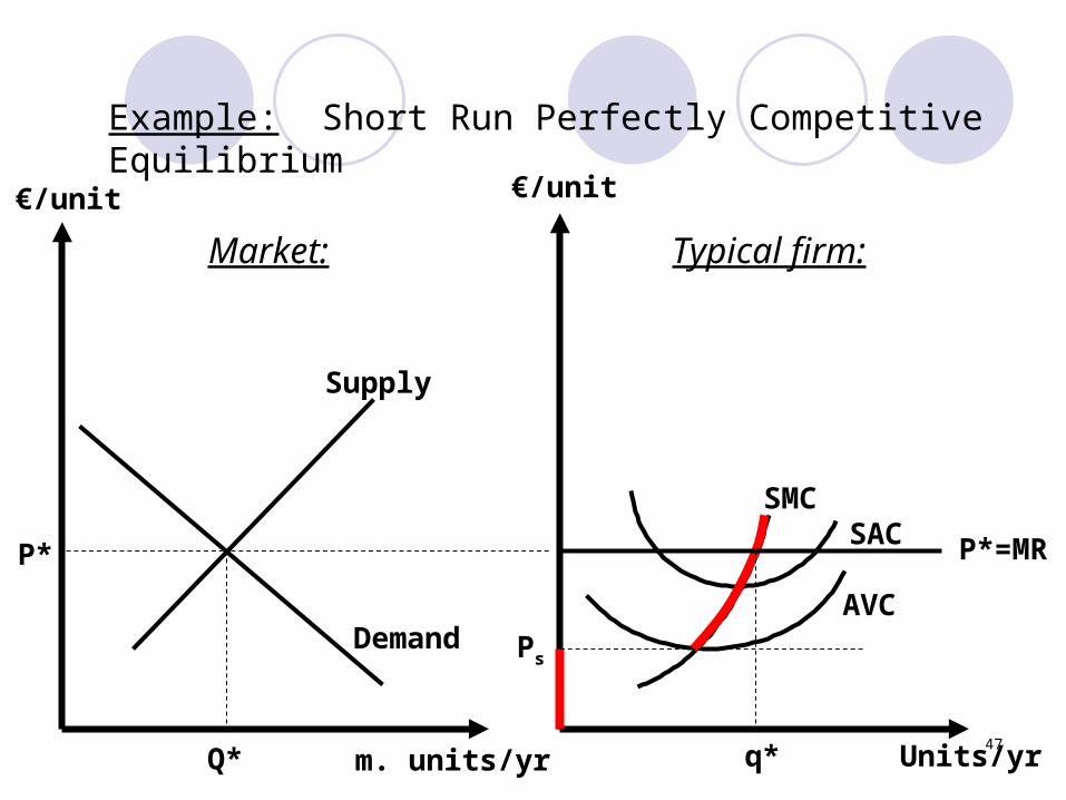
Definition: A short run perfectly competitive equilibrium occurs when the market quantity demanded equals the market quantity supplied:

ni=1 qs(P) = Qd(P)

where qs(P) is determined by the firm's individual profit maximization condition.

46

Market:

Example: Short Run Perfectly Competitive Equilibrium

P*

Demand

Supply

€/unit

Q* m. units/yr

47

Market: Typical firm:

Example: Short Run Perfectly Competitive Equilibrium

SMCSAC

AVCPs

P*

Demand

Supply

€/unit€/unit

Q* q* Units/yrm. units/yr

P*=MR

48

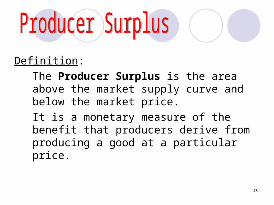
Definition: The Producer Surplus is the area above the market supply curve and below the market price.It is a monetary measure of the benefit that producers derive from producing a good at a particular price.

49

Example: Producer Surplus

Q

P

Market Supply Curve

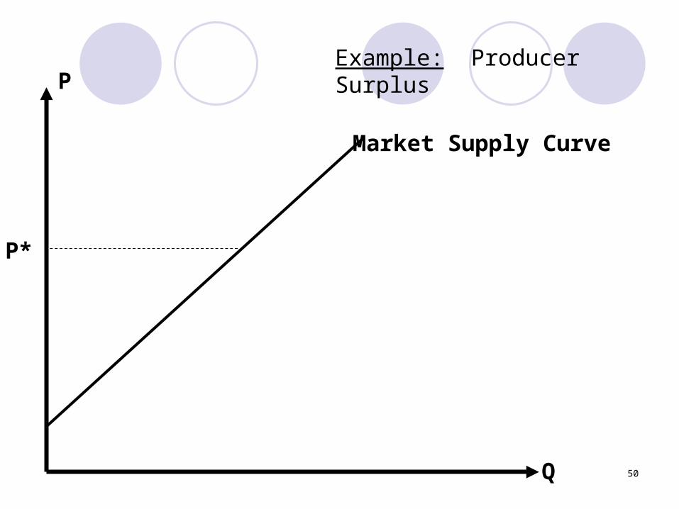
50

Example: Producer Surplus

Q

P

Market Supply Curve

P*

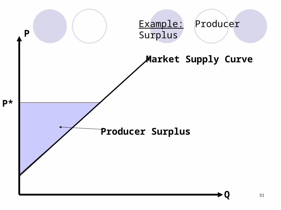
51

Example: Producer Surplus

Q

P

Market Supply Curve

P*

Producer Surplus

52

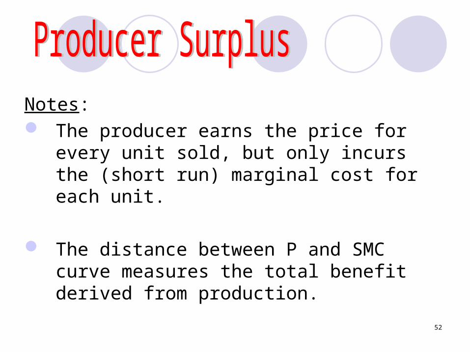
Notes: The producer earns the price for every

unit sold, but only incurs the (short run) marginal cost for each unit.

The distance between P and SMC curve measures the total benefit derived from production.

53

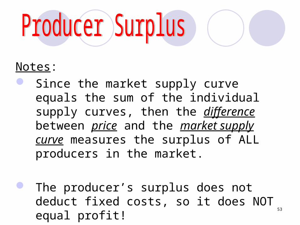
Notes: Since the market supply curve equals the

sum of the individual supply curves, then the difference between price and the market supply curve measures the surplus of ALL producers in the market.

The producer’s surplus does not deduct fixed costs, so it does NOT equal profit!

54

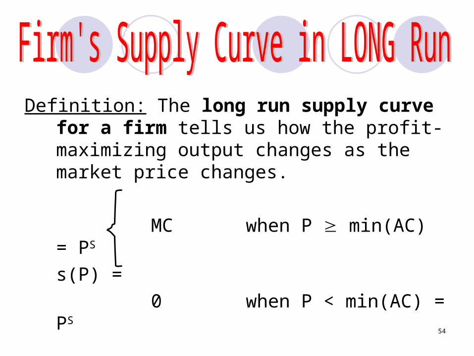
Definition: The long run supply curve for a firm tells us how the profit-maximizing output changes as the market price changes.

MC when P min(AC) = PS

s(P) = 0 when P < min(AC) =

PS

55

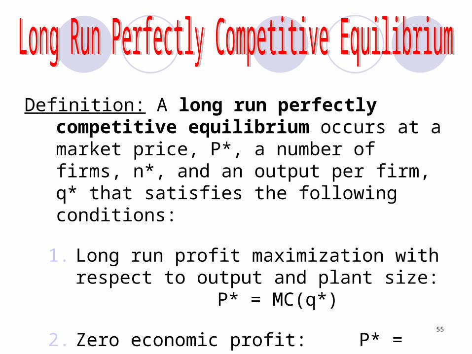
Definition: A long run perfectly competitive equilibrium occurs at a market price, P*, a number of firms, n*, and an output per firm, q* that satisfies the following conditions:

1. Long run profit maximization with respect to output and plant size:

P* = MC(q*)

2. Zero economic profit: P* = AC(q*)

3. Demand equals supply: Qd(P*) = n*q*

56

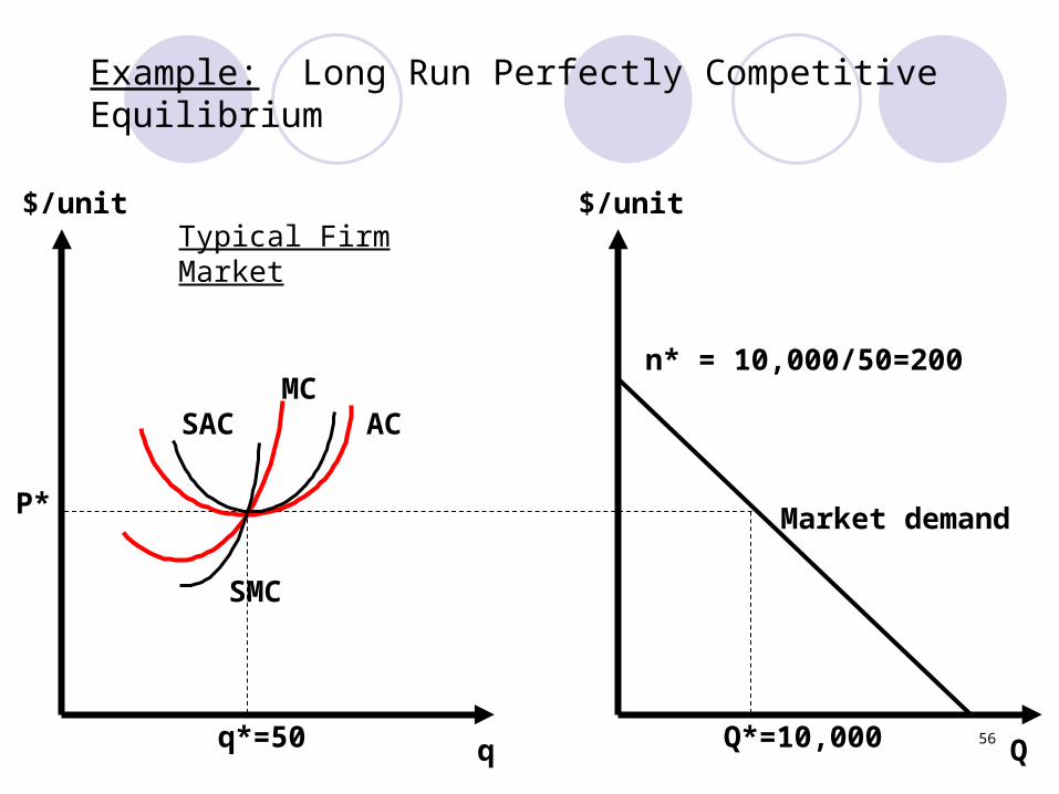
Example: Long Run Perfectly Competitive Equilibrium

Typical Firm Market

ACMC

SAC

SMC

P*

q*=50 q Q

$/unit$/unit

Market demand

Q*=10,000

n* = 10,000/50=200

57

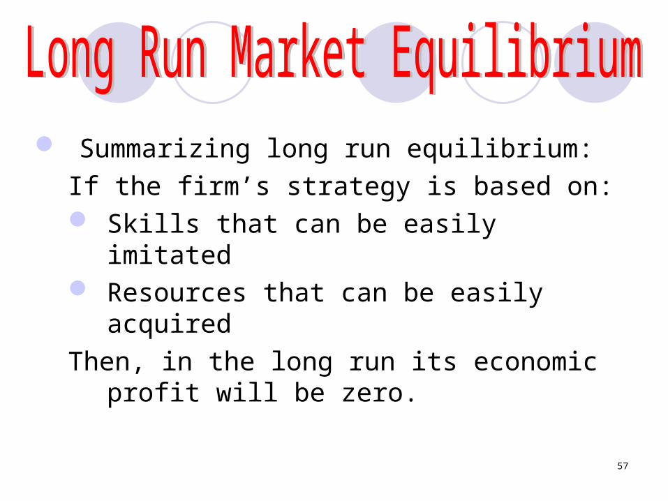
Summarizing long run equilibrium:If the firm’s strategy is based on: Skills that can be easily imitated Resources that can be easily acquiredThen, in the long run its economic profit

will be zero.

58

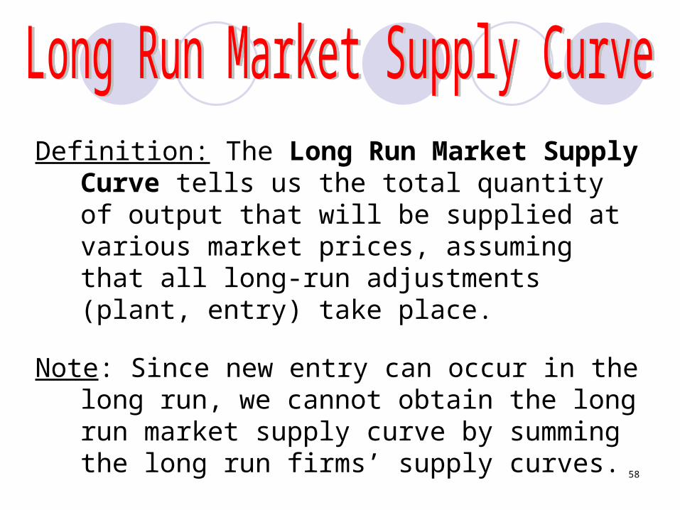
Definition: The Long Run Market Supply Curve tells us the total quantity of output that will be supplied at various market prices, assuming that all long-run adjustments (plant, entry) take place.

Note: Since new entry can occur in the long run, we cannot obtain the long run market supply curve by summing the long run firms’ supply curves.

59

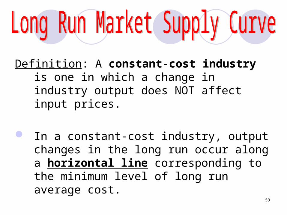
Definition: A constant-cost industry is one in which a change in industry output does NOT affect input prices.

In a constant-cost industry, output changes in the long run occur along a horizontal line corresponding to the minimum level of long run average cost.

60

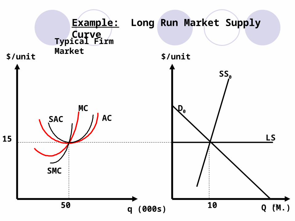
In a constant-cost industry: If P > min(AC), entry would occur,

driving price back to min(AC) If P < min(AC), firms would earn

negative profits and would supply nothing

61

Typical Firm Market

Example: Long Run Market Supply Curve

ACMC

SAC

SMC

15

50 q (000s) Q (M.)

$/unit$/unit

10

SS0

D0

LS

62

Typical Firm Market

Example: Long Run Market Supply Curve

ACMC

SAC

SMC

15

50 52 q (000s) Q (M.)

$/unit$/unit

10

SS0

23

D0

D1

LS

63

Typical Firm Market

Example: Long Run Market Supply Curve

ACMC

SAC

SMC

15

50 52 q (000s) Q (M.)

$/unit$/unit

10 18

SS0

23

D0

D1

SS1

LS

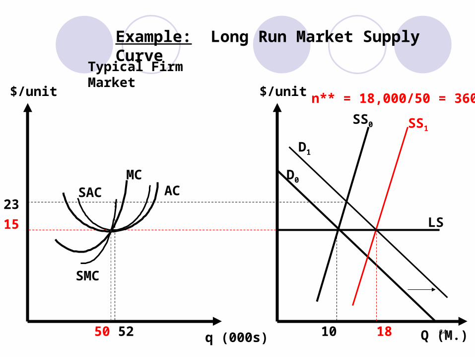
64

Typical Firm Market

Example: Long Run Market Supply Curve

ACMC

SAC

SMC

15

50 52 q (000s) Q (M.)

$/unit$/unit

10 18

n** = 18,000/50 = 360

SS0

23

D0

D1

SS1

LS

65

1. Perfectly Competitive markets have the following characteristics:

a. Homogeneous productsb. Perfect informationc. Atomicity or fragmentation (small

buyers and sellers)d. Equal access to resources

66

2. A price taking firm maximizes profit by producing at an output level at which (rising) marginal cost equals the market price (which is the marginal revenue for a price-taking firm).

3. If all fixed costs are sunk, a perfectly competitive firm will produce positive output in the short run only if market price exceeds AVC.

4. The short run market supply is the horizontal sum of the short run supplies of individual firms.