Lecture 12Statistical Inference (Estimation)

Point and Interval estimationBy

Aziza Munir

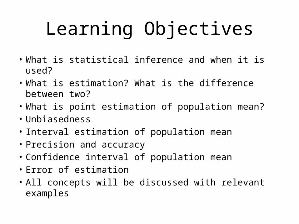
Learning Objectives

• What is statistical inference and when it is used?• What is estimation? What is the difference between

two?• What is point estimation of population mean?• Unbiasedness• Interval estimation of population mean• Precision and accuracy• Confidence interval of population mean• Error of estimation• All concepts will be discussed with relevant examples

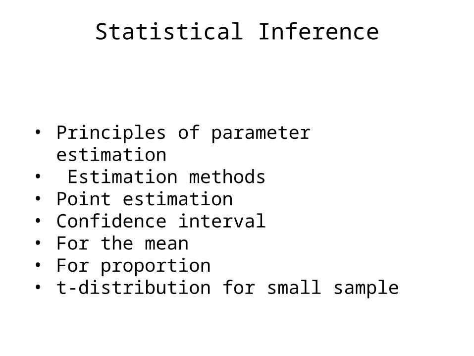
Statistical Inference

• Principles of parameter estimation• Estimation methods• Point estimation• Confidence interval• For the mean• For proportion• t-distribution for small sample

Definition

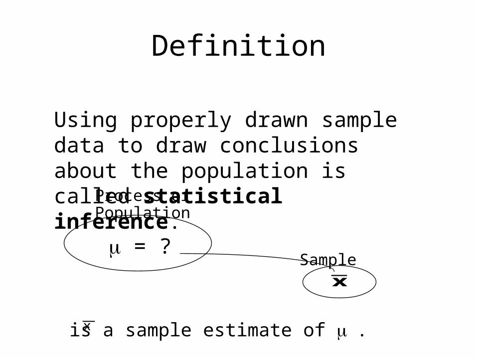
Using properly drawn sample data to draw conclusions about the population is called statistical inference.

Process or Population

m = ?

xSample

is a sample estimate of m .x

Statistical Inference

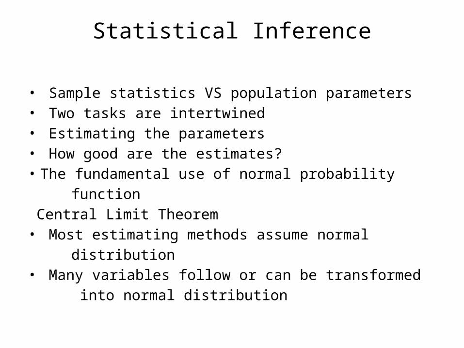
• Sample statistics VS population parameters• Two tasks are intertwined• Estimating the parameters• How good are the estimates?• The fundamental use of normal probability function Central Limit Theorem• Most estimating methods assume normal distribution• Many variables follow or can be transformed into normal distribution

Definitions

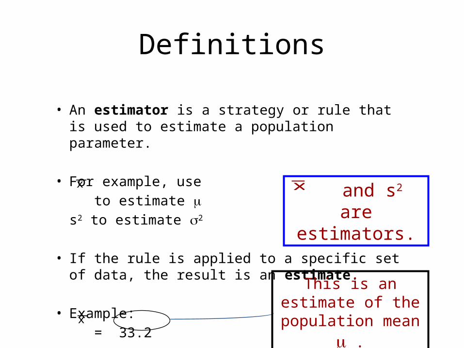
• An estimator is a strategy or rule that is used to estimate a population parameter.

• For example, use to estimate m s2 to estimate s2

• If the rule is applied to a specific set of data, the result is an estimate.

• Example: = 33.2

x and s2 are estimators.

x

x

This is an estimate of the population mean

m .

Statistical Inference

• Statistical inference permits the estimation of statistical measures (means, proportions, etc.) with a known degree of confidence.

• This ability to assess the quality (confidence) of estimates is one of the significant benefits statistics brings to decision making and problem solving.

Randomly Selected Samples

• If samples are selected randomly, the uncertainty of the inference is measurable.

• The ability to measure the confidence associated with a statistical inference is the value received for drawing random samples.

• If samples are not selected randomly, there will be no known relationship between the sample results and the population.

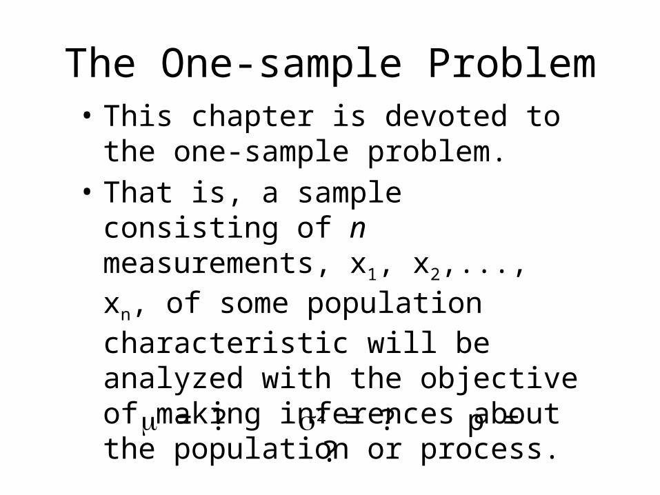
The One-sample Problem• This chapter is devoted to the one-

sample problem.• That is, a sample consisting of n

measurements, x1, x2,..., xn, of some population characteristic will be analyzed with the objective of making inferences about the population or process.

m = ? s2 = ? p = ?

Principles of Parameter Estimation

Unbiased• The expected value of the estimate is equal to population parameterConsistent As n (sample size) approaches N (population size), estimator converges to the population parameter Efficient• With the smallest variance.• Sufficient• Contains all information about the parameter through a sample of size n

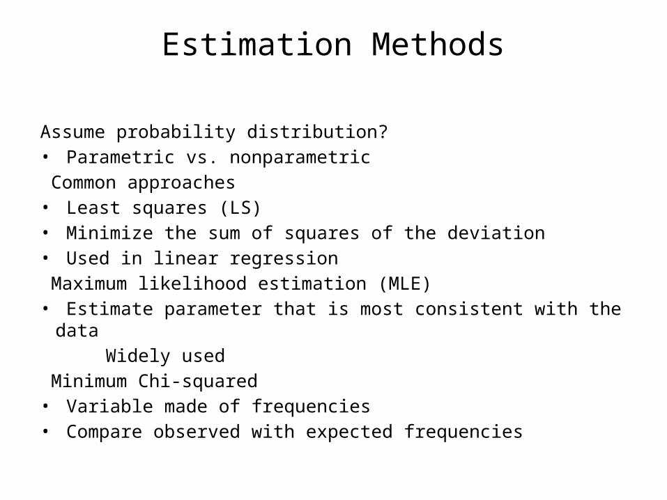
Estimation Methods

Assume probability distribution?• Parametric vs. nonparametric Common approaches• Least squares (LS)• Minimize the sum of squares of the deviation• Used in linear regression Maximum likelihood estimation (MLE)• Estimate parameter that is most consistent with the data Widely used Minimum Chi-squared• Variable made of frequencies• Compare observed with expected frequencies

Judgment Estimates

• Many estimates are subjective, that is, a person with experience in the field is utilized to estimate an unknown population value.

• The problem with judgment estimates is that their degree of accuracy or inaccuracy cannot be determined.

• Even if experts exist, statistics offers estimates with known reliability.

Point Estimation of the Population Mean

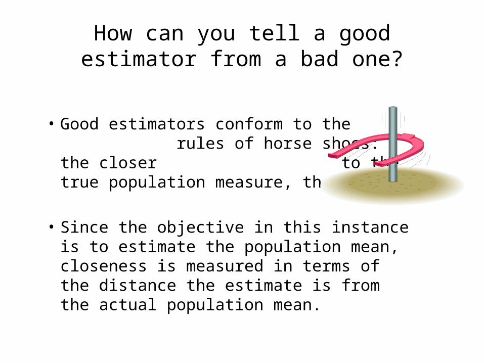
How can you tell a good estimator from a bad one?

• Good estimators conform to the rules of horse shoes: the closer to the true population measure, the better.

• Since the objective in this instance is to estimate the population mean, closeness is measured in terms of the distance the estimate is from the actual population mean.

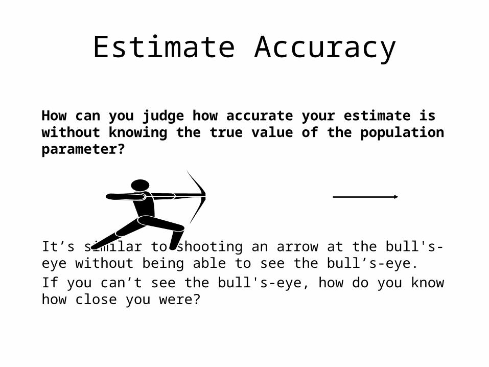
Estimate Accuracy

How can you judge how accurate your estimate is without knowing the true value of the population parameter?

It’s similar to shooting an arrow at the bull's-eye without being able to see the bull’s-eye. If you can’t see the bull's-eye, how do you know how close you were?

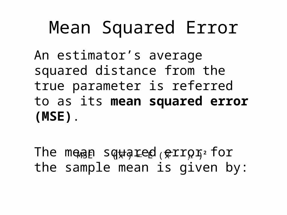
Mean Squared ErrorAn estimator’s average squared distance from the true parameter is referred to as its mean squared error (MSE).

The mean squared error for the sample mean is given by:

MSE(x) E(x ) 2

Finding an Estimator

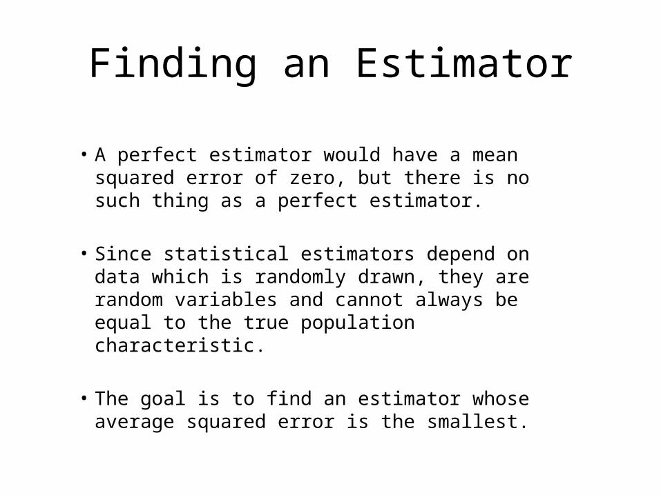
• A perfect estimator would have a mean squared error of zero, but there is no such thing as a perfect estimator.

• Since statistical estimators depend on data which is randomly drawn, they are random variables and cannot always be equal to the true population characteristic.

• The goal is to find an estimator whose average squared error is the smallest.

Restricting Estimators

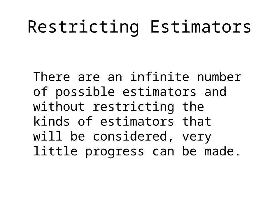
There are an infinite number of possible estimators and without restricting the kinds of estimators that will be considered, very little progress can be made.

Unbiasedness

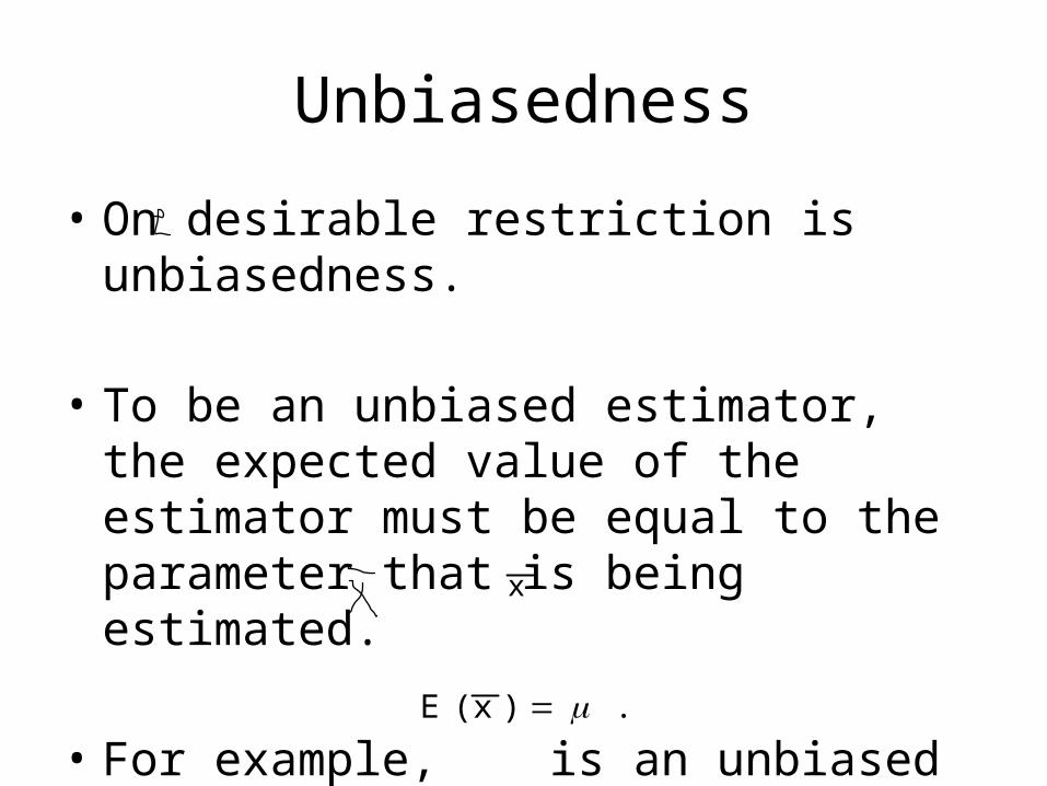
• On desirable restriction is unbiasedness.

• To be an unbiased estimator, the expected value of the estimator must be equal to the parameter that is being estimated.

• For example, is an unbiased estimator of the population mean since

x

E(x) .

Unbiased Estimators

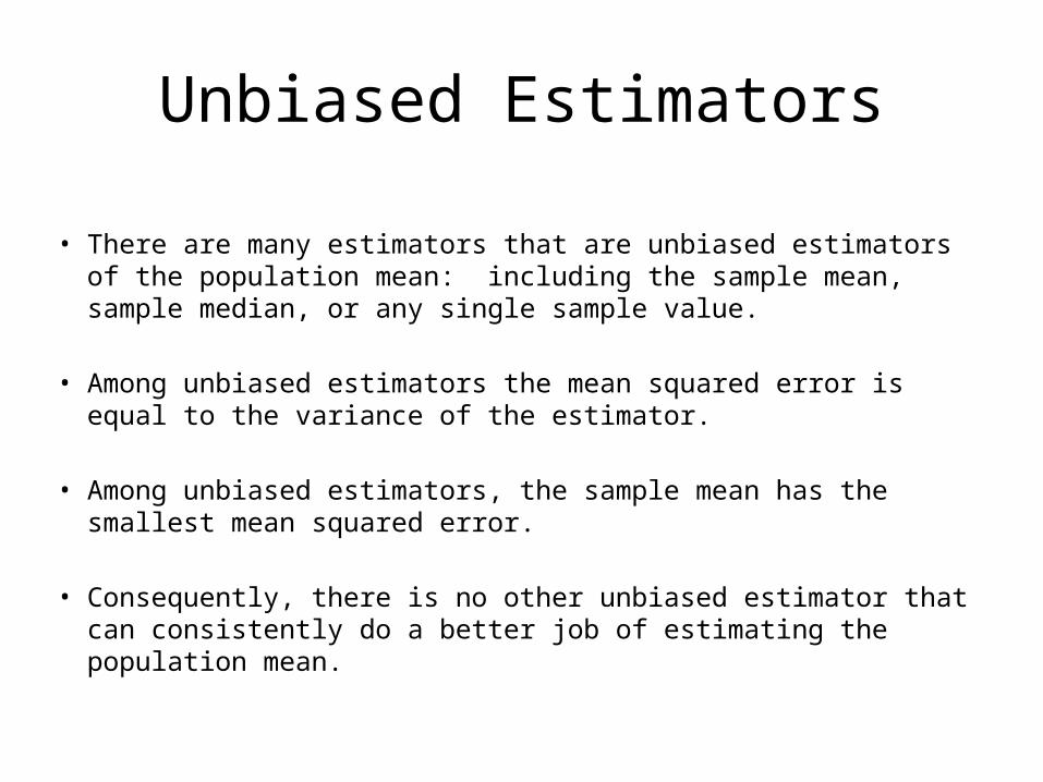
• There are many estimators that are unbiased estimators of the population mean: including the sample mean, sample median, or any single sample value.

• Among unbiased estimators the mean squared error is equal to the variance of the estimator.

• Among unbiased estimators, the sample mean has the smallest mean squared error.

• Consequently, there is no other unbiased estimator that can consistently do a better job of estimating the population mean.

Interval Estimation of the Population Mean

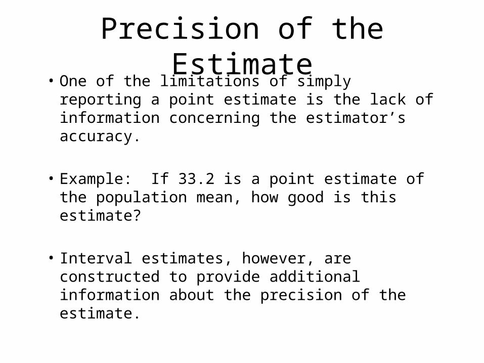
Precision of the Estimate• One of the limitations of simply reporting a

point estimate is the lack of information concerning the estimator’s accuracy.

• Example: If 33.2 is a point estimate of the population mean, how good is this estimate?

• Interval estimates, however, are constructed to provide additional information about the precision of the estimate.

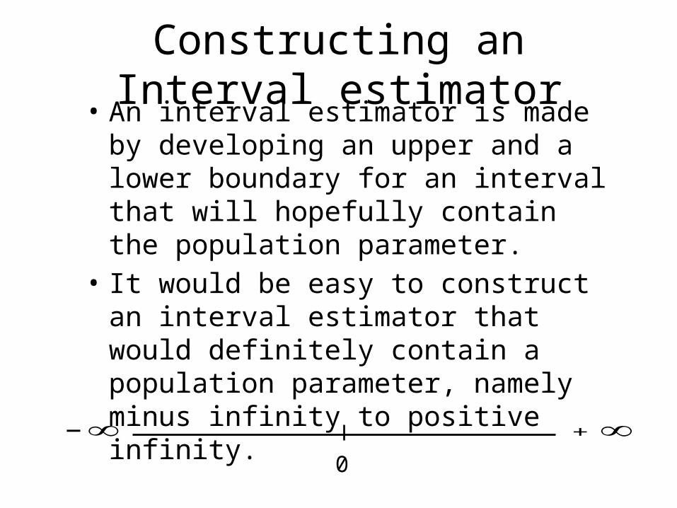
Constructing an Interval estimator• An interval estimator is made by

developing an upper and a lower boundary for an interval that will hopefully contain the population parameter.

• It would be easy to construct an interval estimator that would definitely contain a population parameter, namely minus infinity to positive infinity.

0

- +

Constructing an Interval estimator

• However, this particular interval estimator would not contain any useful information about the location of the population parameter.

• In interval estimation, the smaller the interval for a given amount of confidence, the better.

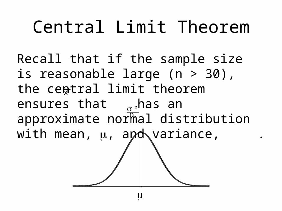
Central Limit Theorem

Recall that if the sample size is reasonable large (n > 30), the central limit theorem ensures that has an approximate normal distribution with mean, m, and variance, .

x

2

n

m

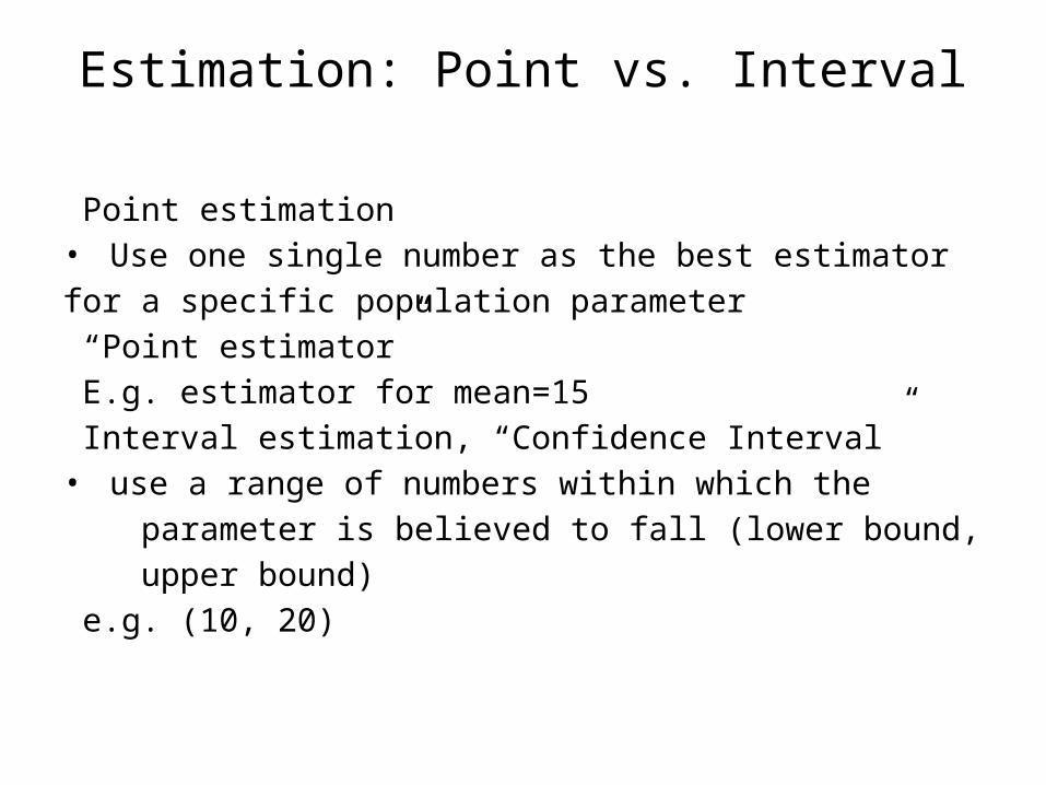
Estimation: Point vs. Interval

Point estimation• Use one single number as the best estimatorfor a specific population parameter “Point estimator” E.g. estimator for mean=15 Interval estimation, “Confidence Interval”• use a range of numbers within which the parameter is believed to fall (lower bound, upper bound) e.g. (10, 20)

Example 1

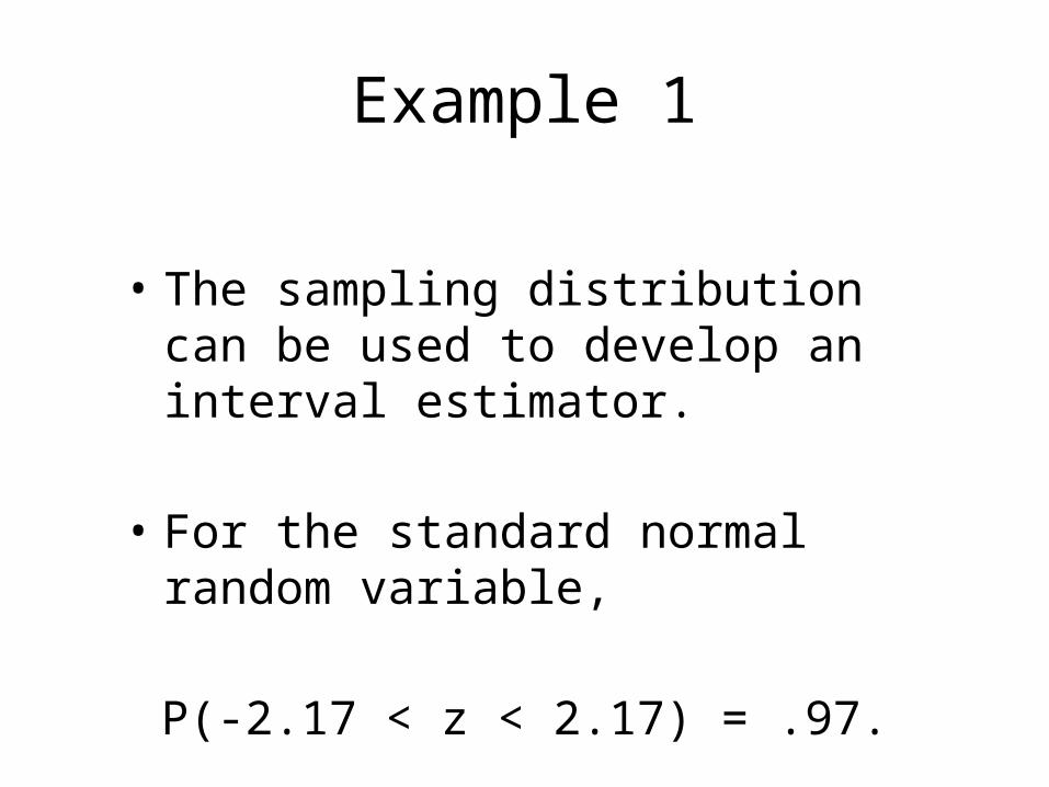
• The sampling distribution can be used to develop an interval estimator.

• For the standard normal random variable,

P(-2.17 < z < 2.17) = .97.

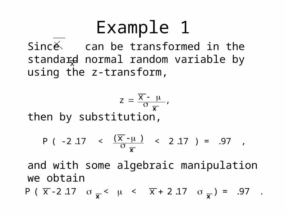
Example 1Since can be transformed in the standard normal random variable by using the z-transform,

then by substitution,

and with some algebraic manipulation we obtain

x

z x

x,

P( -2.17 < (x- ) < 2.17) = .97

x ,

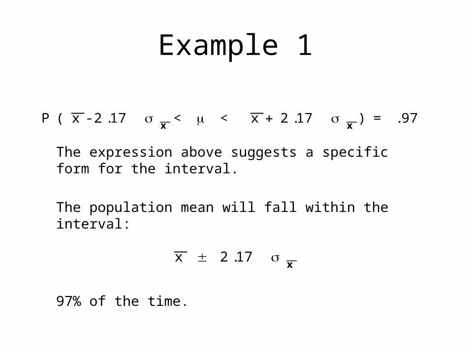
P( x-2.17 < < x 2.17 ) = .97 . x x

Example 1

The expression above suggests a specific form for the interval.

The population mean will fall within the interval:

97% of the time.

x 2.17 x

P( x-2.17 < < x 2.17 ) = .97 x x

Example 1

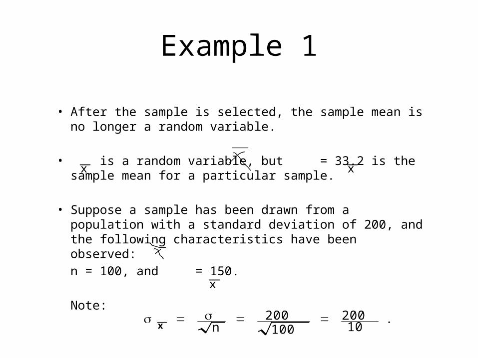
• After the sample is selected, the sample mean is no longer a random variable.

• is a random variable, but = 33.2 is the sample mean for a particular sample.

• Suppose a sample has been drawn from a population with a standard deviation of 200, and the following characteristics have been observed:

n = 100, and = 150.

Note:

x

x .

n200100

20010

xx

Example 1

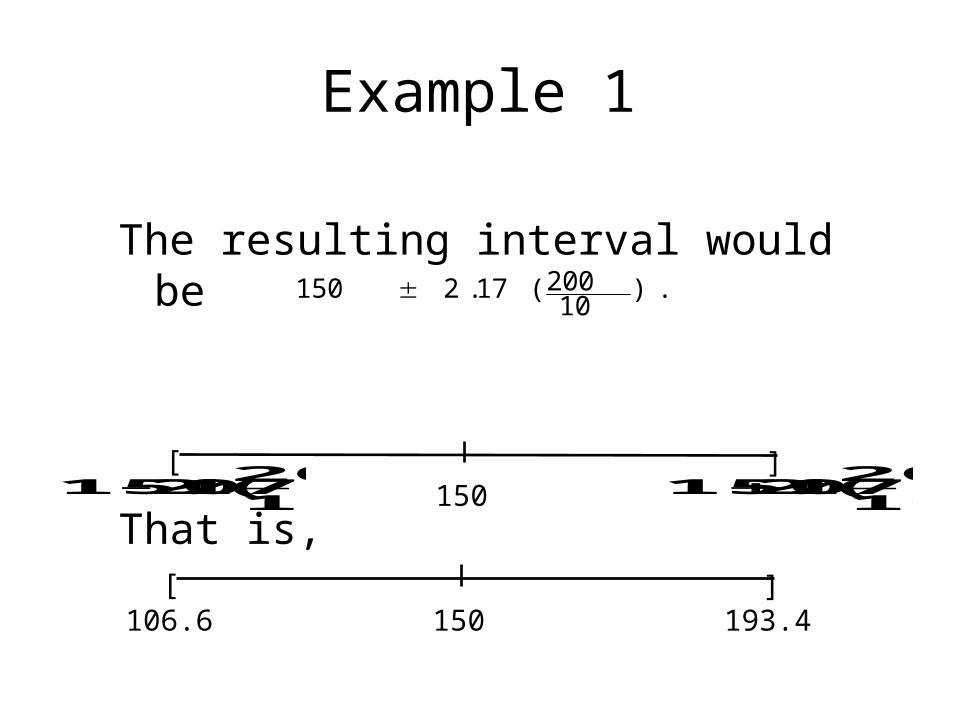
The resulting interval would be

That is,

150 2.17(20010

) .

150 2.17(200

10)150 2.17(

200

10)

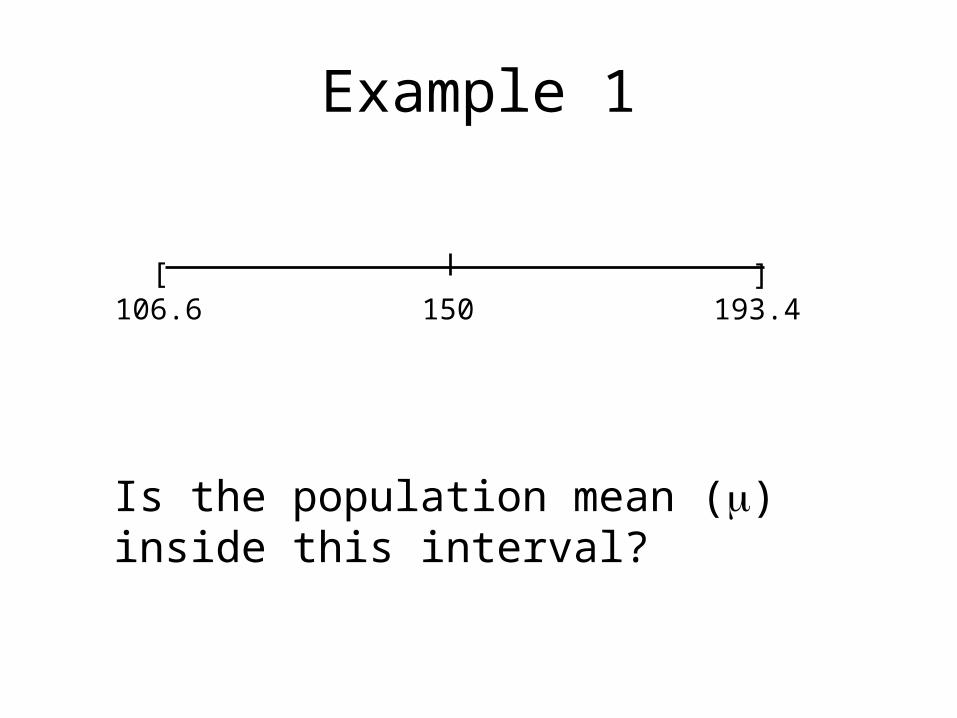
[ ]150

[ ]150106.6 193.4

Example 1

Is the population mean (m) inside this interval?

[ ]150106.6 193.4

Example 1

Even though the interval is calculated using a technique that captures the population mean 97% of the time, it would not be appropriate, from a relative frequency point of view, to state that

P(106.6 < m < 193.4) = .97

since the population mean is an unknown but constant quantity.

Example 1

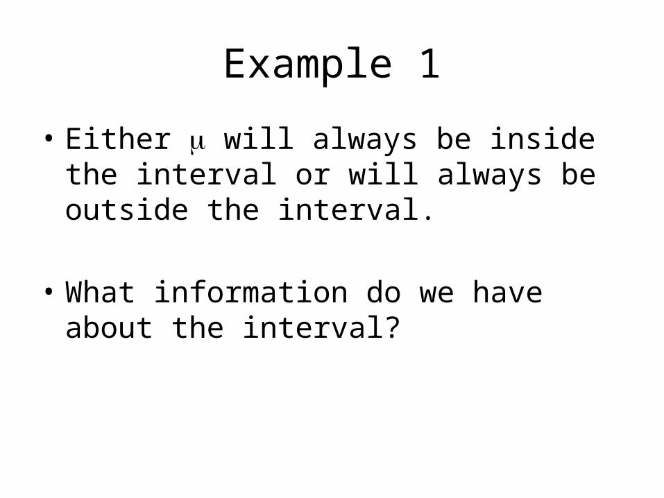
• Either m will always be inside the interval or will always be outside the interval.

• What information do we have about the interval?

Example 1

• Since it was constructed from a technique that will include the true population mean in the interval .97 of the time, we are 97% confident in the technique.

• Confidence is one way of expressing a subjective probability.

• Hence, the term confidence interval is used to describe the method of construction rather than a particular interval.

Example 1

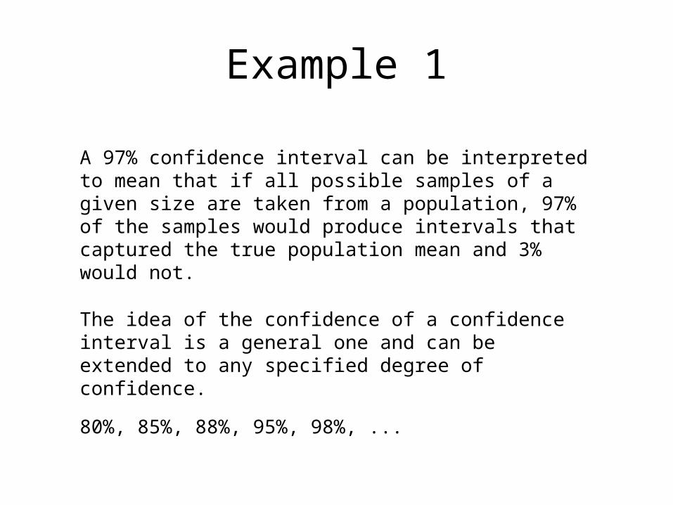
A 97% confidence interval can be interpreted to mean that if all possible samples of a given size are taken from a population, 97% of the samples would produce intervals that captured the true population mean and 3% would not.

The idea of the confidence of a confidence interval is a general one and can be extended to any specified degree of confidence.

80%, 85%, 88%, 95%, 98%, ...

Confidence Interval for the Population Mean

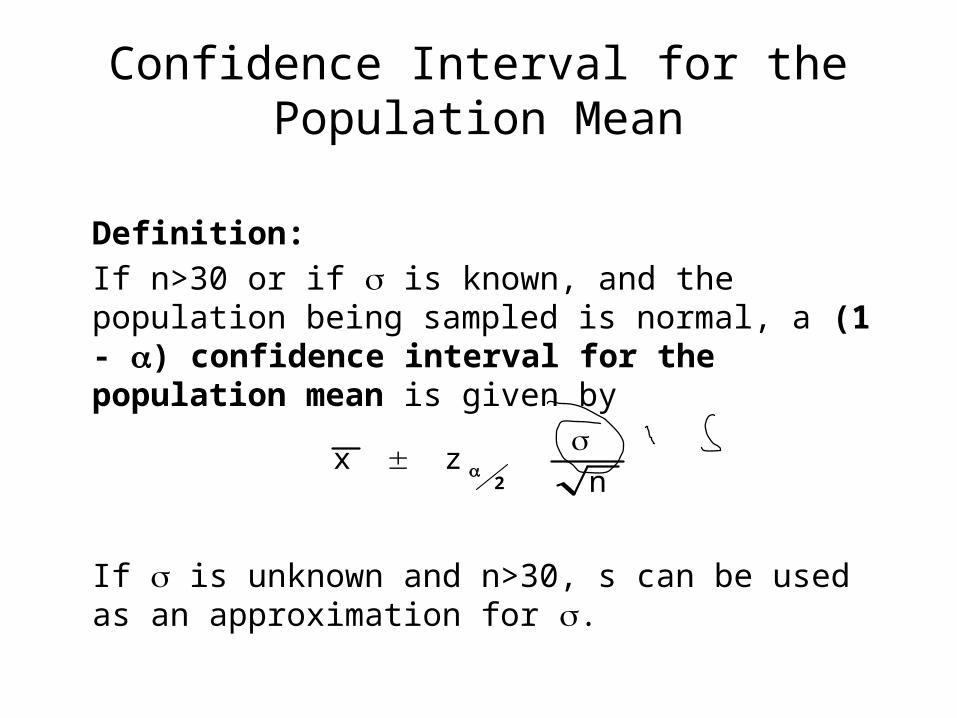
Definition:If n>30 or if s is known, and the population being sampled is normal, a (1 - a) confidence interval for the population mean is given by

If s is unknown and n>30, s can be used as an approximation for s.

x zn

2

Confidence Interval for the Population Mean

The expression, ,

creates the interval shown below.

The term represents thez-value required to obtain an area of 1 - a centered under the standard normal curve.

x zn

2

x zn2

x zn2

[ ]

x

z2

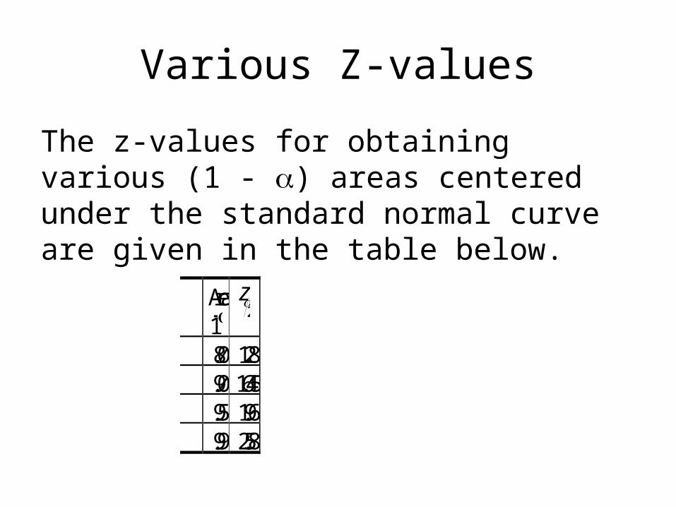
Various Z-values

The z-values for obtaining various (1 - a) areas centered under the standard normal curve are given in the table below.

Area1z2

.801.28

.901.645

.951.96

.992.58

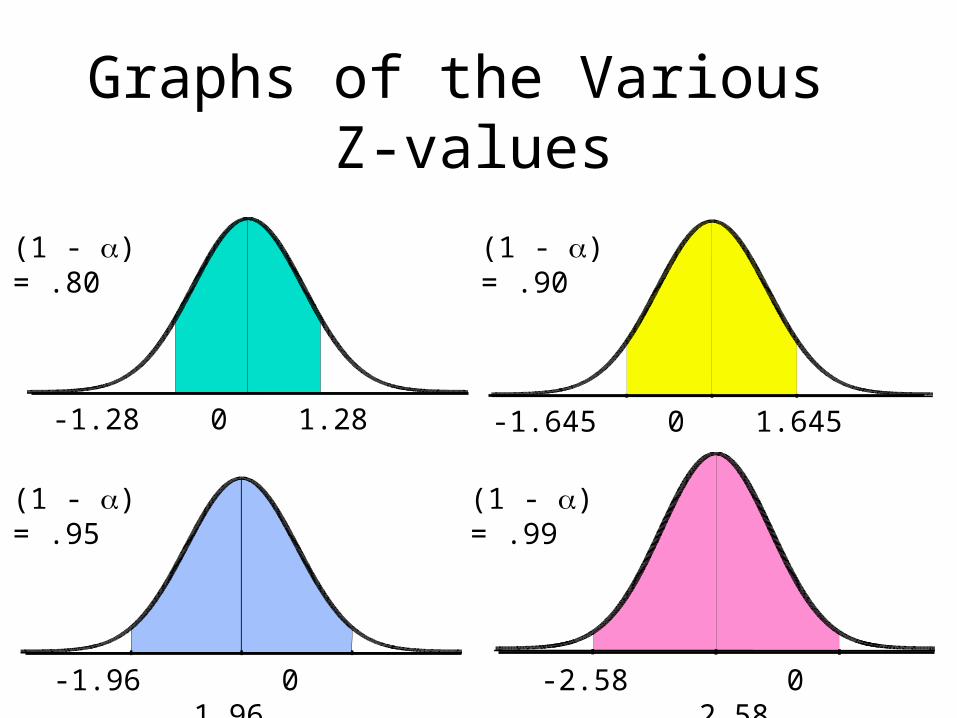
Graphs of the Various Z-values

-1.28 0 1.28 -1.645 0 1.645

-1.96 0 1.96 -2.58 0 2.58

(1 - a) = .80 (1 - a) = .90

(1 - a) = .95 (1 - a) = .99

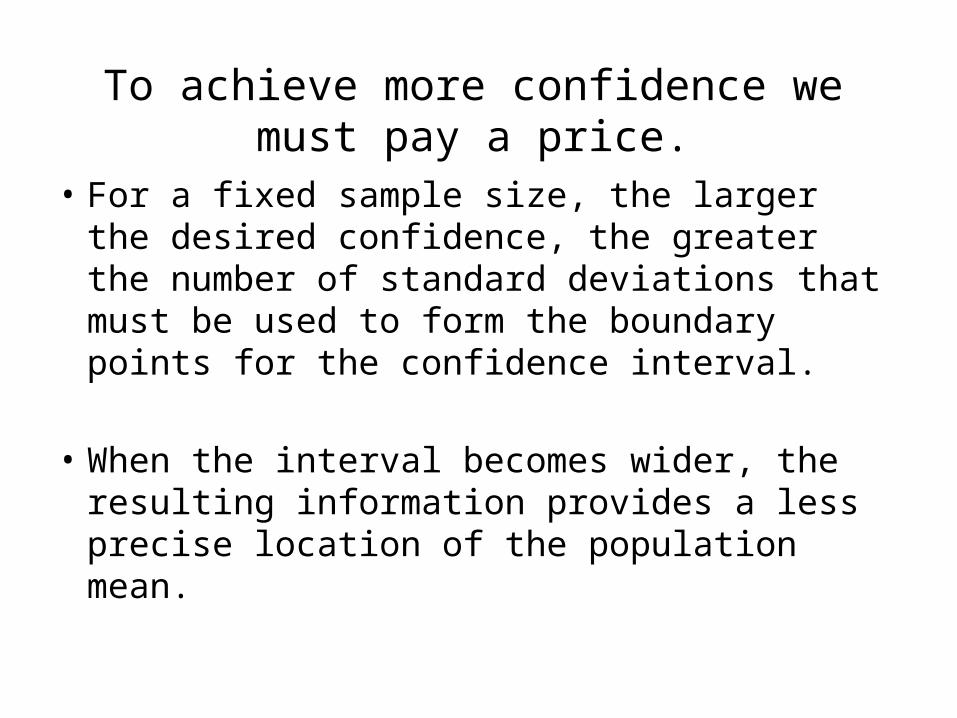
To achieve more confidence we must pay a price.

• For a fixed sample size, the larger the desired confidence, the greater the number of standard deviations that must be used to form the boundary points for the confidence interval.

• When the interval becomes wider, the resulting information provides a less precise location of the population mean.

Error of Estimation

We can also think about the confidence interval as a means of describing the quality of a point estimate.

x zn

2

point estimate maximum error of estimation with a specific level of confidence (1 - a)

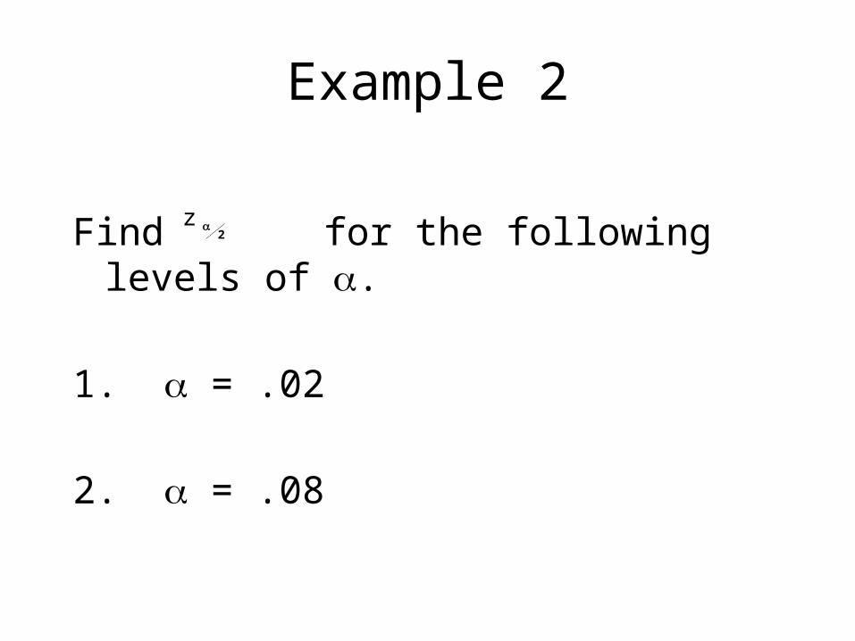
Example 2

Find for the following levels of a.

1. a = .02

2. a = .08

z2

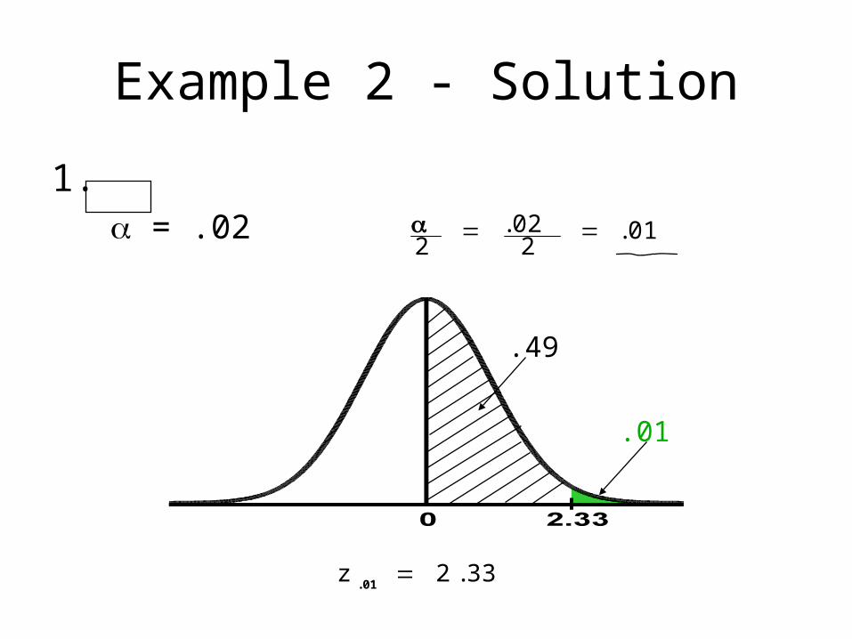
Example 2 - Solution

1. a = .02

2.022

.01

z 2.33.01

.49

.01

Example 2 - Solution

2.a = .08

2.082

.04

z 1.75.04

.46

.04

Example 3

Find for the following confidencelevels:

1. 96%

2. 88%

z2

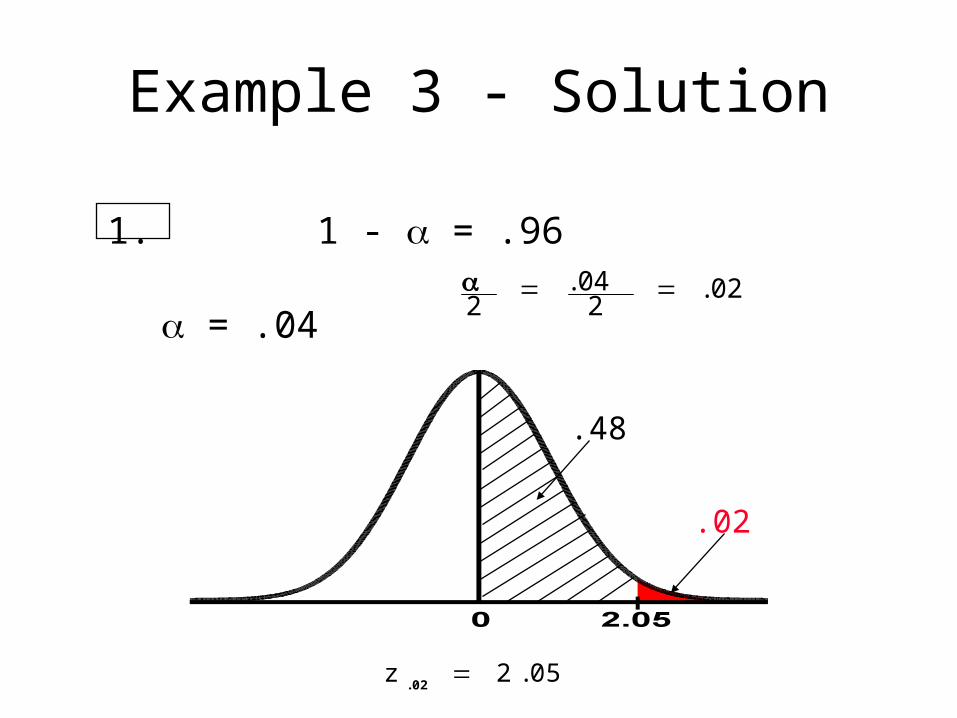
Example 3 - Solution

a = .042

.042

.02

z 2.05.02

1 - a = .961.

.48

.02

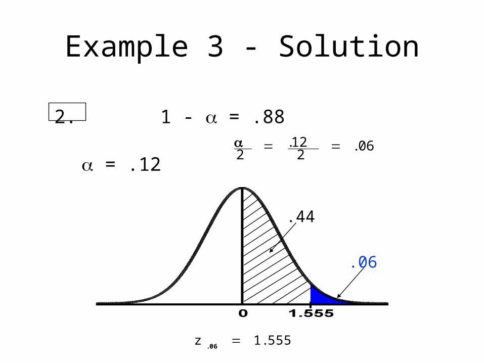
Example 3 - Solution

a = .122

.122

.06

z 1.555.06

1 - a = .882.

.44

.06

Example 4

A paint manufacturer is developing a new type of paint.

Thirty panels were exposed to various corrosive conditions to measure the protective ability of the paint.

The mean life for the samples was 168 hours before corrosive failure.

Example 4

The life of paint samples is assumed to be normally distributed with population standard deviation of 30 hours.

Find the 95% confidence interval for the mean life of the paint.

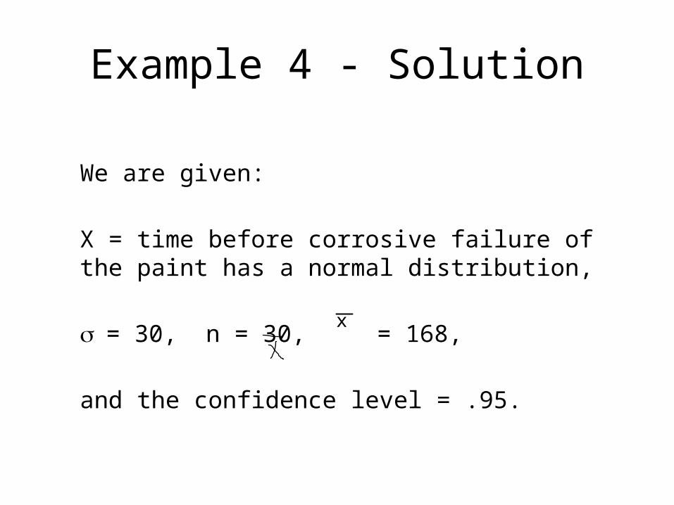
Example 4 - Solution

We are given:

X = time before corrosive failure of the paint has a normal distribution,

s = 30, n = 30, = 168,

and the confidence level = .95.

x

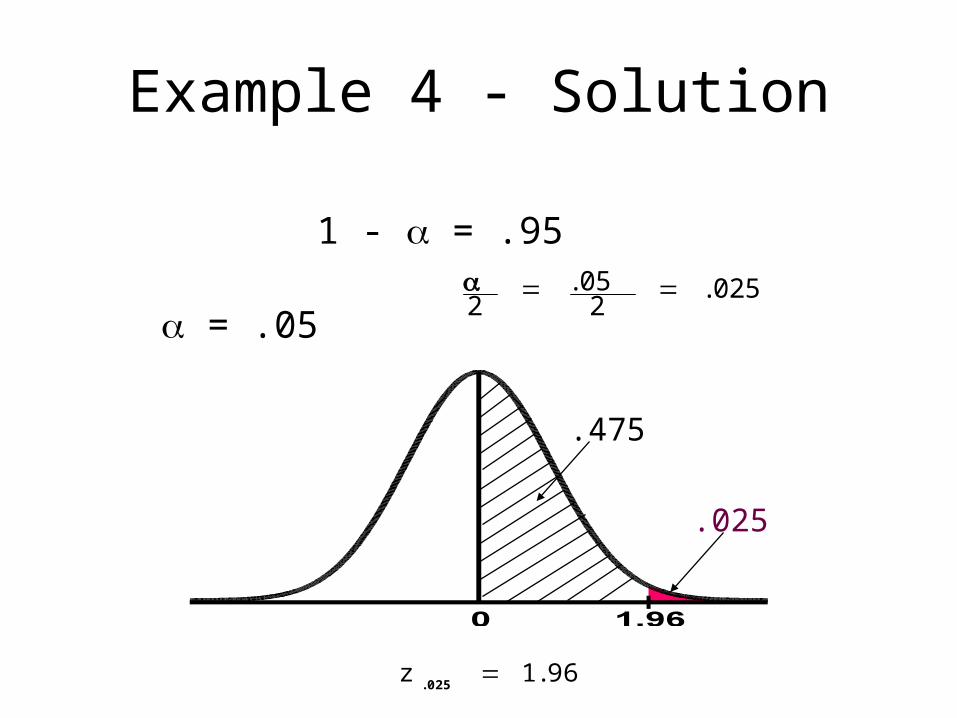
Example 4 - Solution

a = .052

.052

.025

z 1.96.025

1 - a = .95

.475

.025

Conclusion

• Statistical inference• Point and interval estimates• Role of confidence interval and central limit

theorem• Errors of estimation