Lecture 1: Asset pricing and the equity premium puzzlepeople.bu.edu/sgilchri/teaching/EC 745 Fall...
28
Lecture 1: Asset pricing and the equity premium puzzle Simon Gilchrist Boston Univerity and NBER EC 745 Fall, 2013
-
Upload
duongtuyen -
Category
Documents
-
view
214 -
download
0
Transcript of Lecture 1: Asset pricing and the equity premium puzzlepeople.bu.edu/sgilchri/teaching/EC 745 Fall...

Lecture 1: Asset pricing and the equity premiumpuzzle
Simon GilchristBoston Univerity and NBER
EC 745Fall, 2013
Overview
Some basic facts.
Study the asset pricing implications of household portfoliochoice.
Consider the quantitative implications of a second-orderapproximation to asset return equations.
Reference: Mehra and Prescott (JME, 1984)
Some Facts
Stock returns:Average real return on SP500 is 8% per year
Standard error is large since σ(E(R)) = σ(R)√T
)
Stock returns are very volatilie: σ(R) = 17% per year.Stock returns show very little serial correlation (ρ = 0.08quarterly data, -0.04 annual data).
Bond returns:The average risk free rate is 1% per year (US Tbill - Inflation)The risk free rate is not very volatile: σ(R) = 2% per year but ispersistent (ρ = 0.6 in annual data) leading to medium-runvariation.
These imply that the equity premium is large – 7% per year onan annual basis.

S&P 500
0500
1000
1500
sp500
1960q1 1970q1 1980q1 1990q1 2000q1 2010q1date

S&P 500 and value-weighted market return
-150
-100
-500
50100
1960q1 1970q1 1980q1 1990q1 2000q1 2010q1date
ret_sp500 vwxlretd

Recent data (1970-2012)
SP500 Return: Mean = 5.96, Std.Dev = 25.4
Value weighted excess return: mean = 1.56, Std. Dev = 37.54

Return predictability
Cambpell and Shiller (and many others) consider the followingregression:
Ret,t+k = α+ βDt
Pt+ εt
where Ret,t+k is the realized cumulative return over k periods.
k 1y 2y 3y 4y 1y 2y 3y 4yβ 3.83 7.42 11.57 15.81 3.39 6.44 9.99 13.54tstat 2.47 3.13 4.04 4.35 2.18 2.74 3.58 3.83R2 0.07 0.11 0.18 0.20 0.06 0.09 0.15 0.17

Returns (2yr cumulative): Actual vs Predicted
-40-20
020
40
1960q1 1970q1 1980q1 1990q1 2000q1 2010q1date
vw8xlretd_8 Fitted values

Comments
Returns appear to be predictable: High current price relative todividends predicts low future returns.
Other variables also have predictive power: CAY, term premium,short-term nominal interest rate (Fed model).
Does this violate asset-pricing theory?
Econometric issues: overlapping data and standard errorcorrections, robustness to sample.
Data mining? Not much out-of-sample forecasting power.

Cross-sectional evidence
Small firms have high returns on average (size premium)
Firms with low Tobins’ Q (low book/market) have higher returnson average (value premium)
Firms with high recent returns tend to have high returns in nearfuture (momemtum anomaly)

Setup:
Household makes portfolio choices chooses to maximize
EtΣ∞i=0β
iU(Ct+i), 0 < β < 1
subject to intertemporal budget constraint
St+1 +Bt+1 = R̃tSt +RftBt +Wt − Ct
We also have the no-ponzi scheme conditions.
Comments
St and Bt are endogenous choice variables.
Returns R̃t and Rft are stochastic stationary processes with Rft+1
known at time t. R̃t+1 realized at time t+ 1.
Euler equations:
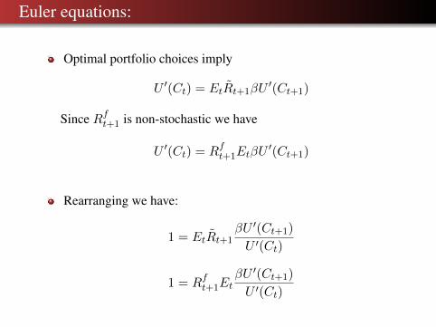
Optimal portfolio choices imply
U ′(Ct) = EtR̃t+1βU′(Ct+1)
Since Rft+1 is non-stochastic we have
U ′(Ct) = Rft+1EtβU′(Ct+1)
Rearranging we have:
1 = EtR̃t+1βU ′(Ct+1)
U ′(Ct)
1 = Rft+1EtβU ′(Ct+1)
U ′(Ct)

Risk Neutrality:
Constant U ′(C)
Euler equations imply:
EtR̃t+1 = Rft+1

General framework
Euler equation implies
Et {Mt+1Rt+1} = 1
where Mt+1 is pricing kernel and Rt+1 is the return.
Euler equation implies pricing kernel depends on consumption:
Mt+1 = βU ′(Ct+1)
U ′(Ct)
Implications
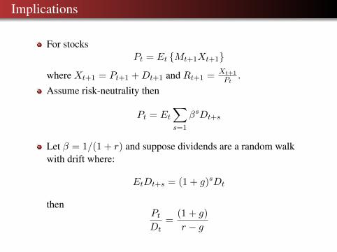
For stocksPt = Et {Mt+1Xt+1}
where Xt+1 = Pt+1 +Dt+1 and Rt+1 = Xt+1
Pt.
Assume risk-neutrality then
Pt = Et∑s=1
βsDt+s
Let β = 1/(1 + r) and suppose dividends are a random walkwith drift where:
EtDt+s = (1 + g)sDt
thenPtDt
=(1 + g)
r − g
Implications
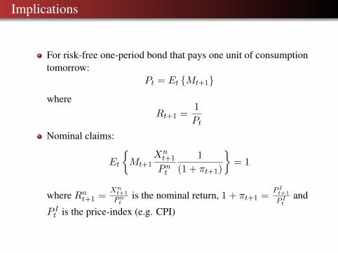
For risk-free one-period bond that pays one unit of consumptiontomorrow:
Pt = Et {Mt+1}
whereRt+1 =
1
Pt
Nominal claims:
Et
{Mt+1
Xnt+1
Pnt
1
(1 + πt+1)
}= 1
where Rnt+1 =Xnt+1
Pntis the nominal return, 1 + πt+1 =
P It+1
P Itand
P It is the price-index (e.g. CPI)

Consumption-Based Asset Pricing:
Equating the Euler equations gives:
Rft+1EtβU ′(Ct+1)
U ′(Ct)= EtR̃t+1
βU ′(Ct+1)
U ′(Ct)
Rearranging:(EtR̃t+1 −Rft+1
)EtβU ′(Ct+1)
U ′(Ct)= −COVt
(R̃t+1,
βU ′(Ct+1)
U ′(Ct)
)

Risk Premium
From Euler equation for risk-free asset
EtβU ′(Ct+1)
U ′(Ct)= 1/Rft+1
Therefore:(EtR̃t+1 −Rft+1
)Rft+1
= −COVt(R̃t+1,
βU ′(Ct+1)
U ′(Ct)
)

Implications:
If the risky return covaries positively with tomorrow’sconsumption, Ct+1, then the LHS is positive and the asset returnbears a positive premium over the risk free rate.
If the risky return covaries negatively with tomorrow’sconsumption then the LHS is negative and the asset return bearsa negative premium over the risk free rate.
Intuition: assets whose returns have a negative covariance withconsumption provide a hedge against consumption risk.Households are willing to accept a lower expected return sincethese assets provide insurance against low future consumption.

The equity premium puzzle:
Assume CRRA:
U(C) =C1−γ
1− γ
The Euler equations are:
C−γt = EtR̃t+1βC−γt+1
C−γt = Rft+1EtβC−γt+1

An approximation to the Euler equation:
Let xt+1 = ln(Ct+1)− ln(Ct), r̃t+1= ln(R̃t+1), the Eulerequation becomes:
1 = Rft+1βEt exp(−γxt+1)
1 = βEt exp(−γxt+1 + r̃t+1)
Assume that consumption growth and asset returns are jointlylog-normally distributed:[
xt+1
r̃t+1
]∼ N
([xt+1
r̄t+1
],
[σ2x,t+1, σ2x,r,t+1
σ2x,r,t+1, σ2r,t+1
])
If x ∼ N(x, σ2x) then X = exp(x) is log-normally distributedwith
E(X) = exp(x+1
2σ2)

Risk premium with log-normal distribution
The Euler equations becomes
1 = β exp
(−γxt+1 + r̄t+1 +
1
2var(−γxt+1 + rt+1)
)
1 = β exp
(−γxt+1 + rft+1 +
1
2var(−γxt+1)
)

Implications
Take logs and equate these equations:
r̄t+1 − rft+1 =1
2var(−γxt+1)−
1
2var(−γxt+1 + r̃t+1)
= −1
2σ2r + γcov(x, r̃)
Let r̄t+1 = E(log R̃t+1)) then logE(R̃t+1) = r̄t+1 + 12σ
2r
logEtRt+1 − logRft+1 = γcorr(x, r̃)σxσr

Quantitative implications:
The equity premium is:
logEtRt+1 − logRft+1 = γcorr(x, r̃)σxσr
In US data, σr = 0.167, σx = 0.036, corr(x, r̃) = 0.4 so
If γ = 1 we have logERt+1 − logRft+1 = 0.24%.
If γ = 10 we have logERt+1 − logRft+1 = 2.4%
If γ = 25 we have logERt+1 − logRft+1 = 6.0%

Additional Implications
If return variance and consumption variance are constant, excessreturn is unpredictable.
If consumption growth iid and Ct = Dt, price-dividend ratio is aconstant.
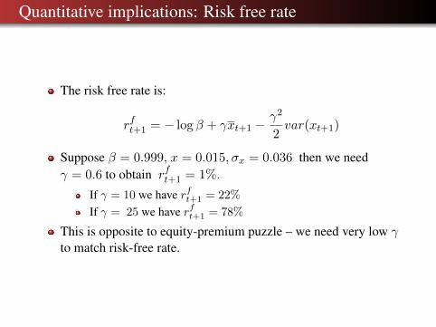
Quantitative implications: Risk free rate
The risk free rate is:
rft+1 = − log β + γxt+1 −γ2
2var(xt+1)
Suppose β = 0.999, x = 0.015, σx = 0.036 then we needγ = 0.6 to obtain rft+1 = 1%.
If γ = 10 we have rft+1 = 22%
If γ = 25 we have rft+1 = 78%
This is opposite to equity-premium puzzle – we need very low γto match risk-free rate.

Additional implications for risk free rate:
If consumption growth is iid and homoskedastic, then risk freerate is constant.
Risk free rate is high when expected consumption growth is high(intertemporal substitution).
Risk free rate is low when conditional consumption volatility islow (precautionary savings).
Consumption growth is close to iid but risk-free rates arepersistent.