University of Massachusetts Amherst ScholarWorks@UMass Amherst

CMPSCI 370: Intro to Computer VisionImage processing
[linear filtering]University of Massachusetts, Amherst
February 11, 2016
Instructor: Subhransu Maji
Slides credit: L. Lazebnik and others
• Homework 2 will be posted today • Will be due Tue., Feb. 23 before class • Questions on
• Linearity of light
• Color constancy
• Hybrid images — (today)
• Get started early
Administrivia
2
• What can we do to “enhance” an image after it has already been digitized? • We can make the information that is there easier to visualize. • We can guess at data that is not there, but we cannot be sure, in
general.
Enhancing images
3
contrast enhancement deblurring
Contrast stretching
4
histogram
before
afterimage source: wikipedia
map this to 255map this to 0

• How can we reduce noise in a photograph?
Motivation: Image de-noising
5
• Let’s replace each pixel with a weighted average of its neighborhood
• The weights are called the filter
• What are the weights for the average of a 3x3 neighborhood?
Moving average
6
111
111
111
“box filter”
Source: D. Lowe
• Let f be the image and g be the kernel. The output of convolving f with g is denoted f * g.
∑ −−=∗lk
lkglnkmfnmgf,
],[],[],)[(
Convolution
7Source: F. Durand
• MATLAB functions: conv2, filter2, imfilter
Convention: kernel is “flipped”
f
• Linearity: filter(f1 + f2) = filter(f1) + filter(f2)
• Scalars factor out: filter(k f1) = k filter(f1)
Some properties
8
What is the size of the output? • MATLAB: filter2(g, f, shape) or conv2(g, f, shape)
• shape = ‘full’: output size is sum of sizes of f and g • shape = ‘same’: output size is same as f • shape = ‘valid’: output size is difference of sizes of f and g
Annoying details
9
f
gg
gg
f
gg
gg
f
gg
gg
full same valid
What about near the edge? • the filter window falls off the edge of the image • need to extrapolate • methods:
- clip filter (black) - wrap around - copy edge - reflect across edge
Annoying details
10Source: S. Marschner
What about near the edge? • the filter window falls off the edge of the image • need to extrapolate • methods (MATLAB):
- clip filter (black): imfilter(f, g, 0) - wrap around: imfilter(f, g, ‘circular’) - copy edge: imfilter(f, g, ‘replicate’) - reflect across edge: imfilter(f, g, ‘symmetric’)
Annoying details
11Source: S. Marschner
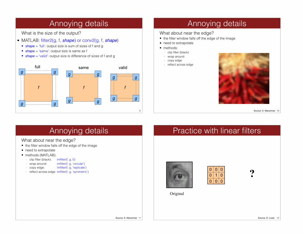
Practice with linear filters
12
000010000
Original
?
Source: D. Lowe
Practice with linear filters
13
000010000
Original Filtered (no change)
Source: D. Lowe
Practice with linear filters
14
000100000
Original
?
Source: D. Lowe
Practice with linear filters
15
000100000
Original Shifted leftBy 1 pixel
Source: D. Lowe
Practice with linear filters
16
Original
?111111111
Source: D. Lowe

Practice with linear filters
17
Original
111111111
Blur (with abox filter)
Source: D. Lowe
Practice with linear filters
18
Original
111111111
000020000 - ?
(Note that filter sums to 1)
Source: D. Lowe
Practice with linear filters
19
Original
111111111
000020000 -
Sharpening filter - Accentuates differences with local average
Source: D. Lowe
Sharpening
20Source: D. Lowe

• What’s wrong with this picture? • What’s the solution?
Smoothing with box filter revisited
21Source: D. Forsyth
• What’s wrong with this picture? • What’s the solution?
• To eliminate edge effects, weight contribution of neighborhood pixels according to their closeness to the center
Smoothing with box filter revisited
22“fuzzy blob”
• Constant factor at front makes volume sum to 1 (can be ignored when computing the filter values, as we should renormalize weights to sum to 1 in any case)
Gaussian Kernel
23Source: C. Rasmussen
• Standard deviation σ: determines extent of smoothing
Gaussian Kernel
24
σ = 2 with 30 x 30 kernel
σ = 5 with 30 x 30 kernel
Source: K. Grauman

• The Gaussian function has infinite support, but discrete filters use finite kernels
Choosing kernel width
25Source: K. Grauman
• Rule of thumb: set filter half-width to about 3σ
Choosing kernel width
26
Matlab command fspecial(‘gaussian’, hsize, sigma)
Gaussian vs. box filtering
27
• Salt and pepper noise: contains random occurrences of black and white pixels
• Impulse noise: contains random occurrences of white pixels
• Gaussian noise: variations in intensity drawn from a Gaussian normal distribution
Noise
28Source: S. Seitz

• Mathematical model: sum of many independent factors • Good for small standard deviations • Assumption: independent, zero-mean noise
Gaussian noise
29Source: M. Hebert
Smoothing with larger standard deviations suppresses noise, but also blurs the image
Reducing Gaussian noise
30
noise
What’s wrong with the results?
Reducing salt-and-pepper noise
31
3x3 5x5 7x7• A median filter operates over a window by selecting the
median intensity in the window
Alternative idea: Median filtering
32
• Is median filtering linear?Source: K. Grauman

• What advantage does median filtering have over Gaussian filtering? • Robustness to outliers
Median filter
33Source: K. Grauman
MATLAB: medfilt2(image, [h w])
Salt-and-pepper noise Median filtered
Source: M. Hebert
Median filter
34
What does blurring take away?
Sharpening revisited
35
original smoothed (5x5)
–
detail
=
sharpened
=
Let’s add it back:
original detail
+ k
α
Sharpening filter
36
Gaussianunit impulse
Laplacian of Gaussian
I = blurry(I) + sharp(I) sharp(I) = I � blurry(I)
= I ⇤ e� I ⇤ g�
= I ⇤ (e� g�)

A. Oliva, A. Torralba, P.G. Schyns, “Hybrid Images,” SIGGRAPH 2006
Application: Hybrid Images
37
Gaussian Filter
Laplacian Filter
39
motorcycle and bicycle
40
dolphin and car


![Ep118 Lec07 Polarization[1]](https://static.fdocuments.in/doc/165x107/563db822550346aa9a90d97b/ep118-lec07-polarization1.jpg)

![lec07 architecture.ppt [相容模式]](https://static.fdocuments.in/doc/165x107/623f9c6d3e8c6774d655d3d9/lec07-.jpg)