STAR*NET V6

Least Squares Survey Adjustment PackageTen-Station Demonstration Program

A Tour of

STAR*NETIncluding STAR*NET-PRO Features

STARPLUS SOFTWARE, INC.460 Boulevard Way, Oakland, CA 94610

510-653-4836

TOUR OF THE STAR*NET PACKAGE

Overview

STAR*NET performs least squares adjustments of 3D and three 3D survey networks.The standard edition handles networks containing conventional terrestrial observations.The professional edition adds the handling of GPS vectors plus full support for geoid andvertical deflection modeling during an adjustment. The software is menu driven andallows you to edit your input data, run your adjustment and view the adjustment results,both graphically and in a listing report, all from within the program.

Although STAR*NET is easy to use, it is also very powerful, and utilizes rigorousadjustment and analysis techniques. In 3D mode, it performs a simultaneous adjustmentof 3D data, not simply an adjustment of horizontal followed by an adjustment of vertical.STAR*NET is ideal for the adjustment of traditional interconnected traverse networks.It is equally suited to the analysis of data sets for establishing control for close-rangephotogrammetry and structural deformation monitoring.

This tutorial includes examples designed to acquaint you with the general capabilities ofthe STAR*NET and STAR*NET-PRO packages. It contains the following:

STAR*NET Demo Program Installation Instructions.

Example 1: Two dimensional traverse network. This example shows you the basicfeatures of STAR*NET, and lets you run an adjustment and view the output resultsin both listing and graphical formats.

Example 2: Combined triangulation/trilateration network.

Example 3: Three dimensional traverse network.

Example 4: Same three dimensional network, but processed as a grid job.

Example 5: Resection.

Example 6: Traverse with sideshots.

Example 7: Preanalysis of a network.

Example 8: Simple GPS network.

Example 9: Combining conventional observations and GPS vectors.

Supplemental information. Some extra details are included is you want to try outadditional STAR*NET features on your own using the demo program.

2

In this tutorial, we will go through the same sequence of operations that you wouldnormally follow when creating and adjusting a survey network – but in these examples,we will be just reviewing options and data, not setting options and creating new data.The normal sequence of operations one goes through in adjusting a survey project is thefollowing: set project options, create input data, run an adjustment, review resultsincluding viewing both an adjusted network plot and an output listing report.

The demo program is a fully functional version of STAR*NET. It includes all thecapabilities of the STAR*NET and STAR*NET-PRO editions, except that it is limited toan adjustment of 10 stations, 100 observations and 15 GPS vectors.

Note that this tutorial documentation is not designed to be an operating manual. It isintended only as a guide to the use of the demo program. A complete, fully detailedmanual is provided with purchase of STAR*NET. To order the program, or if you havequestions about its use, please contact:

STARPLUS SOFTWARE, INC.460 Boulevard Way, Oakland, CA 94610800-446-7848 sales and product information510-653-4836510-653-2727 (Fax)Email: starplus@earthlink.net

Installing the STAR*NET Demo Program

If you received diskettes, insert the Install Diskette #1 in your drive and go to Step 1.

If you downloaded (or were emailed) a single-file install program, simply double-clickthe file in explorer to start the installation, and go directly to Step 3.

1. From the Windows taskbar, select Start>Run. The Run windows appears.

2. In the Open field, type “A:\SETUP”, substituting the letter of the diskette drive ifyou use a drive other than drive “A”. Select OK.

3. Follow the installer instructions. Note that you can accept the default destinationdirectory named “C:\Program Files\Starplus\StarNet-Demo” or choose a differentdestination directory by browsing.

If you choose to designate a different installation destination, we encourage you tocreate a separate directory for the demo, not one already containing other programsfrom Starplus Software or other companies, to eliminate the possibility of conflicts.

4. After installing, press the Windows “Start” button, select Programs>Starplus, andthen click the “StarDemo” selection to run the STAR*NET demo program.

3

Example projects provided for this tutorial are located in a subfolder of your installdirectory named “Examples.” Therefore:

If you installed the demo in “C:\Program Files\Starplus\StarNet-Demo,” then,

The example projects are in “C:\Program Files\Starplus\StarNet-Demo\Examples.”

Each sample project consists of a “Project” file (a file with a “prj” extension) and at leastone “Data” file (a file with a “dat” extension). An existing project is opened by selectingits “prj” file from the Open Project dialogue.

The “Project” file contains all the option settings for a project such as whether it is a 2Dor 3D job, a local or grid job, all instrument standard error settings, and much moreinformation. The project file also includes a list of all data files that are considered partof the project. All options are preset for these sample projects, so you can simply reviewthem and not be concerned about setting or changing any yourself.

All “Data” files used in STAR*NET are simple text files that may be prepared within theprogram or external to the program using any text editor. All of the input data files forthe sample projects are provided, with full comments, to help you get an idea of how touse STAR*NET to handle your adjustment problems. It is not required that you edit anyof these sample data files when running the sample projects.

In the following examples in this tour, the instructions simply ask you to open a namedproject. Choose File>Open Project, or press the Open tool button, and the followingdialog will appear allowing you to open one of the existing example projects.

If for some reason the example projects as shown above do not appear, browse to thefolder you installed the STAR*NET demo, open the sub-folder named “Examples” andyou will find them there.

Note! For the sake of simplicity in this tutorial, the dialogues that show the path of theexample projects will indicate that the “Starplus” directory exists right at the root.

4

Example 1: Two Dimensional Traverse Network

The first example project demonstrates the functioning of STAR*NET's main menusystem. You will run an adjustment for a project, then view the results in both graphicaland listing formats. After running this example, you should have a basic understandingof how the program works. Later examples will show more data types and go into moredetail about program options.

# 2D Job with Multi-Loop Traverses # C 1 5045.572 5495.338 ! ! # fixed coordinates C 6 5000 5190 # approximate coordinates # TB 6 # traverse backsight to point 6 T 1 99-47-25 205.03 T 2 115-10-00 134.19 T 3 94-51-53 105.44 T 4 216-46-09 161.57 'Existing post T 5 106-26-42 160.71 'Iron pipe T 6 86-57-49 308.30 TE 1 # end this loop at Point 1 # TB 2 # traverse backsight to point 2 T 3 225-47-02 115.41 T 7 97-31-36 284.40 T 8 115-14-57 191.66 T 9 156-15-44 166.90 M 9-8-5 83-45-28 161.95 # add a tie-in course to 5 T 10 106-12-32 151.34 TE 6 164-00-42 1 # end at 6, turn angle into 1 # # fixed bearing B 8-7 n79-52-31e !

308.30

161.57

105.

44

205.

03

284.40

134.19

191.

6616

6.90

151.34

161.95

115.41

160.

71

N79-52-31E

100°

115°

217°

95°

225°

98°

106°156°

84°

115°

106° 87°164°

2

1

3

4

5

6

7

8

9

10

5

1. Run STAR*NET and open the “Trav2D.prj” example project.

2. The Main STAR*NET Menu will appear:

All program operations can be selected from these dropdown menus, and the mostcommon operations can be selected by pressing one of the tool-buttons. Pause yourmouse pointer over each button to see a short description of its function.

3. Choose Options>Project, or press the Project Options tool button.

The “Adjustment” options page includes important settings that describe the project,whether it is a 2D or 3D job, local or grid adjustment, linear and angular units used,and information about the datum scheme. Note that a realistic “Average ProjectElevation” should be entered if you are asking the program to reduce yourobservations to some common datum, but this is not the case in this sample job, sowe’ve left the value at zero. Other important calculations based on this averageproject elevation are described in the full manual.

Note that only relevant items on this options page are active. For example, othersections in this menu page and other pages will be active or inactive (grayed-out)depending on whether a job is 2D or 3D, or Local or Grid.

6

4. Review the “General” options by clicking the “General” tab. This page includessettings that are very general in nature that you seldom need to change during the lifeof a job. Some of these settings are actually “preferences” which describe the orderyou normally enter your coordinates (North-East, or visa versa), or the station nameorder you prefer when entering angles (At-From-To or From-At-To).

5. Review the “Instrument” options page. Here you see default values used in theadjustment, such as standard errors for each of the data type, instrument and targetcentering errors, and distance and elevation difference proportional (PPM) errors.These are some of the most important parameters in the program since they are usedin the weighting of your observation data.

7

Note that instrument and target centering errors can be included to automaticallyinflate the standard error values for distance and angle observations. Enteringhorizontal centering errors causes angles with “short sights” to be less important inan adjustment than those with “long sights.” Likewise, in 3D jobs, a verticalcentering error can also be included to cause zenith angles with short sights to be lessimportant in an adjustment than those with long sights.

6. Review the “Listing File” options page. These options allows you to control whatsections will be included in the output listing file when you run an adjustment. Notethat the Unadjusted Observations and Weighting item is checked. This causes anorganized review of all of your input observations, sorted by data type, to beincluded in the listing – an important review of your input.

The Adjusted Observations and Residuals section, is of course, the most importantsection since it shows you what changes STAR*NET made to your observationsduring the adjustment process – these are the residuals.

Note that the Traverse Closures section is also checked. This creates a nicelyformatted summary of your traverses and traverse closures in the listing. You’ll seethese and the other selected sections later in this tutorial project once you run theadjustment and then view the listing.

The last part of this options page allows you so set options that affect the appearanceof observations or results in the listing. Note that you can choose to have yourunadjusted and adjusted observation listing sections shown in the same order theobservations were found in your data, or sorted by station names.

You can also choose to have the adjusted observations listing section sorted by thesize of their residuals – sometimes helpful when debugging a network adjustment.

8

7. Finally, review the “Other Files” options page. This menu allows you to selectadditional output files to be created during an adjustment run. For example, you canchoose to have a coordinate points file created. Or when adjusting a “grid” job, youcan choose to have a geodetic positions file created.

The optional “Ground Scale” file is particularly useful then running grid jobs. Youcan specify that the adjusted coordinates (grid coordinates in the case of a grid job)be scaled to ground surface based on a combined scale factor determined during theadjustment, or a factor given by the user. These newly-created ground coordinatescan also be rotated and translated by the program.

The optional “Station Information Dump” file contains all information about eachadjusted point including point names, coordinates, descriptors, geodetic positionsand ellipse heights (for grid jobs) and ellipse information. The items are commadelimited text fields which can be read by external spread sheet and databaseprograms – useful for those wishing to create custom coordinate reports. This fileand the “Ground Scale” file are described in detail in the full manual.

The Coordinate Points and Ground Scaled Points files can both be output in variousformats using format specifications created by the user. The user-defined formattingspecifications are discussed in the full manual.

8. The “Special” option tab includes a positional tolerance checking feature to supportcertain government (such as ACSM/ALTA) requirements, but is not discussed in thistutorial. The “GPS” and “Modeling” option tabs are active in the “PRO” edition. Seethe last two examples in this tutorial for a description of the “GPS” options menu.

9. This concludes a brief overview of the Project Options menus. After you are finishedreviewing these menus, press “OK” to close the dialogue.

9

10. Our next step is to review the input data. Choose Input>Data Files, or press theInput Data Files tool button. In this dialogue you can add data files to your project,remove files, edit and view them, or rearrange their position in the list. The order ofthe list is the order files are read during an adjustment. You can also “uncheck” a fileto temporarily eliminate it from an adjustment – handy when debugging a largeproject containing many files. This simple project includes only one data file.

View the highlighted data file by pressing the “View” button. A view window opensso you can scroll through a file of any size. Take a minute to review the data andthen close the window when finished. To edit the file rather than view it, you wouldpress the “Edit” button, or simply double-click its name in the list.

Note that the Input Data dialogue automatically closes when you view or edit a file.Otherwise, for the other functions, you would press “OK” to exit the dialogue.

11. Run the adjustment! Choose Run>Adjust Network, or press the Run Adjustmenttool button. A Processing Summary window opens to show the progress.

When the adjustment finishes, a shortstatistical summary is shown in theprogress window indicating how eachtype of data fit the adjustment. Thetotal error factor is shown, and anindication whether the Chi SquareTest passed, a test on the “goodness”of the adjustment.

After adjusting a network, you willwant to view the plot, or review theadjustment listing.

We’ll view the network plot next.

10

12. To view the plot, choose Output>Plot, or press the Network Plot tool button.

Resize and locate the plot window for viewing convenience. The size and location ofmost windows in STAR*NET are remembered from run to run.

Experiment with the tool keys to zoom in and zoom out. Also zoom in to anyselected location by “dragging” a zoom box around an area with your mouse. Use the“Pan” tool to set a panning mode, and small hand appears as your mouse pointerwhich you can drag around to pan the image. Click the “Pan” tool again to turn themode off. Use the “Find” tool to find any point in a large network. Use the “Inverse”tool to inverse between any two points on the plot. Type names into the dialogue orsimply click points on the plot to fill them in (example above) and press Inverse.

Pop up a “Quick Change” menu by right-clicking anywhere on the plot. Use thismenu to quickly turn on or off items (names, markers, ellipses) on the plot.

Click the “Properties” tool button to bring up a plot properties dialogue to changemany plotting options at one time including which items to show, and sizingproperties of names, markers, and error ellipses.

Double-click any point on the plot to see its adjusted coordinate values and errorellipse dimensions. Double-click any line on the plot to see its adjusted azimuth,length, elevation difference (for 3D jobs), and relative ellipse dimensions.

Choose File>Print Preview or File>Print, or the respective tool buttons on theprogram’s mainframe tool bar, to preview or print a plot. More details using thevarious plot tools to view your network and printing the network plot are discussedin the full operating manual.

When you are finished viewing the adjusted network plot, let’s continue on andreview the output adjustment listing next.

11

13. To view the listing, choose Output>Listing, or press the Listing tool button.

The listing file shows the results for the entire adjustment. First, locate and size thelisting window large enough for your viewing convenience. This location and sizewill be remembered. Take a few minutes to scroll through the listing and review itscontents. For quick navigation, use the tool buttons on the window frame to jumpforward or backward in the file one heading at a time, a whole section at a time, or tothe end or top of the file.

For quicker navigation to any section in the file, right-click anywhere on the listing,or press the Index Tree tool button to pop up a “Listing Index” (as shown above).Click any section in this index to jump there. Click [+] and [-] in the index to openand close sections as you would in Windows Explorer. Relocate the index window toa convenient location it will stay. Check the “Keep on Top” box on the indexwindow if you want it to always be present when the listing is active.

Using one of the navigation methods described above, go to the section named“Summary of Unadjusted Input Observations.” Note that each observation has astandard error assigned to it. These are the default values assigned by the programusing the project options instrument settings reviewed earlier in step 5.

Still in the listing, further on, look at the “Statistical Summary.” This importantsection indicates the quality of the adjustment and how well each type of data suchas angles, distances, etc. fit into the overall adjusted network.

Always review the “Adjusted Observations and Residuals” section! It shows howmuch STAR*NET had to change each observation to produce a best-fit solution. Thesize of these residuals may pinpoint trouble spots in your network data.

12

Take a look at the “Traverse Closures of Unadjusted Observations” section. Thisproject had data entered in traverse form, and in the Project Options, this report wasselected as one of the sections to include in the listing. For each traverse, courses arelisted with unadjusted bearings (or azimuths) and horizontal distances. Whenpossible, angular misclosures are shown along with the amount of error per angle.The linear misclosures are shown based on unadjusted angles “corrected” by the per-angle error. Many governmental agencies want to see this kind of closure analysis.But it is important to note, however, that these corrections are only for the benefit ofthis traverse closure listing. Actual corrections to angles are calculated during theleast squares adjustment, and are shown as residuals.

At the end of the listing, review the Error Propagation listing section. You will findthe standard deviation values and the propagated error ellipse information for alladjusted stations. Also present are relative error ellipses between all station pairsconnected by an observation.

This concludes the quick review of the listing. You’ll note that much information isshown in this file – it contains just about everything you might want to know aboutthe results of an adjustment. In some cases, you may only wish to see a subset of thisinformation, so remember that you can tailor the contents of this file by selectingwhich sections to include in the Project Options/ Listing file menu.

14. In the “Project Options/Other Files” menu reviewed in step 7, an option was set tocreate an adjusted coordinates file. Choose Output>Coordinates to view this file.Any additional files created can also be viewed from this menu.

15. This completes the review of the “Trav2D” example project. We have toured themain option menus, the input data dialogue, performed an adjustment, reviewed theoutput listing contents in some detail and viewed network plots. Now that you have agood idea how the program works, the remaining tutorial examples can be examinedwith a minimum of explanation.

13

The sample project that you have just stepped through is a realistic example of a smalltwo dimensional multi-loop traverse. Note that only a few simple steps are required torun an adjustment:

Set options for your project Create one or more data files Run the adjustment Review both graphical and listing output

The “listing file” you reviewed by choosing Output>Listing is the final adjustmentreport produced from the STAR*NET run. Once a project is adjusted to yoursatisfaction, you would normally want to get a printout of this listing for your records.This file is a text file having the name of your project, plus a “lst” extension. A listingfile named “Trav3D.lst” therefore, was created by running this example.

The listing file can be printed from within the program by choosing File>Print while thelisting window is open and active.

The adjusted coordinates for this project are in a file named “Trav2D.pts” and like thelisting file, can be simply printed from within the program. Since the points are in textformat, many COGO programs will be able to read them directly.

However for your convenience, there is a “Points Reformatter” utility that can be runfrom the “Tools” menu. This utility allows export adjusted coordinates to severalstandard formats, as well as custom formats defined by you

Another utility available from the “Tools” menu is a “DXF Exporter” which creates anetwork plot in AutoCAD compatible DXF format.

STAR*NET offers many options and has extensive features not described in this tutorial,but in general, most adjustments can be performed in the straight forward fashionillustrated by this example. At this point, you may wish to go back and review the actualdata file used for this example. Note that the “Traverse” mode of data entry is very easyand efficient. Multiple traverses can be entered in one file, and additional distance andangle observations can be freely mixed with the traverse data, so as to keep observationsin the same order as your field book.

The remaining examples illustrate more STAR*NET capabilities and data types. It isassumed after following all the steps detailed in this first example project that you arenow somewhat familiar with the operation of the program. The following examples donot always go into detail describing the individual program functions.

14

Example 2: Combined Triangulation/Trilateration 2D Network

This example illustrates the adjustment of a simple triangulation-trilateration network. Inthe sample data file, many data lines are entered using the “M” code. This is the mostcommonly used data type meaning all “measurements” to another station. All theremaining independent observation are entered on a single “A” and “D” data lines.

# Combined Triangulation-Trilateration 2D Network # C 1 5102.502 5793.197 ! ! C 3 7294.498 6940.221 ! ! C 2 5642 7017 # # Angle and Distance Observations at Perimeter M 2-1-3 111-08-11 1653.87 M 2-1-6 77-24-52 1124.25 M 3-2-4 87-07-04 1364.40 M 3-2-6 40-58-15 951.92 4.0 .03 M 4-3-5 120-26-52 1382.49 M 4-3-6 44-14-21 983.86 M 5-4-1 110-34-04 1130.75 M 5-4-6 39-46-29 1493.54 M 1-5-2 110-43-40 1337.89 M 1-5-6 65-36-54 1548.61 # # Angles at Center Point A 6-5-4 64-01-01 A 6-4-3 89-36-55 A 6-3-2 105-18-27 A 6-2-1 57-28-12 # # Distance Cross-ties D 1-4 2070.76 D 2-5 2034.47

1337.89

1653

.87

1548

.61

1124.25

1364.4095

1.92

1382

.49

983.86

1130.75

1493.54

2070.76

2034.47

41°120°44 °

111°

40 °

111°

66 °

111°

77 °

105°

57 °44 °

64 °

90 °

87 °

4

1

2

3

5

6

15

1. Open the “Net2D.prj” example project.

2. Choose Input>Data Files, or press the Data Files tool button to open the Data Filesdialogue. Then press “View” to view the “Net2D.dat” example data file.

Note that the Measure lines contain horizontal angle and distance observations fromone station to another. The standard errors for observations normally default toInstrument setting values defined in the Project Options as discussed in the lastexample. However, for illustration purposes, explicit standard errors have beenadded to one of the data lines in this example. Close the view window.

3. Run the adjustment, by choosing Run>Adjust Network, or by pressing the RunAdjustment tool button.

4. Choose Output>Plot or press the Network Plot tool button to view the networkgraphically. Experiment by resizing the plot window larger and smaller by draggingthe corners or edge of the plot window.

5. Zoom into a section of the plot by dragging your mouse pointer around some part ofthe network. For example, drag a zoom box around just points 1 and 2. Note thestatus information at the bottom of the plot window. The North and East coordinatesare shown for the location of the mouse pointer as you move it around the plot. TheWidth value shown is the width of the plot window in ground units, FeetUS in thisexample. This width value will give you a good sense of scale when you are zoomedway into a very dense plot. Zoom out by pressing the Zoom All button.

Right-click anywhere on the plot to bring up the “Quick Change” menu. Click the“Show Relative Ellipses” item to make relative ellipses display. These ellipsesrepresent the relative confidences in azimuth and distance between connections inthe network. Double click any line and to see its adjusted azimuth and distancevalues plus its relative ellipse dimensions. Likewise, double click any point to see itsadjusted coordinates and ellipse dimensions. Chapter 8, “Analysis of AdjustmentOutput” in the full manual, includes an extensive discussion of error ellipse andrelative error ellipse interpretation.

6. View the Listing File by choosing Output>Listing, or by pressing the Listing toolbutton. Review the various parts of the listing in the same way you did for the lastexample. Be sure to review the “Statistical Summary” section which indicates howwell each group of observation types fit into the adjusted network.

Likewise, you should always review the “Adjusted Observations and Residuals”section which shows how much STAR*NET had to change your observations. Youwould normally examine this list carefully, especially if the adjustment fails the ChiSquare test, to look for possible problems with your data.

7. This completes the review of the “Net2D” example project.

16

Example 3: Three Dimensional Traverse Network

This example illustrates the adjustment of a three dimensional network. Data includestwo small traverses with slope distances and zenith angles. An extra cross tie is enteredbetween the two traverses. STAR*NET can also accept 3D data in the form of horizontaldistances and elevation differences.

# 3D Traverse Network#C A1 10000.00 10000.00 1000.00 ! ! !C A2 9866.00 7900.00 998.89 ! ! !

TE A2 # backsight to A2T A1 163-59-26.0 1153.67 91-35-30.0 5.25/5.30T 1 115-35-06.8 1709.78 90-56-41.6 5.31/5.32T 2 86-31-37.9 1467.74 90-05-56.2 5.26/5.31T 3 82-07-57.7 2161.76 88-20-39.6 5.15/5.22TE A1 75-45-17.6 1 # closing angle to 1

TB 1 # backsight to 1T 2 133-21-35.8 2746.28 91-37-53.3 4.98/5.12T 4 101-39-39.6 1396.76 88-23-31.8 5.23/5.25T 5 124-35-19.6 3643.41 88-28-02.3 5.35/5.30TE A2 80-48-52.2 A1 # closing angle to A1

M 5-4-3 69-59-28.7 2045.25 89-00-41.0 6.21/5.25

A1A2

1

2

3

4

5

1709.78

2746.28

1396.7

6

3643

.41

2045.25

1467.74

2161.76

1153.67

87°133°

102°

70°125°

81°

82°

164°76° 116°

17

1. Open the “Trav3D.prj” example project.

2. Take a look at the Project Options for this project. Note that on the Adjustmentoptions page the “Adjustment Type” is now set to 3D. On the same menu, down inthe Local Jobs group of options, we have the Default Datum Scheme set to “Reduceto a Common Datum” and the elevation value is set to 0.00 feet. What this means isthat we want the job reduced to sea level. The controlling coordinates given in thedata must be sea level values, and during the adjustment, observations will beinternally reduced to this datum to produce sea level coordinates.

Also while in the Project Options, review the “Instrument” settings page. Note thatall settings for vertical observations are now active. Centering errors of 0.005 feethave been set for both horizontal and vertical centering which will affect standarderrors for all our measurements. Shorter sightings will receive less weight!

3. Examine the input data file. Note that each traverse line now contains additional dataelements, the zenith angle and an “HI/HT” entry giving the instrument and targetheights. Coordinate lines now contain an elevation value. The sample data filecontains two small connecting traverses. The “TB” (traverse begin) lines indicate thebeginning backsights, and the “TE” (traverse end) lines indicate at which station thetraverses end. In this example, they both contain an optional closing angle.STAR*NET will use this information in the traverse closure listing, as well asentering them as observations in the adjustment.

Additional redundancy is provided by an “M” data line containing angle, distanceand vertical information between points on the two traverses.

4. Run the network adjustment and then look at the network graphically. Double clickany of the adjusted points and note the displayed information now includes adjustedelevations and vertical confidence statistics.

5. View the output Listing file. Review the unadjusted observations and note that thestandard errors for all angles and zenith angles are no longer constant values.Because of the “centering error” values entered in the instrument options, thestandard errors assigned to these observations will be larger (less weight) for angleswith short sights than for those with long sights.

Further down in the listing, review the adjustment statistical summary. Since this is a3D job, you now see additional items in this list. Review the remaining sections andnote the differences from the previous 2D adjustment listing in the first two exampleprojects. In the Traverse Closures section, for example, vertical traverse closures areshown. And in the Error Propagation section, standard deviations are shown forelevations, and vertical confidences for ellipses.

6. This completes the review of the “Trav3D” example project.

18

Example 4: Three Dimensional Grid Job

This example demonstrates the ability of STAR*NET to reduce ground observations to agrid system plane during the processing of a network adjustment.

The following example is the same 3D multiple traverse network illustrated in theprevious example. All ground observations are identical; only the coordinates have beenchanged to be consistent with NAD83, California Zone 0403.

# 3D Traverse Grid Job#C A1 2186970.930 6417594.370 300.00 ! ! !C A2 2186836.940 6415494.520 298.89 ! ! !#TB A2 # traverse backsight to A2T A1 163-59-26.0 1153.67 91-35-30.0 5.25/5.30T 1 115-35-06.8 1709.78 90-56-41.6 5.31/5.32T 2 86-31-37.9 1467.74 90-05-56.2 5.26/5.31T 3 82-07-57.7 2161.76 88-20-39.6 5.15/5.22TE A1 75-45-17.6 1 # closing angle to Station 1#TB 1T 2 133-21-35.8 2746.28 91-37-53.3 4.98/5.12T 4 101-39-39.6 1396.76 88-23-31.8 5.23/5.25T 5 124-35-19.6 3643.41 88-28-02.3 5.35/5.30TE A2 80-48-52.25 A1 # closing angle to Station A1

M 5-4-3 69-59-28.7 2045.25 89-00-41.0 6.21/5.25

A1A2

1

2

3

4

5

1709.78

2746.28

1396.7

6

3643

.41

2045.25

1467.74

2161.76

1153.67

87°133°

102°

70°125°

81°

82°

164°76° 116°

19

1. Open the “Grid3D.prj” example project.

2. Open the Project Options for this job and review the Adjustment options page. Youwill see some differences from the adjustment options in the last example project:

First, you will note that the Coordinate System is set to “Grid,” and the actual gridsystem chosen from the dropdown selection list is NAD83. Other selections areNAD27, UTM and Custom. (User-defined and international grids come under thecategory of Custom.) The zone currently selected, as indicated on the large selectionbutton, is California Zone 0403. How is a zone selected? Simply press the largeselection button to bring up the zone selection dialogue. Give it a try.

Here you just select from the list to change zones. Press “Show Parameters” to seethe zones parameters. Don’t make a new selection now – just press OK to exit.

20

Before you exit the Project Options, note another difference in the options from theprevious example. At the bottom of the menu is an options group specific to gridjobs. Here you enter the average Geoid Height. This value is always entered inmeters, and it is important to use the correct sign. (It’s negative in the contiguousUnited States.) You can also enter average deflections of the vertical due to gravity.Positive values are in north and east directions. These values can normally be left atzero, but if there are significant deflections in your project area (i.e. severalseconds), entering realistic values here should give you better results.

3. Examine the data file if you wish. As mentioned before, the observation data for thisexample is identical to the previous example except that the entered controlcoordinates are grid coordinates consistent with NAD83, California zone 0403. Thesame data set was used for this example so that, if you wish, you can compare outputresults from two identical jobs, one run as local, and the other as grid.

4. Run the network adjustment. Look at the network graphically – it will look the sameas in the last example. However, if you double click any of the adjusted points, thedisplayed coordinates will now, of course, be grid coordinates.

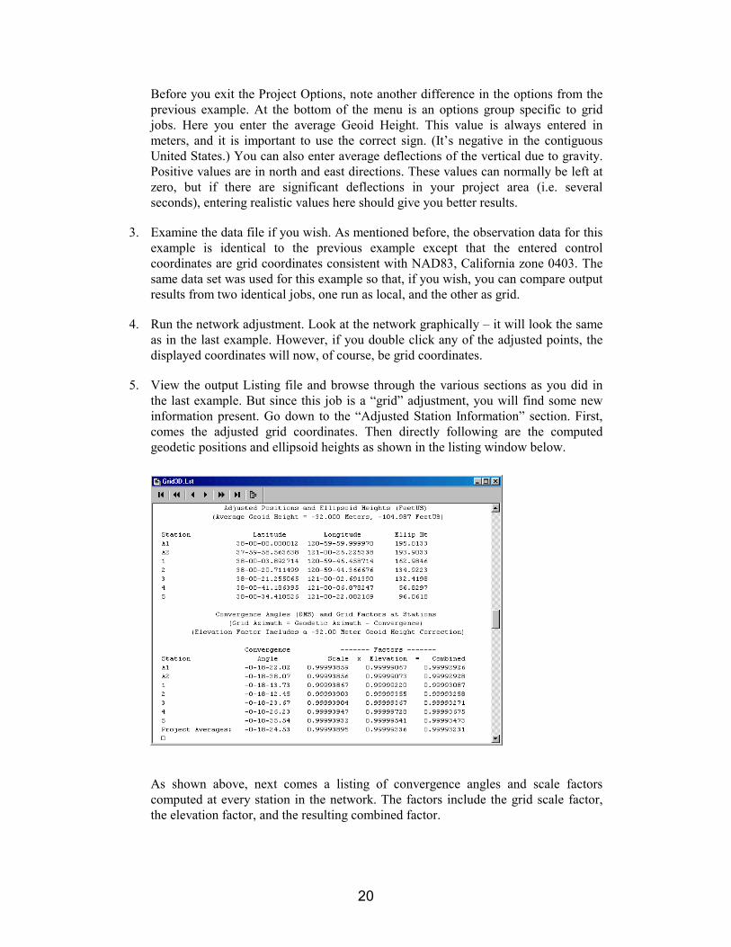
5. View the output Listing file and browse through the various sections as you did inthe last example. But since this job is a “grid” adjustment, you will find some newinformation present. Go down to the “Adjusted Station Information” section. First,comes the adjusted grid coordinates. Then directly following are the computedgeodetic positions and ellipsoid heights as shown in the listing window below.

As shown above, next comes a listing of convergence angles and scale factorscomputed at every station in the network. The factors include the grid scale factor,the elevation factor, and the resulting combined factor.

21

In the “Adjusted Bearings and Horizontal Distances” section previously seen in otherexamples in this tour, the bearing shown is now a “grid” bearing, and both “grid” and“ground” distances are now shown for every network connection.

Finally, look at the “Traverse Closures of Unadjusted Observations” section. Sincethis is a “grid” job, the listing of traverse closures is based on unadjusted bearingsand distances that are reduced to the grid plane.

6. See what other files were created by the adjustment by looking at the items that showup in the Output pulldown menu. Before we’ve seen the Coordinates file. And nowwe see a Lat/Longs (geodetic positions) file. The creation of both these files wererequested in the ”Project Options/Other Files” menu. Go ahead and view one or bothof these files if you want.

7. This completes the review of the “Grid3D” example project. Since this was the first“grid” job in our tutorial examples, we went into extra detail reviewing the optionsettings and output sections relating to grid adjustments.

22

Example 5: Resection

This example demonstrates the use of STAR*NET in solving a resection problem,involving the measurement of angles from 6 known stations to an unknown point.

# Resection

# Approximate location for the unknown station # C P48 104500 93600

# Fixed coordinates for the known stations # C 1 90132.03 88237.92 ! ! C 2 97418.58 82279.10 ! ! C 3 98696.21 81802.35 ! ! C 4 102911.40 80330.69 ! ! C 5 111203.37 95234.19 ! ! C 6 103278.43 106872.91 ! !

# Occupy “P48” and turn angles to known stations # A P48-1-2 37-35-00.0 A P48-2-3 5-56-19.4 A P48-3-4 19-56-18.3 A P48-4-5 115-34-35.0 A P48-5-6 78-09-31.0 A P48-6-1 102-48-30.0

103°

78°116°

38°

1

2

3

4

5

6

P48

23

1. Open the “Resection.prj” example project.

2. Review the project options if you wish. This is a standard 2D, local project.

3. Examine the input data file.

Note that all station coordinates are fixed with the “!” symbol, except for theunknown instrument station “P48” which is free. The angles default to the standarderror for angles set in the Project Options/Instrument options menu.

4. Run the adjustment.

Review the processing summary on the screen. Note that in the short statisticalsummary, the only observation type listed is the angle, and the adjustment passes theChi Square test.

5. Look at the network graphically.

You will see only one error ellipse since there is only one unknown point in thewhole network.

6. Review the listing file.

It’s quite short since our only observations are angles.

7. This completes the review of the “Resection” example project.

24

Example 6: Traverse with Sideshots

This example illustrates data consisting of a simple traverse containing many sideshots.Sideshots are diverted during loading of the input data file, and are not processed untilafter the network is adjusted. Their computed coordinates are written to both the ListingFile and the Points File. Because they are processed after the adjustment, no errorpropagation is performed on Sideshots. The sideshot data type is available so that youcan process a network containing hundreds or thousands of sideshots without slowingdown the adjustment of the actual network. In particular, this approach lends itself to theprocessing of large topo data sets downloaded from data collectors.

# Traverse with Sideshots # C 1 1000.00 1000.00 1440.28 ! ! ! C 2 1725.18 1274.36 1467.94 ! ! ! # # Begin Field Observations # TB 2 T 1 51-59-30 242.42 88-44-35 5.25/5.30 T 59 198-19-55 587.14 89-39-40 5.30/5.50 'IRON PIN T 572 140-52-34 668.50 80-14-25 5.18/5.22 TE 828 # # Begin Sideshots # SS 1-2-3 104-18-07 146.08 90-56-54 5.25/5.33 'TOE SS 1-2-4 24-33-33 118.64 89-16-07 5.25/5.33 'TOE SS 1-2-5 339-20-11 254.12 88-03-45 5.25/5.33 'FACE OF CURB SS 1-2-14 339-35-31 383.90 88-33-17 5.25/5.33 'TOE etc...

828

57259

2

1

25

1. Open the “Sideshots.prj” example project.

2. View the input data file. Note that the sideshots are entered with the “SS” code.Scroll down and view the entire file; the data includes quite a number of sideshots!Most of the sideshots also have a text descriptor at the end of the line, which ismarked with a single or double quote character.

Remember that the sideshots are processed after the adjustment, and do not slowdown the network processing. It is also important to remember that since sideshotsare not actually part of the “adjusted” network, and that you cannot occupy asideshot, or backsight to one. You cannot take a sideshot to the same point andexpect that point to be adjusted. In all these cases, you should enter yourobservations with an “M” data line which is included in the actual adjustment.

For simplicity, sideshots in this example were all entered following the traverse.However they may be freely intermixed with traverse data or any other types of data,to preserve the same order recorded in your field book or data collector.

3. Run the adjustment. The adjustment of the traverse proceeds very quickly, and thesideshots are processed independently after the adjustment is completed.

Note that in this particular example, the main traverse is simply an open endedtraverse that doesn't even tie into a known station. So in this case, although all pointsare computed, nothing is really adjusted. This illustrates how STAR*NET can beused simply as a data reduction tool. And had we been working in some gridcoordinate system, for example NAD83 or UTM, all the observations would havealso been reduced to grid, producing adjusted grid coordinates.

4. View the resulting network graphically - many sideshots fill the plot screen. Zoominto a small group of sideshots. Right-click the plot screen to bring up the QuickChange menu, and click the “Show Sideshot Descriptors” item to turn on viewing ofdescriptors. Descriptors often clutter up a plot view, so by default you will usuallyleave them turned off. You can also turn sideshots off and on in the Quick Changemenu by unchecking and checking the “Show Sidehots” item.

5. Take a quick look at the adjustment listing file. Looking through the listing you willsee a review of the input sideshot observation data as well as final sideshotcoordinates in the “Sideshot Coordinates Computed After Adjustment” section.These computed sideshot coordinates, along with the traverse coordinates, alsoappear in the “points” output file created during the processing. This file can beviewed by choosing Output>Coordinates as illustrated in earlier examples.

6. This completes the review of the “Sideshots” example project.

26

Example 7: Preanalysis

This example demonstrates using STAR*NET in the preanalysis of survey networks.Preanalysis means that the network will be solved using approximate coordinates tolocate the stations, and a list of observation stations to indicate which distances andangles are planned to be observed. No actual field data are required. STAR*NET willanalyze the geometric strength of the network using the approximate layout, and theinstrument accuracies supplied as observation standard errors. The predicted accuracy ofeach station will be computed, and error ellipses generated. Preanalysis is a powerfultool that will help you to test various network configurations before any field work isdone, or to test the effects of adding measurements to an existing network.

You can use any of the 2D and 3D data types provided for in STAR*NET to define aproposed survey. In this simple 2D example, we traverse around the perimeter, usemeasure lines to define some cross ties, and then fill in some angles.

# Preanalysis # C 1 51160 52640 ! ! C 2 50935 52530 C 3 50630 53660 C 1001 51160 52950 C 1002 51145 53280 C 1003 50645 53265 C 1004 50915 53570 C 1005 50655 52770 C 1006 50945 52820 C 1007 50865 53160 # B 1-2 ? ! #B 1003-3 ? 5.0 # Uncomment this line to add another bearing # TB 2 T 1 T 1001 T 1002 T 1004 T 3 T 1003 T 1007 T 1006 T 1005 T 2 TE 1 # M 1-2-1005 M 1-2-1006 M 1001-1-1006 M 1001-1-1007 M 1002-1001-1007 M 1002-1001-1003 M 1004-1002-1003 A 1003-1007-1002 A 1003-1007-1004 A 1007-1006-1001 A 1007-1006-1002 A 1006-1005-1 A 1006-1005-1001 A 1005-2-1

1 10011002

1004

31003

1007

1006

1005

2

27

1. Open the “Preanalysis.prj” example project. This is a “2D” project.

2. View the input data file. Note that all stations have been given approximatecoordinates. This defines the network geometry. Note also that the list of distanceand angle data lines contains no field observations. Observation standard errorsdefault to the values set for the various data types in the Project Options/Instrumentmenu. If a specific standard error is required, a place holder such as “?” is requiredon the data line in place of the actual observation.

3. Run the preanalysis by choosing Run>Preanalysis. Note that if you were to makeany other choice from the Run Menu such as “Adjust Network” or “Data CheckOnly,” errors would result due to the missing observations.

4. View the network graphically. Note that the resulting station error are larger for thestations furthest from the fixed station. Also, their shape and orientation suggest anazimuth deficiency in the network. This is the purpose of running a preanalysis, tostudy the strength of your planned survey network using only proposed fieldobservations.

5. If you wish, you can experiment with adding another observation to the network.Open the Data Files dialogue by choosing Input>Data Files, or by pressing theInput Data Files tool button. Press the ”Edit” button, or simply double-click thehighlighted data file in the list. Locate the line in the data file that has a Bearing fromStation 1003 to Station 3. Uncomment the line by deleting the “#” symbol at thebeginning of the line, just before the “B” code. Note that this data line has anexplicitly entered standard error of 5 seconds. (This new data, for example, mightrepresent an observed solar azimuth.) Save the file and exit from the text editor.

Now rerun the preanalysis by choosing Run>Preanalysis again. Review the newresults graphically as described in Step 4 above. Notice the increased positionalconfidence provided by the addition of the proposed bearing observation. Theellipses we were concerned with are now smaller and more round. If you wish to seethe actual ellipse dimensions, double-click any point on the plot, or of course youcan view the error ellipse information in the listing file as suggested below.

6. Take a quick look through the listing. Even though no actual observations wereprovided as input, observation values (angles and distances) will be shown in thelisting. These values are inversed from the given coordinates and standard errors areassigned to these proposed observations from the Project Options/Instrument menusettings. And of course, station ellipses and relative ellipses are also shown, theircomputed values being the main purpose for making a preanalysis run.

7. This completes the review of the “Preanalysis” example project.

28

Example 8: Simple GPS Network

This example demonstrates the major steps you would go through to setup and adjust asimple network made up of only GPS vectors. You will set a few required projectoptions, review the main data file which defines the coordinate constraints, import a fewvectors from Trimble GPSurvey baseline files, and adjust the network.

# Simple GPS Network# Fully-constrained, two fixed stations plus a fixed elevation

# Grid Coordinates are used for constraints in this example

C 0012 230946.1786 120618.7749 224.299 ! ! ! 'North RockC 0017 218691.2153 131994.0354 209.384 ! ! ! '80-1339E 0013 205.450 ! 'BM-9331

0012

0016

0018

0017

0015

0013

29

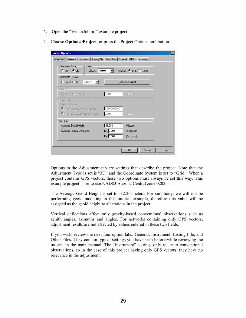
1. Open the “VectorJob.prj” example project.

2. Choose Options>Project, or press the Project Options tool button.

Options in the Adjustment tab are settings that describe the project. Note that theAdjustment Type is set is “3D” and the Coordinate System is set to “Grid.” When aproject contains GPS vectors, these two options must always be set this way. Thisexample project is set to use NAD83 Arizona Central zone 0202.

The Average Geoid Height is set to -32.20 meters. For simplicity, we will not beperforming geoid modeling in this tutorial example, therefore this value will beassigned as the geoid height to all stations in the project.

Vertical deflections affect only gravity-based conventional observations such aszenith angles, azimuths and angles. For networks containing only GPS vectors,adjustment results are not affected by values entered in these two fields.

If you wish, review the next four option tabs: General, Instrument, Listing File, andOther Files. They contain typical settings you have seen before while reviewing thetutorial in the main manual. The “Instrument” settings only relate to conventionalobservations, so in the case of this project having only GPS vectors, they have norelevance in the adjustment.

30

3. Review the “GPS” options by clicking the “GPS” tab. These fields allow you to setdefault values or options relating to GPS vectors present in your network data.

A value of 8.00 has been set for the “Factor Vector StdErrors” field which meansthat all the imported vector standard errors will be multiplied by this factor. Standarderrors reported by many baseline processors are over-optimistic and this optionallows you to make them more realistic. A “Vector Centering StdError” value of0.002 meters has been entered which further inflates the standard errors.

The “Transformations” box is checked and a choice has been made to solve for scaleand three rotations, around North, East and Up axes, during the adjustment. Solvingfor these transformations often helps “best-fit” vectors to your station constraints byremoving systematic errors or biases that may exist in vector data.

Finally, in the “Listing Appearance” options, certain output preferences are set forvarious listing items including how you like to see vector weighting expressed andhow both unadjusted and adjusted vectors data should be sorted. Note that in thissections, it has been chosen to show a “Residual Summary” section in the listing.We’ll review this very useful report later.

4. Review the “Modeling” tab. It is here that you select to perform both geoid modelingand deflection modeling during an adjustment. For simplicity in this demo tutorial,we are not going to perform any modeling. The average geoid height specified on theAdjustment options page will be applied to all stations in the network.

5. This concludes the overview of the Project Options for this example. After you arefinished reviewing the options, press “OK” to close the dialogue.

31

6. Next, review the input data. Choose Input>Data Files, or press the Input data toolbutton. Note there are two files in the list. The first file is the main data file shown atthe beginning of this example. It simply contains two stations with fixed north, eastand elevation values, and one station with a fixed elevation.

The second file contains the imported vectors for this project. For simplicity, wehave already imported the vectors into a file for this example, and it appears in thedata file list with the same name as the project, and with a “GPS” extension. In thenext step, we’ll actually go through the exercise of running the GPS importer toshow you how this file was created.

But while we are still in the Data Files dialogue, let’s review the vector file.Highlight the “VectorJob.Gps” file in the list and press the “View” button.

The file contains eight imported vectors. Each vector consists or four lines whichincludes a vector ID number, the Delta-X, Y & Z vector lengths, and covarianceinformation for weighting. After reviewing the vector data, close the window.

32

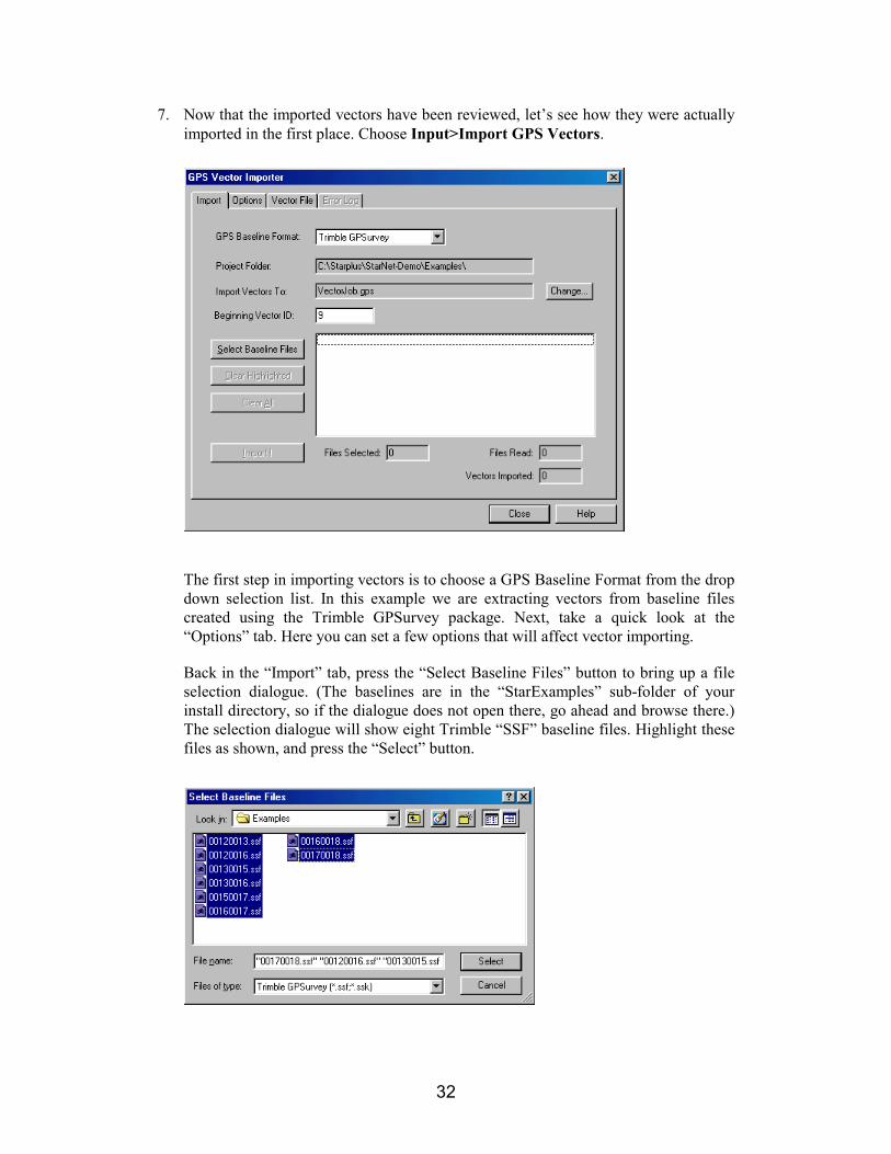
7. Now that the imported vectors have been reviewed, let’s see how they were actuallyimported in the first place. Choose Input>Import GPS Vectors.

The first step in importing vectors is to choose a GPS Baseline Format from the dropdown selection list. In this example we are extracting vectors from baseline filescreated using the Trimble GPSurvey package. Next, take a quick look at the“Options” tab. Here you can set a few options that will affect vector importing.

Back in the “Import” tab, press the “Select Baseline Files” button to bring up a fileselection dialogue. (The baselines are in the “StarExamples” sub-folder of yourinstall directory, so if the dialogue does not open there, go ahead and browse there.)The selection dialogue will show eight Trimble “SSF” baseline files. Highlight thesefiles as shown, and press the “Select” button.

33

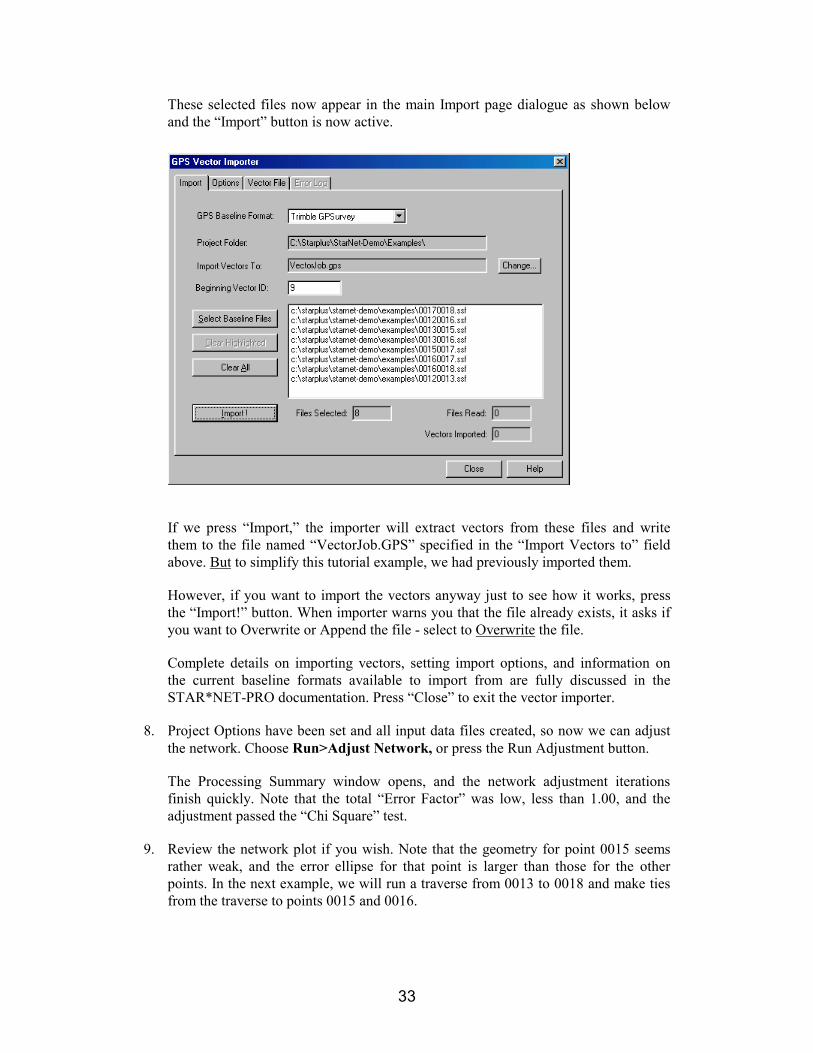
These selected files now appear in the main Import page dialogue as shown belowand the “Import” button is now active.

If we press “Import,” the importer will extract vectors from these files and writethem to the file named “VectorJob.GPS” specified in the “Import Vectors to” fieldabove. But to simplify this tutorial example, we had previously imported them.

However, if you want to import the vectors anyway just to see how it works, pressthe “Import!” button. When importer warns you that the file already exists, it asks ifyou want to Overwrite or Append the file - select to Overwrite the file.

Complete details on importing vectors, setting import options, and information onthe current baseline formats available to import from are fully discussed in theSTAR*NET-PRO documentation. Press “Close” to exit the vector importer.

8. Project Options have been set and all input data files created, so now we can adjustthe network. Choose Run>Adjust Network, or press the Run Adjustment button.

The Processing Summary window opens, and the network adjustment iterationsfinish quickly. Note that the total “Error Factor” was low, less than 1.00, and theadjustment passed the “Chi Square” test.

9. Review the network plot if you wish. Note that the geometry for point 0015 seemsrather weak, and the error ellipse for that point is larger than those for the otherpoints. In the next example, we will run a traverse from 0013 to 0018 and make tiesfrom the traverse to points 0015 and 0016.

34

10. View the output Listing file and browse through the various sections, especially theoutput sections relating to GPS vectors. Go to the “Summary of Unadjusted InputObservations” section where you will first see the list of controlling coordinates.

Directly following will be the unadjusted vectors showing the lengths and standarderrors of the Delta X, Y and Z components of each vector expressed in the earth-centered Cartesian system. Standard errors shown for these components include theaffects of any “Factoring” and “Centering Errors” set in the options.

Next go to the “Adjusted Observations and Residuals” section. The first part of thissection shows solutions of the transformations requested in the GPS optionsreviewed earlier. Here you see solutions for a scale and three rotations. The scalechange is very small as are the three rotations. This should be expected whenperforming an adjustment on a GPS-based ellipsoid such as WGS-84 or GRS-80. Ifany of these solved transformation values are unreasonably large, you need to reviewyour observations and constraints and find the reason why.

As shown above, the next output in the same section are the adjusted GPS vectorsand their residuals. Always review this important section since it shows you howmuch STAR*NET had to change each vector to produce a best-fit solution.

Note that all the vector, residual and standard error components have been rotatedfrom earth-centered Cartesian to local-horizon North, East and Up components. Thisorientation is simple to understand and very easily related to conventionalobservations.

35

The next section is the “GPS Vector Residual Summary” mentioned earlier in thisexample. Users find this one of the most helpful GPS related sections in the listing. Itcan be sorted in various ways to help you find the “Worst” vectors in your network.In our example, the summary is sorted by “3D” residuals, made up of local-horizonNorth, East and Up residual components.

Review the remaining sections in the listing file if you wish. These section are notunique to GPS vectors, and you have seen them before when running the examplesearlier in this tutorial.

11. This completes the “VectorJob” example project. This was a realistic example of asmall GPS job containing only vectors.

To keep the tutorial short however, this example skipped a very important step!When running your own adjustments, always run a minimally-constrainedadjustment first, holding only a single station fixed. This will test the integrity of theobservations without the influence of external constraints. When you are confidentthat all observations are fitting together well, then add any remaining fixed stationsto the network.

The next example will add the vectors from this project to some conventionalobservations and you will run a combined network adjustment. If you want tocontinue on to the next example, turn the page for instructions.

36

Example 9: Combining Conventional Observations and GPS

This example demonstrates combining conventional observations and GPS vectors in asingle adjustment. We'll be using the same imported vectors and constraints as in the lastexample, only now a traverse and some ties have been added to the network.

# Combining Conventional Observations and GPS Vectors# Latitudes and Longitudes are used as constraints in this example# The "VectorJob.GPS" file is added in the Data Files Dialogue

P 0012 33-04-44.24402 112-54-36.04569 224.299 ! ! ! 'North RockP 0017 32-58-09.73117 112-47-13.55717 209.384 ! ! ! 'AZDOT 80-1339E 0013 205.450 ! 'BM-9331

TB 0012T 0013 67-58-23.5 4013.95 90-04-44 5.35/5.40T 0051 160-18-01.7 2208.27 90-14-33 5.40/5.40T 0052 213-47-22.1 2202.07 89-43-20 5.36/5.40 'SW BridgeT 0053 198-52-17.3 2714.30 89-58-19 5.35/5.38TE 0018

# Ties to GPS pointsM 0051-0013-0015 240-35-47.03 1601.22 90-27-52 5.40/5.40M 0052-0051-0015 320-50-46.25 2499.61 90-05-49 5.36/5.41M 0052-0051-0016 142-02-01.50 2639.68 90-07-37 5.36/5.40M 0053-0052-0016 61-14-43.77 2859.65 90-20-19 5.35/5.42

0012

0016

0018

0017

0015

0013

0051

0052

0053

37

1. Open the “VectorCombined.prj” example project.

2. Review the Project Options if you wish. Since this project contains conventionalobservations, the “Instrument” options settings will be relevant in the adjustment.Note that the standard error values entered for the turned angle, distance and zenithangle observations are quite small indicating that high quality instruments and fieldprocedures are being used. The “GPS” option settings are the same as in the firstexample project.

When combining conventional observations with GPS vectors, it is particularlyimportant to carefully set weighting parameters in the Instrument options as well asin the GPS options since standard errors determine the relative influence of eachtype of data in the adjustment.

3. Open the Input Data Files dialogue. There are two files in the list. The first filenamed “VectorCombined.Dat” contains the station constraints and conventionalobservations, and the second file named “VectorJob.Gps” contains GPS vectorsimported to that file in the last example project. This file was simply added to thedata file list by pressing the “Add” button and selecting the file. View either of thesefiles if you wish, otherwise press “OK” to exit the dialogue.

Note that in the “VectorCombined.Dat” file contents shown on the first page of thisexample, the same stations have been constrained as were in the last project, exceptthey are entered as equivalent geodetic positions rather than grid coordinates simplyto illustrate use of that data type. Results will be identical either way.

Conventional observations in the network include a traverse and four ties fromtraverse stations to two of the GPS stations. The traverse lines and the tieobservations (the “M” lines) include turned angles, slope distances and zenith angles.Instrument and target heights are also included.

38

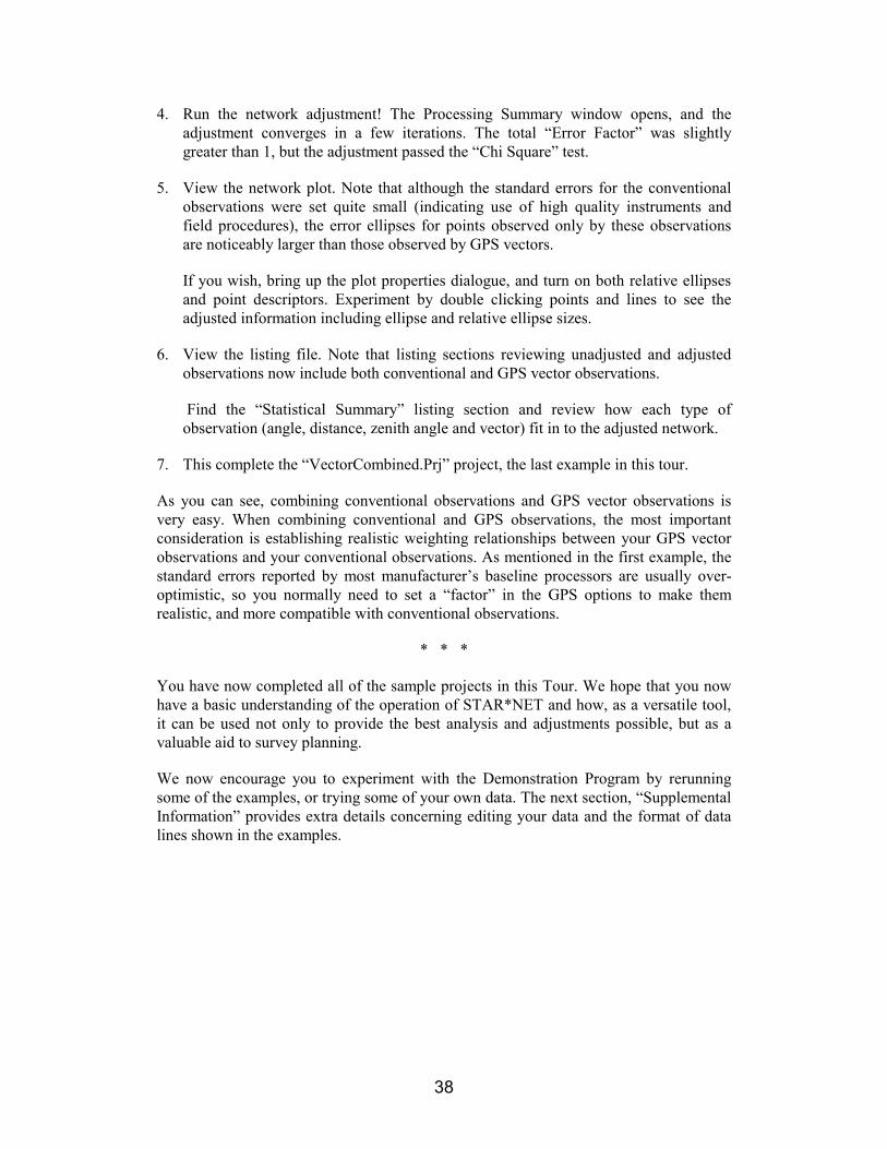
4. Run the network adjustment! The Processing Summary window opens, and theadjustment converges in a few iterations. The total “Error Factor” was slightlygreater than 1, but the adjustment passed the “Chi Square” test.

5. View the network plot. Note that although the standard errors for the conventionalobservations were set quite small (indicating use of high quality instruments andfield procedures), the error ellipses for points observed only by these observationsare noticeably larger than those observed by GPS vectors.

If you wish, bring up the plot properties dialogue, and turn on both relative ellipsesand point descriptors. Experiment by double clicking points and lines to see theadjusted information including ellipse and relative ellipse sizes.

6. View the listing file. Note that listing sections reviewing unadjusted and adjustedobservations now include both conventional and GPS vector observations.

Find the “Statistical Summary” listing section and review how each type ofobservation (angle, distance, zenith angle and vector) fit in to the adjusted network.

7. This complete the “VectorCombined.Prj” project, the last example in this tour.

As you can see, combining conventional observations and GPS vector observations isvery easy. When combining conventional and GPS observations, the most importantconsideration is establishing realistic weighting relationships between your GPS vectorobservations and your conventional observations. As mentioned in the first example, thestandard errors reported by most manufacturer’s baseline processors are usually over-optimistic, so you normally need to set a “factor” in the GPS options to make themrealistic, and more compatible with conventional observations.

* * *

You have now completed all of the sample projects in this Tour. We hope that you nowhave a basic understanding of the operation of STAR*NET and how, as a versatile tool,it can be used not only to provide the best analysis and adjustments possible, but as avaluable aid to survey planning.

We now encourage you to experiment with the Demonstration Program by rerunningsome of the examples, or trying some of your own data. The next section, “SupplementalInformation” provides extra details concerning editing your data and the format of datalines shown in the examples.

39

Supplemental Information

Editing Your Data

As illustrated in the tutorial, STAR*NET uses standard text files for all data. You cancreate and edit these data these files external to STAR*NET, or more conveniently, rightfrom the Data Files dialogue by highlighting a file name and pressing “Edit.”

When you installed the STAR*NET demo program, the windows “Notepad” editor wasassigned as the default editor. However, if you have a text editor you would rather haveSTAR*NET to use, choose File>Set Editor to make the change:

Browse for the editor of your choice and press OK. Note that you should normallyrefrain from using most word processors since they often insert special formattingcharacters that cannot be correctly interpreted by the STAR*NET program.

Input Data Files

This section is included for users of the STAR*NET Demo Program who want to changethe sample input data files, or create their own files. More detailed information may befound in the STAR*NET User's Manual, which is supplied with the purchase of the fullSTAR*NET or STAR*NET-PRO package.

STAR*NET input data files are standard text that can be created with a text editor. Datafiles can also be generated as output from some another program, such as a third partyCOGO program or a data collector routine. For example, Starplus Software hasdeveloped several utility programs which convert from raw field files (TDS, SDR33,SMI, etc.) to formats used in STAR*NET. Therefore, you might often create a data fileexternal to the program, and use the editing feature in STAR*NET to modify the file asneeded. However, you can also create the entire file by hand-typing observation datafrom within the program.

Although STAR*NET is flexible on how you can name your data files, it is suggestedthat you use “DAT” extensions for files consisting of conventional observations andcontrol coordinates, and “GPS” for imported vectors. For convenience, the programautomatically adds these extensions unless you specify otherwise. For example, if youcreate a project named “SouthPark”, the program will offer “SouthPark.dat” as a data filename in the Data Files dialogue.

40

Several files are created during an adjustment run. Each is given the project name, but adifferent extension. Using the “SouthPark” example project name, some of the outputfiles created will be SouthPark.lst, (adjustment results listing), SouthPark.pts (adjustedcoordinate points), SouthPark.pos (adjusted geographical positions if the job was grid),SouthPark.gnd (if you requested a ground-scale coordinates file to be created), etc.

Data Lines

STAR*NET input data files are relatively free in format. Spacing on a line is up to you,but the order of data elements on a line must conform to STAR*NET's rules. Generally,lines begin with a one or two alphabetic character code identifying the type of data,followed by the station names and actual observations. You have seen many examples ofthese data lines in the example projects.

For a least squares adjustment to work, coordinates (fixed or approximate) must beknown for all stations in the network. Fortunately STAR*NET has the ability to lookthrough all your data and figure out the approximate coordinates based on the actualangle and distance observation information in the data file. Often, however, you willhave to enter an approximate coordinate or two to help STAR*NET get startedcalculating other approximate coordinates. For example, in the first sample project onpage 4, we gave an approximate coordinate value for the first traverse backsight point.This is discussed in detail in the full STAR*NET User's Manual.

All STAR*NET data lines follow the same general format, as shown below.

Code Stations Observations Standard Errors

The first one or two characters of a line of data form the code that defines the content ofthe line. Next comes the station name(s), followed by the observation(s) and the standarderror(s). As explained in the STAR*NET User's Manual, the standard errors are used todefine how much importance (weight) a particular observation will have in theadjustment. Normally, you would simply set default standard errors for a project, and notinclude them on your data lines.

The line below defines a single distance observation with an explicit standard error:

D TOWER-822 932.66 0.03

Likewise, the line below defines a full set of 2D measurements, angle and distance, fromone point to another plus the respective standard errors:

M P25-12-HUB 163-43-30 1297.65 4 0.03

41

The following table lists data types in the STAR*NET and STAR*NET-PRO packages.These codes may be entered in upper or lower case.

Code Meaning

# Remainder of line is a comment and is ignored

C or CH Coordinate values for a station

E or EH Elevation value for a station

P or PH Geodetic Position for a station (Grid jobs only)

A Turned Angle

D Distance

V Zenith Angle or Elevation Difference (3D data only)

DV Distance and Vertical (3D Data only)

B Bearing or Azimuth

M Measure (Observations to another network point)

BM Bearing Measure (Observations to another network point)

SS Sideshot (Observations to a sideshot point)

TB Traverse Begin

T Traverse (All observations to next network point)

TE Traverse End

DB Begin Direction Set

DN Direction

DM Direction with Measure Data

DE End Direction Set

LW Define Differential Leveling Weighting

L Differential Level Measurement

G GPS Vector (Professional Edition)

GH Geoid Height Value (Professional Edition)

GT Vertical Deflection Value (Professional Edition)

Note that to keep this tutorial somewhat short and easy to review in a reasonable amountof time, all data type codes have not been illustrated in the example projects. The fullSTAR*NET manual along with the STAR*NET-PRO edition supplement fully describesand illustrates all data types shown here.

42

Following the data type code on a line of data is the name of one, two or three stationsdepending on the type of data line being entered. Multiple names are separated by a dash.In the distance line shown on page 40, “TOWER-822” defines the FROM and TOstations of the distance observation. Station names may be 1 to 15 characters in length,although only 10 characters are shown in most of the reports.

Next comes the actual observation (or observations) such as a distance, turned angle,zenith, azimuth or bearing, a direction, or coordinates for a station. Angular values maybe entered in “D-M-S” format (123-44-55.66) or “packed” format (123.445566), theformat commonly used by calculators. Angles may also be entered in GONS. Forsimplicity, all examples in this tutorial are shown entered in “D-M-S” format.

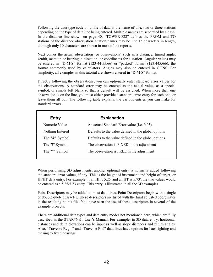
Directly following the observations, you can optionally enter standard error values forthe observations. A standard error may be entered as the actual value, as a specialsymbol, or simply left blank so that a default will be assigned. When more than oneobservation is on the line, you must either provide a standard error entry for each one, orleave them all out. The following table explains the various entries you can make forstandard errors.

Entry Explanation

Numeric Value An actual Standard Error value (i.e. 0.03)

Nothing Entered Defaults to the value defined in the global options

The "&" Symbol Defaults to the value defined in the global options

The "!" Symbol The observation is FIXED in the adjustment

The "*" Symbol The observation is FREE in the adjustment

When performing 3D adjustments, another optional entry is normally added followingthe standard error values, if any. This is the height of instrument and height of target, orHI/HT data entry. For example, if an HI is 5.25' and an HT is 5.73', the two values wouldbe entered as a 5.25/5.73 entry. This entry is illustrated in all the 3D examples.

Point Descriptors may be added to most data lines. Point Descriptors begin with a singleor double quote character. These descriptors are listed with the final adjusted coordinatesin the resulting points file. You have seen the use of these descriptors in several of theexample projects.

There are additional data types and data entry modes not mentioned here, which are fullydescribed in the STAR*NET User’s Manual. For example, in 3D data entry, horizontaldistances and delta elevations can be input as well as slope distances and zenith angles.Also, “Traverse Begin” and “Traverse End” data lines have options for backsighting andclosing to fixed bearings.

43

The following are standard formats for most of the conventional observation data typesthat have been illustrated in this tutorial. Formats for other data types (direction sets,elevation differences, differential leveling, etc.) are not shown. Observations inparentheses are those entered for 3D data. Items in brackets are optional.

The "C" Code: Station Coordinates

C Station Name North East (Elevation) [Std Errors]

The "A" Code: Horizontal Angle

A At-From-To Angle [Std Error]

The "D" Code: Distance (Slope Distance if 3D)

D From-To Distance [Std Error]

The "V" Code: Zenith Angle (3D Data Only)

V From-To Zenith (HI/HT) [Std Error]

The "B" Code: Bearing or Azimuth

B From-To Bearing or Azimuth [Std Error]

The "M" Code: Measurement (All Observations to Next Point)

M At-From-To Angle Distance (Zenith) (HI/HT) [Std Errors]

The "SS" Code: Sideshot (All Observations to a Sideshot Point)

SS At-From-To Angle Distance (Zenith) (HI/HT)

The "TB" Code: Traverse Begin (Backsight point)The "T" Code: Traverse to Next Point (One or more data lines)The "TE" Code: Traverse End (Ending point)

TB Backsight Station Name or Backsight Bearing

T At Angle Distance (Zenith) (HI/HT) [Std Errors]

TE End Station [Closing Angle plus Closing Station Name or Bearing]

Additional Features

STAR*NET has many features not discussed in detail in this short tutorial including:

An AutoCAD DXF export tool transfers your network with ellipses, station names,and elevations. In addition, a Points Reformatter tool converts adjusted coordinatesto several standard COGO formats as well as formats defined by you.

An “Instrument Library” facility allows you to define several unique weightingschemes (standard errors, centering errors, PPM, etc.), and apply them anywhere inyour network data to handle multi-instrument projects with little effort.

Station names may be entered as alpha-numeric and up to 15 characters in length. Asorting option causes them to be listed in the coordinate files by name, or in order oftheir first encounter. Another sorting option causes adjusted observations to besorted either by name or by residual size – useful for debugging a network.

An inline “UNITS” option converts input observations on the fly. For example,change observed values in Meters to US Feet, or visa versa. Many other inline dataoptions are available for changing input modes within data files. For example,change mode from slope distance/zenith mode to horizontal distance and elevationdifference. Change refraction index, change scale factor, etc.

Internal reduction of 3D field data during an adjustment for those who wish to run ahorizontal adjustment only, but retain the original data as 3D for future use.

A special option causes the program to create a scaled-to-ground coordinate file.Converts adjusted grid coordinates back to ground for construction work.

A “Positional Tolerance” checking feature to satisfy relative position specificationrequirements set forth by the ACSM/ALTA committee and other agencies.

A “Map Mode” data entry option makes it easy to combine “already-reduced”traverse information from record maps with field observations in a GIS network.Maps with different “basis of bearings” can are combined by automatic conversionof adjacent bearings into “neutral” turned angles.

Add differential leveled observations to conventional and GPS vector observations ina 3D adjustment to add to the confidence of your resulting elevations.

In the “Professional” edition, flexible weighting options relating to GPS allow foreasy integration of vectors with conventional observations. Full geoid and deflectionmodeling can be performed during the network adjustment as well as manualdefinition of geoid heights and vertical deflections at individual stations.

STARPLUS SOFTWARE, INC.