2. LEAST SQUARES ADJUSTMENT OF INDIRECT OBSERVATIONS … 2.pdf · LEAST SQUARES ADJUSTMENT OF...
57
RMIT University Geospatial Science 2. LEAST SQUARES ADJUSTMENT OF INDIRECT OBSERVATIONS 2.1. Introduction The modern professional surveyor must be competent in all aspects of surveying measurements such as height differences, linear distances, horizontal and vertical angle measurements and combinations thereof which form the fundamental observations used to determine position in space. To obtain these measurements with any degree of confidence the surveyor must be aware of the principles and operation of various pieces of surveying equipment as well as the nature of measurements and the possible effects of errors on these measurements and any derived quantities. The nature of errors in measurements, studied by Gauss and leading to his theory of errors (the normal law of error) is the basis of statistical rules and tests that the surveyor employs to assess the quality of measurements; these rules and tests are covered in basic statistics courses during the undergraduate degree program. In the simple least squares processes and applications which follow it is sufficient to assume that the measurements are affected by small accidental or random errors and the least squares "solutions" provide a means of determining the best estimate of a measured quantity. Least squares solutions also imply that the quantity of interest has been determined from a redundant system of measurements, i.e., there are more measurements than the minimum number required to calculate the quantity. 2.1.1. Definition and classification of measurements Crandall and Seabloom (1970, pp. 4-5) give a definition of a measurement as: A measurement is a comparison between an unknown quantity and a predefined standard, determined by some measuring device and hence, any measured value is an approximation of the exact or true value, not the true value itself. Since the true value of a quantity cannot be measured, any measurement contains by definition, an error . Direct measurements (or observations) are those that are made directly upon the quantity to be determined. Measurements of a line by direct chaining, or Electronic Distance Measurement (EDM), or measurement of an angle by theodolite or Total Station are examples of direct measurements. © 2005, R.E. Deakin Notes on Least Squares (2005) 2–1
Transcript of 2. LEAST SQUARES ADJUSTMENT OF INDIRECT OBSERVATIONS … 2.pdf · LEAST SQUARES ADJUSTMENT OF...

RMIT University Geospatial Science
2. LEAST SQUARES ADJUSTMENT OF INDIRECT OBSERVATIONS
2.1. Introduction
The modern professional surveyor must be competent in all aspects of surveying
measurements such as height differences, linear distances, horizontal and vertical angle
measurements and combinations thereof which form the fundamental observations used to
determine position in space. To obtain these measurements with any degree of confidence the
surveyor must be aware of the principles and operation of various pieces of surveying
equipment as well as the nature of measurements and the possible effects of errors on these
measurements and any derived quantities. The nature of errors in measurements, studied by
Gauss and leading to his theory of errors (the normal law of error) is the basis of statistical
rules and tests that the surveyor employs to assess the quality of measurements; these rules
and tests are covered in basic statistics courses during the undergraduate degree program. In
the simple least squares processes and applications which follow it is sufficient to assume that
the measurements are affected by small accidental or random errors and the least squares
"solutions" provide a means of determining the best estimate of a measured quantity. Least
squares solutions also imply that the quantity of interest has been determined from a
redundant system of measurements, i.e., there are more measurements than the minimum
number required to calculate the quantity.
2.1.1. Definition and classification of measurements
Crandall and Seabloom (1970, pp. 4-5) give a definition of a measurement as:
A measurement is a comparison between an unknown quantity and a
predefined standard, determined by some measuring device and hence,
any measured value is an approximation of the exact or true value, not
the true value itself. Since the true value of a quantity cannot be
measured, any measurement contains by definition, an error.
Direct measurements (or observations) are those that are made directly upon the quantity to be
determined. Measurements of a line by direct chaining, or Electronic Distance Measurement
(EDM), or measurement of an angle by theodolite or Total Station are examples of direct
measurements.
© 2005, R.E. Deakin Notes on Least Squares (2005) 2–1

RMIT University Geospatial Science
Indirect measurements (or observations) are not made upon the quantity itself but are made on
some other quantity or quantities related to it. For example, the coordinates of a point P are
indirectly determined by measuring bearings and distances to P from other points; the latitude
of P may be determined from altitudes to certain stars; and the height of P may be determined
by measured height differences from a known point.
2.1.2. Classification of errors of measurement
Since, by definition, every measurement contains an error it is necessary to consider the
various kinds of errors that occur in practice. Rainsford (1968, p. 1) provides a derivation of
the word error as:
coming from the Latin errare which means to wander and not to sin.
Rainsford divides errors into four classes
(a) blunders or mistakes
(b) constant errors
(c) systematic errors
(d) accidental or random errors
Blunders or mistakes are definite mis-readings, booking errors or other like occurrences.
They are usually caused by poor measurement technique and/or a lack of attention to detail by
the person making the measurement. They may be eliminated or minimized by correct and
careful measurement techniques, and a thorough understanding of the operation of the
equipment used for the measurement.
Constant errors are those that do not vary throughout the particular measurement period.
They are always of the same sign. Neglecting to standardize a measuring tape introduces a
constant error; failure to use the correct prism-offset value introduces constant errors in EDM
measurements. A faulty joint between sections of a levelling staff will introduce a constant
error into height differences from spirit levelling. Constant errors can be eliminated from
measurements by a thorough understanding of the measurement process and the equipment
used.
© 2005, R.E. Deakin Notes on Least Squares (2005) 2–2

RMIT University Geospatial Science
Systematic errors are those errors that follow some fixed law (possibly unknown) dependent
on local conditions and/or the equipment being used. For example, if the temperature and
pressure (which are indicators of atmospheric conditions) are not measured when using EDM
equipment then a systematic error may be introduced, since the modulated electromagnetic
beam of the EDM passes through the atmosphere and its time of travel (indirectly measured
by phase comparison of emitted and reflected beams) is affected by atmospheric conditions.
All EDM measurements must be corrected for atmospheric conditions that depart from
"standard conditions".
Accidental or Random errors are the small errors remaining in a measurement after mistakes,
constant errors and systematic errors have been eliminated. They are due to the imperfection
of the instruments used, the fallibility of the observer and the changing environmental
conditions in which the measurements are made, all of which affect the measurement to a
lesser or greater degree.
Bearing in mind the aforementioned, it could be said that all careful measurements (where
mistakes, constant errors and systematic errors have been eliminated) contain small random
errors and from experience, three axioms relating to random errors can be stated.
1. Small errors occur more frequently, or are more probable then
large errors.
2. Positive and negative errors of the same magnitude are equally
probable
3. Very large errors do not occur.
These axioms are the basic premises on which the theory of errors (the normal law of error) is
founded.
2.1.3. Errors, corrections and residuals
A measured quantity has a true value and a most probable value. The most probable value is
often called the best estimate and the two terms can be taken as synonymous.
© 2005, R.E. Deakin Notes on Least Squares (2005) 2–3

RMIT University Geospatial Science
No matter how many times a quantity is measured, its true value will remain unknown and
only a best estimate can be obtained from the measurements. In the case of a single measured
quantity, the best estimate is the arithmetic mean (or average) of the measurements.
If a quantity has been measured a number of times, the difference between the true (but
unknown) value and any measurement is the true error and the difference between the best
estimate and any measurement is the apparent error.
These relationships can be established by defining a correction to have the same magnitude as
an error but the opposite sign. In surveying, the terms correction and residual are regarded as
synonymous, and are universally denoted by the letter v.
Suppose an unknown quantity x is measured n times giving values 1 2 3, , , , nx x x x… . The
true value (unknown) of the measured quantity is μ (mu) and is estimated by the arithmetic
mean x where
1 2 1
n
kn k
xx x xx
n n=+ + +
= =∑
(2.1)
The arithmetic mean is regarded as the best estimate or most probable value. A correction v
having the same magnitude as an error but the opposite sign is defined as
k kv x x= −
Since these corrections relate to the measurements and arithmetic mean, they could be called
apparent corrections and hence according to our definition of corrections and errors, apparent
errors − are defined as v
k kv x x− = −
In a similar manner, we may define true errors ε (epsilon) as
k kxε μ= −
These relationships may be expressed as
measurement + residual = best estimatemeasurement best estimate = apparent errormeasurement true value = true error
−−
© 2005, R.E. Deakin Notes on Least Squares (2005) 2–4

RMIT University Geospatial Science
True errors are unknown and are approximated by apparent errors. The closer the best
estimate (or most probable value) approaches the true value, the closer the apparent error
approaches the true error. The laws defining the nature and behaviour of true errors were
derived from practical axioms deduced from the nature of apparent errors and hence any
theory of errors may also be regarded as a theory of corrections (or residuals) and the
distinction between true errors and apparent errors is ignored for all practical purposes.
The following sections contain simple examples of least squares processes, the mean, the
weighted mean, line of best fit (linear regression) and polynomial curve fitting. In each case,
Gauss' least squares principle: "... the most probable system of values of the quantities ... will
be that in which the sum of the squares of the differences between the actually observed and
computed values multiplied by numbers that measure the degree of precision, is a minimum."
will be employed to determine equations or systems of equations that may be regarded as least
squares solutions to the problems. Furthermore, it is assumed that all measurements are free
of mistakes, constant errors and systematic errors and "contain" only random errors and that
the precision of the measurements is known a priori (Latin a priori from what is before).
Solutions to some of the examples are provided as MATLAB script files (.m files).
2.2. The Mean
It is well known practice that when a single quantity is measured a number of times the
arithmetic mean is taken as the best estimate of the measured quantity. Few people realise
that when they adopt this practice they are employing Gauss' least squares principle.
Consider a series of measurements 1 2 3, , , , nx x x x… of a quantity and denote the best
estimate of this quantity as p. According to our general definition of measurements and
corrections we may write: measurement + correction (or residual) = best estimate or
1 1 2 2 3 3, , , , n nx v p x v p x v p x v+ = + = + = + = p
These equations can be rearranged as
1 1 2 2 3 3, , , , n nv p x v p x v p x v p x= − = − = − = −
Now if all the measurements can be regarded as having equal precision we may state the least
squares principle as
© 2005, R.E. Deakin Notes on Least Squares (2005) 2–5

RMIT University Geospatial Science
The best estimate p is that value which makes the sum of the squares
of the residuals a minimum.
We may define a least squares function ϕ (phi) as
2
1
the sum of the squares of the residualsn
kk
vϕ=
= = ∑ (2.2)
or ( ) ( ) (2 221 2
1
n
k nk
v p x p x p xϕ=
= = − + − + + −∑ )2
We say that ϕ is a function of p, the single parameter or variable in this equation. The
minimum value of the function (i.e. making the sum of squares of residuals a minimum) can
be found by equating the derivative ddpϕ to zero, i.e.,
is a minimum when 0ddpϕϕ =
and ( ) ( ) ( )1 22 2 2 nd p x p x p xdp
0ϕ= − + − + + − =
Cancelling the 2's and rearranging gives the best estimate p as the arithmetic mean.
1 2 3 1
n
kn k
xx x x xp
n n=+ + + +
= =∑
(2.3)
Hence, the arithmetic mean of a series of measurements is the best estimate according to
Gauss' least squares principle.
2.3. The Weighted Mean
Before demonstrating that the weighted mean of a set of observations is the result of a least
squares process, some discussion of the term weight and its connection with precision is
required.
© 2005, R.E. Deakin Notes on Least Squares (2005) 2–6

RMIT University Geospatial Science
2.3.1. Measures of Precision of a Finite Population
In every least squares process it is assumed that the precision of measurements is known. The
precision is a measure of the dispersion (or spread) of a number of measurements from their
mean (or average) value. A common statistical measure of precision is the variance 2σ and
the positive square root of the variance is the standard deviation σ . Equations for the
variance and standard deviation differ depending on whether the population of measurements
is finite or infinite and a population is a potential set of quantities that we want to make
inference about based on a sample from that population.
Following Deakin and Kildea (1999), consider a finite population, such as the examination
marks of a group of N students in a single subject. Since we have complete information
about the population, i.e., its size is known, the mean
km
μ , the variance 2σ and the standard
deviation σ of the finite population are
1
N
kk
m
Nμ ==
∑ (2.4)
( )2
2 1
N
kk
m
N
μσ =
−=
∑ (2.5)
( )2
1
N
kk
m
N
μσ =
−=
∑ (2.6)
Note that the variance 2σ is the average squared difference of a member of the population
from the population mean
km
μ . The mean, variance and standard deviation are known as
population parameters.
2.3.2. Estimates of Precision of Samples of an Infinite Population
Consider surveying measurements, drawn from infinite populations with the attendant
difficulties of estimation since population averages can never be known. In such cases we are
usually dealing with small samples of measurements of size n and we can only obtain
estimates of the unknown population parameters μ , 2σ and σ . For a sample of n
© 2005, R.E. Deakin Notes on Least Squares (2005) 2–7

RMIT University Geospatial Science
measurements 1 2 3, , , , nx x x x… from an infinite population, estimates of the mean, variance
and standard deviation, denoted by x , 2xs and xs are
1
1 n
kk
x xn =
= ∑ (2.7)
( 22
1
11
n
x kk
s xn =
=− ∑ )x− (2.8)
( )2
1
11
n
x kk
s xn =
=− ∑ x− (2.9)
Note the divisor (known as the degrees of freedom) in equations for the estimates of
variance and standard deviation. This ensures that
1n −2xs is an unbiased estimate of the
population variance 2σ , but does not ensure that xs is an unbiased estimate of the population
standard deviation σ ; the action of "taking a square-root" changes the property of
unbiasedness. This is more an accident of mathematics rather than a cause of faulty
estimation but it is not well appreciated in general. Deakin and Kildea (1999, p. 76) show that
an unbiased estimator xs∗ of the population standard deviation σ is given by
( )2
1
1 n
x kkn
s xc
∗
=
= −∑ x (2.10)
Values of are given in Table 2.1 nc
n 2 3 4 5 10 15 20 30 90
n-1 1 2 3 4 9 14 19 29 89
nc 0.64 1.57 2.55 3.53 8.51 13.51 18.51 28.50 88.50
Table 2.1 Values of divisor for unbiased estimation of nc σ
In these notes, it is always assumed that the terms mean, variance and standard deviation refer
to estimates of population values.
© 2005, R.E. Deakin Notes on Least Squares (2005) 2–8

RMIT University Geospatial Science
2.3.3. Relationship between Weights and Estimates of Variance
Another measure of precision, often used in least squares applications is weight w and the
weight of an observation (or measurement) is defined as being inversely proportional to the
variance
2
1k
k
ws
∝ (2.11)
or 202kk
wsσ
= (2.12)
20σ is a constant of proportionality known as the reference variance or variance factor. This is
the classical definition of weight and if an observation has unit weight ( )1kw = its variance
equals 20σ , hence the reference variance is sometimes called the variance of an observation of
unit weight; a term often encountered in older surveying texts. In this definition of weight,
there is an assumption that the measurements are uncorrelated (a statistical term relating to the
dependence between measurements, see section 2.5). In cases where measurements are
correlated, weights are not an adequate means of describing relative precisions.
As an example of the connection between weights and standard deviations consider three
uncorrelated (i.e., independent) observations of a particular distance, where each observation
is the mean of several measurements and standard deviations of each observation have been
determined from the measurements
observation 1 136.225 m (st. dev. 0.010 m)
observation 2 136.233 m (st. dev. 0.032 m)
observation 3 136.218 m (st. dev. 0.024 m)
Since the weight is inversely proportional to the variance, the observation with the smallest
weight will have the largest variance (standard deviation squared). For convenience, this
observation is given unit weight i.e., 2 1w = and the other observations (with smaller
variances) will have higher weight. Hence from (2.12)
( )
( )2
2202 021 and 0.032
0.032w σ σ= = =
© 2005, R.E. Deakin Notes on Least Squares (2005) 2–9

RMIT University Geospatial Science
The weights of the three observations are then
( )( )( )( )( )( )
2
1 2
2
2 2
2
3 2
0.03210.24
0.010
0.0321
0.032
0.0321.78
0.024
w
w
w
= =
= =
= =
Weights are often assigned to observations using "other information". Say for example, a
distance is measured three times and a mean value determined. If two other determinations of
the distance are from the means of six and four measurements respectively, the weights of the
three observations may simply be assigned the values 3, 6 and 4. This assignment of weights
is a very crude reflection of the (likely) relative precisions of the observations since it is
known that to double the precision of a mean of a set of measurements, we must quadruple
the number of measurements taken (Deakin and Kildea, 1999, p. 76).
2.3.4. Derivation of Equation for the Weighted Mean
Consider a set of measurements of a quantity as 1 2 3, , , , nx x x x… each having weight
and denote the best estimate of this quantity as q. According to our general
definition of measurements and corrections we may write:
1 2 3, , , , nw w w w…
measurement + correction (or residual) = best estimate
or 1 1 2 2 3 3, , , , n nx v q x v q x v q x v q+ = + = + = + =
These equations can be rearranged as
1 1 2 2 3 3, , , , n nv q x v q x v q x v q x= − = − = − = −
Now each measurement has a weight reflecting relative precision and we may state the least
squares principle as
The best estimate q is that value which makes the sum of the squares
of the residuals, multiplied by their weights, a minimum.
We may define a least squares function ϕ (phi) as
(2.13) 2
1
the sum of the weighted squared residualsn
k kk
w vϕ=
= = ∑
© 2005, R.E. Deakin Notes on Least Squares (2005) 2–10
RMIT University Geospatial Science
or ( ) ( ) (2 221 1 2 2
1
n
k k n nk
w v w q x w q x w q xϕ=
= = − + − + + −∑ )2
We say that ϕ is a function of q, the single parameter or variable in this equation. The
minimum value of the function (i.e., making the sum of the weighted squared residuals a
minimum) can be found by equating the derivative ddqϕ to zero, i.e.,
is a minimum when 0ddqϕϕ =
and ( ) ( ) ( )1 1 2 22 2 2 n nd w q x w q x w q xdq
0ϕ= − + − + + − =
Cancelling the 2's and expanding gives
1 1 1 2 2 2 0n n nw q w x w q w x w q w x− + − + + − =
Rearranging gives the weighted arithmetic mean q
1 1 2 2 1
1 2
1
n
k kn n k
nn
kk
w xw x w x w xq
w w w w
=
=
+ + +=
+ + +
∑=
∑ (2.14)
Hence, the weighted arithmetic mean of a series of measurements kx each having weight
is the best estimate according to Gauss' least squares principle.
kw
It should be noted that the equation for the weighted mean (2.14) is valid only for
measurements that are statistically independent. If observations are dependent, then a
measure of the dependence between the measurements, known as covariance, must be taken
into account. A more detailed discussion of weights, variances and covariances is given in
later sections of these notes.
© 2005, R.E. Deakin Notes on Least Squares (2005) 2–11

RMIT University Geospatial Science
2.4. Line of Best Fit
y
C
y = m x + c
1
2 3
4
5
•
• •
•
•
x
Figure 2.1 Line of Best Fit through data points 1 to 5
The line of best fit shown in the Figure 2.1 has the equation y m x c= + where m is the slope
of the line 2 1
2 1
tan y ymx x
θ⎛ ⎞−
= =⎜ −⎝ ⎠⎟ and c is the intercept of the line on the y axis.
m and c are the parameters and the data points are assumed to accord with the mathematical
model . Obviously, only two points are required to define a straight line and so
three of the five points in Figure 2.1 are
y m x c= +
redundant measurements (or observations). In this
example the x,y coordinate pairs of each data point are considered as indirect measurements of
the parameters m and c of the mathematical model.
To estimate (or compute) values for m and c, pairs of points in all combinations (ten in all)
could be used to obtain average values of the parameters; or perhaps just two points selected
as representative could be used to determine m and c.
© 2005, R.E. Deakin Notes on Least Squares (2005) 2–12

RMIT University Geospatial Science
A better way is to determine a line such that it passes as close as possible to all the data
points. Such a line is known as a Line of Best Fit and is obtained (visually) by minimising the
differences between the line and the data points. No account is made of the "sign" of these
differences, which can be considered as corrections to the measurements or residuals. The
Line of Best Fit could also be defined as the result of a least squares process that determines
estimates of the parameters m and c such that those values will make the sum of the squares of
the residuals, multiplied by their weights, a minimum. Two examples will be considered, the
first with all measurements considered as having equal precisions, i.e., all weights of equal
value, and the second, measurements having different precisions, i.e., unequal weights.
2.4.1. Line of Best Fit (equal weights)
In Figure 2.1 there are five data points whose x,y coordinates (scaled from the diagram in
mm's) are
Point1 40.0 24.02 15.0 24.03 10.0 12.04 38.0 15.05 67.0 30.0
x y− −− −
−
Table 2.2 Coordinates of data points (mm's) shown in Figure 2.1
y m x cAssume that the data points accord with the mathematical model = + and each
measurement has equal precision. Furthermore, assume that the residuals are associated with
the y values only, which leads to an observation equation of the form
k k ky v m x c+ = + (2.15)
By adopting this observation equation we are actually saying that the measurements (the x,y
coordinates) don't exactly fit the mathematical model, i.e., there are inconsistencies between
the model and the actual measurements, and these inconsistencies (in both x and y
measurements) are grouped together as residuals and simply added to the left-hand-side of
the mathematical model.
kv
This is simply a convenience. We could write an observation
equation of the form
© 2005, R.E. Deakin Notes on Least Squares (2005) 2–13

RMIT University Geospatial Science
( )k kk y k xy v m x v c+ = + +
kxv , are residuals associated with the x and y coordinates of the kkyv th point. Observation
equations of this form require more complicated least squares solutions and are not considered
in this elementary section.
Equations (2.15) can be re-written as residual equations of the form
k kv m x c yk= + − (2.16)
The distinction here between observation equations and residual equations is simply that
residual equations have only residuals on the left of the equals sign. Rearranging observation
equations into residual equations is an interim step to simplify the function ϕ = sum of
squares of residuals.
Since all observations are of equal precision (equal weights), the least squares function to be
minimised is
2
1
the sum of the squares of the residualsn
kk
vϕ=
= = ∑
or 5
2 2 21 1 2 2 5
1
( ) ( ) .... ( )kk
v m x c y m x c y m x c yϕ=
= = + − + + − + + + −∑ 25
ϕ is a function of the u = 2 "unknown" parameters m and c and so to minimise the sum of
squares of residuals, the partial derivatives m
∂ϕ∂
and c
∂ϕ∂
are equated to zero.
1 1 1 2 2 2 5 5 5
1 1 2 2 5 5
2( )( ) 2( )( ) ... 2( )( ) 0
2( )(1) 2( )(1) ... 2( )(1) 0
m x c y x m x c y x m x c y xm
m x c y m x c y m x c yc
∂φ∂∂φ∂
= + − + + − + + + − =
= + − + + − + + + − =
Cancelling the 2's, simplifying and re-arranging gives two normal equations of the form
(2.17)
2
1 1 1
1 1
n n n
k kk k k
n
k kk k
m x c x x y
m x c n y
= = =
= =
+ =
+ =
∑ ∑ ∑
∑ ∑
k k
n
© 2005, R.E. Deakin Notes on Least Squares (2005) 2–14

RMIT University Geospatial Science
The normal equations can be expressed in matrix form as
2
k kk k
kk
x yx x myx n c
⎡ ⎤ ⎡ ⎤⎡ ⎤=⎢ ⎥ ⎢ ⎥⎢ ⎥
⎣ ⎦ ⎣ ⎦⎣ ⎦
∑∑ ∑∑∑
(2.18)
or =N x t (2.19)
Matrix algebra is a powerful mathematical tool that simplifies the theory associated with least
squares. The student should become familiar with the terminology and proficient with the
algebra. Appendix A contains useful information relating to matrix algebra.
is the ( 11 12
21 22
n nn n
⎡= ⎢
⎣ ⎦N ⎤
⎥ ),u u normal equation coefficient matrix
1
2
xx
⎡ ⎤= ⎢ ⎥
⎣ ⎦x is the ( ),1u vector of parameters (or "unknowns"), and
is the ( 1
2
tt
⎡ ⎤= ⎢ ⎥
⎣ ⎦t ),1u vector of numeric terms.
The solution of the normal equations for the vector of parameters is
(2.20) 1−=x N t
In this example (two equations in two unknowns) the matrix inverse 1−N is easily obtained
(see Appendix A 4.8) and the solution of (2.20) is given as
1 22
2 2111 22 12 21
1( )
12 1
11 2
x n n tx n n tn n n n
−⎡ ⎤ ⎡ ⎤ ⎡ ⎤= =⎢ ⎥ ⎢ ⎥ ⎢ ⎥−−⎣ ⎦ ⎣ ⎦ ⎣ ⎦
x (2.21)
From the data given in Table 2.2, the normal equations are
7858.00 60.00 3780.00
60.00 5.00 15.00mc
⎡ ⎤ ⎡ ⎤ ⎡=⎢ ⎥ ⎢ ⎥ ⎢ −⎣ ⎦ ⎣ ⎦ ⎣
⎤⎥⎦
and the solutions for the best estimates of the parameters m and c are
( ) ( ) ( ) ( )
5.00 60.00 0.554777160.00 7858.00 9.6573277858.00 5.00 60.00 60.00
mc
−⎡ ⎤ ⎡ ⎤ ⎡ ⎤= =⎢ ⎥ ⎢ ⎥ ⎢ ⎥− −−⎣ ⎦ ⎣ ⎦ ⎣ ⎦
Substitution of the best estimates of the parameters m and c into the residual equations
gives the residuals (mm's) as k kv m x c y= + − k
© 2005, R.E. Deakin Notes on Least Squares (2005) 2–15

RMIT University Geospatial Science
1
2
3
4
5
vvvvv
=====
7.86.07.93.62.5
−
−−
2.4.2. Line of Best Fit (unequal weights)
Consider again the Line of best Fit shown in Figure 2.1 but this time the x,y coordinate pairs
are weighted, i.e., some of the data points are considered to have more precise coordinates
than others. Table 2.3 shows the x,y coordinates (scaled from the diagram in mm's) with
weights.
Point weight 1 40.0 24.0 22 15.0 24.0 53 10.0 12.0 74 38.0 15.0 35 67.0 30.0 3
x y w− −− −
−
Table 2.3 Coordinates (mm) and weights of data points shown in Figure 2.1
Similarly to before, a residual equation of the form given by (2.16) can be written for each
observation but this time a weight is associated with each equation and the least squares
function to be minimised is
kw
2
1
the sum of the weighted squared residualsn
k kk
w vϕ=
= = ∑
or 5
2 2 21 1 1 2 2 2 5 5 5
1
( ) ( ) .... ( )k kk
w v w m x c y w m x c y w m x c yϕ=
= = + − + + − + + + −∑ 2
ϕ is a function of the u = 2 "unknown" parameters m and c and so to minimise ϕ the partial
derivatives m
∂ϕ∂
and c
∂ϕ∂
are equated to zero.
© 2005, R.E. Deakin Notes on Least Squares (2005) 2–16

RMIT University Geospatial Science
1 1 1 1 2 2 2 2 5 5 5 5
1 1 1 2 2 2 5 5 5
2 ( )( ) 2 ( )( ) ... 2 ( )( ) 0
2 ( )(1) 2 ( )(1) ... 2 ( )(1) 0
w m x c y x w m x c y x w m x c y xm
w m x c y w m x c y w m x c yc
∂φ∂∂φ∂
= + − + + − + + + − =
= + − + + − + + + − =
Cancelling the 2's simplifying and re-arranging gives two normal equations of the form
2
1 1 1
1 1 1
n n n
k k k k k k kk k k
n n n
k k k k kk k k
m w x c w x w x y
m w x c w w y
= = =
= = =
+ =
+ =
∑ ∑ ∑
∑ ∑ ∑
The normal equations expressed in matrix form =Nx t are
2
k k kk k k k
k kk k k
w x yw x w x mw yw x w c
⎡ ⎤ ⎡ ⎤⎡ ⎤=⎢ ⎥ ⎢ ⎥⎢ ⎥
⎣ ⎦ ⎣ ⎦⎣ ⎦
∑∑ ∑∑∑ ∑
Substituting the data in Table 2.3, the normal equations are
22824.00 230.00 10620.00
230.00 20.00 117.00mc
⎡ ⎤ ⎡ ⎤ ⎡=⎢ ⎥ ⎢ ⎥ ⎢ −⎣ ⎦ ⎣ ⎦ ⎣
⎤⎥⎦
The solution for the best estimates of the parameters m and c is found in exactly the same
manner as before (see section 2.4.1)
0.592968
12.669131mc
== −
Substitution of m and c into the residual equations k kv m x c yk= + − gives the residuals
(mm's) as
1
2
3
4
5
vvvvv
=====
12.42.45.35.12.9
−
−−
Comparing these residuals with those from the Line of Best Fit (equal weights), shows that
the line has been pulled closer to points 2 and 3, i.e.; the points having largest weight.
© 2005, R.E. Deakin Notes on Least Squares (2005) 2–17

RMIT University Geospatial Science
2.5. Variances, Covariances, Cofactors and Weights
Some of the information in this section has been introduced in previously in section 2.3 The
Weighted Mean and is re-stated here in the context of developing general matrix expressions
for variances, covariances, cofactors and weights of sets or arrays of measurements.
In surveying applications, we may regard a measurement x as a possible value of a continuous
random variable drawn from an infinite population. To model these populations, and thus
estimate the quality of the measurements, probability density functions have been introduced.
In surveying, Normal (Gaussian) probability density functions are the usual model. A
probability density function is a non-negative function where the area under the curve is one.
For and the values of ( ) 0f x ≥ ( ) 1f x dx+∞
−∞=∫ ( )f x are not probabilities. The probability a
member of the population lies in the interval a to b is ( )b
af x dx∫ . The population mean μ ,
population variance 2xσ and the family of Normal probability density functions are given by
Kreyszig (1970) as
( )x x f x dxμ+∞
−∞= ∫ (2.22)
( )22 ( )x xx f x dxσ μ+∞
−∞= −∫ (2.23)
2121( ; , )
2
x
x
x
x xx
f x eμ
σμ σσ π
⎛ ⎞−− ⎜ ⎟
⎝ ⎠= (2.24)
Since the population is infinite, means and variances are never known, but may be estimated
from a sample of size n. The sample mean x and sample variance 2xs , are unbiased estimates
of the population mean xμ and population variance 2xσ
1
1 n
kk
x xn =
= ∑ (2.25)
( 22
1
11
n
x kk
s xn =
=− ∑ )x− (2.26)
© 2005, R.E. Deakin Notes on Least Squares (2005) 2–18

RMIT University Geospatial Science
The sample standard deviation xs is the positive square root of the sample variance and is a
measure of the precision (or dispersion) of the measurements about the mean x .
In least squares applications, an observation may be the mean of a number measurements or a
single measurement. In either case, it is assumed to be from an infinite population of
measurements having a certain (population) standard deviation and that an estimate this
standard deviation is known.
When two or more observations are jointly used in a least squares solution then the
interdependence of these observations must be considered. Two measures of this
interdependence are covariance and correlation. For two random variables x and y with a
joint probability density function ( , )f x y the covariance x yσ is
( ) ( ) ( , )x y x yx y f x y dx dyσ μ μ+∞ +∞
−∞ −∞= − −∫ ∫ (2.27)
and the correlation coefficient ρ is given by
x yx y
x y
σρ
σ σ= (2.28)
The correlation coefficient ρ will vary between 1± . If 0x yρ = random variables x and y
are said to be uncorrelated and, if 1x yρ = ± , x and y are linked by a linear relationship
(Kreyszig 1970, pp.335-9). Correlation and statistical dependence are not the same, although
both concepts are used synonymously. It can be shown that the covariance x yσ is always
zero when the random variables are statistically independent (Kreyszig 1970, p.137-9).
Unfortunately, the reverse is not true in general. Zero covariance does not necessarily imply
statistical independence. Nevertheless, for multivariate Normal probability density functions,
zero covariance (no correlation) is a sufficient condition for statistical independence (Mikhail
1976, p.19).
The sample covariance x ys between n pairs of values 1 1( , )x y , 2 2( , )x y , ..., ( , )n nx y with
means x and y is (Mikhail 1976, p.43)
1
1 ( )(1
n
x y k kk
s x xn =
= −− ∑ )y y− (2.29)
© 2005, R.E. Deakin Notes on Least Squares (2005) 2–19

RMIT University Geospatial Science
Variances and covariances of observations can be conveniently represented using matrices.
For n observations 1 2 3, , , ..., nx x x x with variances 2 2 21 2 3, , , ..., n
2σ σ σ σ and covariances
12 13, , ...σ σ the variance-covariance matrix Σ is defined as
21 12 13 1
221 2 23 2
21 2 3
...
....... .... .... ....
...
n
n
n n n n n
σ σ σ σσ σ σ σ
σ σ σ σ
⎡ ⎤⎢ ⎥⎢ ⎥=⎢ ⎥⎢ ⎥⎢ ⎥⎣ ⎦
Σ (2.30)
Note that the variance-covariance matrix Σ is symmetric since in general k j j kσ σ= .
In practical applications of least squares, population variances and covariances are unknown
and are replaced by estimates , , … , and , , … or by other numbers
representing relative variances and covariances. These are known as
21s
22s 2
ns 12s 13s
cofactors and the
cofactor matrix Q, which is symmetric, is defined as
11 12 13 1
21 22 23 2
1 2 3
...
....... .... .... ....
...
n
n
n n n n n
q q q qq q q q
q q q q
⎡ ⎤⎢ ⎥⎢ ⎥=⎢ ⎥⎢ ⎥⎢ ⎥⎣ ⎦
Q (2.31)
The relationship between variance-covariance matrices and cofactor matrices is
(2.32) 20σ= QΣ
20σ is a scalar quantity known as the variance factor. The variance factor is also known as the
reference variance and the variance of an observation of unit weight (see section 2.3 for
further discussion on this subject).
The inverse of the cofactor matrix Q is the weight matrix W.
1−=W Q (2.33)
Note that since Q is symmetric, its inverse W is also symmetric. In the case of uncorrelated
observations, the variance-covariance matrix Σ and the cofactor matrix Q are both diagonal
matrices (see Appendix A) and the weight of an observation w is a value that is inversely
proportional to the estimate of the variance i.e.,
© 2005, R.E. Deakin Notes on Least Squares (2005) 2–20

RMIT University Geospatial Science
20kk kkw qσ= or 2 2
0kk kkw σ= s (2.34)
For uncorrelated observations, the off-diagonal terms will be zero and the double subscripts
may be replaced by single subscripts; equation (2.34) becomes
2 20kw σ= ks (2.35)
This is the classical definition of a weight where 20σ is a constant of proportionality.
Note: The concept of weights has been extensively used in classical least squares theory but
is limited in its definition to the case of independent (or uncorrelated) observations.
(Mikhail 1976, pp.64-65 and Mikhail and Gracie 1981, pp.66-68).
2.6. Matrices and Simple Least Squares Problems
Matrix algebra is a powerful mathematical tool that can be employed to develop standard
solutions to least squares problems. The previous examples of the Line of Best Fit will be
used to show the development of standard matrix equations that can be used for any least
squares solution.
In previous developments, we have used a least squares function ϕ as meaning either the sum
of squares of residuals or the sum of squares of residuals multiplied by weights.
In the Line of Best Fit (equal weights), we used the least squares function
2
1
the sum of the squares of the residualsn
kk
vϕ=
= = ∑
If the residuals are elements of a (column) vector v, the function kv ϕ can be written as the
matrix product
[ ]
1
221 2
1
nT
k nk
n
vv
v v v v
v
ϕ=
⎡ ⎤⎢ ⎥⎢ ⎥= = =⎢ ⎥⎢ ⎥⎣ ⎦
∑ v v
© 2005, R.E. Deakin Notes on Least Squares (2005) 2–21

RMIT University Geospatial Science
In the Line of Best Fit (unequal weights), we used the least squares function
2
1
the sum of the weighted squared residualsn
k kk
w vϕ=
= = ∑
If the residuals are elements of a (column) vector v and the weights are the diagonal
elements of a diagonal weight matrix W, the function
kv
ϕ can be written as the matrix product
[ ]
1 1
2 221 2
1
0 0 00 0 00 0 00 0 0
nT
k k nk
n n
w vw v
w v v v v
w v
ϕ=
⎡ ⎤ ⎡ ⎤⎢ ⎥ ⎢ ⎥⎢ ⎥ ⎢ ⎥= = =⎢ ⎥ ⎢ ⎥⎢ ⎥ ⎢ ⎥⎣ ⎦ ⎣ ⎦
∑ v Wv
Note that in this example the weight matrix W represents a set of uncorrelated measurements.
In general, we may write least squares function as a matrix equation
(2.36) Tϕ = v Wv
Note that replacing W with the identity matrix I gives the function for the case of equal
weights and that for n observations, the order of v is (n,1), the order of W is (n,n) and the
function is a scalar quantity (a single number). Tϕ = v Wv
yIn both examples of the Line of Best Fit an observation equation k k kv m x c+ = +
k
1
2
3
4
5
was used
that if re-arranged as yields five equations for the coordinate pairs k kv m x c y− + = −
1 1
2 2
3 3
4 4
5 5
v mx c yv mx c yv mx c yv mx c yv mx c y
− − = −− − = −− − = −− − = −− − = −
Note that these re-arranged observation equations have all the unknown quantities v, m and c
on the left of the equals sign and all the known quantities on the right.
© 2005, R.E. Deakin Notes on Least Squares (2005) 2–22

RMIT University Geospatial Science
These equations can be written in matrix form
1 1
2 2
5 5
11
1
v xv x ym
cv x y
− − −⎡ ⎤ ⎡ ⎤ ⎡ ⎤⎢ ⎥ ⎢ ⎥ ⎢ ⎥− − −⎡ ⎤⎢ ⎥ ⎢ ⎥ ⎢ ⎥+ =⎢ ⎥⎢ ⎥ ⎢ ⎥ ⎢ ⎥⎣ ⎦⎢ ⎥ ⎢ ⎥ ⎢ ⎥− − −⎣ ⎦ ⎣ ⎦ ⎣ ⎦
1
2
5
y
and written symbolically as
+ =v Bx f (2.37)
where = −f d l (2.38)
If n is the number of observations (equal to the number of equations) and u is the number of
unknown parameters
v is an (n,1) vector of residuals,
B is an (n,u) matrix of coefficients,
x is the (u,1) vector of unknown parameters,
f is the (n,1) vector of numeric terms derived from the observations,
d is an (n,1) vector of constants and
l is the (n,1) vector of observations.
Note that in many least squares problems the vector d is zero.
By substituting (2.37) into (2.36), we can obtain an expression for the least squares function
( ) ( )
( )( ) ( )
( ) ( )
T
T
TT
T T T
ϕ =
= − −
= − −
= − −
v Wv
f Bx W f Bx
f Bx W f Bx
f x B W f Bx
and multiplication, observing the rule of matrix algebra gives
(2.39) T T T T T Tϕ = − − +f Wf f WBx x B Wf x B WBx
Since ϕ is a scalar (a number), the four terms on the right-hand-side of (2.39) are also scalars.
Furthermore, since the transpose of a scalar is equal to itself, the second and third terms are
equal , remembering that W is symmetric hence , giving ( )TT T=f WBx x B WfT T=W W
( )2T T T Tϕ = − +f Wf f WBx x B WB x (2.40)
© 2005, R.E. Deakin Notes on Least Squares (2005) 2–23

RMIT University Geospatial Science
In equation (2.40) all matrices and vectors are numerical constants except x, the vector of
unknown parameters, therefore for the least squares function ϕ to be a minimum, its partial
derivative with respect to each element in vector x must be equated to zero, i.e., ϕ will be a
minimum when Tϕ∂=
∂0
x. The first term of (2.40) does not contain x so its derivative is
automatically zero and the second and third terms are bilinear and quadratic forms
respectively and their derivatives are given in Appendix A, hence ϕ will be a minimum when
( )2 2T T T Tϕ∂= − + =
∂f WB x B WB 0
x
Cancelling the 2's, re-arranging and transposing gives a set of normal equations
( )T =B WB x B WfT (2.41)
Equation (2.41) is often given in the form
=Nx t (2.42)
where is a (u,u) coefficient matrix (the normal equation coefficient
matrix),
T=N B WB
x is the (u,1) vector of unknown parameters and
is a (u,1) vector of numeric terms. T=t B Wf
The solution for the vector of parameters x is given by
1−=x N t (2.43)
After solving for the vector x, the residuals are obtained from
= −v f Bx (2.44)
and the vector of "adjusted" or estimated observations is l̂
ˆ = +l l v (2.45)
The "hat" symbol (^) is used to denote quantities that result from a least squares process.
Such quantities are often called adjusted quantities or least squares estimates.
© 2005, R.E. Deakin Notes on Least Squares (2005) 2–24

RMIT University Geospatial Science
These equations are the standard matrix solution for
least squares adjustment of indirect observations.
The name "least squares adjustment of indirect observations", adopted by Mikhail (1976) and
Mikhail & Gracie (1981), recognises the fact that each observation is an indirect measurement
of the unknown parameters. This is the most common technique employed in surveying and
geodesy and is described by various names, such as
parametric least squares
least squares adjustment by observation equations
least squares adjustment by residual equations
The technique of least squares adjustment of indirect observations has the following
characteristics
• A mathematical model (equation) links observations, residuals (corrections) and
unknown parameters.
• For n observations, there is a minimum number required to determine the u
unknown parameters. In this case
0n
0n u= and the number of redundant observations is
. 0r n n= −
• An equation can be written for each observation, i.e., there are n observation
equations. These equations can be represented in a standard matrix form; see equation
(2.37), representing n equations in u unknowns and solutions for the unknown
parameters, residuals and adjusted observations obtained from equations (2.41) to
(2.45).
The popularity of this technique of adjustment is due to its easy adaptability to computer-
programmed solutions. As an example, the following MATLAB program best_fit_line.m
reads a text file containing coordinate pairs (measurements) x and y and a weight w (a
measure of precision associated with each coordinate pair) and computes the parameters m
and c of a line of best fit y mx c= + .
© 2005, R.E. Deakin Notes on Least Squares (2005) 2–25

RMIT University Geospatial Science
MATLAB program best_fit_line
function best_fit_line % % BEST_FIT_LINE reads an ASCII textfile containing coordinate pairs (x,y) % and weights (w) associated with each pair and computes the parameters % m and c of the line of best fit y = mx + c using the least squares % principle. Results are written to a textfile having the same path and % name as the data file but with the extension ".out" %============================================================================ % Function: best_fit_line % % Author: % Rod Deakin, % Department of Geospatial Science, RMIT University, % GPO Box 2476V, MELBOURNE VIC 3001 % AUSTRALIA % email: [email protected] % % Date: % Version 1.0 18 March 2003 % % Remarks: % This function reads numeric data from a textfile containing coordinate % pairs (x,y) and weights (w) associated with each pair and computes the % parameters m and c of a line of best fit y = mx + c using the least % squares principle. Results are written to a textfile having the same % path and name as the data file but with the extension ".out" % % Arrays: % B - (n,u) coeff matrix of observation equation v + Bx = f % f - (n,1) vector of numeric terms % N - (u,u) coefficient matrix of Normal equations Nx = t % Ninv - (u,u) inverse of N % t - (u,1) vector of numeric terms of Normal equations Nx = t % v - (n,1) vector of residuals % W - (n,n) weight matrix % weight - (n,1) vector of weights % x - (u,1) vector of solutions % x_coord - (n,1) vector of x coordinates % y_coord - (n,1) vector of y coordinates % % % Variables % n - number of equations % u - number of unknowns % % References: % Notes on Least Squares (2003), Department of Geospatial Science, RMIT % University, 2003 % %============================================================================ %------------------------------------------------------------------------- % 1. Call the User Interface (UI) to choose the input data file name % 2. Concatenate strings to give the path and file name of the input file % 3. Strip off the extension from the file name to give the rootName % 4. Add extension ".out" to rootName to give the output filename % 5. Concatenate strings to give the path and file name of the output file %------------------------------------------------------------------------- filepath = strcat('c:\temp\','*.dat'); [infilename,inpathname] = uigetfile(filepath); infilepath = strcat(inpathname,infilename); rootName = strtok(infilename,'.');
© 2005, R.E. Deakin Notes on Least Squares (2005) 2–26

RMIT University Geospatial Science
MATLAB program best_fit_line
outfilename = strcat(rootName,'.out'); outfilepath = strcat(inpathname,outfilename); %---------------------------------------------------------- % 1. Load the data into an array whose name is the rootName % 2. set fileTemp = rootName % 3. Copy columns of data into individual arrays %---------------------------------------------------------- load(infilepath); fileTemp = eval(rootName); x_coord = fileTemp(:,1); y_coord = fileTemp(:,2); weight = fileTemp(:,3); % determine the number of equations n = length(x_coord); % set the number of unknowns u = 2; % set the elements of the weight matrix W W = zeros(n,n); for k = 1:n W(k,k) = weight(k); end % form the coefficient matrix B of the observation equations B = zeros(n,u); for k = 1:n B(k,1) = -x_coord(k); B(k,2) = -1; end % for the vector of numeric terms f f = zeros(n,1); for k = 1:n f(k,1) = -y_coord(k); end % form the normal equation coefficient matrix N N = B'*W*B; % form the vector of numeric terms t t = B'*W*f; % solve the system Nx = t for the unknown parameters x Ninv = inv(N); x = Ninv*t; % compute residuals v = f - (B*x); % open the output file print the data fidout = fopen(outfilepath,'wt'); fprintf(fidout,'\n\nLine of Best Fit Least Squares Solution'); fprintf(fidout,'\n\nInput Data'); fprintf(fidout,'\n x(k) y(k) weight w(k)'); for k = 1:n fprintf(fidout,'\n%10.4f %10.4f %10.4f',x_coord(k),y_coord(k),weight(k)); end
© 2005, R.E. Deakin Notes on Least Squares (2005) 2–27

RMIT University Geospatial Science
MATLAB program best_fit_line
fprintf(fidout,'\n\nCoefficient matrix B of observation equations v + Bx = f'); for j = 1:n fprintf(fidout,'\n'); for k = 1:u fprintf(fidout,'%10.4f',B(j,k)); end end fprintf(fidout,'\n\nVector of numeric terms f of observation equations v + Bx = f'); for k = 1:n fprintf(fidout,'\n%10.4f',f(k,1)); end fprintf(fidout,'\n\nCoefficient matrix N of Normal equations Nx = t'); for j = 1:u fprintf(fidout,'\n'); for k = 1:u fprintf(fidout,'%12.4f',N(j,k)); end end fprintf(fidout,'\n\nVector of numeric terms t of Normal equations Nx = t'); for k = 1:u fprintf(fidout,'\n%10.4f',t(k,1)); end fprintf(fidout,'\n\nInverse of Normal equation coefficient matrix'); for j = 1:u fprintf(fidout,'\n'); for k = 1:u fprintf(fidout,'%16.4e',Ninv(j,k)); end end fprintf(fidout,'\n\nVector of solutions x'); for k = 1:u fprintf(fidout,'\n%10.4f',x(k,1)); end fprintf(fidout,'\n\nVector of residuals v'); for k = 1:n fprintf(fidout,'\n%10.4f',v(k,1)); end fprintf(fidout,'\n\n'); % close the output file fclose(fidout);
MATLAB program best_fit_line
Data file c:\Temp\line_data.dat % data file for function "best_fit_line.m" % x y w -40.0 -24.0 2 -15.0 -24.0 5 10.0 -12.0 7 38.0 15.0 3 67.0 30.0 3
© 2005, R.E. Deakin Notes on Least Squares (2005) 2–28
RMIT University Geospatial Science
MATLAB program best_fit_line
Running the program from the MATLAB command window prompt >> opens up a standard
Microsoft Windows file selection window in the directory c:\Temp. Select the appropriate
data file (in this example: line_data.dat) by double clicking with the mouse and the program
reads the data file, computes the solutions and writes the output data to the file c:\Temp\line_data.out
MATLAB command window
© 2005, R.E. Deakin Notes on Least Squares (2005) 2–29

RMIT University Geospatial Science
MATLAB program best_fit_line
Output file c:\Temp\line_data.out Line of Best Fit Least Squares Solution Input Data x(k) y(k) weight w(k) -40.0000 -24.0000 2.0000 -15.0000 -24.0000 5.0000 10.0000 -12.0000 7.0000 38.0000 15.0000 3.0000 67.0000 30.0000 3.0000 Coefficient matrix B of observation equations v + Bx = f 40.0000 -1.0000 15.0000 -1.0000 -10.0000 -1.0000 -38.0000 -1.0000 -67.0000 -1.0000 Vector of numeric terms f of observation equations v + Bx = f 24.0000 24.0000 12.0000 -15.0000 -30.0000 Coefficient matrix N of Normal equations Nx = t 22824.0000 230.0000 230.0000 20.0000 Vector of numeric terms t of Normal equations Nx = t 10620.0000 -117.0000 Inverse of Normal equation coefficient matrix 4.9556e-005 -5.6990e-004 -5.6990e-004 5.6554e-002 Vector of solutions x 0.5930 -12.6691 Vector of residuals v -12.3878 2.4363 5.2605 -5.1363 -2.9403
The data in this example is taken from section 2.4.2 Line of Best Fit (unequal weights)
© 2005, R.E. Deakin Notes on Least Squares (2005) 2–30

RMIT University Geospatial Science
MATLAB program best_fit_line
By adding the following lines to the program, the Line of Best Fit is shown on a plot together
with the data points. %-------------------------------------- % plot data points and line of best fit %-------------------------------------- % copy solutions from vector x m = x(1,1); c = x(2,1); % find minimum and maximum x coordinates xmin = min(x_coord); xmax = max(x_coord); % create a vector of x coordinates at intervals of 0.1 % between min and max coordinates x = xmin:0.1:xmax; % calculate y coordinates of Line of Best Fit y = m*x + c; % Select Figure window and clear figure figure(1); clf(1); hold on; grid on; box on; % plot line of best fit and then the data points with a star (*) plot(x,y,'k-'); plot(x_coord,y_coord,'k*'); % anotate the plot title('Least Squares Line of Best Fit') xlabel('X coordinate'); ylabel('Y coordinate');
-40 -20 0 20 40 60 80-40
-30
-20
-10
0
10
20
30Least Squares Line of Best Fit
X coordinate
Y co
ordi
nate
Figure 2.3 Least Squares Line of Best Fit
© 2005, R.E. Deakin Notes on Least Squares (2005) 2–31

RMIT University Geospatial Science
2.7. Least Squares Curve Fitting
The general matrix solutions for least squares adjustment of indirect observations (see
equations (2.37) to (2.45) of section 2.6) can be applied to curve fitting. The following two
examples (parabola and ellipse) demonstrate the technique.
2.7.1. Least Squares Best Fit Parabola
Consider the following: A surveyor working on the re-alignment of a rural road is required to
fit a parabolic vertical curve such that it is a best fit to the series of natural surface Reduced
Levels (RL's) on the proposed new alignment. Figure 2.2 shows a Vertical Section of the
proposed alignment with Chainages (x-values) and RL's (y-values).
Chainage
Red. Level
100
150
200
250
300
350
Natural S cu arf e
63.4
8
46.2
0
38.9
6
57.7
2
Datum RL 50.00
36.6
2
47.4
2
Figure 2.2 Vertical Section of proposed road alignment
The general equation of a parabolic curve is
2y ax bx c= + + (2.46)
This is the mathematical model that we assume our data accords with and to account for the
measurement inconsistencies, due to the irregular natural surface and small measurement
errors we can add residuals to the left-hand-side of (2.46) to give an observation equation
2k k k ky v ax bx c+ = + + (2.47)
© 2005, R.E. Deakin Notes on Least Squares (2005) 2–32
RMIT University Geospatial Science
Equation (2.47) can be re-arranged as
2k kv ax bx c yk− − − = − (2.48)
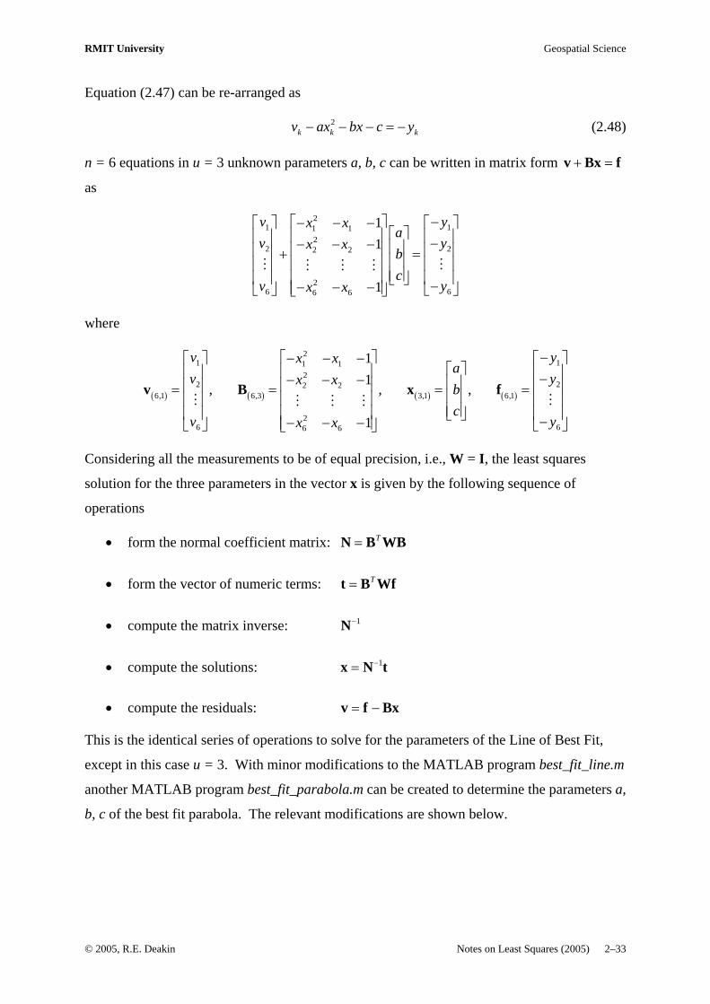
n = 6 equations in u = 3 unknown parameters a, b, c can be written in matrix form
as
+ =v Bx f
21 11 1
22 22 2
26 66 6
11
1
v yx xa
v yx xbc
v yx x
−⎡ ⎤− − −⎡ ⎤ ⎡ ⎤⎡ ⎤⎢ ⎥⎢ ⎥ ⎢ ⎥−− − − ⎢ ⎥⎢ ⎥⎢ ⎥ ⎢ ⎥+ =⎢ ⎥⎢ ⎥⎢ ⎥ ⎢ ⎥⎢ ⎥⎢ ⎥⎢ ⎥ ⎢ ⎥⎣ ⎦ −− − −⎢ ⎥⎣ ⎦ ⎣ ⎦⎣ ⎦
where
( ) ( ) ( ) ( )
21 11 1
22 22 2
6,1 6,3 3,1 6,1
26 66 6
11
, , ,
1
v yx xa
v yx xbc
v yx x
−⎡ ⎤− − −⎡ ⎤ ⎡ ⎤⎡ ⎤⎢ ⎥⎢ ⎥ ⎢ ⎥−− − − ⎢ ⎥⎢ ⎥⎢ ⎥ ⎢ ⎥= = = =⎢ ⎥⎢ ⎥⎢ ⎥ ⎢ ⎥⎢ ⎥⎢ ⎥⎢ ⎥ ⎢ ⎥⎣ ⎦ −− − −⎢ ⎥⎣ ⎦ ⎣ ⎦⎣ ⎦
v B x f
Considering all the measurements to be of equal precision, i.e., W = I, the least squares
solution for the three parameters in the vector x is given by the following sequence of
operations
• form the normal coefficient matrix: T=N B WB
• form the vector of numeric terms: T=t B Wf
• compute the matrix inverse: 1−N
• compute the solutions: 1−=x N t
• compute the residuals: = −v f Bx
This is the identical series of operations to solve for the parameters of the Line of Best Fit,
except in this case u = 3. With minor modifications to the MATLAB program best_fit_line.m
another MATLAB program best_fit_parabola.m can be created to determine the parameters a,
b, c of the best fit parabola. The relevant modifications are shown below.
© 2005, R.E. Deakin Notes on Least Squares (2005) 2–33

RMIT University Geospatial Science
MATLAB program best_fit_parabola
Making the following changes to the MATLAB program best_fit_line, a new program best_fit_parabola can be created. Changes to function name and help instructions function best_fit_parabola % % BEST_FIT_PARABOLA reads an ASCII textfile containing coordinate pairs (x,y) % and weights (w) associated with each pair and computes the parameters % a, b and c of a best fit parabola y = a(x*x) + bx + c using the least % squares principle. Results are written to a textfile having the same % path and name as the data file but with the extension ".out"
Changes to function remarks in documentation section % Remarks: % This function reads numeric data from a textfile containing coordinate % pairs (x,y) and weights (w) associated with each pair and computes the % parameters a, b, and c of a best fit parabola y = a(x*x) + bx + c using % the least squares principle. Results are written to a textfile having % the same path and name as the data file but with the extension ".out"
Changes to formation of coefficient matrix B % form the coefficient matrix B of the observation equations B = zeros(n,u); for k = 1:n B(k,1) = -(x_coord(k)^2); B(k,2) = -x_coord(k); B(k,3) = -1; end
Changes to data plotting section %------------------------------------------ % plot data points and Parabola of best fit %------------------------------------------ % copy solutions from vector x a = x(1,1); b = x(2,1); c = x(3,1); % find minimum and maximum x coordinates xmin = min(x_coord); xmax = max(x_coord); % create a vector of x coordinates at intervals of 0.1 % between min and max coordinates x = xmin:0.1:xmax; % calculate y coordinates of Parabola of Best Fit y = a*(x.*x) + b*x + c;
© 2005, R.E. Deakin Notes on Least Squares (2005) 2–34

RMIT University Geospatial Science
MATLAB program best_fit_parabola
Using the data from Figure 2.2 a data file c:\Temp\parabola_data.dat was created % data file for function "best_fit_parabola.m" % x y w 100.0 63.48 1 150.0 46.20 1 200.0 36.62 1 250.0 38.96 1 300.0 47.42 1 350.0 57.72 1
Running the program from the MATLAB command window generated the following output file c:\Temp\parabola_data.out and a plot of the Least Squares Parabola of best Fit Parabola of Best Fit Least Squares Solution Input Data x(k) y(k) weight w(k) 100.0000 63.4800 1.0000 150.0000 46.2000 1.0000 200.0000 36.6200 1.0000 250.0000 38.9600 1.0000 300.0000 47.4200 1.0000 350.0000 57.7200 1.0000 Coefficient matrix B of observation equations v + Bx = f -10000.0000 -100.0000 -1.0000 -22500.0000 -150.0000 -1.0000 -40000.0000 -200.0000 -1.0000 -62500.0000 -250.0000 -1.0000 -90000.0000 -300.0000 -1.0000 -122500.0000 -350.0000 -1.0000 Vector of numeric terms f of observation equations v + Bx = f -63.4800 -46.2000 -36.6200 -38.9600 -47.4200 -57.7200 Coefficient matrix N of Normal equations Nx = t 29218750000.0000 97875000.0000 347500.0000 97875000.0000 347500.0000 1350.0000 347500.0000 1350.0000 6.0000 Vector of numeric terms t of Normal equations Nx = t 16912600.0000 64770.0000 290.4000 Inverse of Normal equation coefficient matrix 4.2857e-009 -1.9286e-006 1.8571e-004 -1.9286e-006 8.9071e-004 -8.8714e-002 1.8571e-004 -8.8714e-002 9.3714e+000 Vector of solutions x 0.001500 -0.688221 116.350000
© 2005, R.E. Deakin Notes on Least Squares (2005) 2–35

RMIT University Geospatial Science
MATLAB program best_fit_parabola
Vector of residuals v -0.948 0.676 2.103 -0.889 -2.498 1.555
1 00 150 2 00 250 300 3 5035
40
45
50
55
60
65Least Squ ares Parabo la of Best Fit
X c oord inate
Y c
oord
inat
e
Figure 2.4 Least Squares Parabola of Best Fit
2.7.2. Least Squares Best Fit Ellipse
In November 1994, a survey was undertaken by staff of the Department of Geospatial Science
at the Melbourne Cricket Ground (MCG) to determine the dimensions of the playing surface.
This survey was to decide which of two sets of dimensions was correct, those of the
Melbourne Cricket Club (MCC) or those of the Australian Football League (AFL). The MCC
curator Tony Ware and the AFL statistician Col Hutchison both measured the length of the
ground (Tony Ware with a 100-metre nylon tape and Col Hutchison with a measuring wheel)
and compared their distances with the "true" distance determined by Electronic Distance
Measurement (EDM) with a Topcon 3B Total Station. Their measurements were both
reasonably close to the EDM distance and it turned out that the "official" AFL dimensions
© 2005, R.E. Deakin Notes on Least Squares (2005) 2–36

RMIT University Geospatial Science
were incorrect. After this "measure-off", observations (bearings and distances) were made to
seventeen points around the edge of the playing surface to determine the Least Squares
Ellipse of Best Fit and to see if the major axis of this ellipse was the actual line between the
goals at either end. The Total Station was set-up close to the goal-to-goal axis and 20-25
metres from the centre of the ground. An arbitrary X,Y coordinate system was used with the
origin at the Total Station and the positive X-axis in the direction of the Brunton Avenue end
of the Great Southern Stand (approximately west). The table of coordinates is given below;
point numbers 1 to 6 were not points on the edge of the ground.
Point No. X-coordinate Y-coordinate
7 -54.58 17.11 8 -45.47 36.56 9 -28.40 53.22 10 -2.02 63.72 11 28.12 63.44 12 57.49 52.55 13 80.85 34.20 14 98.08 9.14 15 105.69 -17.30 16 103.83 -46.96 17 88.42 -71.50 18 61.26 -86.84 19 26.47 -91.07 20 -6.59 -81.37 21 -34.55 -59.24 22 -51.51 -29.28 23 -56.30 -2.31
Table 2.4 Arbitrary coordinates of points around the perimeter of the playing surface of the MCG (date of survey November 1994)
To develop an observation equation for the Least Squares Ellipse of Best Fit and to determine
the lengths and directions of the axes of the ellipse the following derivation of the general
equation of an ellipse is necessary.
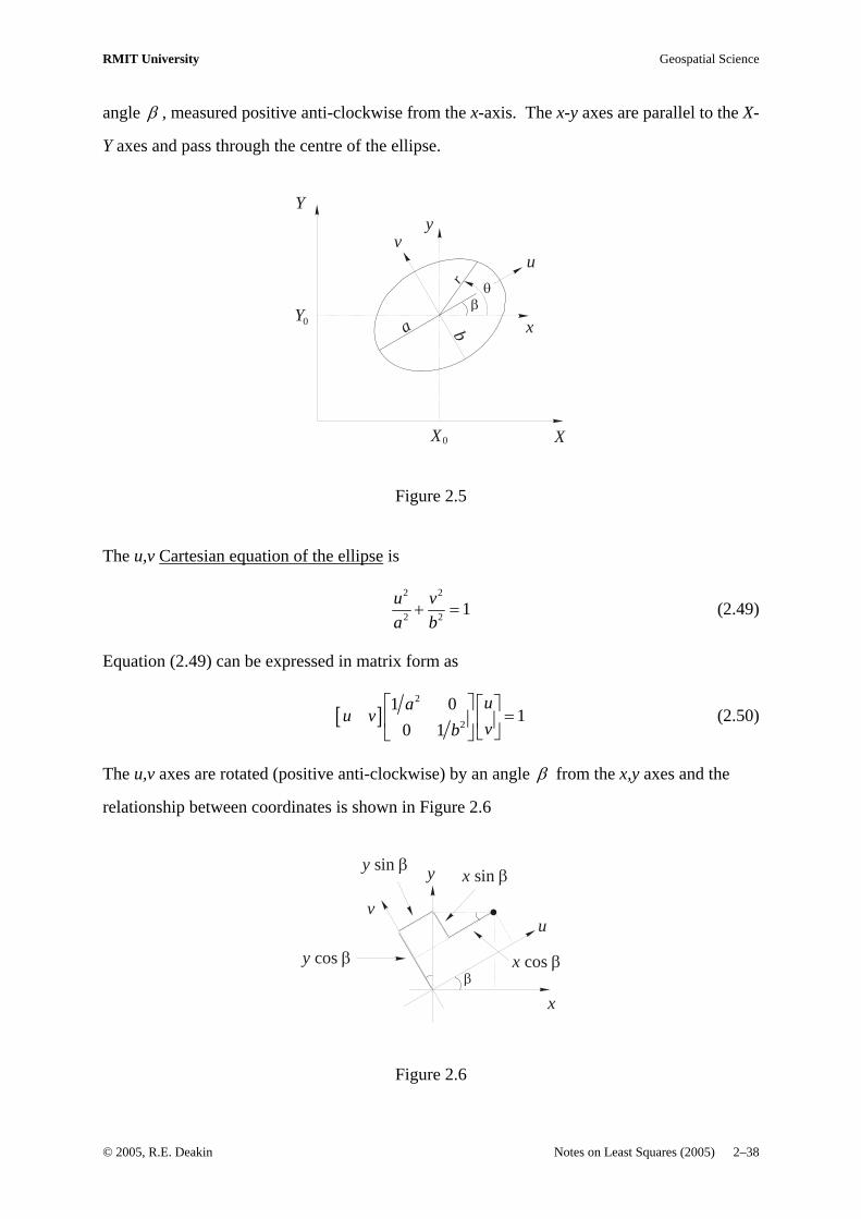
Figure 2.5 shows an ellipse whose axes are aligned with the u-v axes. The semi-axes lengths
are a and b ( ) , the centre of the ellipse is at a b> 0 0,X Y and the ellipse axes are rotated by an
© 2005, R.E. Deakin Notes on Least Squares (2005) 2–37
RMIT University Geospatial Science
angle β , measured positive anti-clockwise from the x-axis. The x-y axes are parallel to the X-
Y axes and pass through the centre of the ellipse.
y
xa b
Y
X
0
0
Y
X
β
r θ
uv
Figure 2.5
The u,v Cartesian equation of the ellipse is
2 2
2 2 1u va b
+ = (2.49)
Equation (2.49) can be expressed in matrix form as
[ ]2
2
1 01
0 1ua
u vvb
⎡ ⎤ ⎡ ⎤=⎢ ⎥ ⎢ ⎥
⎣ ⎦⎣ ⎦ (2.50)
The u,v axes are rotated (positive anti-clockwise) by an angle β from the x,y axes and the
relationship between coordinates is shown in Figure 2.6
y
xβ
uv •
y cos β
x sin β
x cos β
y sin β
Figure 2.6
© 2005, R.E. Deakin Notes on Least Squares (2005) 2–38

RMIT University Geospatial Science
Inspection of Figure 2.6 shows
cos sinsin cos
u x yv x y
β ββ β
= += − +
(2.51)
Replacing cos β and sin β with the letters c and s the coordinate relationships can be
represented as a matrix equation
c ss c
u xv y
⎡ ⎤ ⎡ ⎤ ⎡ ⎤=⎢ ⎥ ⎢ ⎥ ⎢ ⎥−⎣ ⎦ ⎣ ⎦ ⎣ ⎦
(2.52)
Transposing this equation (remembering the reversal rule with the transpose of matrix
products) gives
[ ] [ ] c ss c
u v x y−⎡ ⎤
= ⎢ ⎥⎣ ⎦
(2.53)
Substituting (2.52) and (2.53) into (2.50) and multiplying the matrices gives
[ ]
[ ]
2
2
2 2
2 2 2 2
2 2
2 2 2 2
c s c s1 01
s c s c0 1
c s cs cs
1cs cs s c
xax y
yb
a b a b xx y
ya b a b
− ⎡ ⎤⎡ ⎤ ⎡ ⎤ ⎡ ⎤=⎢ ⎥⎢ ⎥ ⎢ ⎥ ⎢ ⎥−⎣ ⎦ ⎣ ⎦ ⎣ ⎦⎣ ⎦
⎡ ⎤⎛ ⎞ ⎛ ⎞+ −⎢ ⎥⎜ ⎟⎜ ⎟⎝ ⎠ ⎡ ⎤⎝ ⎠⎢ ⎥ =⎢ ⎥⎢ ⎥⎛ ⎞ ⎣ ⎦⎛ ⎞⎢ ⎥− +⎜ ⎟ ⎜ ⎟
⎝ ⎠⎢ ⎥⎝ ⎠⎣ ⎦
Replacing the elements of the square matrix with the symbols A, B and H, noting that the top-
right and lower-left elements are the same, this equation may be written in a general form as
[ ] 1A H x
x yH B y
⎡ ⎤ ⎡ ⎤=⎢ ⎥ ⎢ ⎥
⎣ ⎦ ⎣ ⎦
or 2 2Ax Hxy By2 1+ + = (2.54)
Equation (2.54) is the equation of an ellipse centred at the coordinate origin but with axes
rotated from the x,y axes. The semi axes lengths a and b, and the rotation angle β can be
determined from (2.54) by the following method.
Letting cosx r θ= and siny r θ= in equation (2.54) gives the polar equation of the ellipse
© 2005, R.E. Deakin Notes on Least Squares (2005) 2–39

RMIT University Geospatial Science
22
1cos 2 cos sin sinA H Br
θ θ θ θ+ + 2 = (2.55)
r is the radial distance from the centre of the ellipse and θ is the angle measured positive
anti-clockwise from the x-axis. Equation (2.55) has maximum and minimum values defining
the lengths and directions of the axes of the ellipse. To determine these values from (2.55),
consider the following
Let 2 22
2 2
1 cos 2 cos sin sin
cos sin 2 sin
f A H Br
A H B
θ θ θ
θ θ θ
= = + +
= + +
θ
and aim to find the optimal (maximum and minimum) values of f and the values of θ when
these occur by investigating the first and second derivatives f ′ and f ′′ respectively, i.e.,
max 0 and 0
is when min 0 and 0
f ff
f f′ ′′= <⎧ ⎫ ⎧
⎨ ⎬ ⎨ ′ ′′= >⎩ ⎭ ⎩
⎫⎬⎭
2
where ( )
( )sin 2 2 cos2
2 cos2 4 sin
f B A H
f B A H
θ θ
θ θ
′ = − +
′′ = − − (2.56)
Now the maximum or minimum value of f occurs when 0f ′ = and from the first member of
(2.56) the value of θ is given by
2tan 2 HA B
θ =−
(2.57)
But this value of θ could relate to either a maximum or a minimum value of f. So from the
second member of equations (2.56) with a value of 2θ from equation (2.57) this ambiguity
can be resolved by determining the sign of the second derivative f ′′ giving
max
min
0 when
0f ff f
′′ <⎧ ⎫ ⎧ ⎫⎨ ⎬ ⎨ ′′ >⎩ ⎭⎩ ⎭
⎬
In the polar equation of the ellipse given by equation (2.55) maxf coincides with and minr minf
coincides with so the angle maxr β (measured positive anti-clockwise) from the x-axis to the
major axis of the ellipse (see Figure 2.5) is found from
max1
min 2
0 when and
0r fr f
β θβ θ π
′′ => ⎧ ⎫⎧ ⎫ ⎧ ⎫⎨ ⎬ ⎨ ⎬ ⎨′′ = −<⎩ ⎭⎩ ⎭ ⎩ ⎭
⎬ (2.58)
© 2005, R.E. Deakin Notes on Least Squares (2005) 2–40

RMIT University Geospatial Science
These results can be verified by considering the definitions of A, B and H used in the
derivation of the polar equation of the ellipse, i.e.,
2 2 2 2
2 2 2 2 2 2
cos sin sin cos cos sin cos sin, ,A B Ha b a b a b
β β β β β β β= + = + = −
β
and 2 2 2 2
1 1 1 1cos2 , 2 sin 2A B Ha b a b
β β⎛ ⎞ ⎛ ⎞− = − = −⎜ ⎟ ⎜ ⎟⎝ ⎠ ⎝ ⎠
giving 2tan 2 HA B
β =−
Noting that the values of θ coinciding with the maximum or minimum values of the function
f are found from equation (2.57) then 2tan 2 tan 2HA B
β θ= =−
or
tan 2 tan 2θ β=
whereupon
122 2 or where is an integern n nθ β π θ β π= + = +
Also, from the second member of equations (2.56)
( )2 cos2 4 sinf B A H 2θ θ′′ = − −
Now, for 0n =
θ β= , 2 2
1 12fa bθ β=
⎛′′ = − −⎜⎝ ⎠
⎞⎟ and since a b , > 0f
θ β=′′ >
So θ β= makes f minimum and so r is maximum and
( )
2 2min
22 2
2 2
cos 2 sin cos sin
cos sin 1
f A H B
a a
β β β
β β
= + +
+= =
β
So maxr a=
When 1n =
12θ β π= + , sin 2 sin 2θ β= − , cos2 cos2θ β= − and so
12
2 2
1 12fa bθ β π= +
⎛′′ = −⎜⎝ ⎠
⎞⎟ and since a b , > 1
20f
θ β π= +′′ <
So 12θ β π= + makes f maximum and so r is minimum and
© 2005, R.E. Deakin Notes on Least Squares (2005) 2–41

RMIT University Geospatial Science
( )22 2
max 2 2
sin cos 1fb b
β β+= =
So minr b=
When 2n =
θ β π= + , sin 2 cos2θ β= , cos2 cos2θ β= and 0fθ β π= +
′′ >
So 12θ β π= + makes min 2
1fa
= and maxr a=
When 3n =
32θ β π= + , sin 2 cos2θ β= − , cos2 cos2θ β= − and 3
20f
θ β π= +′′ <
So 32θ β π= + makes max 2
1fb
= and minr b=
All other even values of n give the same result as 2n = and all other odd values of n give the
same result as 1n =
Now consider Figure 2.5 and the general Cartesian equation of the ellipse, re-stated again as
(2.59) 2 22aX hXY bY dX eY+ + + + 1=
where the translated x,y coordinate system is related to the X,Y system by
0X x X= + and 0Y y Y= +
Substituting these relationships into (2.59) gives
( ) ( ) ( ) ( ) ( ) ( )2 20 0 0 0 02 1a x X h x X y Y b y Y d x X e y Y+ + + + + + + + + + =0
Expanding and gathering terms gives
( )( )
2 20 0
0 0
2 20 0 0 0 0 0
2 2 2
2 2
2 1
ax hxy by aX hY d x
aY hX e y
aX hX Y bY dX eY
+ + + + +
+ + +
+ + + + + =
2
Inspection of the left-hand-side of this equation reveals three parts:
(i) is the left-hand-side of the equation of an ellipse, similar in form
to equation
2 2ax hxy by+ +
(2.54) ,
(ii) coefficient terms of x and y; ( )0 02 2aX hY d+ + and ( )0 02 2aY hX e+ + ,
© 2005, R.E. Deakin Notes on Least Squares (2005) 2–42

RMIT University Geospatial Science
(iii) a constant term 2 20 0 0 0 02aX hX Y bY dX eY+ + + + 0
2
Now when the coefficients of x and y are zero the ellipse will be centred at the origin of the
x,y axes with an equation of the form
2 2ax hxy by c+ + = (2.60)
where ( )2 20 0 0 0 01 2c aX hX Y bY dX eY= − + + + + 0
00
(2.61)
and 0 0
0 0
2 22 2aX hY dhX bY e
+ + =+ + =
(2.62)
Equations (2.62) can be written in matrix form and solved (using the inverse of a 2,2 matrix)
to give 0X and 0Y
0
0
02
0
2 22 2
12 2
Xd a hYe h b
X b h dY h a eab h
− − ⎡ ⎤⎡ ⎤ ⎡ ⎤= ⎢ ⎥⎢ ⎥ ⎢ ⎥− −⎣ ⎦ ⎣ ⎦ ⎣ ⎦
−⎡ ⎤ ⎡ ⎤ ⎡ ⎤=⎢ ⎥ ⎢ ⎥ ⎢ ⎥−− ⎣ ⎦ ⎣ ⎦⎣ ⎦
giving ( )0 22eh bdXab h
−=
− and ( )0 22
dh aeYab h
−=
− (2.63)
Dividing both sides of (2.60) by c gives
2 2Ax Hxy By2 1+ + = (2.64)
where , ,a hA H Bc c
bc
= = =
Equation (2.64), identical to equation (2.54), is the equation of an ellipse centred at the x,y
coordinate origin whose axes are rotated from the x,y axes by an angle β . The rotation angle
β and semi-axes lengths a and b of the ellipse can be determined using the method set out
above and equations (2.58), (2.57), (2.56) and (2.55). Thus, we can see from the development
that the general Cartesian equation of an ellipse is given by
(2.65) 2 22aX hXY bY dX eY+ + + + 1=
Note that the coefficients a and b in this equation are not the semi-axes lengths of the ellipse.
© 2005, R.E. Deakin Notes on Least Squares (2005) 2–43
RMIT University Geospatial Science
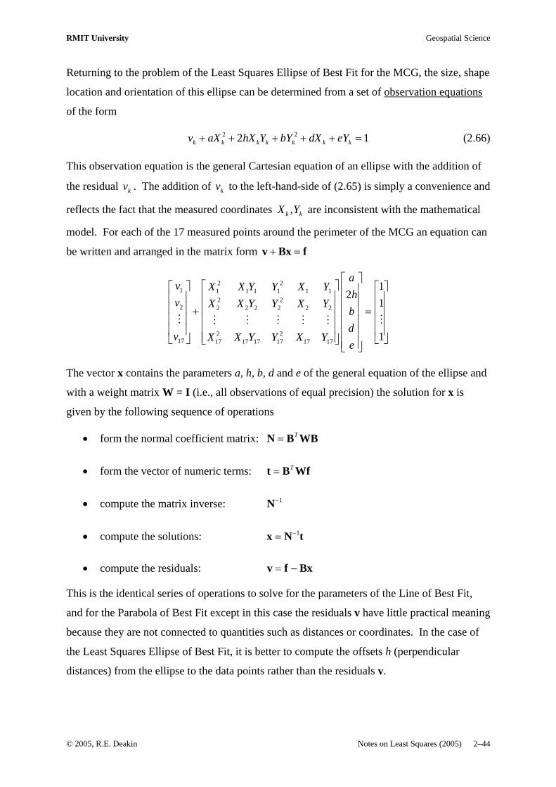
Returning to the problem of the Least Squares Ellipse of Best Fit for the MCG, the size, shape
location and orientation of this ellipse can be determined from a set of observation equations
of the form
(2.66) 2 22k k k k k k kv aX hX Y bY dX eY+ + + + + = 1
This observation equation is the general Cartesian equation of an ellipse with the addition of
the residual . The addition of to the left-hand-side of kv kv (2.65) is simply a convenience and
reflects the fact that the measured coordinates ,k kX Y are inconsistent with the mathematical
model. For each of the 17 measured points around the perimeter of the MCG an equation can
be written and arranged in the matrix form + =v Bx f
2 21 1 1 1 1 1 1
2 22 2 2 2 2 2 2
2 217 17 17 17 17 17 17
12
1
1
av X X Y Y X Y
hv X X Y Y X Y
bd
v X X Y Y X Ye
⎡ ⎤⎡ ⎤⎡ ⎤ ⎡ ⎤⎢ ⎥⎢ ⎥⎢ ⎥ ⎢ ⎥⎢ ⎥⎢ ⎥⎢ ⎥ ⎢ ⎥+ =⎢ ⎥⎢ ⎥⎢ ⎥ ⎢ ⎥⎢ ⎥⎢ ⎥⎢ ⎥ ⎢ ⎥⎢ ⎥⎢ ⎥ ⎣ ⎦⎣ ⎦ ⎣ ⎦ ⎢ ⎥⎣ ⎦
The vector x contains the parameters a, h, b, d and e of the general equation of the ellipse and
with a weight matrix W = I (i.e., all observations of equal precision) the solution for x is
given by the following sequence of operations
• form the normal coefficient matrix: T=N B WB
• form the vector of numeric terms: T=t B Wf
• compute the matrix inverse: 1−N
• compute the solutions: 1−=x N t
• compute the residuals: = −v f Bx
This is the identical series of operations to solve for the parameters of the Line of Best Fit,
and for the Parabola of Best Fit except in this case the residuals v have little practical meaning
because they are not connected to quantities such as distances or coordinates. In the case of
the Least Squares Ellipse of Best Fit, it is better to compute the offsets h (perpendicular
distances) from the ellipse to the data points rather than the residuals v.
© 2005, R.E. Deakin Notes on Least Squares (2005) 2–44

RMIT University Geospatial Science
To compute offsets h the following preliminary sequence of operations is required:
(i) compute the parameters a, h, b, d and e using the Least Squares process set out
above.
(ii) compute the coordinates of the origin 0 0,X Y and the constant c using equations
(2.63) and (2.61).
(iii) compute coefficients A, H and B of the ellipse given by (2.64) which can then be
used to compute the rotation angle β and the semi-axes lengths a and b from
equations (2.55) to (2.58) and.
(iv) compute the u,v coordinates of the data points using equations (2.51).
Now, having the u,v coordinates, the offsets h can be computed. Consider the sectional view
of a quadrant of an ellipse in Figure 2.7. The u,v axes are in the direction of the major and
minor axes respectively (a and b are the semi-axes lengths) and P is a point related to the
ellipse by the normal, which makes an angle φ with the major axis, and the distance h = QP
along the normal. The u,v coordinates of P are the distances LP and MP respectively. From
the geometry of an ellipse, the normal intersects the minor axis at H and the distance QH ν=
(where ν is the Greek symbol nu) and the distances DH and OH are 2eν and 2 sineν φ
respectively. e is the eccentricity of the ellipse and the eccentricity and flattening f of an
ellipse are related to the semi-axes a and b.
© 2005, R.E. Deakin Notes on Least Squares (2005) 2–45
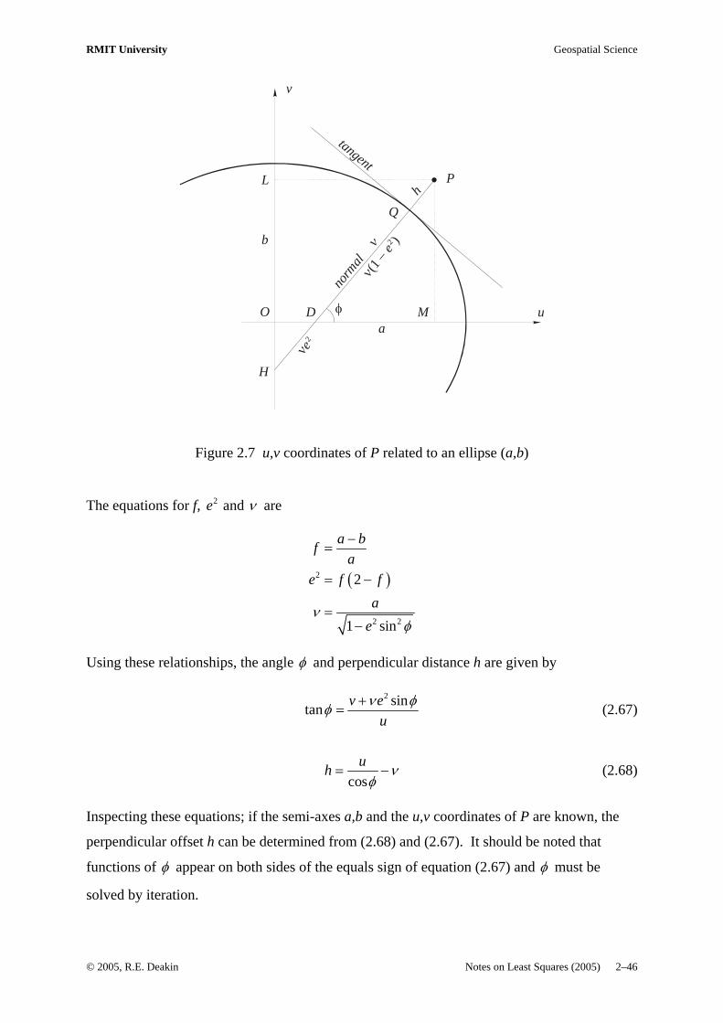
RMIT University Geospatial Science
tangent
norm
alH
O
•
φ
P
Q
D u
v
h
b
a
νe2
ν(1 −
e )2ν
L
M
Figure 2.7 u,v coordinates of P related to an ellipse (a,b)
The equations for f, 2 and e ν are
( )2
2 2
2
1 sin
a bfa
e f fa
eν
φ
−=
= −
=−
Using these relationships, the angle φ and perpendicular distance h are given by
2 sintan v e
uν φφ +
= (2.67)
cos
uh νφ
= − (2.68)
Inspecting these equations; if the semi-axes a,b and the u,v coordinates of P are known, the
perpendicular offset h can be determined from (2.68) and (2.67). It should be noted that
functions of φ appear on both sides of the equals sign of equation (2.67) and φ must be
solved by iteration.
© 2005, R.E. Deakin Notes on Least Squares (2005) 2–46

RMIT University Geospatial Science
To determine the Least Square Best Fit Ellipse for the playing surface of the MCG a
MATLAB program best_fit_ellipse.m operating in the same way as the MATLAB programs
best_fit_line and best_fit_parabola with a data file (in this example: MCG_ellipse_data.dat)
Data file c:\Temp\MCG_ellipse_data.dat % Data file for MCG Survey, November 1994 % Coordinates of 17 boundary points (edge of concrete) % % point X Y weight 7 -54.58 17.11 1 8 -45.47 36.56 1 9 -28.40 53.22 1 10 -2.02 63.72 1 11 28.12 63.44 1 12 57.49 52.55 1 13 80.85 34.20 1 14 98.08 9.14 1 15 105.69 -17.30 1 16 103.83 -46.96 1 17 88.42 -71.50 1 18 61.26 -86.84 1 19 26.47 -91.07 1 20 -6.59 -81.37 1 21 -34.55 -59.24 1 22 -51.51 -29.28 1 23 -56.30 -2.31 1
gives the following results (contained in an output file having the same name and path as the
data file but with the extension .dat) and plot on the screen.
Output file c:\Temp\MCG_ellipse_data.out Ellipse of Best Fit Least Squares Solution Input Data point x(k) y(k) weight w(k) 7 -54.5800 17.1100 1.0000 8 -45.4700 36.5600 1.0000 9 -28.4000 53.2200 1.0000 10 -2.0200 63.7200 1.0000 11 28.1200 63.4400 1.0000 12 57.4900 52.5500 1.0000 13 80.8500 34.2000 1.0000 14 98.0800 9.1400 1.0000 15 105.6900 -17.3000 1.0000 16 103.8300 -46.9600 1.0000 17 88.4200 -71.5000 1.0000 18 61.2600 -86.8400 1.0000 19 26.4700 -91.0700 1.0000 20 -6.5900 -81.3700 1.0000 21 -34.5500 -59.2400 1.0000 22 -51.5100 -29.2800 1.0000 23 -56.3000 -2.3100 1.0000
© 2005, R.E. Deakin Notes on Least Squares (2005) 2–47

RMIT University Geospatial Science
General Equation of Ellipse with X,Y origin not at centre of ellipse aXX + 2hXY + bYY + dX + eY = 1 a = 1.720717e-004 h = 2.690541e-005 b = 1.865607e-004 d = -7.743828e-005 e = 3.729881e-005 Equation of Ellipse with x,y origin at centre of ellipse Axx + 2Hxy + Byy = 1 A = 1.535544e-004 H = 2.401002e-005 B = 1.664842e-004 Ellipse parameters semi-major axis a = 86.017 semi-minor axis b = 73.544 Bearing of major axis beta(degrees) = -37.465030 beta(DMS) = -37 27 54.11 Brg(degrees) = 127.465030 Brg(DMS) = 127 27 54.11 Coordinates of centre of ellipse X(centre) = 24.620 Y(centre) = -13.547 Data and offsets to ellipse of best fit pt offset X Y x y u v 7 0.129 -54.580 17.110 -79.200 30.657 -81.511 -23.842 8 0.159 -45.470 36.560 -70.090 50.107 -86.111 -2.863 9 0.162 -28.400 53.220 -53.020 66.767 -82.696 20.744 10 0.164 -2.020 63.720 -26.640 77.267 -68.145 45.124 11 0.060 28.120 63.440 3.500 76.987 -44.051 63.236 12 -0.090 57.490 52.550 32.870 66.097 -14.116 72.457 13 -0.223 80.850 34.200 56.230 47.747 15.588 72.101 14 -0.216 98.080 9.140 73.460 22.687 44.507 62.691 15 -0.123 105.690 -17.300 81.070 -3.753 66.630 46.334 16 0.936 103.830 -46.960 79.210 -33.413 83.195 21.661 17 0.284 88.420 -71.500 63.800 -57.953 85.891 -7.191 18 -1.181 61.260 -86.840 36.640 -73.293 73.664 -35.887 19 -0.224 26.470 -91.070 1.850 -77.523 48.624 -60.407 20 0.627 -6.590 -81.370 -31.210 -67.823 16.483 -72.817 21 0.554 -34.550 -59.240 -59.170 -45.693 -19.171 -72.259 22 -0.438 -51.510 -29.280 -76.130 -15.733 -50.856 -58.796 23 -0.703 -56.300 -2.310 -80.920 11.237 -71.063 -40.303
© 2005, R.E. Deakin Notes on Least Squares (2005) 2–48

RMIT University Geospatial Science
-60 -40 -20 0 20 40 60 80 100 120
-80
-60
-40
-20
0
20
40
60
7
8
910 11
12
13
14
15
16
17
181920
21
22
23
Least Squares Ellipse of Best Fit
X coordinate
Y co
ordi
nate
Brunton Avegoals
Punt Rdgoals
MCG
Figure 2.8 Plot of Least Squares Best Fit Ellipse and data points for the MCG
The MATLAB program best_fit_ellipse.m calls two other MATLAB functions ellipse.m (a
function to compute the coordinates of points on an ellipse) and DMS.m (a function to convert
decimal degree to degrees, minutes and seconds). A copy of these programs is shown below.
© 2005, R.E. Deakin Notes on Least Squares (2005) 2–49

RMIT University Geospatial Science
MATLAB program best_fit_ellipse
function best_fit_ellipse % % BEST_FIT_ELLIPSE reads an ASCII textfile containing point numbers of % coordinate pairs (X,Y) and weights (W) associated with each pair and % computes the cordinates of the origin, the lengths of the axes and % the rotation angle of the Best Fit Ellipse using the least squares % principle. Results are written to a textfile having the same path % and name as the data file but with the extension ".out" %============================================================================ % Function: best_fit_ellipse % % Author: % Rod Deakin, % School of Mathematical and Geospatial Sciences, RMIT University, % GPO Box 2476V, MELBOURNE VIC 3001 % AUSTRALIA % email: [email protected] % % Date: % Version 1.0 22 March 2003 % Version 1.1 10 May 2003 % Version 1.2 9 November 2005 % % Functions Required: % [X,Y] = ellipse(a,b,theta) % [D,M,S] = DMS(DecDeg) % % Remarks: % The general equation of an ellipse is % aXX + 2hXY + bYY + dX + eY = 1 % This function computes the parameters a,h,b,d,e of a Least Squares Best Fit % Ellipse given a set of X,Y coordinate pairs and weights (w) associated with % each pair. The centre of the best fit ellipse is at Xo = (eh-db)/(2ab-2hh) % and Yo = (dh-ea)/(2ab-2hh). % A constant c = 1 - (aXoXo + 2hXoYo + bYoYo + dXo + eYo) is divided into a, % h and b giving A = a/c, H = h/c and B = b/c which are the parameters of an % ellipse Axx +2Hxy + Byy = 1. The major axis of this ellipse is rotated % from the coordinate axes by an angle beta which can be determined from the % polar equation of an ellipse % A*cos_squared(theta) + 2H*cos(theta)*sin(theta) + B*sin_squared(theta) = 1/r_squared % The maximum and minimum values of this function occur for theta given by % tan(2*theta) = 2H/(A-B) and the angle beta is determined by evaluating % the sign of the second derivative of the polar equation. This angle is % substituted into the polar equation to determine the length of the semi-major % axis length a. Beta - 90 degrees will give the length of the semi-minor % axis length b % Note that the semi-axes lengths a,b are not the same as the parameters % a and b in the general equation of the ellipse. % Results are written to a textfile having the same path and name as the % data file but with the extension ".out" % % References: % Notes on Least Squares (2005), Geospatial Science, RMIT % University, 2005 %
© 2005, R.E. Deakin Notes on Least Squares (2005) 2–50

RMIT University Geospatial Science
MATLAB program best_fit_ellipse
% Arrays: % B - coeff matrix of observation equation v + Bx = f % f - vector of numeric terms % N - coefficient matrix of Normal equations Nx = t % Ninv - inverse of N % p - vector of perpendicular distances from ellipse to points % point - vector of point numbers % t - vector of numeric terms of Normal equations Nx = t % u,v - vectors of u,v coords of ellipse % W - weight matrix % weight - vector of weights % x - vector of solutions % x,y - vectors of x,y coords of ellipse % x_coord - vector of X coordinates % y_coord - vector of Y coordinates % xpt,ypt - vectors of coords for point number locations on plot % Xpt,Ypt - vectors Xpt = xpt + Xc, Ypt = ypt + Yc % % % Variables: % A,B,H - parameters of ellipse Axx + 2Hxy + Byy = 1 % a,h,b, - parameters of ellipse aXX + 2hXY + bYY + dX + eY = 1 % d,e % a1,b1 - semi-major and semi-minor axes of ellipse % beta - angle between x-axis and major axis of ellipse (degrees) % brg - bearing of major axis (u-axis) of ellipse (degrees) % c - constant of translated ellipse or cos(x) % d2r - degree to radian conversion factor = 180/pi = 57.29577951... % e2 - eccentricity squared % flat - flattening of ellipse % f_dd - second derivative of the function "f" where f is the polar % equation of an ellipse % lat - latitude (radians) of point related to an ellipse % n - number of equations % new_lat - new latitude in iteration % nu - radius of curvature in prime meridian % pion2 - 90 degrees or pi/2 % u - number of unknowns % s - sin(x) % s1,s2 - sin(lat) and sin_squared(lat) % scale - scale factor to reduce size of numbers in normal equations % theta - angle for which polar equation of ellipse gives max/min % values % two_theta - 2*theta % Xc,Yc - coords of centre of ellipse X = x + Xc, Y = y + Yc % X0,Y0 - scaled coords of centre of ellipse % %============================================================================ % % Set program constants d2r = 180/pi; pion2 = pi/2; scale = 100;
© 2005, R.E. Deakin Notes on Least Squares (2005) 2–51

RMIT University Geospatial Science
MATLAB program best_fit_ellipse
%------------------------------------------------------------------------- % 1. Call the User Interface (UI) to choose the input data file name % 2. Concatenate strings to give the path and file name of the input file % 3. Strip off the extension from the file name to give the rootName % 4. Add extension ".out" to rootName to give the output filename % 5. Concatenate strings to give the path and file name of the output file %------------------------------------------------------------------------- filepath = strcat('c:\temp\','*.dat'); [infilename,inpathname] = uigetfile(filepath); infilepath = strcat(inpathname,infilename); rootName = strtok(infilename,'.'); outfilename = strcat(rootName,'.out'); outfilepath = strcat(inpathname,outfilename); %---------------------------------------------------------- % 1. Load the data into an array whose name is the rootName % 2. set fileTemp = rootName % 3. Copy columns of data into individual arrays %---------------------------------------------------------- load(infilepath); fileTemp = eval(rootName); point = fileTemp(:,1); x_coord = fileTemp(:,2); y_coord = fileTemp(:,3); weight = fileTemp(:,4); % Determine the number of equations and set the number of unknowns n = length(point); u = 5; % Set the elements of the weight matrix W W = zeros(n,n); for k = 1:n W(k,k) = weight(k); end % Form the coefficient matrix B of the observation equations. % Note that the coordinates are scaled by a factor 1/100 to % reduce the size of equations. B = zeros(n,u); for k = 1:n B(k,1) = (x_coord(k)/scale)^2; B(k,2) = (x_coord(k)/scale)*(y_coord(k)/scale); B(k,3) = (y_coord(k)/scale)^2; B(k,4) = x_coord(k)/scale; B(k,5) = y_coord(k)/scale; end % Form the vector of numeric terms f f = ones(n,1); % Form the normal equation coefficient matrix N % and the vector of numeric terms t N = B'*W*B; t = B'*W*f; % Compute the inverse and solve the system Nx = t Ninv = inv(N); x = Ninv*t;
© 2005, R.E. Deakin Notes on Least Squares (2005) 2–52

RMIT University Geospatial Science
MATLAB program best_fit_ellipse
% Copy the results into the variables a,h,b,d,e a = x(1,1); h = x(2,1)/2; b = x(3,1); d = x(4,1); e = x(5,1); % Compute the coordinates of the centre of the ellipse X0 = (e*h - b*d)/(2*(a*b - h*h)); Y0 = (d*h - a*e)/(2*(a*b - h*h)); Xc = X0*scale; Yc = Y0*scale; % Compute the variables A,H,B and then the lengths % of the axes and the rotation angle beta c = 1-(a*X0*X0 + 2*h*X0*Y0 + b*Y0*Y0 + d*X0 + e*Y0); A = a/c; H = h/c; B = b/c; % compute the angle theta for max or min two_theta = atan2(2*H,(A-B)); % compute second derivative f_dd = 2*(B-A)*cos(two_theta) - 4*H*sin(two_theta); % test the second derivative to determine max or min theta = two_theta/2; if f_dd < 0 beta = theta - pion2; else beta = theta; end % compute semi-major axis length c = cos(beta); s = sin(beta); a1 = sqrt(1/(A*c*c + 2*H*c*s + B*s*s))*scale; % compute semi-minor axis length c = cos(beta+pion2); s = sin(beta+pion2); b1 = sqrt(1/(A*c*c + 2*H*c*s + B*s*s))*scale; % convert beta to degrees beta = beta*d2r; % Calculate bearing of major axis noting that the rotation angle % beta is considered positive anti-clockwise from the X-axis to % the major axis of the ellipse brg = 360+90-beta; if(brg>360) brg = brg-360; end %----------------------------------------------------------------------- % Compute perpendicular distances from points to the ellipse of best fit %----------------------------------------------------------------------- % Create a set of u,v coordinates by first reducing the X,Y coords % to x,y coordinates and then rotating these coordinates by the % rotation angle beta. The u-axis is the major axis of the ellipse. x = x_coord-Xc; y = y_coord-Yc; for k=1:n u(k,1) = x(k)*cos(beta/d2r) + y(k)*sin(beta/d2r); v(k,1) = -x(k)*sin(beta/d2r) + y(k)*cos(beta/d2r); end
© 2005, R.E. Deakin Notes on Least Squares (2005) 2–53
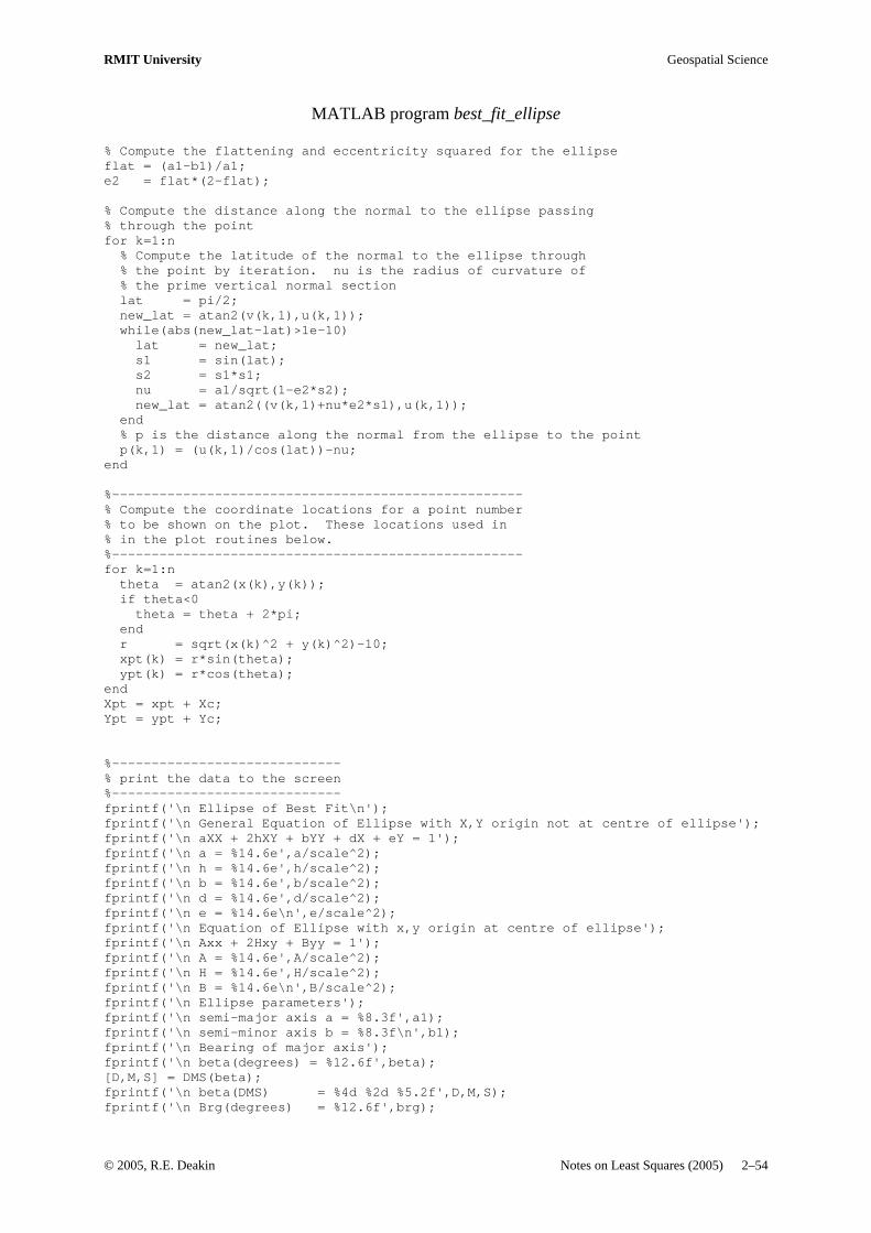
RMIT University Geospatial Science
MATLAB program best_fit_ellipse
% Compute the flattening and eccentricity squared for the ellipse flat = (a1-b1)/a1; e2 = flat*(2-flat); % Compute the distance along the normal to the ellipse passing % through the point for k=1:n % Compute the latitude of the normal to the ellipse through % the point by iteration. nu is the radius of curvature of % the prime vertical normal section lat = pi/2; new_lat = atan2(v(k,1),u(k,1)); while(abs(new_lat-lat)>1e-10) lat = new_lat; s1 = sin(lat); s2 = s1*s1; nu = a1/sqrt(1-e2*s2); new_lat = atan2((v(k,1)+nu*e2*s1),u(k,1)); end % p is the distance along the normal from the ellipse to the point p(k,1) = (u(k,1)/cos(lat))-nu; end %---------------------------------------------------- % Compute the coordinate locations for a point number % to be shown on the plot. These locations used in % in the plot routines below. %---------------------------------------------------- for k=1:n theta = atan2(x(k),y(k)); if theta<0 theta = theta + 2*pi; end r = sqrt(x(k)^2 + y(k)^2)-10; xpt(k) = r*sin(theta); ypt(k) = r*cos(theta); end Xpt = xpt + Xc; Ypt = ypt + Yc; %----------------------------- % print the data to the screen %----------------------------- fprintf('\n Ellipse of Best Fit\n'); fprintf('\n General Equation of Ellipse with X,Y origin not at centre of ellipse'); fprintf('\n aXX + 2hXY + bYY + dX + eY = 1'); fprintf('\n a = %14.6e',a/scale^2); fprintf('\n h = %14.6e',h/scale^2); fprintf('\n b = %14.6e',b/scale^2); fprintf('\n d = %14.6e',d/scale^2); fprintf('\n e = %14.6e\n',e/scale^2); fprintf('\n Equation of Ellipse with x,y origin at centre of ellipse'); fprintf('\n Axx + 2Hxy + Byy = 1'); fprintf('\n A = %14.6e',A/scale^2); fprintf('\n H = %14.6e',H/scale^2); fprintf('\n B = %14.6e\n',B/scale^2); fprintf('\n Ellipse parameters'); fprintf('\n semi-major axis a = %8.3f',a1); fprintf('\n semi-minor axis b = %8.3f\n',b1); fprintf('\n Bearing of major axis'); fprintf('\n beta(degrees) = %12.6f',beta); [D,M,S] = DMS(beta); fprintf('\n beta(DMS) = %4d %2d %5.2f',D,M,S); fprintf('\n Brg(degrees) = %12.6f',brg);
© 2005, R.E. Deakin Notes on Least Squares (2005) 2–54
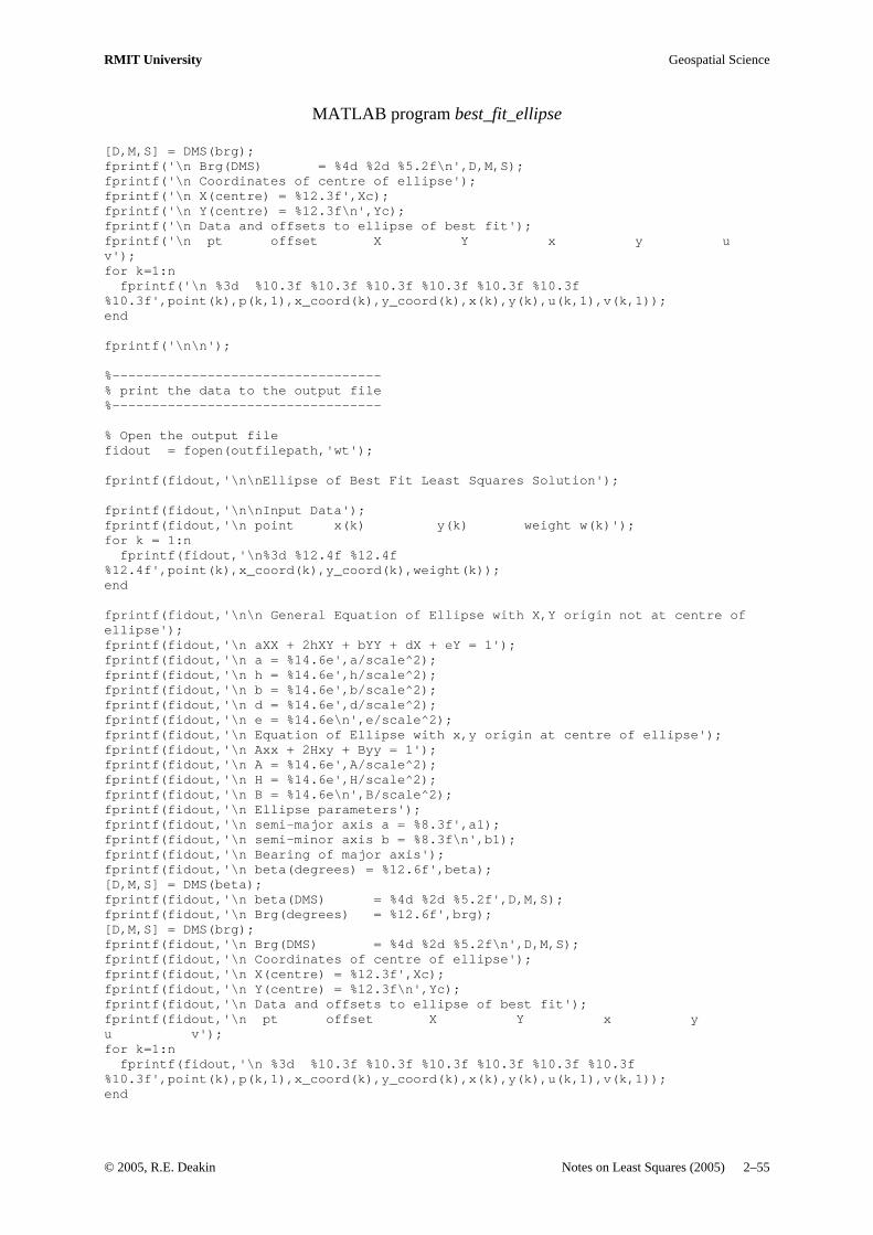
RMIT University Geospatial Science
MATLAB program best_fit_ellipse
[D,M,S] = DMS(brg); fprintf('\n Brg(DMS) = %4d %2d %5.2f\n',D,M,S); fprintf('\n Coordinates of centre of ellipse'); fprintf('\n X(centre) = %12.3f',Xc); fprintf('\n Y(centre) = %12.3f\n',Yc); fprintf('\n Data and offsets to ellipse of best fit'); fprintf('\n pt offset X Y x y u v'); for k=1:n fprintf('\n %3d %10.3f %10.3f %10.3f %10.3f %10.3f %10.3f %10.3f',point(k),p(k,1),x_coord(k),y_coord(k),x(k),y(k),u(k,1),v(k,1)); end fprintf('\n\n'); %---------------------------------- % print the data to the output file %---------------------------------- % Open the output file fidout = fopen(outfilepath,'wt'); fprintf(fidout,'\n\nEllipse of Best Fit Least Squares Solution'); fprintf(fidout,'\n\nInput Data'); fprintf(fidout,'\n point x(k) y(k) weight w(k)'); for k = 1:n fprintf(fidout,'\n%3d %12.4f %12.4f %12.4f',point(k),x_coord(k),y_coord(k),weight(k)); end fprintf(fidout,'\n\n General Equation of Ellipse with X,Y origin not at centre of ellipse'); fprintf(fidout,'\n aXX + 2hXY + bYY + dX + eY = 1'); fprintf(fidout,'\n a = %14.6e',a/scale^2); fprintf(fidout,'\n h = %14.6e',h/scale^2); fprintf(fidout,'\n b = %14.6e',b/scale^2); fprintf(fidout,'\n d = %14.6e',d/scale^2); fprintf(fidout,'\n e = %14.6e\n',e/scale^2); fprintf(fidout,'\n Equation of Ellipse with x,y origin at centre of ellipse'); fprintf(fidout,'\n Axx + 2Hxy + Byy = 1'); fprintf(fidout,'\n A = %14.6e',A/scale^2); fprintf(fidout,'\n H = %14.6e',H/scale^2); fprintf(fidout,'\n B = %14.6e\n',B/scale^2); fprintf(fidout,'\n Ellipse parameters'); fprintf(fidout,'\n semi-major axis a = %8.3f',a1); fprintf(fidout,'\n semi-minor axis b = %8.3f\n',b1); fprintf(fidout,'\n Bearing of major axis'); fprintf(fidout,'\n beta(degrees) = %12.6f',beta); [D,M,S] = DMS(beta); fprintf(fidout,'\n beta(DMS) = %4d %2d %5.2f',D,M,S); fprintf(fidout,'\n Brg(degrees) = %12.6f',brg); [D,M,S] = DMS(brg); fprintf(fidout,'\n Brg(DMS) = %4d %2d %5.2f\n',D,M,S); fprintf(fidout,'\n Coordinates of centre of ellipse'); fprintf(fidout,'\n X(centre) = %12.3f',Xc); fprintf(fidout,'\n Y(centre) = %12.3f\n',Yc); fprintf(fidout,'\n Data and offsets to ellipse of best fit'); fprintf(fidout,'\n pt offset X Y x y u v'); for k=1:n fprintf(fidout,'\n %3d %10.3f %10.3f %10.3f %10.3f %10.3f %10.3f %10.3f',point(k),p(k,1),x_coord(k),y_coord(k),x(k),y(k),u(k,1),v(k,1)); end
© 2005, R.E. Deakin Notes on Least Squares (2005) 2–55

RMIT University Geospatial Science
MATLAB program best_fit_ellipse
fprintf(fidout,'\n\n'); % Close the output file fclose(fidout); %------------------------------------------------------------------- % Call function 'ellipse' with parameters a,b,theta and receive back % X,Y coordinates whose origin is at the centre of the ellipse %------------------------------------------------------------------- [X,Y] = ellipse(a1,b1,beta); X = X + Xc; Y = Y + Yc; %------------------------------------------------------------------- % Set the X,Y coordinates of the major and minor axes of the ellipse %------------------------------------------------------------------- aX = [X(180) X(360)]; aY = [Y(180) Y(360)]; bX = [X(90) X(270)]; bY = [Y(90) Y(270)]; %------------------------------------------------- % plot the ellipse of Best Fit and the data points %------------------------------------------------- figure(1); clf(1); plot(X,Y,'r-',aX,aY,'b-',bX,bY,'b-'); hold on; plot(x_coord,y_coord,'k.'); axis equal; box off; % plot the point numbers inside the ellipse point_string=int2str(point); text(Xpt,Ypt,point_string); % anotate the plot title('Least Squares Ellipse of Best Fit') xlabel('X coordinate'); ylabel('Y coordinate');
© 2005, R.E. Deakin Notes on Least Squares (2005) 2–56
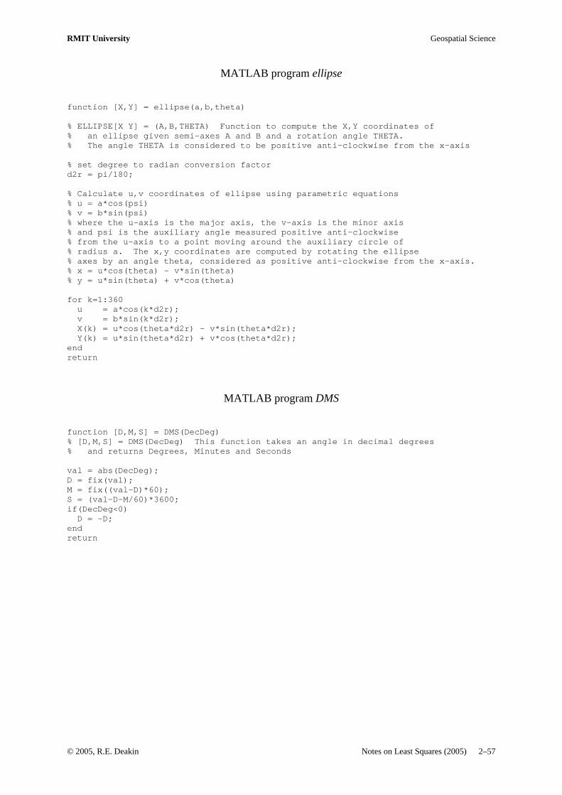
RMIT University Geospatial Science
MATLAB program ellipse
function [X,Y] = ellipse(a,b,theta) % ELLIPSE[X Y] = (A,B,THETA) Function to compute the X,Y coordinates of % an ellipse given semi-axes A and B and a rotation angle THETA. % The angle THETA is considered to be positive anti-clockwise from the x-axis % set degree to radian conversion factor d2r = pi/180; % Calculate u,v coordinates of ellipse using parametric equations % u = a*cos(psi) % v = b*sin(psi) % where the u-axis is the major axis, the v-axis is the minor axis % and psi is the auxiliary angle measured positive anti-clockwise % from the u-axis to a point moving around the auxiliary circle of % radius a. The x,y coordinates are computed by rotating the ellipse % axes by an angle theta, considered as positive anti-clockwise from the x-axis. % x = u*cos(theta) - v*sin(theta) % y = u*sin(theta) + v*cos(theta) for k=1:360 u = a*cos(k*d2r); v = b*sin(k*d2r); X(k) = u*cos(theta*d2r) - v*sin(theta*d2r); Y(k) = u*sin(theta*d2r) + v*cos(theta*d2r); end return
MATLAB program DMS
function [D,M,S] = DMS(DecDeg) % [D,M,S] = DMS(DecDeg) This function takes an angle in decimal degrees % and returns Degrees, Minutes and Seconds val = abs(DecDeg); D = fix(val); M = fix((val-D)*60); S = (val-D-M/60)*3600; if(DecDeg<0) D = -D; end return
© 2005, R.E. Deakin Notes on Least Squares (2005) 2–57