Learning from Summer
137
C O R P O R A T I O N Commissioned by Catherine H. Augustine, Jennifer Sloan McCombs, John F. Pane, Heather L. Schwartz, Jonathan Schweig, Andrew McEachin, Kyle Siler-Evans Online Technical Appendixes Learning from Summer
Transcript of Learning from Summer

C O R P O R A T I O N
Commissioned by
Catherine H. Augustine, Jennifer Sloan McCombs, John F. Pane, Heather L. Schwartz, Jonathan Schweig, Andrew McEachin, Kyle Siler-Evans
Online Technical Appendixes
Learning from Summer

Limited Print and Electronic Distribution Rights
This document and trademark(s) contained herein are protected by law. This representation of RAND intellectual property is provided for noncommercial use only. Unauthorized posting of this publication online is prohibited. Permission is given to duplicate this document for personal use only, as long as it is unaltered and complete. Permission is required from RAND to reproduce, or reuse in another form, any of its research documents for commercial use. For information on reprint and linking permissions, please visit www.rand.org/pubs/permissions.
The RAND Corporation is a research organization that develops solutions to public policy challenges to help make communities throughout the world safer and more secure, healthier and more prosperous. RAND is nonprofit, nonpartisan, and committed to the public interest.
RAND’s publications do not necessarily reflect the opinions of its research clients and sponsors.
Support RANDMake a tax-deductible charitable contribution at
www.rand.org/giving/contribute
www.rand.org
For more information on this publication, visit www.rand.org/t/RR1557
Published by the RAND Corporation, Santa Monica, Calif.
© Copyright 2016 RAND Corporation
R® is a registered trademark.

2
Preface
Research has determined that low-income students lose ground to more affluent peers over the summer. Other research has shown that some summer learning programs can benefit students, but we know very little about whether large, district-run, voluntary programs can improve student outcomes among low-income students.
To fill this gap, The Wallace Foundation launched the National Summer Learning Project in 2011. This six-year study offers the first-ever assessment of the effectiveness of large-scale, voluntary, district-run, summer learning programs serving low-income elementary students. The study, conducted by the RAND Corporation, uses a randomized controlled trial to assess the effects of district-run voluntary summer programs on academic achievement, social and emotional skills, and behavior over the near and long term. All students in the study were in the third grade as of spring 2013 and enrolled in a public school in one of five urban districts: Boston; Dallas; Duval County, Florida; Pittsburgh; or Rochester, New York.
The study follows these students from third to seventh grade. Our primary focus is on academic outcomes, but we also examine students’ social and emotional outcomes as well as behavior and attendance during the school year. We have also collected extensive data about the summer programs to help us examine how implementation is related to program effects.
This document includes the technical appendixes that accompany the third report resulting from the study, Learning from Summer: Effects of Two Years of Voluntary Summer Learning Programs on Low-Income Urban Youth (Augustine et al., 2016). These appendixes contain
• details of our randomization design (including treatment uptake, attrition, baseline equivalence of the treatment and control groups)
• details of our data collection processes and protocols (including characteristics of the participating students, descriptions of outcome measures, and a description of the observation process and protocol)
• a review of the extant literature on summer learning loss • a description of the mediators and moderators included in analyses (including detailed
information about how attendance and academic time on task were calculated) • analytic models used for estimating program effects • the complete results of all regression analyses.
This study is undertaken by RAND Education, a unit of the RAND Corporation that conducts research on prekindergarten, K–12, and higher education issues, such as preschool quality rating systems, assessment and accountability, teacher and leader effectiveness, school improvement, out-of-school time, educational technology, and higher education cost and completion.

3
This study is sponsored by The Wallace Foundation, which seeks to support and share effective ideas and practices to foster improvements in learning and enrichment for disadvantaged children and the vitality of the arts for everyone. Its current objectives are to improve the quality of schools, primarily by developing and placing effective principals in high-need schools; improve the quality of and access to after-school programs through coordinated city systems and by strengthening the financial management skills of providers; reimagine and expand learning time during the traditional school day and year, as well as during the summer months; expand access to arts learning; and develop audiences for the arts. For more information and research on these and other related topics, visit The Foundation’s Knowledge Center at www.wallacefoundation.org.

4
Table of Contents
Preface ............................................................................................................................................. 2 Figures ............................................................................................................................................. 7 Tables .............................................................................................................................................. 8 Abbreviations ................................................................................................................................ 11 Appendix A: Randomization Design and Implementation ........................................................... 12
Randomization of Students to Treatment and Control Groups ................................................. 12 Stratification Plan ............................................................................................................................... 12 Writing the Computer Code for the Randomization .......................................................................... 14 Siblings ............................................................................................................................................... 15
Program Uptake ........................................................................................................................ 15 Minimum Detectable Effect Sizes ............................................................................................ 17 Attrition ..................................................................................................................................... 17
Fall 2013 ............................................................................................................................................. 18 Spring 2014 ......................................................................................................................................... 18 Fall 2014 ............................................................................................................................................. 19 Spring 2015 ......................................................................................................................................... 19
Balance of the Treatment and Control Groups After Attrition ................................................. 20 Fall 2013 ............................................................................................................................................. 20 Spring 2014 ......................................................................................................................................... 21 Fall 2014 ............................................................................................................................................. 24 Spring 2015 ......................................................................................................................................... 25
Appendix B: Data Collection ........................................................................................................ 28 Characteristics of Students in the Sample ................................................................................. 28 Academic Achievement ............................................................................................................ 29
Spring Tests ........................................................................................................................................ 29 Fall Tests ............................................................................................................................................. 33 End-of-Course Grades ........................................................................................................................ 37 Suspensions ........................................................................................................................................ 42 School-Year Attendance ..................................................................................................................... 43
Social-Emotional Outcomes ..................................................................................................... 44 Student Survey Responses ........................................................................................................ 46 Summer Teacher Survey ........................................................................................................... 48 Classroom Observations ........................................................................................................... 54
Inter-Rater Agreement ........................................................................................................................ 61 Daily Site Observation ........................................................................................................................ 62
Summer Student Attendance .................................................................................................... 62

5
Summer Program Costs ............................................................................................................ 63 Cost Data Collection and Cleaning .................................................................................................... 63
Student Summer Activities Questionnaire (Fall 2014) ............................................................. 66 Summer 2014 Academic Teacher Survey ................................................................................ 67 Summer 2014 Classroom Observation Protocols ..................................................................... 77
Overview ............................................................................................................................................ 77 Academic Class Segments .................................................................................................................. 78 Enrichment Class Segments ............................................................................................................... 80 Evidence of Classroom Practices ....................................................................................................... 81 Evidence of Summer School Climate ................................................................................................. 82 Overall Reactions ............................................................................................................................... 83
Data Request Form for Summer 2014 District-Level Costs ..................................................... 84 Summer 2014 Daily Site Observation Protocol ................................................................................. 87
Appendix C: Recent Studies on Summer Learning ...................................................................... 90 Summer Learning Loss ............................................................................................................. 90
Income-Based and Race-Based Gaps in Learning over the Summer ................................................. 92 Extent of Summer Learning Loss as Children Age ............................................................................ 93
Summer Program Effectiveness ................................................................................................ 94 Academic Outcomes ........................................................................................................................... 94 Nonacademic Outcomes ..................................................................................................................... 95 Long-Term Effects ............................................................................................................................. 95 Variation in Effectiveness of Summer Learning Programs ................................................................ 95 Components of Quality Summer Learning Programs ........................................................................ 97
Conclusions ............................................................................................................................... 99 Appendix D: Hypothesized Mediators and Moderators of Summer Program Effects ............... 100
Attendance and Academic Time on Task ............................................................................... 100 Attendance ........................................................................................................................................ 100 Academic Time on Task ................................................................................................................... 101 Cumulative Measures of Attendance and Academic Time on Task ................................................ 103
Creation of Relative Opportunity for Individual Attention .................................................... 103 Scales Created from Teacher Survey and Classroom Observation Data ................................ 105
Quality of Instruction ........................................................................................................................ 108 Appropriateness of the (Mathematics/Language Arts) Curriculum ................................................. 109 Good Fit of the (Mathematics/Language Arts) Curriculum ............................................................. 109 Student Discipline and Order Scale .................................................................................................. 110 Positive School Climate .................................................................................................................... 111 The Daily Climate Scale ................................................................................................................... 112
Appendix E: Statistical Analysis ................................................................................................ 113 Analysis Plan .......................................................................................................................... 113
Preferred Random-Effects Model ..................................................................................................... 113 Attendance and Academic Time-on-Task Analysis ......................................................................... 115

6
Robustness Checks ........................................................................................................................... 115 Analysis of Treatment Effect on the Treated .......................................................................... 116 Multiple Hypotheses Testing .................................................................................................. 116 Meta-Analysis ......................................................................................................................... 118 Linear Probability Models ...................................................................................................... 118
Appendix F: Results from Regression Models ........................................................................... 120 References ................................................................................................................................... 128

7
Figures
B.1. Histograms of Standardized Scale Scores on the State Spring 2014 Mathematics Assessments .......................................................................................................................... 30
B.2. Histograms of Standardized Scale Scores on the State Spring 2014 LA Assessments ......... 31 B.3. Histograms of Standardized Scale Scores on the State Spring 2015 Mathematics
Assessments .......................................................................................................................... 32 B.4. Histograms of Standardized Scale Scores on the State Spring 2015 LA Assessments ......... 33 B.5. Fall 2013 Score Distributions ................................................................................................ 36 B.6. Fall 2014 Score Distributions ................................................................................................ 37 B.7. Histograms of Rescaled SY 2013–2014 Mathematics Course Grades for Each District ...... 39 B.8. Histograms of Rescaled SY 2013–2014 Language Arts Course Grades for Each
District ................................................................................................................................... 40 B.9. Histograms of Rescaled SY 2014–2015 Mathematics Course Grades for Each District ...... 41 B.10. Histograms of Rescaled SY 2014–2015 Language Arts Course Grades for Each
District ................................................................................................................................... 42 D.1. Distributions of the Relative Opportunity for Individual Attention Variable
(Fall 2013) ........................................................................................................................... 105 D.2. Distributions of the Relative Opportunity for Individual Attention Variable
(Fall 2014) ........................................................................................................................... 105

8
Tables
A.1. Impact of Treatment Assignment on the Likelihood of Program Participation .................... 16 A.2. Impact of Treatment Assignment on the Likelihood of Program Participation .................... 16 A.3. Minimum Detectable Effect Sizes for Intent-to-Treat Analyses of Near-Term Outcomes ........ 17 A.4. Assessment of Differential Attrition (Fall 2013 Outcomes) ................................................. 18 A.5. Assessment of Differential Attrition (Spring 2014 Outcomes) ............................................ 19 A.6. Assessment of Differential Attrition (Fall 2014 Outcomes) ................................................. 19 A.7. Assessment of Differential Attrition (Spring 2015 Outcomes) ............................................ 20 A.8. Assessment of Treatment-Control Group Balance After Attrition
(Fall 2013 Mathematics) ....................................................................................................... 20 A.9. Assessment of Treatment-Control Group Balance After Attrition (Fall 2013 Reading) ...... 21 A.10. Assessment of Treatment-Control Group Balance After Attrition
(Spring 2014 Mathematics) ................................................................................................... 22 A.11. Assessment of Treatment-Control Group Balance After Attrition (Spring 2014 LA) ....... 22 A.12. Assessment of Treatment-Control Group Balance After Attrition
(Spring 2014 Attendance and Suspension) ........................................................................... 23 A.13. Assessment of Treatment-Control Group Balance After Attrition
(Fall 2014 Mathematics) ....................................................................................................... 24 A.14. Assessment of Treatment-Control Group Balance After Attrition (Fall 2014 Reading) .... 24 A.15. Assessment of Treatment-Control Group Balance After Attrition (Spring 2015
Mathematics) ......................................................................................................................... 25 A.16. Assessment of Treatment-Control Group Balance After Attrition (Spring 2015 LA) ....... 26 A.17. Assessment of Treatment-Control Group Balance After Attrition (Attendance and
Suspension) ........................................................................................................................... 27 B.1. Characteristics of Students in the Experiment ...................................................................... 28 B.2. Response Rates for Fall Mathematics and Reading Assessments, 2013 and 2014 ............... 35 B.3. Description of Course Grading Systems ............................................................................... 38 B.4. Domains in District B’s Language Arts and Mathematics Grading Systems ....................... 38 B.5. Districtwide Suspension Rates for SYs 2013–2014 and 2014–2015 .................................... 43 B.6. School-Year Attendance Data for SYs 2013–2014 and 2014–2015 by District ................... 43 B.7. DESSA-RRE Social-Emotional Behavior Scales ................................................................. 45 B.8. Summer 2013 Student Survey Responses ............................................................................. 46 B.9. Summer 2014 Student Survey Responses ............................................................................. 47 B.10. Response Rates on Summers 2013 and 2014 Academic Teacher Surveys ......................... 48 B.11. Summer 2013 Academic Teachers’ Views of Their Summer Program .............................. 49 B.12. Summer 2013 Academic Teachers’ Views of PD and Program Curricula ......................... 50

9
B.13. Summer 2014 Academic Teachers’ Views of Their Summer Program by District ............ 51 B.14. Summer 2014 Academic Teachers’ Views of the PD and Curriculum for Their
Summer Program by District ................................................................................................ 52 B.15. Number of Classroom Observations Each Summer ............................................................ 55 B.16. Overview of Instructional Time by District in Summer 2014 ............................................ 56 B.17. Summer 2014 Mathematics Practices That Support Student Engagement by District ....... 56 B.18. Summer 2014 Desirable Mathematics Classroom Practices by District ............................. 57 B.19. Summer 2014 Undesirable Mathematics Classroom Practices by District ......................... 57 B.20. Summer 2014 LA Practices That Support Student Engagement by District ...................... 58 B.21. Summer 2014 Desirable LA Classroom Practices by District ............................................ 58 B.22. Summer 2014 Undesirable LA Classroom Practices by District ........................................ 59 B.23. Summer 2014 Enrichment Practices That Support Student Engagement by District ......... 59 B.24. Summer 2014 Desirable Enrichment Classroom Practices by District ............................... 60 B.25. Summer 2014 Undesirable Enrichment Classroom Practices by District ........................... 61 B.26. RAND Daily Site Observation by District .......................................................................... 62 B.27. Line Item Expenses Included in Each of the Six Cost Categories ...................................... 64 D.1. Distribution of Instructional Hours That Treatment Group Students Received ................. 102 D.2. Thresholds for Attendance and Academic Time-on-Task Categories ................................ 102 D.3. Distribution of Average Language Arts/Mathematics Class Sizes ..................................... 104 D.4. Summary Statistics of Hypothesized Mediators ................................................................. 107 D.5. Mathematics/Language Arts Instructional Quality Items and Internal Consistency
Reliability Estimates ........................................................................................................... 108 D.6. Appropriateness of Mathematics/Language Arts Curriculum Scale Items and Internal
Consistency Reliability Estimates ....................................................................................... 109 D.7. Student Discipline and Order Scale Items, and Internal Consistency Reliability
Estimates ............................................................................................................................. 110 D.8. Site Climate Scale Items and Internal Consistency Reliability Estimates .......................... 111 D.9. Daily Climate Scale items ................................................................................................... 112 E.1. Number of Hypothesis Test for Each Outcome Domain for Each Study Time Point ......... 117 F.1. ITT Results, Overall ............................................................................................................ 120 F.2. Counts of Students Participating in ITT Analyses .............................................................. 120 F.3. Counts of Students Participating in Subgroup Analyses (Fall Analyses) ............................ 121 F.4. Results of Subgroup Analyses ............................................................................................. 122 F.5. Results of Subscale Analyses .............................................................................................. 122 F.6. Results of Treatment-on-the-Treated Analyses ................................................................... 123 F.7. Nonexperimental Linear Effect of Attendance and Academic Time on Task ..................... 123 F.8a. Nonexperimental Effect of Attendance Categories ........................................................... 123 F.8b. Nonexperimental Effect of Academic Time on Task Categories ...................................... 125 F.9. Nonexperimental Effects of Camp Attendance According to Student Survey .................... 125

10
F.10. Nonexperimental Estimates of the Effect of Relative Opportunity for Instruction ........... 126 F.11. Nonexperimental Estimates of Moderation ....................................................................... 126

11
Abbreviations
CBO community-based organizations
DESSA-RRE Devereux Student Strengths Assessment–RAND Research Edition
ECLS-K Early Childhood Longitudinal Study Kindergarten
ELL English language learner
FRPL free and reduced-price lunch
GMADE Group Mathematics Assessment and Diagnostic Evaluation
GRADE Group Reading Assessment and Diagnostic Evaluation
IEP individualized education plan
ITT intent-to-treat
LA language arts
LPM linear probability model
MDES minimum detectable effect size
NWEA Northwestern Evaluation Association
OLS ordinary least squares
SD standard deviation
SE standard error
SES socioeconomic status
SY school year
TOT treatment on the treated

12
Appendix A: Randomization Design and Implementation
This appendix discusses the details of how randomization was conducted, the statistical power for detecting treatment effects, the rates of attrition for each outcome, and the comparability of the treatment and control groups after attrition.
Randomization of Students to Treatment and Control Groups
In each district, parents submitted applications for their children to participate in the summer program along with their consent for children’s participation in the study. Students admitted to the programs were assigned to a specific summer site, typically through geographic feeder patterns.
Stratification Plan
Our thinking about how to design the experiment was strongly influenced by Imbens (2011), who discusses the methodological considerations that should be made when designing a randomized controlled trial experiment. He shows that partitioning the sample into strata (groups of individuals with similar characteristics) and then randomizing within strata is preferable to randomizing without first creating strata, from the standpoint of maximizing statistical power, and that the benefits of randomization are strongest when (1) there are “relatively many and small strata” and (2) the strata are based on covariates that are strongly related to the outcome of interest.
With these considerations in mind, we constructed strata for the experiment based on the following variables:
• district • third-grade school • English language learner (ELL) status in third grade • race/ethnicity: Hispanic, African American, other1 • eligibility for either free or reduced-price lunch (FRPL) in third grade • prior achievement.
We chose these variables for several reasons. First, these are variables for which each district in the study maintains records. Second, these are all factors that are well known to be strong predictors of student achievement. Finally, such variables as ELL status are related to the type of test a student takes or whether a student is tested at all. As we will discuss, we conducted
1 For the purposes of the stratification, Hispanic will refer to students of Hispanic origin of any race and African American will refer to non-Hispanic black students.

13
robustness checks where we limited the sample to particular student subgroups, including students tested only in English, since the testing conditions may not be comparable for ELL students. Since some researchers advocate stratifying on variables that will be used in subgroup analyses (Duflo, Glennerster, and Kremer, 2007), we thought it important to include these factors in the definition of the randomization strata.
Stratifying by prior achievement was important for our experiment, but it was unclear which achievement measure to use for this. In some districts, systematic testing begins in spring of the second grade, whereas other districts begin with benchmark assessments in the fall of third grade. Further, students are tested in multiple subjects. We stratified on the most-recent test scores that were available for all students. In districts where all students were tested in reading and mathematics, we used the average of these two subjects as the stratifying variable. A different approach was used in sites that administered some of their tests in Spanish to Spanish-speaking ELL students. For example, in Dallas, the stratification was based on mathematics tests, which are administered in English to all students.
While Imbens (2011) argues in favor of using strata with relatively few students, he also points out that there are analytic challenges associated with having few (e.g., two) students per strata.2 A practical limitation of having strata with too few observations is that if students drop out of the sample because of attrition and only control or treatment students are left, the entire strata must be dropped from the analysis. Thus, we defined each stratum to have about 15–30 students. For example, with ten students assigned to treatment in a stratum, it was unlikely that all of the students would attrit from the study or be treatment no-shows.3
The basic algorithm used to generate the strata was as follows:
1. We fully stratified the summer program enrollees into cells defined by district-school-race-ELL-FRPL-achievement. For this step, achievement is a binary variable with half the enrollees in a district in a high-achievement group and the other half in a low-achievement group.4 Since a goal of the study was to examine effects by higher- and lower-achieving students, it was important to stratify the sample in this way so that the high- and low-achievement subgroups coincided with the strata.
2. For cells defined in Step 1 with at least one but fewer than 15 students, we aggregated cells until each had at least 15 students. Cells were aggregated in the following order: (a) FRPL eligibility, (b) race, (c) ELL status, and (d) binary achievement. We did not collapse schools to ensure that within each school the proportion assigned to treatment
2 Specifically, it was impossible to compute the variance of the within-strata treatment effect estimate. The estimated variance of the treatment effect in the case with just two observations per strata (i.e., a paired randomization design) would be biased upward for the true variance of the estimated treatment effect. 3 Suppose that five students dropped out of the study (which would be higher than the long-run attrition rate of 30 percent that we assumed). If the no-show rate were 30 percent, then the probability that all five of the nondropouts were no-shows would be only about 0.002. 4 Students with missing baseline achievement data were assigned to the low-achievement strata. See our discussion for additional sensitivity checks that were performed to handle missing baseline data.

14
was near the intended proportion (as close as possible considering rounding). To see how this worked, suppose that the cell for FRPL students who are African American, ELL, low-achievement, and in school A contained only five students. The first step in aggregating cells would be to pool across the FRPL category (essentially eliminating the FRPL criteria) to form a cell for students who were African American, ELL, low-achievement, and in school A. If this new cell still had fewer than 15 students, then the next step would be to form a cell for students who were in the African American or other race categories (i.e., pool across the smallest race categories), and if further pooling were necessary, to pool again by race, as necessary until all race categories are pooled, and then to pool by ELL, etc. This process was repeated until students were all assigned to cells with at least 15 students or to cells at the school level that could not be further aggregated.
The ordering of covariates for the aggregation reflected how important we thought each variable was in the stratification; we aggregated on less-important variables first. We placed the greatest importance on the sending school for programmatic reasons: Stratifying on the school ensured that no sending school would have a disproportionately large or small proportion of students assigned to treatment, helping to make clear that all stakeholders were being treated fairly by the randomization process. The second tier of importance was given to the achievement and ELL variables because we examined treatment effects by subgroups according to these variables. Finally, FRPL and race were included in the stratification plan because they were strongly associated with student outcomes; however, they received the lowest priority.
3. For cells that, at the end of Step 2, contained more than 30 students, we stratified them further by the achievement variable to form as many cells as possible that contained at least 15 students. For instance, if a cell had 65 students at the end of Step 2, we formed three cells with 16 students each and one with 17 students.5 We used achievement to further stratify the larger cells because prior achievement was the strongest predictor of future achievement, so forming strata in this way maximized statistical power.
Writing the Computer Code for the Randomization
We used Stata.do files to carry out the stratified random assignment. We assigned percentage P of student applicants to the treatment group. P varied across districts and summer sites within a district, ranging between 50 percent and 60 percent. We capped P within any summer site at 70 percent.
Within each strata, P percent of students were assigned to the treatment group. For strata where the number of observations did not enable exactly P percent to be assigned to treatment,
5 More formally, for a cell, c, with Nc students, we formed k=int(Nc/15) subcells, with int(Nc/k) students in k–mod(Nc,k) cells and int(Nc/k)+1 students in mod(Nc,k) cells.

15
the number of students assigned to treatment was equal to round(P*Nc), where Nc was the number of students in strata c. In this way, whether there was slightly more or less than P percent of students assigned to treatment varied across strata but this variation was random.
To do the actual random assignment, we used the STATA pseudorandom number generator. Specifically, we assigned each student a random number drawn from a uniform distribution on the interval (0,1). Students were sorted according to this number so that the sort order of the students was random. After sorting the data in this way, within each strata, students whose sort order was less than or equal to Ntc were assigned to treatment, where Ntc is the number of students in strata c assigned to treatment. The strata identifier, c, was stored with each record for use in future analyses.
Siblings
It could be disruptive to families if one or more of their children were admitted to the program and one or more were not admitted. In all districts that requested that we account for siblings, we adopted procedures to keep together all siblings that made valid applications to the program.6 Where one of the siblings was in third grade and the remaining siblings were in other grades, the admission decision for all of the children was based on the third-grader’s randomly assigned admission status. Where there were multiple siblings in the third-grade sample, the siblings were randomly assigned as a group so that all received admission or all were denied admission.
Program Uptake Next, we discuss estimates of the impact of the randomized treatment assignment on
participation in the summer programs in both 2013 and 2014. We examine uptake during each of the two summers and examine uptake across the two years combined. Participation in the summer program is defined as attending at least one day of the relevant program offering period (summer 1, summer 2, or any time over the two summers). With perfect compliance to the experimental protocol, treatment assignment and program uptake would be the same. However, as Table A.1 indicates, not all students admitted to the summer programs actually attended, and some students assigned to the control group attended the program.7 In the second year, slightly more than half the students who were admitted to summer programs actually attended. Overall, nearly 85 percent of admitted students attended at least one day of the summer program in either summer.
6 Siblings were not considered when randomizing for Boston, by the decision of the district. 7 The uptake rates by treatment assignment status were virtually identical for the sample of mathematics and LA non-attriters. In Dallas, some students assigned to the control group were nonetheless admitted to the program. There were a handful of other such “crossover” control group students in other districts as well.

16
Table A.1. Impact of Treatment Assignment on the Likelihood of Program Participation
Attendance Period
Program Uptake Among Students Assigned to
Treatment Group
Program Uptake Among Students Assigned to
Control Group
Difference in Uptake Between Treatment and
Control Groups
Summer 1 (2013) 0.799 0.047 0.752 Summer 2 (2014) 0.518 0.008 0.510 Either summer 0.842 0.051 0.791
Table A.2 shows linear probability model estimates of the impact of treatment assignment on
program uptake. Standard errors were calculated using the Eicker-Huber-White sandwich estimator (e.g., using Stata’s “robust” command) that is robust to heteroskedasticity (Eicker, 1967; Huber, 1967; White, 1980). For Year 1, the results indicate that assignment to be eligible for the program increased the likelihood of attending the program for at least one day by 74 percentage points. For Year 2, the results indicated that assignment to be eligible for the program increased the likelihood of attending the program for at least one day by nearly 50 percentage points. Overall, across both years, assignment to be eligible for the program increased the likelihood of attending the program for at least one day by 79 percentage points. Where we present treatment-on-the-treated (TOT) effect estimates, we report instrumental variable estimates of the impact of summer program attendance for the set of students whose summer program attendance was affected by the experimental assignment, which are equal to the intent-to-treat (ITT) estimates scaled up by the inverse of the estimates in Table A.2.
Table A.2. Impact of Treatment Assignment on the Likelihood of Program Participation
Assignment Estimate Standard Error p value
Year 1 Only strata fixed effects 0.741 0.008 0.000 All student-level covariates 0.741 0.008 0.000
Year 2 Only strata fixed effects 0.498 0.010 0.000 All student-level covariates 0.497 0.010 0.000
Both years Only strata fixed effects 0.791 0.008 0.000 All student-level covariates 0.791 0.008 0.000
NOTE: Student-level covariates are standardized mathematics and reading scores from the state’s spring third-grade assessments and fall third-grade diagnostic tests; classroom average of these pretests; dummy variables for FRPL, African American, Hispanic, ELL, special education and male classifications; and dummy variables for missing pretest scores.
17
Minimum Detectable Effect Sizes To estimate the statistical power of the study during the design phase, we applied formulas
for experiments in which treatment students were clustered in classes, and calculated the minimum detectable effect size (MDES) the study would be able to identify with 80 percent probability using a two-tailed test and a 0.05 level of significance. To perform these calculations, we estimated several parameters using existing empirical data from pilot work in summers 2011 and 2012, as well as the published literature. These estimates were uncertain, and as a general rule, we chose conservative values that would produce higher, rather than lower, MDES estimates.
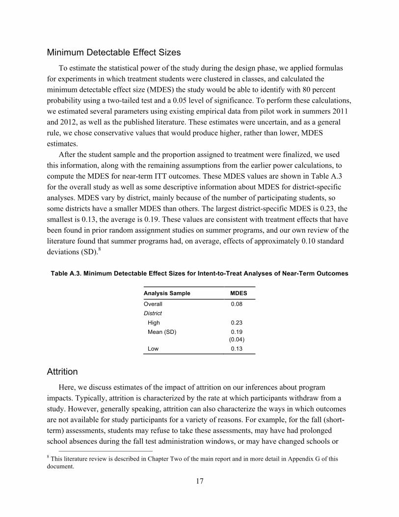
After the student sample and the proportion assigned to treatment were finalized, we used this information, along with the remaining assumptions from the earlier power calculations, to compute the MDES for near-term ITT outcomes. These MDES values are shown in Table A.3 for the overall study as well as some descriptive information about MDES for district-specific analyses. MDES vary by district, mainly because of the number of participating students, so some districts have a smaller MDES than others. The largest district-specific MDES is 0.23, the smallest is 0.13, the average is 0.19. These values are consistent with treatment effects that have been found in prior random assignment studies on summer programs, and our own review of the literature found that summer programs had, on average, effects of approximately 0.10 standard deviations (SD).8
Table A.3. Minimum Detectable Effect Sizes for Intent-to-Treat Analyses of Near-Term Outcomes
Analysis Sample MDES
Overall 0.08 District
High 0.23 Mean (SD) 0.19
(0.04) Low 0.13
Attrition Here, we discuss estimates of the impact of attrition on our inferences about program
impacts. Typically, attrition is characterized by the rate at which participants withdraw from a study. However, generally speaking, attrition can also characterize the ways in which outcomes are not available for study participants for a variety of reasons. For example, for the fall (short-term) assessments, students may refuse to take these assessments, may have had prolonged school absences during the fall test administration windows, or may have changed schools or
8 This literature review is described in Chapter Two of the main report and in more detail in Appendix G of this document.

18
school districts before the administration. For the spring outcomes (course grades, state assessments, school-year suspension, and school-year attendance), students may have moved out of district, or may have moved within the district to a school that does not report these data to local education agencies (for example, movement to a charter school). In the remainder of this section, we discuss attrition in this general way for each data collection time point (fall 2013, spring 2014, fall 2014, and spring 2015) and for each relevant outcome.
Fall 2013
As described in more detail in Appendix B, fall 2013 mathematics outcomes were available for 5,127 students, and reading outcomes were available for 5,101 students. These represent attrition rates of 9.1 percent and 9.5 percent, respectively.
To test whether there was differential attrition in the treatment and control groups, we ran linear probability models that predicted attrition based on the treatment indicator. The first model included fixed effects for random assignment strata but no other covariates; the second also included the student-level covariates already discussed. Standard errors were calculated using the Huber-Eicker-White sandwich estimator that is robust to heteroskedasticity. The results show that treatment group students and control group students do not have distinguishably differential tendencies to attrit (see Table A.4).
Table A.4. Assessment of Differential Attrition (Fall 2013 Outcomes)
Subject of Study Only Strata Fixed Effects
Estimate (SE) All Student-Level Covariates
Estimate (SE)
Mathematics –0.012 (0.008) –0.012 (0.008) Reading –0.010 (0.008) –0.007 (0.008)
NOTE: SE = standard error. Student-level covariates are standardized mathematics and reading scores from the state’s spring third-grade assessments and fall third-grade diagnostic tests; classroom average of these pretests; dummy variables for FRPL, African American, Hispanic, ELL, special education and male classifications; and dummy variables for missing pretest scores.
Spring 2014
Spring 2014 outcomes include state standardized tests (mathematics and language arts [LA]), end-of-year course grades (mathematics and LA), school-year suspensions, and school-year attendance rates. Mathematics state assessment data was available for 90.6 percent of students (N = 5,138); LA state assessment data was available for 90.8 percent of students (N = 5,130). Course grades were available for 89.8 percent and 89.9 percent of students in mathematics (N = 5,062) and LA (N = 5,065), respectively. Suspension data was available for 94.4 percent of students (N = 5,331), and attendance data was available for 94.3 percent of students (N = 5,329). The results in Table A.5 show that treatment group students and control group students do not have distinguishably differential tendencies to attrit.

19
Table A.5. Assessment of Differential Attrition (Spring 2014 Outcomes)
Assessment Only Strata Fixed Effects
Estimate (SE) All Student-Level Covariates
Estimate (SE)
Mathematics state test –0.005 (0.008) –0.007 (0.008) LA state test –0.005 (0.008) –0.005 (0.008) Mathematics grades –0.013 (0.008) –0.013 (0.008) LA grades –0.010 (0.008) –0.009 (0.008) Suspension in school year (SY) 2013–2014 –0.002 (0.006) –0.001 (0.006) Attendance in SY 2013–2014 –0.003 (0.006) –0.003 (0.006)
NOTE: Student-level covariates are standardized mathematics and reading scores from the state’s spring third-grade assessments and fall third-grade diagnostic tests; classroom average of these pretests; dummy variables for FRPL, African American, Hispanic, ELL, special education and male classifications; and dummy variables for missing pretest scores.
Fall 2014
Fall 2014 mathematics outcomes were available for 4,505 students, and reading outcomes were available for 4,484 students. These represent attrition rates of 20.1 percent and 20.5 percent, respectively. The results show that differences between treatment and control group students are indistinguishable from zero (see Table A.6).
Table A.6. Assessment of Differential Attrition (Fall 2014 Outcomes)
Subject of Study Only Strata Fixed Effects
Estimate (SE) All Student-Level Covariates
Estimate (SE)
Mathematics –0.006 (0.011) –0.006 (0.011) Reading –0.007 (0.011) –0.005 (0.011)
NOTE: Student-level covariates are standardized mathematics and reading scores from the state’s spring third-grade assessments and fall third-grade diagnostic tests; classroom average of these pretests; dummy variables for FRPL, African American, Hispanic, ELL, special education and male classifications; and dummy variables for missing pretest scores.
Spring 2015
Spring 2015 outcomes include state standardized tests (mathematics and LA), end-of-year course grades (mathematics and LA), school-year suspensions, and school-year attendance rates. Mathematics state assessment data was available for 62.3 percent of students (N = 4,301); LA state assessment data was available for 62.9 percent of students (N = 4,337). Course grades were available for 79.1 percent and 79.2 percent of students in mathematics (N = 4,458) and LA (N = 4,464), respectively. Suspension data was available for 85 percent of students (N = 4,782) and attendance data was available for 85 percent of students (N = 4,782). The results in Table A.7 show that treatment group students and control group students do not have distinguishably differential tendencies to attrit.

20
Table A.7. Assessment of Differential Attrition (Spring 2015 Outcomes)
Assessment Measure Only Strata Fixed Effects
Estimate (SE) All Student-Level Covariates
Estimate (SE)
Mathematics state test –0.003 (0.010) –0.002 (0.010) LA state test –0.004 (0.010) –0.002 (0.010) Mathematics grades –0.006 (0.011) –0.005 (0.010) LA grades –0.008 (0.011) –0.005 (0.010) Suspension in SY 2014–2015 –0.008 (0.009) –0.007 (0.009) Attendance in SY 2014–2015 –0.008 (0.010) –0.007 (0.009)
NOTE: Student-level covariates are standardized mathematics and reading scores from the state’s spring third-grade assessments and fall third-grade diagnostic tests; classroom average of these pretests; dummy variables for FRPL, African American, Hispanic, ELL, special education and male classifications; and dummy variables for missing pretest scores.
Balance of the Treatment and Control Groups After Attrition Next, we assessed balance in the observable characteristics of the treatment and control
groups that were retained in the analytic sample after attrition. As above, these results are presented for each data collection time point (fall 2013, spring 2014, fall 2014, and spring 2015) and for each relevant outcome.
Fall 2013
Table A.8 shows the results for mathematics from statistical models that predicted assignment to the treatment group based on each student-level achievement or demographic variable, fit one at a time, controlling for the strata used in random assignment. Table A.9 shows the corresponding results for reading.
Table A.8. Assessment of Treatment-Control Group Balance After Attrition (Fall 2013 Mathematics)
Characteristics Estimate Standard Error p value
2012 benchmark mathematics assessment 0.009 0.009 0.353 2013 state mathematics assessment 0.015 0.008 0.061 2012 benchmark reading assessment 0.000 0.009 0.992 2013 state reading state assessment 0.007 0.008 0.341 Eligible for free or reduced-price lunch 0.002 0.026 0.938 Black 0.012 0.019 0.509 Hispanic 0.004 0.022 0.845 English-language learner –0.007 0.020 0.721 Special education student (gifted excluded) 0.043 0.025 0.088 Student is male –0.003 0.015 0.821 NOTE: Table shows results of univariate models (with strata fixed effects) using each covariate to predict treatment in the sample remaining after attrition. A likelihood ratio test of these variables’ joint ability to predict treatment assignment in a multivariate model yielded a p value of 0.540.

21
Table A.9. Assessment of Treatment-Control Group Balance After Attrition (Fall 2013 Reading)
Characteristic Estimate Standard Error p value
2012 benchmark mathematics assessment 0.011 0.009 0.228 2013 state mathematics assessment 0.018 0.008 0.025 2012 benchmark reading assessment 0.003 0.009 0.760 2013 state reading state assessment 0.010 0.008 0.200 Eligible for free or reduced-price lunch –0.001 0.026 0.980 Black 0.017 0.019 0.372 Hispanic –0.001 0.022 0.972 English-language learner –0.013 0.020 0.505 Special education student (gifted excluded) 0.044 0.025 0.078 Student is male –0.006 0.015 0.704 NOTE: Table shows results of univariate models (with strata fixed effects) using each covariate to predict treatment in the sample remaining after attrition. A likelihood ratio test of these variables’ joint ability to predict treatment assignment in a multivariate model yielded a p value of 0.322.
In both cases, the differences between the retained treatment and control groups were
generally small and not significant. An exception was that, in both mathematics and reading, the treatment group had slightly higher scores on the 2013 state assessment, by 0.015 and 0.018, respectively. The difference was marginally significant in mathematics and significant at the p < 0.05 level in reading. These differences were small with to what is considered acceptable in a valid experiment.9
Spring 2014
We then assessed balance in the observable characteristics of the treatment and control groups that were retained in the analytic sample for spring 2014 outcomes. Tables A.10–A.12 show the balance for state assessments and course grades in mathematics and LA, as well as for attendance and suspension outcomes, and help us to understand whether there is adequate evidence that the treatment and control groups are equivalent at baseline, after accounting for attrition. Again, balance was appraised using statistical models that predicted assignment to the treatment group based on each student-level achievement or demographic variable, fit one at a time, controlling for the strata used in random assignment.
9 For example, the What Works Clearinghouse (U.S. Department of Education, 2014) sets a limit of 0.25 for pretreatment group differences when the variable will be used as a covariate in outcomes models, as we did here.

22
Table A.10. Assessment of Treatment-Control Group Balance After Attrition (Spring 2014 Mathematics)
Characteristic Estimate Standard Error p value
Spring Standardized Assessments 2012 benchmark mathematics assessment 0.005 0.009 0.557 2013 state mathematics assessment 0.012 0.008 0.628 2012 benchmark reading assessment 0.000 0.009 0.945 2013 state reading state assessment 0.004 0.008 0.628 Eligible for free or reduced-price lunch 0.006 0.025 0.828 Black 0.003 0.019 0.874 Hispanic 0.012 0.022 0.589 English-language learner –0.009 0.020 0.647 Special education student (gifted excluded) 0.037 0.026 0.150 Student is male 0.002 0.015 0.904
Spring Course Grades 2012 benchmark mathematics assessment 0.007 0.009 0.412 2013 state mathematics assessment 0.014 0.008 0.102 2012 benchmark reading assessment –0.000 0.008 0.966 2013 state reading state assessment 0.004 0.008 0.637 Eligible for free or reduced-price lunch 0.011 0.026 0.681 Black 0.009 0.019 0.638 Hispanic 0.006 0.022 0.802 English-language learner –0.009 0.020 0.659 Special education student (gifted excluded) 0.045 0.025 0.075 Student is male 0.002 0.015 0.879
NOTE: Table shows results of univariate models (with strata fixed effects) using each covariate to predict treatment in the sample remaining after attrition.
Table A.11. Assessment of Treatment-Control Group Balance After Attrition (Spring 2014 LA)
Characteristic Estimate Standard Error p value
Spring Standardized Assessments 2012 benchmark mathematics assessment 0.006 0.009 0.509 2013 state mathematics assessment 0.013 0.008 0.137 2012 benchmark reading assessment 0.001 0.009 0.949 2013 state reading state assessment 0.005 0.008 0.576 Eligible for free or reduced-price lunch 0.005 0.026 0.853 Black 0.006 0.019 0.760 Hispanic 0.011 0.022 0.607 English language learner –0.008 0.020 0.704 Special education student (gifted excluded) 0.038 0.026 0.143 Student is male 0.001 0.015 0.940
NOTE: Table shows results of univariate models (with strata fixed effects) using each covariate to predict treatment in the sample remaining after attrition.

23
Table A.11—Continued
Characteristic Estimate Standard Error p value
Spring Course Grades 2012 benchmark mathematics assessment 0.005 0.009 0.569 2013 state mathematics assessment 0.011 0.008 0.200 2012 benchmark reading assessment –0.002 0.009 0.855 2013 state reading state assessment 0.004 0.008 0.639 Eligible for free or reduced-price lunch 0.008 0.026 0.754 Black 0.008 0.019 0.683 Hispanic 0.008 0.022 0.726 English-language learner –0.005 0.020 0.817 Special education student (gifted excluded) 0.040 0.025 0.113 Student is male –0.001 0.015 0.949
NOTE: Table shows results of univariate models (with strata fixed effects) using each covariate to predict treatment in the sample remaining after attrition.
Table A.12. Assessment of Treatment-Control Group Balance After Attrition (Spring 2014 Attendance and Suspension)
Characteristic Estimate Standard Error p value
School-Year Attendance 2012 benchmark mathematics assessment 0.007 0.009 0.416 2013 state mathematics assessment 0.014 0.008 0.091 2012 benchmark reading assessment 0.000 0.008 0.970 2013 state reading state assessment 0.006 0.008 0.475 Eligible for free or reduced-price lunch 0.005 0.025 0.839 Black 0.008 0.018 0.672 Hispanic 0.004 0.021 0.844 English-language learner –0.004 0.020 0.835 Special education student (gifted excluded) 0.037 0.024 0.132 Student is male –0.005 0.014 0.738
School-Year Suspensions 2012 benchmark mathematics assessment 0.007 0.009 0.441 2013 state mathematics assessment 0.014 0.008 0.094 2012 benchmark reading assessment –0.001 0.008 0.930 2013 state reading state assessment 0.005 0.008 0.492 Eligible for free or reduced-price lunch 0.007 0.025 0.794 Black 0.007 0.018 0.688 Hispanic 0.005 0.021 0.832 English-language learner –0.004 0.020 0.838 Special education student (gifted excluded) 0.037 0.024 0.130 Student is male –0.005 0.014 0.710
NOTE: Table shows results of univariate models (with strata fixed effects) using each covariate to predict treatment in the sample remaining after attrition.

24
In both cases, the differences between the retained treatment and control groups were generally small and not significant.
Fall 2014
Table A.13 shows the results for mathematics from statistical models that predicted assignment to the treatment group based on each student-level achievement or demographic variable, fit one at a time, controlling for the strata used in random assignment. Table A.14 shows the corresponding results for reading.
Table A.13. Assessment of Treatment-Control Group Balance After Attrition (Fall 2014 Mathematics)
Characteristic Estimate Standard Error p value
2012 benchmark mathematics assessment 0.006 0.010 0.518 2013 state mathematics assessment 0.012 0.009 0.512 2012 benchmark reading assessment 0.001 0.009 0.909 2013 state reading state assessment 0.060 0.009 0.512 Eligible for free or reduced-price lunch –0.004 0.027 0.876 Black 0.014 0.021 0.490 Hispanic 0.004 0.024 0.862 English-language learner 0.001 0.022 0.980 Special education student (gifted excluded) 0.032 0.028 0.233 Student is male 0.005 0.016 0.751
NOTE: Table shows results of univariate models (with strata fixed effects) using each covariate to predict treatment in the sample remaining after attrition.
Table A.14. Assessment of Treatment-Control Group Balance After Attrition (Fall 2014 Reading)
Characteristic Estimate Standard Error p value
2012 benchmark mathematics assessment 0.002 0.010 0.802 2013 state mathematics assessment 0.014 0.009 0.114 2012 benchmark reading assessment 0.003 0.009 0.761 2013 state reading state assessment 0.007 0.009 0.418 Eligible for free or reduced-price lunch 0.003 0.028 0.924 Black 0.018 0.021 0.377 Hispanic –0.004 0.024 0.872 English-language learner 0.001 0.022 0.975 Special education student (gifted excluded) 0.045 0.028 0.105 Student is male 0.000 0.016 0.984
NOTE: Table shows results of univariate models (with strata fixed effects) using each covariate to predict treatment in the sample remaining after attrition. A likelihood ratio test of these variables’ joint ability to predict treatment assignment in a multivariate model yielded a p value of 0.322.
In both cases, the differences between the retained treatment and control groups were generally small and not significant.

25
Spring 2015
We then assessed balance in the observable characteristics of the treatment and control groups that were retained in the analytic sample for spring 2015 outcomes. Tables A.15–A.17 show the balance for state assessments and course grades in mathematics and LA and for attendance and suspension outcomes. Again, balance was appraised using statistical models that predicted assignment to the treatment group based on each student-level achievement or demographic variable, fit one at a time, controlling for the strata used in random assignment.
Table A.15. Assessment of Treatment-Control Group Balance After Attrition (Spring 2015 Mathematics)
Characteristic Estimate Standard Error p value
Spring Standardized Assessments 2012 benchmark mathematics assessment 0.007 0.011 0.502 2013 state mathematics assessment 0.022 0.010 0.031 2012 benchmark reading assessment 0.000 0.010 0.985 2013 state reading state assessment 0.009 0.010 0.359 Eligible for free or reduced-price lunch 0.028 0.033 0.392 Black 0.009 0.024 0.718 Hispanic 0.000 0.026 0.991 English-language learner 0.005 0.023 0.831 Special education student (gifted excluded) 0.061 0.031 0.047 Student is male 0.007 0.018 0.699
Spring Course Grades 2012 benchmark mathematics assessment 0.006 0.010 0.501 2013 state mathematics assessment 0.017 0.009 0.063 2012 benchmark reading assessment –0.003 0.009 0.780 2013 state reading state assessment 0.006 0.009 0.516 Eligible for free or reduced-price lunch 0.026 0.028 0.341 Black 0.013 0.021 0.540 Hispanic –0.004 0.024 0.876 English-language learner –0.003 0.022 0.887 Special education student (gifted excluded) 0.051 0.027 0.059 Student is male 0.007 0.016 0.673
NOTE: Table shows results of univariate models (with strata fixed effects) using each covariate to predict treatment in the sample remaining after attrition.

26
Table A.16. Assessment of Treatment-Control Group Balance After Attrition (Spring 2015 LA)
Characteristic Estimate Standard Error p value
Spring Standardized Assessments 2012 benchmark mathematics assessment 0.006 0.011 0.593 2013 state mathematics assessment 0.021 0.010 0.039 2012 benchmark reading assessment –0.002 0.010 0.851 2013 state reading state assessment 0.009 0.010 0.385 Eligible for free or reduced-price lunch 0.038 0.033 0.249 Black 0.014 0.024 0.563 Hispanic –0.002 0.026 0.924 English-language learner 0.003 0.023 0.902 Special education student (gifted excluded) 0.062 0.030 0.041 Student is male 0.005 0.018 0.775
Spring Course Grades 2012 benchmark mathematics assessment 0.008 0.010 0.428 2013 state mathematics assessment 0.018 0.009 0.050 2012 benchmark reading assessment –0.003 0.009 0.765 2013 state reading state assessment 0.006 0.009 0.478 Eligible for free or reduced-price lunch 0.028 0.028 0.312 Black 0.014 0.021 0.503 Hispanic –0.006 0.024 0.819 English-language learner –0.002 0.022 0.918 Special education student (gifted excluded) 0.048 0.027 0.075 Student is male 0.007 0.016 0.667
NOTE: Table shows results of univariate models (with strata fixed effects) using each covariate to predict treatment in the sample remaining after attrition.

27
Table A.17. Assessment of Treatment-Control Group Balance After Attrition (Attendance and Suspension)
Characteristic Estimate Standard Error p value
School-Year Attendance 2012 benchmark mathematics assessment 0.007 0.009 0.449 2013 state mathematics assessment 0.015 0.009 0.094 2012 benchmark reading assessment –0.002 0.009 0.814 2013 state reading state assessment 0.005 0.008 0.544 Eligible for free or reduced-price lunch 0.020 0.027 0.457 Black 0.011 0.020 0.586 Hispanic –0.005 0.023 0.834 English-language learner –0.001 0.021 0.973 Special education student (gifted excluded) 0.035 0.026 0.172 Student is male 0.007 0.015 0.651
School-Year Suspensions 2012 benchmark mathematics assessment 0.007 0.009 0.449 2013 state mathematics assessment 0.015 0.009 0.094 2012 benchmark reading assessment –0.002 0.009 0.814 2013 state reading state assessment 0.005 0.008 0.544 Eligible for free or reduced-price lunch 0.020 0.027 0.457 Black 0.011 0.020 0.586 Hispanic –0.005 0.023 0.834 English-language learner –0.001 0.021 0.973 Special education student (gifted excluded) 0.035 0.026 0.172 Student is male 0.007 0.015 0.651
NOTE: Table shows results of univariate models (with strata fixed effects) using each covariate to predict treatment in the sample remaining after attrition.
In both cases, the differences between the retained treatment and control groups were
generally small and not significant.

28
Appendix B: Data Collection
Characteristics of Students in the Sample
Table B.1 shows the characteristics of students in the experiment according to whether they belong to the treatment or control group. These characteristics are descriptive of the students as randomized and do not account for attrition.10 Treatment and control group students differed in the aggregate along some demographic characteristics because district demographics varied (for example, Dallas has a greater portion of Hispanic and ELL students) and because the percentage assigned to treatment also varied by district. In Dallas, 50 percent of eligible applicants were randomized to the treatment group, whereas it was 60 percent in each of the other four districts. The combination of these two factors resulted in group differences on race/ethnicity, FRPL eligibility, and ELL variables. Once the varying proportion assigned to treatment was properly accounted for by controlling for strata, we did not see any statistically significant imbalance between the treatment and control groups on observed pretreatment characteristics listed in Table B.1.
Table B.1. Characteristics of Students in the Experiment
Combined Sample
Treatment Group Mean
Treatment Group
SD Control
Group Mean
Control Group
SD Standardized
Difference p value
Prior Achievement Standardized spring 2013 mathematics score
0.017 0.918 0.003 0.933 0.015 0.570
Standardized spring 2013 LA score
–0.013 0.913 –0.006 0.918 –0.008 0.768
Lower achieving 46.5% 0.499 46.2% 0.499 0.006 0.816 Spring 2013 mathematics score missing
8.3% 0.276 8.0% 0.271 0.012 0.661
Spring 2013 LA score missing 9.4% 0.292 9.3% 0.291 0.001 0.968 Demographic Characteristics
ELL 29.3% 0.455 33.7% 0.473 –0.095 0.000 FRPL-eligible 86.2% 0.345 88.5% 0.319 –0.069 0.009 African American 49.2% 0.500 44.5% 0.497 0.094 0.000 Hispanic 38.0% 0.486 43.6% 0.496 –0.114 0.000 Other racial or ethnic category 12.7% 0.333 11.9% 0.323 0.027 0.317
Number 3,194 — 2,445 — — — NOTES: Two students in the treatment group dropped out of the study after randomization, reducing the total treatment group to 3,192.
10 For information about the baseline equivalence of treatment and control groups after accounting for attrition, refer to Appendix A.

29
Academic Achievement A primary outcome of interest in this study was student performance on standardized
assessments of their mathematics and reading achievement. Here, we examined student performance at four time points: fall 2013, spring 2014, fall 2014, and spring 2015. In addition, we examined spring 2014 and spring 2015 course grades, as well as school-year suspensions and attendance in SYs 2013–2014 and 2014–2015. We describe each of these types of data below.
Spring Tests
The two springtime points consisted of scale scores on statewide standardized mathematics and LA tests. We obtained these data from the participating school districts. For spring 2014 and 2015, these tests were the Massachusetts Comprehensive Assessment System, the Florida Comprehensive Assessment Test, the State of Texas Assessments of Academic Readiness, the Pennsylvania System of School Assessment, and the New York State English Language Arts and Mathematics Exams. For the analysis, we standardized the scale scores within each district based on the study sample to have a mean of 0 and standard deviation of 1, enabling model coefficients on the treatment indicator to be read as standardized effect sizes. Figures B.1–B.4 display the resulting standardized scores for mathematics and LA in spring 2014 and spring 2015. In each district, the score distributions are symmetric, which is highlighted by the density curves presented along with the histograms. In District D, in spring 2014 there are several outliers in the lower tail of the distribution for both LA and mathematics. These outliers have valid raw scores of 0 on these assessments.

30
Figure B.1. Histograms of Standardized Scale Scores on the State Spring 2014 Mathematics Assessments

31
Figure B.2. Histograms of Standardized Scale Scores on the State Spring 2014 LA Assessments

32
Figure B.3. Histograms of Standardized Scale Scores on the State Spring 2015 Mathematics Assessments

33
Figure B.4. Histograms of Standardized Scale Scores on the State Spring 2015 LA Assessments
Fall Tests
To assess if summer programs had an immediate, short-run effect, we administered mathematics and reading tests in fall 2013 and in fall 2014 to students from both the treatment and control groups. We selected broad, general-knowledge, standardized assessments similar to state assessments and appropriate for the study population. The majority of students took the Group Mathematics Assessment and Diagnostic Evaluation (GMADE) and Group Reading Assessment and Diagnostic Evaluation (GRADE), developed by Pearson Education. The GMADE is a 90-minute multiple-choice paper test that is aligned to content standards developed by the National Council of Teachers of Mathematics. The GMADE assesses skills in three specific domains: concepts and communication, operations and computation, and process and

34
application. The GMADE is offered at various levels that roughly correspond to grade levels, but is designed with flexibility to administer the test above or below the grade level indicated. (For example, Level 3 is nominally for third-graders but is considered appropriate for second- or fourth-graders as well.) The GRADE is a 65-minute multiple choice paper test of reading comprehension, and like the GMADE, is offered at various levels with flexibility to administer the test above or below the grade level indicated. Students in the study were all fourth-graders in fall 2013 (with rare exceptions of grade retention or advancement). The project selected the Level 3 exam for fall 2013 and Level 4 exam for fall 2014 because the study students are generally low-performing and because the tests would be administered early in fourth and fifth grades, respectively.
There were two exceptions regarding which fall standardized assessments were administered to students in the study. The first occurred in District A, where students took a Level 4 district-administered GRADE assessment in fall 2013 and a Level 5 GRADE assessment in fall 2014 (which is one level higher than the project-administered exams at these two time points) because the district was already administering this exam to all fourth-graders in fall 2014 and to all fifth-graders in fall 2015 as part of a districtwide initiative. The second occurred in District D for students who took the spring 2013 or spring 2014 assessment in Spanish rather than in English. For these students, the project administered the reading comprehension subtest of the Spanish-language Logramos assessment from Riverside Publishing instead of the GRADE.
The project-administered assessments were given in fall 2013 and in fall 2014 during the third, fourth, and fifth weeks of the school year. The Wallace Foundation contracted the research firm Mathematica Policy Research to administer these assessments. Only participating students who were still enrolled in a public school within the five school districts were eligible for fall 2013 and fall 2014 testing. In total, we obtained fall 2013 mathematics and reading scores for 90.9 percent and 90.4 percent of the original sample. In fall 2014, we obtained mathematics and reading scores for 79.9 percent and 79.5 percent of the original sample. Descriptive information of the assessments’ response rates for both assessment waves in Table B.2.

35
Table B.2. Response Rates for Fall Mathematics and Reading Assessments, 2013 and 2014
District
Fall Mathematics Fall Reading Type of
Assessment Administered
Number of Students with
Scorable Tests Response Rate (%)
Type of Assessment Administered
Number of Students with
Scorable Tests Response Rate (%)
2013
A Level 3 GMADE 587 89.5 Level 4 GRADE administered by district
565 86.1
B Level 3 GMADE 870 90.9 Level 3 GRADE 874 91.3
C Level 3 GMADE 992 91.9 Level 3 GRADE 991 91.8 D Level 3 GMADE 1,860 90.4 Level 3 GRADE
for ELL, Logramos reading comprehension & vocabulary subtest
1,956 (889 GRADE & 967 Logramos)
95.1
E Level 3 GMADE 818 92.0 Level 3 GRADE 813 91.5 Total 5,127 90.9 5,099 90.4
2014
A Level 4 GMADE 509 77.6 Level 5 GRADE administered by district
505 77.0
B Level 4 GMADE 638 66.7 Level 4 GRADE 640 66.9 C Level 4 GMADE 885 81.9 Level 4 GRADE 877 81.2 D Level 4 GMADE 1,699 82.6 Level 4 GRADE
for ELL, Logramos reading comprehension & vocabulary subtest
1,687 (866 GRADE & 821 Logramos)
82.1
E Level 4 GMADE 774 87.2 Level 4 GRADE 775 87.3 Total 4,505 79.9 4,484 79.5
36
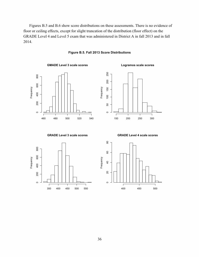
Figures B.5 and B.6 show score distributions on these assessments. There is no evidence of floor or ceiling effects, except for slight truncation of the distribution (floor effect) on the GRADE Level 4 and Level 5 exam that was administered in District A in fall 2013 and in fall 2014.
Figure B.5. Fall 2013 Score Distributions
GMADE Level 3 scale scores
Frequency
460 480 500 520 540
0200
400
600
800
Logramos scale scores
Frequency
150 200 250 300
050
100
150
200
250
GRADE Level 3 scale scores
Frequency
350 400 450 500 550
0200
400
600
800
GRADE Level 4 scale scores
Frequency
400 450 500
020
4060
80

37
Figure B.6. Fall 2014 Score Distributions
End-of-Course Grades
The five districts varied in their course grade systems. A summary of the grade systems is presented in Tables B.3 and B.4. In spring 2014, District D reported both reading and LA grades, and we computed an average across domains. By spring 2015, this changed to only a reading grade. District B did not give overall course grades, but recorded between four and five domain-specific scores for each subject in each trimester (Table B.4). To maintain interpretable cross-district comparisons, we first rescaled course grades from the final marking period from each district on a 1–5 numeric scale, equivalent to an A–F letter grade system (i.e., 1 = F, 2 = D, 3 = C, 4 = B, and 5 = A). Then, for districts with separate grades in multiple LA domains (e.g., in District D), we created an overall LA grade by averaging across those domains. Similar steps were taken in District B: For mathematics, an overall grade was created by averaging across the four mathematics domain scores; for LA, an overall grade was created by averaging across the
Scale Score
Density
0.00
0.01
0.02
0.03
0.04
480 500 520 540
GMADE scale scoresGMADE scale scores
0.000
0.005
0.010
0.015
200 250 300
Logramos scale scoresLogramos scale scores
0.000
0.005
0.010
400 450 500
GRADE Level 5 scale scoresGRADE Level 5 scale scores
0.000
0.005
0.010
400 450 500 550
GRADE Level 4 scale scoresGRADE Level 4 scale scores

38
eight reading and writing domain scores. Figures B.7 and B.8 display the resulting grade distributions for mathematics and LA in spring 2014 and in spring 2015.
Table B.3. Description of Course Grading Systems
District Grades Marking Periods Mathematics LA Reading English Writing
A A–E Quarter X X X B 1–4 Trimester X X X1 C 1–9 Quarter X X D 50–100 Semester X X1 X E A–F Quarter X X
NOTE: Table applies to SYs 2013–2014 and 2014–2015. 1 As of spring 2015, there were two changes: District B no longer had a separate writing grade, and District D no longer had an LA grade separate from reading.
Table B.4. Domains in District B’s Language Arts and Mathematics Grading Systems
Subject Description of Domains Within the Subject
Reading Reads with fluency and accuracy Understands what is read Reads a variety of material on level Overall reading effort
Writing Spelling and vocabulary Mechanics and usage Content and organization Style and voice Overall writing effort
Mathematics Demonstrates fluency/accuracy in number sense Develops and explains strategies to solve problems Understands and applies mathematical thinking Overall math effort

39
Figure B.7. Histograms of Rescaled SY 2013–2014 Mathematics Course Grades for Each District
40
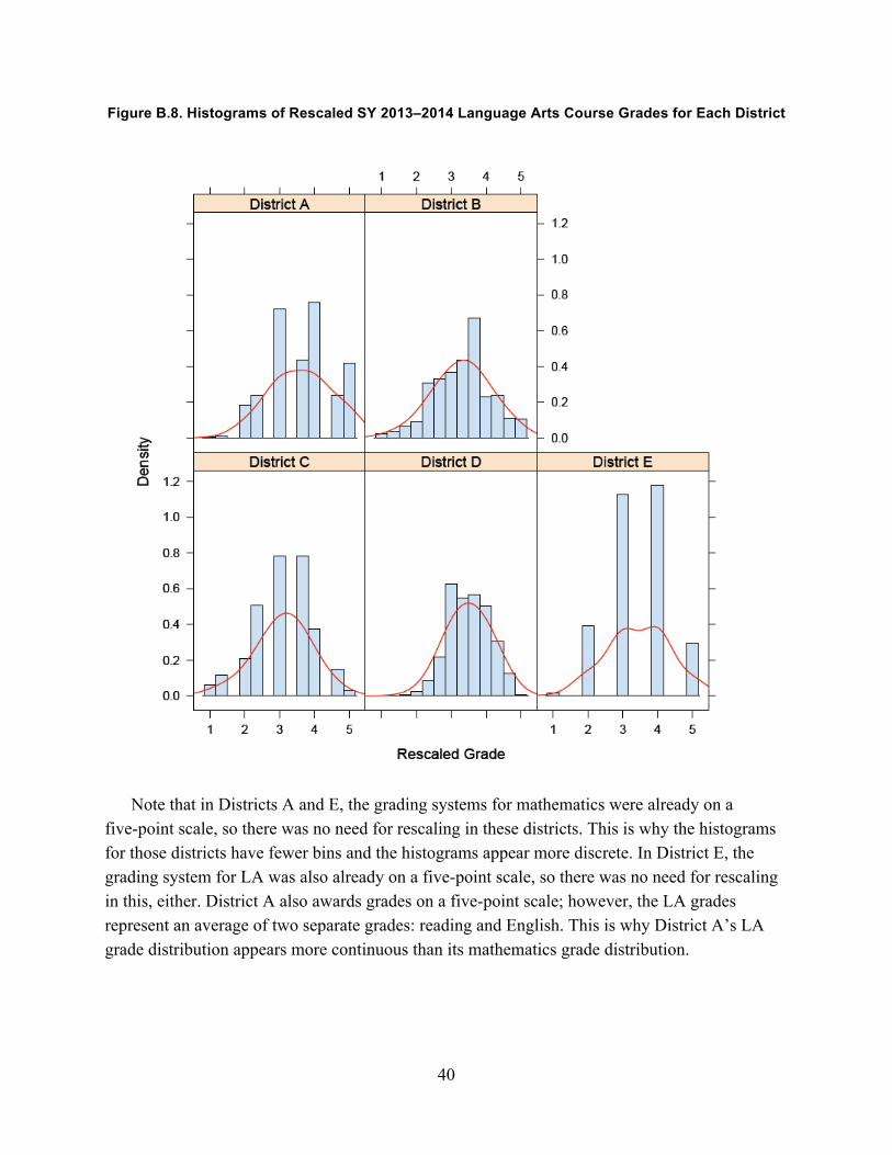
Figure B.8. Histograms of Rescaled SY 2013–2014 Language Arts Course Grades for Each District
Note that in Districts A and E, the grading systems for mathematics were already on a five-point scale, so there was no need for rescaling in these districts. This is why the histograms for those districts have fewer bins and the histograms appear more discrete. In District E, the grading system for LA was also already on a five-point scale, so there was no need for rescaling in this, either. District A also awards grades on a five-point scale; however, the LA grades represent an average of two separate grades: reading and English. This is why District A’s LA grade distribution appears more continuous than its mathematics grade distribution.

41
Figure B.9. Histograms of Rescaled SY 2014–2015 Mathematics Course Grades for Each District

42
Figure B.10. Histograms of Rescaled SY 2014–2015 Language Arts Course Grades for Each District
Suspensions
As with course grades, the five school districts had different reporting standards for suspension information. In-school suspensions and out-of-school suspensions are reported separately in Districts B and C. Districts A, D, and E report the number of days suspended for each student, but not the type of suspension nor the number of suspensions. For our analysis, we created a variable (ever suspended) to indicate whether a student had ever been suspended (either in school or out of school) during the 2013–2014 academic year or the 2014–2015 academic year. For any students who were missing all other spring outcomes (i.e., course grades, spring
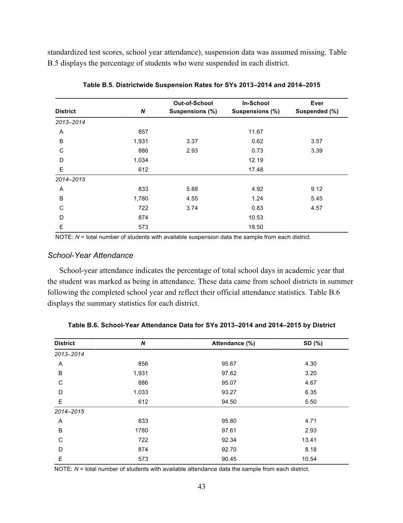
43
standardized test scores, school year attendance), suspension data was assumed missing. Table B.5 displays the percentage of students who were suspended in each district.
Table B.5. Districtwide Suspension Rates for SYs 2013–2014 and 2014–2015
District N Out-of-School
Suspensions (%) In-School
Suspensions (%) Ever
Suspended (%)
2013–2014 A 857 11.67 B 1,931 3.37 0.62 3.57 C 886 2.93 0.73 3.39 D 1,034 12.19 E 612 17.48
2014–2015 A 833 5.88 4.92 9.12 B 1,780 4.55 1.24 5.45 C 722 3.74 0.83 4.57 D 874 10.53 E 573 18.50
NOTE: N = total number of students with available suspension data the sample from each district.
School-Year Attendance
School-year attendance indicates the percentage of total school days in academic year that the student was marked as being in attendance. These data came from school districts in summer following the completed school year and reflect their official attendance statistics. Table B.6 displays the summary statistics for each district.
Table B.6. School-Year Attendance Data for SYs 2013–2014 and 2014–2015 by District
District N Attendance (%) SD (%)
2013–2014 A 856 95.67 4.30 B 1,931 97.62 3.20 C 886 95.07 4.67 D 1,033 93.27 6.35 E 612 94.50 5.50
2014–2015 A 833 95.80 4.71 B 1780 97.61 2.93 C 722 92.34 13.41 D 874 92.70 8.18 E 573 90.45 10.54
NOTE: N = total number of students with available attendance data the sample from each district.

44
Social-Emotional Outcomes Broadly, social-emotional competence refers to the ability of students to successfully interact
with other students and adults in a way that demonstrates an awareness of, and ability to manage, emotions in an age- and context-appropriate manner. To measure social and emotional well-being in the fall after the summer programs, RAND administered the Devereux Student Strengths Assessment–RAND Research Edition (DESSA-RRE) to school-year teachers who reported on the behaviors of individual study students. RAND administered the DESSA-RRE at two points: fall 2013 and fall 2014. The DESSA is a strength-based assessment that assesses only positive behaviors rather than maladaptive ones.11
The DESSA-RRE is one scale of 27 items that RAND staff selected from the original pool of 72 items on the DESSA (LeBuffe, Shapiro, and Naglieri, 2009). RAND selected these items based on their alignment with the school districts’ stated goals for their summer programming. Drawing on student data from the DESSA national standardization sample, the developers determined that the pool of 27 items has a high degree of reliability; the 27 items and the corresponding coefficient Alpha are listed in Table B.7.
RAND administered the DESSA-RRE online to a treatment student’s teacher of record beginning on the first day of the 11th week of the school year. We selected this timing because it was the first time point at which a large majority of students would have been assigned to their teacher of record for at least four weeks. (Each district had determined the teacher of record no later than the first day of the tenth week of the school year.) For each of the 27 items in the DESSA-RRE, the rater is asked to indicate on a five-point scale how often the student engaged in each behavior over the past four weeks.
The survey took approximately five minutes to complete per student, and teachers were given a $20 Amazon gift card per survey completed. Teachers were required to answer 26 of 27 items for a survey to be deemed complete. In fall 2013, we obtained responses from 84.0 percent of teachers of record and for 79.0 percent of the study students. Using district data for students who had left the district as of the time that we administered the DESSA, the effective response rate was 86.4 percent of the still-enrolled student sample. In fall 2014, we obtained responses from 77 percent of teachers of record and for 66.0 percent of the study students. Using district data for students who had left the district as of the time that we administered the DESSA, the effective response rate was 75.1 percent of the still-enrolled student sample.
With the fall 2013 DESSA-RRE results, we performed exploratory factor analyses and identified two subscales with high levels of internal consistency reliability. The items loading on each scale and the scales’ reliability are also shown in Table B.7. We generated scores for the scales by averaging responses across the relevant items for each student. To these scales we assigned the names self-regulation (for items generally about students’ ability to control their
11 Development of the DESSA was led by Paul LeBuffe, Valerie Shapiro, and Jack Naglieri at the Devereux Center for Resilient Children and made publicly available in 2009.

45
behavior and interactions) and self-motivation (for items generally about students’ academic focus and drive).
Table B.7. DESSA-RRE Social-Emotional Behavior Scales
Behavior
Overall Social-Emotional Behavior Scale
Self-Regulation
Scale
Self-Motivation
Scale
Coefficient Alpha 0.968 0.969 0.954
During the past four weeks, how often did the child…
Carry herself/himself with confidence ü ü
Keep trying when unsuccessful ü ü
Say good things about herself/himself ü ü
Compliment or congratulate someone ü ü
Show good judgment ü ü
Pay attention ü ü
Wait for her/his turn ü ü
Act comfortable in a new situation ü ü
Do things independently ü ü
Respect another person's opinion ü ü
Contribute to group efforts ü ü
Do routine tasks or chores without being reminded ü ü
Perform the steps of a task in order ü
Show creativity in completing a task ü ü
Share with others ü ü
Accept another choice when first choice was unavailable ü
Say good things about the future ü ü
Stay calm when faced with a challenge ü ü
Attract positive attention from adults ü ü
Cooperate with peers or siblings ü ü
Show care when doing a project or school work ü ü
Make a suggestion or request in a polite way ü ü
Learn from experience ü ü
Work hard on projects ü ü
Follow rules ü ü
Offer to help somebody ü ü
Adjust well when going from one setting to another ü ü

46
Student Survey Responses To understand both the control and treatment groups’ participation in any type of camp or
summer school activity, the study included a short student survey about their activities during summer 2013 and in summer 2014. At the same time that Mathematica Policy Research administered the GMADE, GRADE, and/or Logramos to students in the study at fall 2013 and fall 2014, Mathematica Policy Research also administered a four- or five-question survey to students. The survey was also translated into Spanish, and students who took the Logramos instead of the GRADE took the Spanish version of the student survey. Given the wide variety of summer programming available to students in the five school districts where the study occurred, the primary purpose of the survey was to gauge the contrast between the treatment and control group’s exposure to any type of summer programming during summer 2013 and summer 2014.
Table B.8 reports the number of students who completed the student survey and the proportions who answered each item in summer 2013. The table first summarizes the language in which students took the survey, and then the treatment and control group responses to each survey item. Table B.9 reports the same information and the slight deviations plus a new question added to the summer 2014 survey.
Table B.8. Summer 2013 Student Survey Responses
Treatment Group Respondents
Control Group Respondents
Survey Item N Percentage N Percentage Language in which student took the survey English 2,429 82.9 1,737 78.8 Spanish 500 17.1 468 21.2
At home this last summer, I read a book or a magazine Never 370 12.7 321 14.7 A few times this summer 1,563 53.6 1,159 52.9 At least once a week 986 33.8 710 32.4
This last summer, I went to camp or summer school Did not go to camp or summer school 546 18.7 1,270 57.7 Went for a few days 238 8.1 125 5.7 Went for one week 154 5.3 111 5.0 Went for a few weeks 728 24.9 253 11.5 Went for at least a month 1,256 43.0 442 20.1
I did reading and writing at my camp or summer school this last summer Did not go to camp or summer school 544 18.8 1,269 58.6 No 168 5.8 230 10.6 Yes 2,179 75.4 665 30.7
I did math at my camp or summer school this last summer Did not go to camp or summer school 545 18.8 1,272 58.7 No 185 6.4 363 16.7 Yes 2,169 74.8 533 24.6
NOTE: Not all students answered each of the four survey questions. Thus, the sum of respondents for each item is not always equal.

47
Table B.9. Summer 2014 Student Survey Responses
Treatment Group Respondents
Control Group Respondents
Survey Item N Percentage N Percentage
Language in which student took the survey English 2,130 83.1 1,558 79.4 Spanish 432 16.9 405 20.6
At home this last summer, I read a book or a magazine Never 360 14.1 269 13.7 A few times this summer 874 34.1 725 36.9 At least once a week 646 25.2 531 27.0 Every day or almost every day 681 26.6 437 22.3
This last summer, I went to camp or summer school I did not go to camp or summer school 809 31.6 1,263 64.4 Went for a few days 124 4.9 83 4.2 For one week 69 2.7 74 3.4 For two weeks 96 3.7 60 3.1 For three weeks 208 8.1 91 4.6 For at least one month 1,253 49.0 391 19.9
I did reading at my camp or summer school this last summer almost every day
Did not go to camp or summer school 787 30.8 1,219 62.5 No 283 11.1 265 13.6 Yes 1,486 58.1 466 23.9
I did math at my camp or summer school this last summer almost every day
Did not go to camp or summer school 775 30.4 1,198 61.2 No 230 9.0 361 18.5 Yes 1,545 60.6 398 20.3
Which of these things did you do every day or almost every week last summer?
Took care of a younger sibling or relative during the day 1,025 40.0 771 39.3 Went to a place like a pool, park, theme park, mall, or movie theater
1,966 76.7 1,535 78.2
Went to an educational place like a library or museum 811 31.6 572 29.1 Played with kids in my neighborhood 1,346 52.5 1,022 52.1 Stayed mostly in the house 803 31.3 697 35.5 I did not do any of these things 94 3.7 53 2.7
NOTE: Not all students answered each of the four survey questions. Thus, the sum of respondents for each item is not always equal.
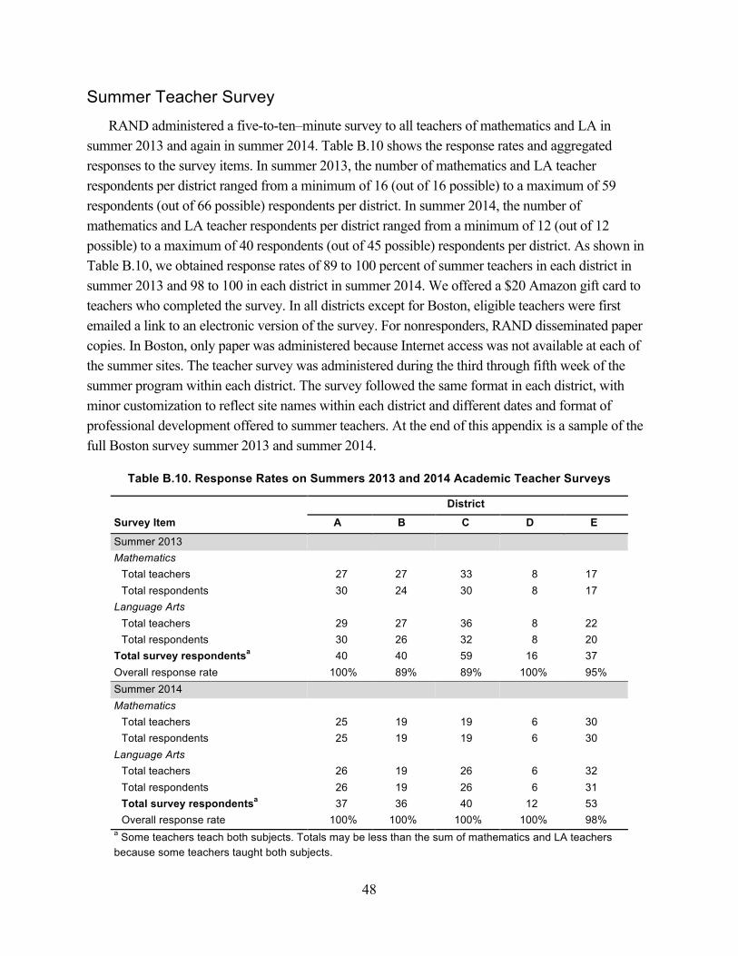
48
Summer Teacher Survey RAND administered a five-to-ten–minute survey to all teachers of mathematics and LA in
summer 2013 and again in summer 2014. Table B.10 shows the response rates and aggregated responses to the survey items. In summer 2013, the number of mathematics and LA teacher respondents per district ranged from a minimum of 16 (out of 16 possible) to a maximum of 59 respondents (out of 66 possible) respondents per district. In summer 2014, the number of mathematics and LA teacher respondents per district ranged from a minimum of 12 (out of 12 possible) to a maximum of 40 respondents (out of 45 possible) respondents per district. As shown in Table B.10, we obtained response rates of 89 to 100 percent of summer teachers in each district in summer 2013 and 98 to 100 in each district in summer 2014. We offered a $20 Amazon gift card to teachers who completed the survey. In all districts except for Boston, eligible teachers were first emailed a link to an electronic version of the survey. For nonresponders, RAND disseminated paper copies. In Boston, only paper was administered because Internet access was not available at each of the summer sites. The teacher survey was administered during the third through fifth week of the summer program within each district. The survey followed the same format in each district, with minor customization to reflect site names within each district and different dates and format of professional development offered to summer teachers. At the end of this appendix is a sample of the full Boston survey summer 2013 and summer 2014.
Table B.10. Response Rates on Summers 2013 and 2014 Academic Teacher Surveys
District
Survey Item A B C D E
Summer 2013 Mathematics
Total teachers 27 27 33 8 17 Total respondents 30 24 30 8 17
Language Arts Total teachers 29 27 36 8 22 Total respondents 30 26 32 8 20
Total survey respondentsa 40 40 59 16 37 Overall response rate 100% 89% 89% 100% 95% Summer 2014 Mathematics
Total teachers 25 19 19 6 30 Total respondents 25 19 19 6 30
Language Arts Total teachers 26 19 26 6 32 Total respondents 26 19 26 6 31 Total survey respondentsa 37 36 40 12 53 Overall response rate 100% 100% 100% 100% 98%
a Some teachers teach both subjects. Totals may be less than the sum of mathematics and LA teachers because some teachers taught both subjects.

49
Table B.11. Summer 2013 Academic Teachers’ Views of their Summer Program
Survey Item
District
A B C D E
Number of respondents (N) 40 40 59 16 37 Participation rate 100 89 89 100 95 Background
Taught in summer program in 2012 40 35 25 63 32 Worked with same students during SY 2012–2013 46 38 23 69 46
Quality and Structure of Summer Program This program is well managed and well organized 93 80 72 69 95 Support staff (e.g., camp counselors, paraprofessionals, instructional aides, tutors) provide necessary support in my classroom
90 88 81 94 86
There is a clear procedure for handling student discipline problems 80 83 88 88 81
The procedure for handling student discipline problems is effective 83 80 83 63 73
Climate and culture of summer program Administrators in this program care about students and teachers 100 100 97 100 95 Teachers listen to students when they have a problem 100 95 98 94 97 Faculty and staff make students feel cared for 100 98 100 94 100 Faculty and staff treat students with respect 100 98 100 94 100 Teachers enjoy teaching here 93 97 97 81 94 Faculty and staff remind students to be friendly and respectful to each other 98 100 100 100 97
About students in summer program Due to student misbehavior, a great deal of learning time is wasted 38 18 34 56 57
Students enjoy this summer program 95 100 83 88 95 Students solve problems without fighting or saying mean things 75 85 90 75 64 Students feel safe traveling to and being in this school 100 100 98 100 95 Students treat adults in school with respect 88 85 95 88 84 Children get into physical fights with other students at school at least once a week 8 5 7 38 35
Children are bullied and harassed by other students at least once a week 21 5 15 50 57
NOTES: Unless otherwise noted, values shown in table are the percentage of respondents who agree or strongly agree. Sources: Data from RAND’s academic teacher surveys administered in summer 2013.
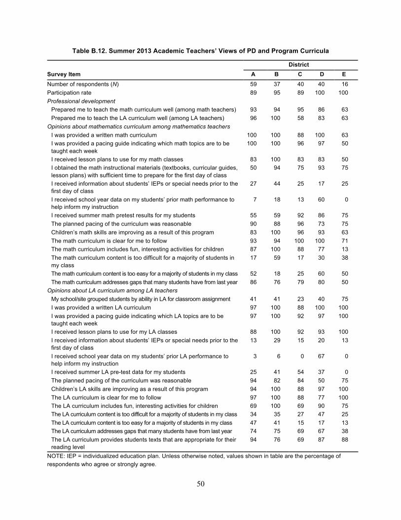
50
Table B.12. Summer 2013 Academic Teachers’ Views of PD and Program Curricula
District Survey Item A B C D E Number of respondents (N) 59 37 40 40 16 Participation rate 89 95 89 100 100 Professional development
Prepared me to teach the math curriculum well (among math teachers) 93 94 95 86 63 Prepared me to teach the LA curriculum well (among LA teachers) 96 100 58 83 63
Opinions about mathematics curriculum among mathematics teachers I was provided a written math curriculum 100 100 88 100 63 I was provided a pacing guide indicating which math topics are to be taught each week
100 100 96 97 50
I received lesson plans to use for my math classes 83 100 83 83 50 I obtained the math instructional materials (textbooks, curricular guides, lesson plans) with sufficient time to prepare for the first day of class
50 94 75 93 75
I received information about students’ IEPs or special needs prior to the first day of class
27 44 25 17 25
I received school year data on my students’ prior math performance to help inform my instruction
7 18 13 60 0
I received summer math pretest results for my students 55 59 92 86 75 The planned pacing of the curriculum was reasonable 90 88 96 73 75 Children’s math skills are improving as a result of this program 83 100 96 93 63 The math curriculum is clear for me to follow 93 94 100 100 71 The math curriculum includes fun, interesting activities for children 87 100 88 77 13 The math curriculum content is too difficult for a majority of students in my class
17 59 17 30 38
The math curriculum content is too easy for a majority of students in my class 52 18 25 60 50 The math curriculum addresses gaps that many students have from last year 86 76 79 80 50
Opinions about LA curriculum among LA teachers My school/site grouped students by ability in LA for classroom assignment 41 41 23 40 75 I was provided a written LA curriculum 97 100 88 100 100 I was provided a pacing guide indicating which LA topics are to be taught each week
97 100 92 97 100
I received lesson plans to use for my LA classes 88 100 92 93 100 I received information about students’ IEPs or special needs prior to the first day of class
13 29 15 20 13
I received school year data on my students’ prior LA performance to help inform my instruction
3 6 0 67 0
I received summer LA pre-test data for my students 25 41 54 37 0 The planned pacing of the curriculum was reasonable 94 82 84 50 75 Children’s LA skills are improving as a result of this program 94 100 88 97 100 The LA curriculum is clear for me to follow 97 100 88 77 100 The LA curriculum includes fun, interesting activities for children 69 100 69 90 75 The LA curriculum content is too difficult for a majority of students in my class 34 35 27 47 25 The LA curriculum content is too easy for a majority of students in my class 47 41 15 17 13 The LA curriculum addresses gaps that many students have from last year 74 75 69 67 38 The LA curriculum provides students texts that are appropriate for their reading level
94 76 69 87 88
NOTE: IEP = individualized education plan. Unless otherwise noted, values shown in table are the percentage of respondents who agree or strongly agree.
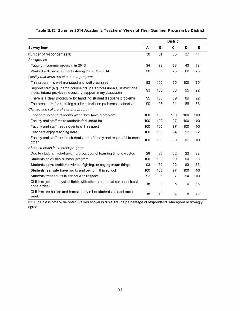
51
Table B.13. Summer 2014 Academic Teachers’ Views of Their Summer Program by District
Survey Item
District
A B C D E
Number of respondents (N) 38 51 36 37 11 Background
Taught in summer program in 2013 34 82 56 43 73 Worked with same students during SY 2013–2014 36 67 25 62 75
Quality and structure of summer program This program is well managed and well organized 93 100 85 100 75 Support staff (e.g., camp counselors, paraprofessionals, instructional aides, tutors) provides necessary support in my classroom 93 100 88 95 92
There is a clear procedure for handling student discipline problems 95 100 89 89 92 The procedure for handling student discipline problems is effective 90 98 91 86 83
Climate and culture of summer program Teachers listen to students when they have a problem 100 100 100 100 100 Faculty and staff make students feel cared for 100 100 97 100 100 Faculty and staff treat students with respect 100 100 97 100 100 Teachers enjoy teaching here 100 100 94 97 92 Faculty and staff remind students to be friendly and respectful to each other 100 100 100 97 100
About students in summer program Due to student misbehavior, a great deal of learning time is wasted 28 25 22 22 33 Students enjoy this summer program 100 100 89 94 83 Students solve problems without fighting, or saying mean things 93 89 92 83 58 Students feel safe travelling to and being in this school 100 100 97 100 100 Students treat adults in school with respect 92 98 97 94 100 Children get into physical fights with other students at school at least once a week 15 2 6 0 33
Children are bullied and harassed by other students at least once a week 15 19 14 8 42
NOTE: Unless otherwise noted, values shown in table are the percentage of respondents who agree or strongly agree.

52
Table B.14. Summer 2014 Academic Teachers’ Views of the PD and Curriculum for Their Summer Program by District
Survey Item
District
A B C D E
Number of respondents (N) 44 35 11 34 36 Professional development
Prepared me to teach the math curriculum well (among math teachers) 100 100 88 80 58 Prepared me to teach the LA curriculum well (among LA teachers) 100 93 83 72 76
Opinions about mathematics curriculum among mathematics teachers My school/site grouped students by ability in math for classroom assignment 60 26 50 29 40
By the first day of the program, I was provided a written math curriculum 100 100 100 100 84
By the first day of the program, I was provided a pacing guide indicating which math topics are to be taught each week 100 100 100 100 80
By the first day of the program, I received lesson plans to use for my math classes 100 100 100 79 84
I received information about students’ IEPs or special needs 87 42 50 11 24 I received school year data on my students’ prior math performance 30 5 67 5 8 I received summer math pre-test results for my students 77 5 0 17 67 The planned pacing of the curriculum was reasonable 100 89 83 95 76 Children’s math skills are improving as a result of this program 100 84 83 100 100 The math curriculum is clear for me to follow 100 95 100 100 76 The math curriculum includes fun, interesting activities for children 100 100 50 95 68 The math curriculum is aligned with the curriculum students received in the past school year 100 95 83 84 88
The math curriculum is aligned with the curriculum students will receive in the next school year 100 89 50 95 79
The math curriculum content is too difficult for the Level I students in my class 66 25 50 12 70
The math curriculum content is too easy for the Level I students in my class 0 0 33 0 9
The math curriculum content is too difficult for the Level II students in my class 17 0 0 13 21
About students in summer program
Due to student misbehavior, a great deal of learning time is wasted 25 28 33 22 22
Students enjoy this summer program 100 100 83 89 94
Students solve problems without fighting, or saying mean things 89 93 58 92 83
Students feel safe travelling to and being in this school 100 100 100 97 100 Students treat adults in school with respect 98 92 100 97 94 Children get into physical fights with other students at school at least once a week 2 15 33 6 0
Children are bullied and harassed by other students at least once a week 19 15 42 14 8
NOTE: Unless otherwise noted, values shown in table are the percentage of respondents who agree or strongly agree.
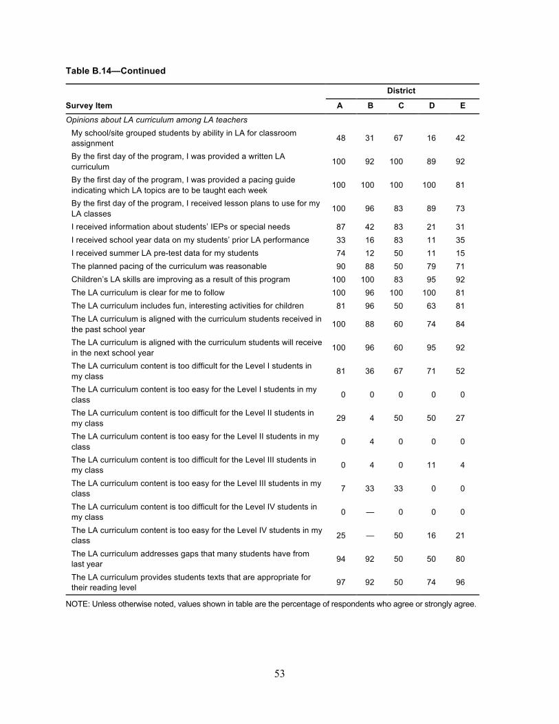
53
Table B.14—Continued
Survey Item
District
A B C D E
Opinions about LA curriculum among LA teachers My school/site grouped students by ability in LA for classroom assignment 48 31 67 16 42
By the first day of the program, I was provided a written LA curriculum 100 92 100 89 92
By the first day of the program, I was provided a pacing guide indicating which LA topics are to be taught each week 100 100 100 100 81
By the first day of the program, I received lesson plans to use for my LA classes 100 96 83 89 73
I received information about students’ IEPs or special needs 87 42 83 21 31 I received school year data on my students’ prior LA performance 33 16 83 11 35 I received summer LA pre-test data for my students 74 12 50 11 15 The planned pacing of the curriculum was reasonable 90 88 50 79 71 Children’s LA skills are improving as a result of this program 100 100 83 95 92 The LA curriculum is clear for me to follow 100 96 100 100 81 The LA curriculum includes fun, interesting activities for children 81 96 50 63 81 The LA curriculum is aligned with the curriculum students received in the past school year 100 88 60 74 84
The LA curriculum is aligned with the curriculum students will receive in the next school year 100 96 60 95 92
The LA curriculum content is too difficult for the Level I students in my class 81 36 67 71 52
The LA curriculum content is too easy for the Level I students in my class 0 0 0 0 0
The LA curriculum content is too difficult for the Level II students in my class 29 4 50 50 27
The LA curriculum content is too easy for the Level II students in my class 0 4 0 0 0
The LA curriculum content is too difficult for the Level III students in my class 0 4 0 11 4
The LA curriculum content is too easy for the Level III students in my class 7 33 33 0 0
The LA curriculum content is too difficult for the Level IV students in my class 0 — 0 0 0
The LA curriculum content is too easy for the Level IV students in my class 25 — 50 16 21
The LA curriculum addresses gaps that many students have from last year 94 92 50 50 80
The LA curriculum provides students texts that are appropriate for their reading level 97 92 50 74 96
NOTE: Unless otherwise noted, values shown in table are the percentage of respondents who agree or strongly agree.

54
Classroom Observations We conducted observations of academic and enrichment instruction in the five districts,
using the same protocol for both. To create our observation protocol, we first reviewed some widely used validated instruments (such as the Classroom Assessment Scoring System measure developed at the University of Virginia [Teachstone Training, 2016] and the Framework for Teaching developed by Charlotte Danielson [Danielson Group, 2013]). These classroom observation instruments, however, were not necessarily designed to analyze aspects of the classroom that research about summer programming indicates are the most important features linked to improvements in student achievement.
Consequently, RAND developed its own classroom observation protocol designed specifically to measure certain key aspects of our theoretical framework about how summer programs might lead to gains in student learning. The classroom observation protocol was intended to gather information on the quality of instruction, time on academic task, and other aspects of the classroom, such as opportunities for social and emotional development. We developed our own classroom observation protocol to pilot in summer 2011, designed specifically to measure certain key aspects of the theoretical framework about how summer programs might lead to gains in student learning. Based on our experience piloting the 2011 protocol, we further refined it for summer 2012 and used the revised observation protocol for both academic and enrichment classroom observations. We again refined it in summer 2013 and finally in summer 2014. The summer 2014 protocol is provided at the end of this appendix. Table B.15 indicates the number of classroom observations that RAND performed in each of the two summers.
The core domains of the classroom are described below:
• Time on task. The amount of productive time on task is positively linked to student achievement (Harnischfeger and Wiley, 1976; Lomax and Cooley, 1979; Fisher et al., 1980; Karweit and Slavin, 1982; Hawley et al., 1984; Karweit, 1985). The classroom observation protocol has a running time log of minutes spent on instruction versus noninstruction and observers categorize the types of instruction occurring throughout the class.
• Student engagement. Student engagement in tasks leads to greater academic achievement (Skinner, Kindermann, and Furrer, 2009). We therefore asked observers to rate in various ways how engaged students appeared.
• Indicators of instructional quality. At the end of each observed class period, the rater completed items relating to the safety of the instructional space, adequacy of materials, teacher/student interactions, student/student interactions, class routines, behavior management, instruction clarity, content clarity, factual accuracy of instructional content, provision of time for student independent practice, and student/student discussion of class

55
content. Raters also recorded final impressions, and described the kind of questions the teacher posed to students throughout the class.
Especially to measure time on task, RAND observers stayed in and coded the entire class, whether it was 30 or 120 minutes to code the amount of intended time spent on instruction.
Table B.15. Number of Classroom Observations Each Summer
Subject Area
District
A B C D E Total
Summer 2013 LA 57 56 46 16 36 211 LA—Writing NA NA NA NA 24 24 Walk to Intervention (LA—WTI) NA NA NA NA 47 47 Enrichment 66 71 70 11 22 240 Mathematics 34 56 38 16 34 178 Science NA NA 26 NA NA 26 Success Maker NA NA 22 NA NA 22 4go5 LA NA 4 11 4 NA 19 4go5 Math NA 3 9 4 NA 16
Total 157 190 222 51 163 783
Summer 2014 LA 46 36 32 12 37 163 Enrichment 46 53 76 15 17 207 Walk to Intervention (LA—WTI) NA NA NA NA 45 45 Mathematics 36 34 33 12 32 147 Science NA NA 28 NA NA 28 Social Studies NA NA 3 NA NA 3 iReady NA NA 14 NA NA 14
Total 128 123 186 39 132 608
Tables B.16–B.25 provide descriptive statistics derived from the summer 2014 classroom observations.

56
Table B.16. Overview of Instructional Time by District in Summer 2014
Subject Area
District
A B C D E Total
Mathematics Average number of students per classroom 8 10 13 9 10 8 Average intended class minutes 60 77 88 96 118 60 Average actual class minutes as percentage of intended (%) 100 99 100 96 93 100 Percentage of actual class minutes that were off task (%) 16 10 13 22 14 16
Percentage of actual class minutes devoted to independent practice (%) 26 31 40 28 38 26
Language arts Average number of students per classroom 10 10 12 9 9 10 Average intended class minutes 79 86 88 96 114 79 Average actual class minutes as percentage of intended (%) 109 110 98 97 95 109 Percentage of actual class minutes that were off task (%) 19 14 20 24 10 19
Percentage of actual class minutes devoted to independent practice (%) 17 49 19 35 36 17
Enrichment Average number of students per classroom 10 10 12 9 9 10 Average intended class minutes 79 86 88 96 144 79 Average actual class minutes as percentage of intended (%) 109 110 98 97 95 109 Percentage of actual class minutes that were off task (%) 19 14 20 24 10 19
Percentage of actual class minutes devoted to independent practice (%) 17 49 19 35 36 17
NOTE: Values shown in the total column are the weighted average of the classrooms RAND observed.
Table B.17. Summer 2014 Mathematics Practices That Support Student Engagement by District
Description
District
A (N = 34)
B (N = 36)
C (N = 33)
D (N = 12)
E (N = 32)
Prior to students doing independent practice, the teacher explained or wrote down what students would do or what skills they would cover during the overall session.
94 92 82 92 97
Prior to students doing independent practice, the teacher states the purpose for what they will do (i.e., why students would learn the skill in terms of real world relevance)
6 11 6 8 0
Large majority of students are on-task throughout class period 76 67 82 73 88 Teacher: (1) performs ongoing assessment throughout the whole class period by checking for students' understanding of content, and (2) addresses misunderstanding if and as they arise
59 72 24 75 56
Little to no time is wasted; pacing is efficient. The class resembles a “well-oiled machine” where a majority of students know what is expected of them and how to go about doing it throughout the whole class
53 58 52 42 69
NOTE: Values shown are the percentage of classroom observations rated yes out of total rated observations.

57
Table B.18. Summer 2014 Desirable Mathematics Classroom Practices by District
Description
District
A (N = 34)
B (N = 36)
C (N = 33)
D (N = 12)
E (N = 32)
Students respect one another 100 100 91 83 97 All or almost all students exhibited obvious signs of enthusiasm for the class throughout the class period (e.g., jumping out of seat, quickly and enthusiastically answering teacher’s questions)
3 0 12 17 3
The teacher (a) explicitly encouraged at least one student struggling with a particular task to persist at academic/ content-related tasks that were difficult for them or (b) explicitly taught students strategies to persist at tasks
9 28 39 25 41
There was a helpful adult other than the teacher in the classroom (Helpful means the adult worked directly with students, engaged in the material, or supporting students learning while they were in the room for a majority of the class time)
9 42 21 92 38
Students verbally encourage each other, are overtly friendly and supportive
15 0 9 8 3
Teacher shows explicit signs of caring and positive affect toward youth
21 19 45 25 59
Students show explicit signs they have warm, positive affect to teacher 12 8 24 8 41
Lesson is characterized by appropriately challenging, rigorous tasks that engage critical thinking skills
27 39 18 33 13
The teacher explicitly taught social skills such as respecting, listening, cooperating with, or helping others or teaching of politeness
0 0 6 0 3
NOTE: Values shown are the percentage of classroom observations rated yes out of total rated observations.
Table B.19. Summer 2014 Undesirable Mathematics Classroom Practices by District
Description
District
A (N = 34)
B (N = 36)
C (N = 33)
D (N = 12)
E (N = 32)
The teacher provided or failed to correct factually inaccurate information that would confuse students about the content/skills they were to learn
9 0 24 0 0
The explanation of the instructional content was unclear, hard to follow, incomplete, or inconsistent
15 6 21 8 6
In at least one instance, the teacher was disrespectful to students 0 0 9 8 16
There was one or more flagrant instance of student misbehavior 0 0 0 0 3
When the teacher disciplined students, the majority of the class was interrupted for a long period
12 0 3 8 6
The teacher responsible for the activity was disengaged in the classroom because of distractions by factors that were within her control
9 8 6 0 9
There were adults other than the teacher in the classroom who engaged in activities that distracted from learning (e.g., checking cell phone, interrupting the lesson, asking off-topic questions)
6 3 6 8 6
NOTE: Values shown are the percentage of classroom observations rated yes out of total rated observations.

58
Table B.20. Summer 2014 LA Practices That Support Student Engagement by District
Description
District
A (N = 37)
B (N = 36)
C (N = 32)
D (N = 12)
E (N = 46)
Prior to students doing independent practice, the teacher explained or wrote down what students would do or what skills they would cover during the overall session
100 94 88 67 96
Prior to students doing independent practice, the teacher states the purpose for what they will do (i.e., why students would learn the skill in terms of real world relevance)
0 8 6 17 4
Large majority of students are on-task throughout class period. 65 86 72 50 65 Teacher: (1) performs ongoing assessment throughout the whole class period by checking for students' understanding of content, and (2) addresses misunderstanding if and as they arise
8 58 22 58 50
Little to no time is wasted; pacing is efficient. The class resembles a “well-oiled machine” where a majority of students know what is expected of them and how to go about doing it throughout the whole class
43 83 41 25 26
NOTE: Values shown are the percentage of classroom observations rated yes out of total rated observations.
Table B.21. Summer 2014 Desirable LA Classroom Practices by District
Description
District
A (N = 37)
B (N = 36)
C (N = 32)
D (N = 12)
E (N = 46)
Students respect one another 92 100 84 75 98
All or almost all students exhibited obvious signs of enthusiasm for the class throughout the class period (e.g., jumping out of seat, quickly & enthusiastically answering teacher’s questions)
3 17 9 0 2
The teacher (a) explicitly encouraged at least one student struggling with a particular task to persist at academic/content-related tasks that were difficult for them or (b) explicitly taught students strategies to persist at tasks
27 11 16 0 17
There was a helpful adult other than the teacher in the classroom. Helpful means the adult worked directly with students, engaged in the material, or supporting students learning while they were in the room for a majority of the class time
49 11 13 100 63
Students verbally encourage each other, are overtly friendly and supportive
8 11 19 8 4
Teacher shows explicit signs of caring and positive affect toward youth
24 28 38 25 20
Students show explicit signs they have warm, positive affect to teacher 16 14 13 17 20
Lesson is characterized by appropriately challenging, rigorous tasks that engage critical thinking skills
5 25 9 0 15
The teacher explicitly taught social skills such as respecting, listening, cooperating with, or helping others or teaching of politeness
5 6 3 17 7
NOTE: Values shown are the percentage of classroom observations rated yes out of total rated observations.

59
Table B.22. Summer 2014 Undesirable LA Classroom Practices by District
Description
District
A (N = 37)
B (N = 36)
C (N = 32)
D (N = 12)
E (N = 46)
The teacher provided or failed to correct factually inaccurate information that would confuse students about the content/skills they were to learn
0 3 13 17 0
The explanation of the instructional content was unclear, hard to follow, incomplete, or inconsistent
11 0 3 25 4
In at least one instance, the teacher was disrespectful to students
22 0 0 17 0
There was one or more flagrant instance of student misbehavior 5 0 0 0 2
When the teacher disciplined students, the majority of the class was interrupted for a long period
16 19 3 0 2
The teacher responsible for the activity was disengaged in the classroom because of distractions by factors that were within her control
22 0 9 0 2
There were adults other than the teacher in the classroom who engaged in activities that distracted from learning (e.g. checking cell phone, interrupting the lesson, asking off-topic questions)
11 8 0 0 4
NOTE: Values shown are the percentage of classroom observations rated yes out of total rated observations.
Table B.23. Summer 2014 Enrichment Practices That Support Student Engagement by District
Description
District
A (N = 46)
B (N = 15)
C (N = 76)
D (N = 53)
E (N = 17)
Prior to students doing independent practice, the teacher explained or wrote down what students would do or what skills they would cover during the overall session
82 67 70 85 100
Prior to students doing independent practice, the teacher states the purpose for what they will do (i.e., why students would learn the skill in terms of real world relevance)
4 0 7 4 0
Large majority of students are on task throughout class period 84 73 89 70 82
Teacher: (1) performs ongoing assessment throughout the whole class period by checking for students’ understanding of content, and (2) addresses misunderstanding if and as they arise
96 100 86 60 94
Little to no time is wasted; pacing is efficient. The class resembles a “well-oiled machine” where a majority of students know what is expected of them and how to go about doing it throughout the whole class
45 47 53 32 71
NOTE: Values shown are the percentage of classroom observations rated yes out of total rated observations.

60
Table B.24. Summer 2014 Desirable Enrichment Classroom Practices by District
Description
District
A (N = 46)
B (N = 15)
C (N = 76)
D (N = 53)
E (N = 17)
Students respect one another 96 73 96 89 94
All or almost all students exhibited obvious signs of enthusiasm for the class throughout the class period (e.g., jumping out of seat, quickly and enthusiastically answering teacher’s questions)
65 40 55 36 53
The teacher (a) explicitly encouraged at least one student struggling with a particular task to persist at academic/content-related tasks that were difficult for them or (b) explicitly taught students strategies to persist at tasks
9 20 28 4 29
There was a helpful adult other than the teacher in the classroom. Helpful means the adult worked directly with students, engaged in the material, or supporting students learning while they were in the room for a majority of the class time
85 100 26 8 71
Students verbally encourage each other, are overtly friendly and supportive
13 13 25 9 41
Teacher shows explicit signs of caring and positive affect toward youth
22 27 36 9 41
Students show explicit signs that they have warm, positive affect to teacher
22 27 22 13 41
The teacher explicitly taught social skills such as respecting, listening, cooperating with, or helping others or teaching of politeness
11 13 5 11 6
NOTE: Values shown are the percentage of classroom observations rated yes out of total rated observations.
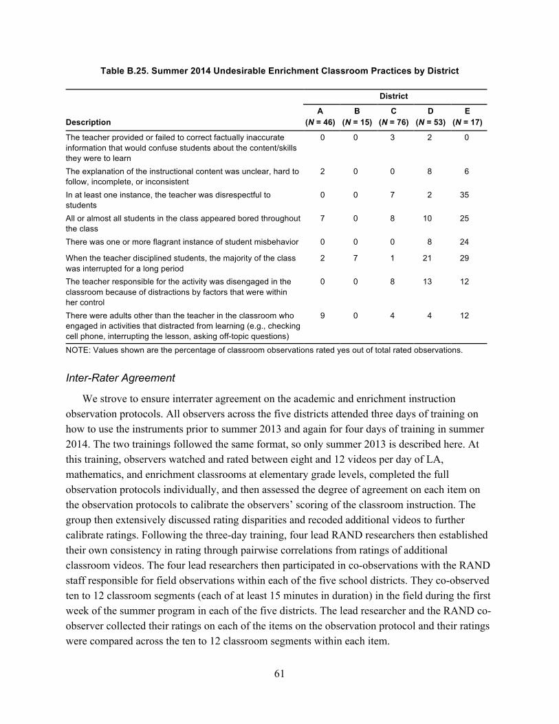
61
Table B.25. Summer 2014 Undesirable Enrichment Classroom Practices by District
Description
District
A (N = 46)
B (N = 15)
C (N = 76)
D (N = 53)
E (N = 17)
The teacher provided or failed to correct factually inaccurate information that would confuse students about the content/skills they were to learn
0 0 3 2 0
The explanation of the instructional content was unclear, hard to follow, incomplete, or inconsistent
2 0 0 8 6
In at least one instance, the teacher was disrespectful to students
0 0 7 2 35
All or almost all students in the class appeared bored throughout the class
7 0 8 10 25
There was one or more flagrant instance of student misbehavior 0 0 0 8 24
When the teacher disciplined students, the majority of the class was interrupted for a long period
2 7 1 21 29
The teacher responsible for the activity was disengaged in the classroom because of distractions by factors that were within her control
0 0 8 13 12
There were adults other than the teacher in the classroom who engaged in activities that distracted from learning (e.g., checking cell phone, interrupting the lesson, asking off-topic questions)
9 0 4 4 12
NOTE: Values shown are the percentage of classroom observations rated yes out of total rated observations.
Inter-Rater Agreement
We strove to ensure interrater agreement on the academic and enrichment instruction observation protocols. All observers across the five districts attended three days of training on how to use the instruments prior to summer 2013 and again for four days of training in summer 2014. The two trainings followed the same format, so only summer 2013 is described here. At this training, observers watched and rated between eight and 12 videos per day of LA, mathematics, and enrichment classrooms at elementary grade levels, completed the full observation protocols individually, and then assessed the degree of agreement on each item on the observation protocols to calibrate the observers’ scoring of the classroom instruction. The group then extensively discussed rating disparities and recoded additional videos to further calibrate ratings. Following the three-day training, four lead RAND researchers then established their own consistency in rating through pairwise correlations from ratings of additional classroom videos. The four lead researchers then participated in co-observations with the RAND staff responsible for field observations within each of the five school districts. They co-observed ten to 12 classroom segments (each of at least 15 minutes in duration) in the field during the first week of the summer program in each of the five districts. The lead researcher and the RAND co-observer collected their ratings on each of the items on the observation protocol and their ratings were compared across the ten to 12 classroom segments within each item.

62
During summer 2013, RAND observed a total of 783 classroom sessions, and during summer 2014, RAND observed a total of 608 classroom sessions. Although this is a substantial number of observations, they represent only about 10 percent of all instruction in LA and mathematics occurring in each summer. In so doing, RAND followed each classroom cohort for one entire day. For example, if a summer site had a red group with 12 students, a green group with 11 students, and a yellow group with 13 students, RAND visited the site for three full days, observing the red group on the first visit, the green group during the second visit, and the yellow group during the third. (Table B.15 displays the number of observations and subjects.) For each classroom observed, the RAND staff person observed the entire class session from start to finish, coding a minute-by-minute time log during the class session, and then, at the end of class, answered 24 yes/no items plus six open-ended response items.
Daily Site Observation
As of summer 2014, at the end of each day in which an observer followed a cohort of students through the day, the RAND observer would then fill out a short online survey with the yes-or-no questions shown in Table B.26. This survey was completed in addition to the classroom observations and interviews that the observer conducted that day. The observers were trained on this instrument during the weeklong training in spring 2014.The items were used to develop a site-level climate index for summer 2014 only. Table B.26 reports the average ratings on each item on the five-point scale.
Table B.26. RAND Daily Site Observation by District
Survey Item
District
A B C D E
Number of site observations within the district (N) 35 33 39 13 34 Adults at the site address student behavior consistently and appropriately when misbehavior occurs
3.7 4.1 3.2 2.9 3.4
Almost none or no student misbehavior at this site 3.9 3.9 3.0 2.7 3.8 Site is well organized 3.6 4.1 3.3 2.8 3.3 Students appeared to have enjoyable day 4.0 4.1 3.3 3.6 3.3 Staff are overtly friendly toward students 3.5 4.4 3.4 3.5 3.6 Students are overtly friendly toward and supportive of one another 3.5 3.5 3.1 2.9 3.4
NOTE: Unless otherwise noted, values shown are average ratings on a 1–5 scale.
Summer Student Attendance Given known inaccuracies in the summer 2012 data collection, RAND collected and audited
each week of the five- to six-week summer program student-level daily attendance data from each of the five school districts in both subsequent summers (2013 and 2014). These checks were to ensure that control group students were not attending the summer program and to ensure that

63
attendance data was being routinely entered. We further checked for suspicious patterns, such as 100-percent attendance or absence on a given day. We used these checks to communicate with district leaders to fix software glitches and remind site leaders to submit daily or weekly attendance records (depending on the district). In one district, RAND also collected paper copies of the attendance logs to cross-check them later with that district’s electronic attendance records.
Summer Program Costs To assess the revenue and monetary costs of implementing a summer program, in fall 2014,
we collected data about the prior full year of costs, including the preparation for and the execution of the summer 2014 program. We applied a cost-ingredient approach, where we created a customized spreadsheet for each district that identified all of the known cost ingredients for the given summer program. For example, we included curriculum coordinators for districts that had hired them to write the summer reading curriculum. After developing the spreadsheets, we held calls in spring 2013 with each of the relevant sources of cost data (e.g., summer program directors, facilities services directors, food service coordinators, transportation coordinators, and—in some cases—representatives from community-based organizations [CBOs]) to preview the data request, set deadlines, and ensure the cost categories were collectable. A sample spreadsheet is included at the end of this appendix.
The data request covered the revenue sources, the number of staff positions and corresponding salaries, and line item costs for the various components of each summer program. In cases where personnel split responsibilities between the summer program and other activities, they were asked to prorate their salaries based on the percentage of time spent on the summer program. They were also asked to denote which costs were paid for out of the summer budget and which were in-kind contributions from the district. Where possible, the cost data were validated against other sources, including budgets submitted by the districts to The Wallace Foundation, publicly available salary schedules, and reimbursement rates for the federal meals program. When necessary, we used email and phone correspondence to clarify and refine the cost data and correct discrepancies.
Cost Data Collection and Cleaning
Cost data were gathered from the five participating summer programs after identifying key personnel mentioned above. Beginning in November 2014, the relevant personnel were sent a template spreadsheet that requested cost data broken out into various categories. As shown in Figure 2.5 of the main report, costs were categorized as district and site management, curriculum, enrichment, academics, food, transportation, and professional development. Table B.27 shows how we categorized each line-item cost. Not all districts reported values for each line item.

64
Table B.27. Line Item Expenses Included in Each of the Six Cost Categories
Cost Category Line-Item Costs District and site management
Curriculum
Enrichment
Academics
Food
Student transportation
Professional development
Program coordinator Summer learning director Data manager* Director of operations, student support services Evaluation staff Information technology staff* Accounts payable clerk* Legal clerk* Interns Office supplies/materials District administrator travel to sites Marketing of summer program Mileage reimbursement Fingerprinting Printing Nurses and nurse supplies Custodial staff and supplies Security personnel Site managers/administrators Behavioral coaches Utilities* Curriculum writers and coaches Curricular materials Classroom materials CBO enrichment providers/partners contracts CBO partner instructors CBO partner administrative staff CBO partner curricular materials/development Evaluation Other classroom materials District-employed music/art/special resource teachers District-employed physical education teachers Field trips Scholastic Book Fair District-employed regular classroom teachers District-employed ESOL teachers District-employed special education District-employed teacher assistants Interns District-Employed Paraeducators Substitute teachers Food service staff Food service coordinator Food Snacks Transportation coordinator and routing staff Transportation contract (bus, driver, garage, maintenance) Professional development programming for teachers Professional development days for teachers
NOTE: * In-kind contributions from the district, which were not paid for out of the summer budget.

65
Our goal was to produce estimates that reflect the cost of sustaining a district-run, voluntary summer program offered to multiple grade levels. Over the course of the analysis, we had to make a number of decisions on which costs to include, how to categorize costs, and how to resolve ambiguities in the data. The list below summarizes the assumptions and decisions made in our cost analysis:
• In cases where personnel split responsibilities between the summer program and otheractivities, they were asked to prorate their salaries based on the percentage of time spenton the summer program.
• Costs that were strictly related to the study were excluded. This included travel to TheWallace Professional Learning Community conference, as well as incentives that weretargeted at boosting enrollment of treatment group students for the study.
• Districts were asked to denote which costs were paid for out of the summer budget andwhich were in-kind contributions from the district (e.g., data managers or informationtechnology personnel who supported the summer program but were not paid for out ofthe summer budget). Generally, in-kind costs were excluded from the cost estimates. Oneexception was a district that used assistant principals, who were on a 12-month contractand were therefore not paid out of the summer budget, as site leaders for the summerprogram. Because site leaders are a core element of a summer program, we include therelevant portion of those assistant principals’ salaries.
• Generally CBO services for enrichment activities were provided under fixed-pricecontracts, which may include organizational overhead or administrative costs. In mostcases, the costs of CBO services were entirely attributed to the enrichment category(Figure 2.5 in the main report). However, in one district, the CBO played an active role inthe overall program administration. In this case, after reviewing the roles andresponsibilities of each of the CBO personnel, those that were deemed part of the generalprogram administration were moved to the district and site management category, whilethose that were focused on enrichment services were included in the enrichment category.A line-item cost for administrative overhead for the CBO was also categorized underdistrict and site management.
• When calculating the cost per filled seat, we used the summer program attendance ratefor the full program (i.e., all grade levels) when available. In cases when the full programattendance was not available, we used the attendance rate for the treatment-group cohort,which was collected as part of the study.

66
Student Summer Activities Questionnaire (Fall 2014)

67
Summer 2014 Academic Teacher Survey We use the survey customized for Pittsburgh as our sample. We have intentionally omitted
the first question.

68

69
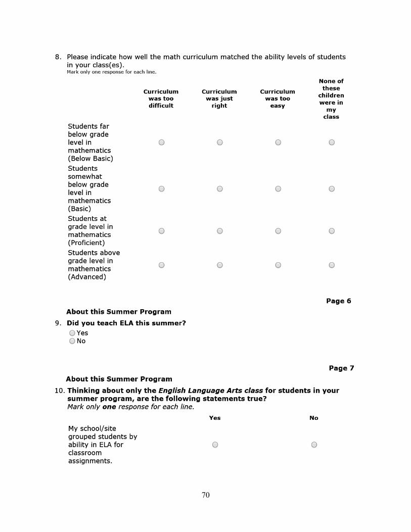
70

71

72

73
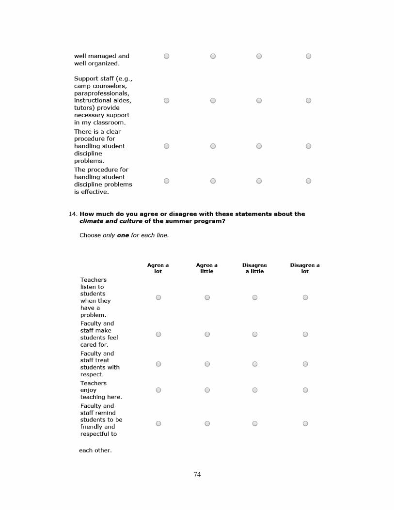
74

75

76

77
Summer 2014 Classroom Observation Protocols
Overview

78
Academic Class Segments
NOTE: Duration: Minute value is automatically calculated by the time entries.

79
Directions: Start a new row for each new activity. Segments are at least 60 seconds long. Your time log should begin when a majority of students are in the room, regardless of whether the teacher has launched the lesson. The log should end when the majority of students leave the room. You should watch and record the entire class period.
Time begin:Time of the start of the class and subsequent class segments is needed to calculate actual time, time on and off task, and time of independent practice. Start a new row for each new activity. Segments must be at least 60 seconds long to initiate new row. Your time log should begin when a majority of students are in the room, regardless of whether the teacher has launched the lesson.
Description:I indicates that majority of students are engaged in an instructional activity.NI indicates a majority of students not engaged in an subject-‐related instructional activity for more than 60seconds, e.g., off-‐topic conversation, class started late or ended early, transition to the next activity, teacher involved in management activities, break in class. End indicates the end of the class period.
Sub-‐codes for non-‐instruction: Teacher sets out classroom/behavior rules (R). Includes activities like teacher explaining what good behavior means in this classroom and what she expects. It does not include "get in a line" or disciplinary time , which should be coded as T.Teacher-‐ initiated interruption (T) includes administrative activities such as teacher taking attendance, passing out materials, or moving desks, transitions between class activities, teacher addressing behavior, bathroom breaks, and snack breaks; Externally-‐initiated interruption (E) principal visit or loudspeaker announcement that stops teaching, fire-‐drill, or other unscheduled interruption out of teacher's control; Pause for scheduled break in class (P), for example lunch and recess occur between part 1 and 2 of an ELA lesson. This code allows us to pause the class segments timer.
Teacher modeled what students will do (I do): Teacher explicitly models what students will do. The teacher is delivering direct instruction that builds students understanding of ELA or mathematics. Teacher models step-‐by-‐step how students will do an academic task; there is little to no student participation during the teacher modeling.
Whole-‐group Guided Practice (We do): Yes indicates that the teacher facilitates in a structured or semi-‐structured way a whole group activity where the kids demonstrate or practice a skill as a whole group. Some students might practice or demonstrate a skill or strategy in front of the entire class, share their thinking about how or why they used the skill or strategy, and received feedback. Although only some students may answers or solutions aloud, all students have an opportunity to hear how to practice the targeted skill or strategy. All students might complete portions of an activity before reviewing the concepts as a class. Guided practice sets students up to successfully complete an application activity of the skill or strategy independently. Guided practice provides teachers an opportunity to understand if students have a misconception and where the misconception or misunderstanding may be occurring.I-‐R-‐E that asks only for the correct answer and does not require students to share their thinking or approach to completing the activity is not guided practice. A student who doesn't understand concept would benefit from seeing guided practice. Teacher question: What is the vocabulary word that means low cost? Student response: Inexpensive. What is 3+5? Or what is the solution to number 5? Does not count as guided practice. Reviewing solutions or answers without conceptual discussion does not count as guided practice.
Example of whole group guided practice in mathematics: What is the first step to solving the problem? How do you know? Is there another way we would have started this problem? What do we do next? Teacher facilitates a discussion where students solve a fraction equation aloud is an example of whole group guided practice. All students might write the steps on worksheets while they solve the problem or steps might be written on the board as a reference for students.
Example of whole group guided practice in ELA: Teacher reads a passage aloud and asks students to summarize the passage. Student shares summary and teacher asks questions of other students about why details were excluded from the summary and others were included in the summary. Asks students for other variations of the summary. Teacher may distribute four different passages to students. Asks students to develop a summary for the passage as a team, present the summary, and explain rationale for what was included or excluded in the summary. As the independent practice, students would summarize passages in their independent reading books or a worksheet for a sustained period of time. In a mini-‐lesson, students may be asked to edit the passage from the teacher's writer's notebook. Students and teachers provide feedback and discuss editing choices before students edit text passages independently.
Small-‐group Guided Practice (We do): Yes indicates that the teacher facilitates in a structured or semi-‐structured way an activity that provides insights into the existence of misconceptions in students and where the misconception or misunderstanding may occur. Guided practice sets the small group of students up to successfully complete an application activity of the skill or strategy independently. The teacher could also reteach a mini lesson to a small group of students if the teacher determines only a group experiences a misconception or misunderstanding that prevents successful independent practice.
Independent Practice (You do): Yes indicates that students have independent practice opportunity with subject content for that time segmentIndependent Practice (YES if it occurs): Students have independent practice, whether in small groups or independent work. Do not count pair and shares or brief (< 2 min) activities. Students completes activities without consistent support from the teacher. E.g., reading a book and filling out a worksheet.
Duration:Minute value is automatically calculated by the time entries.

80
Enrichment Class Segments
NOTE: When kids start an activity on their own or do an activity, start a new segment.

81
Evidence of Classroom Practices

82
Evidence of Summer School Climate
19)
Yes/No Notes to observer
a.
RESPECT. Students respect one another. They refrain from derogatory comments or actions about an individual person and the work s/he is doing; if disagreements occur, they are handled constructively. Low bar
b.FRIENDLY. Students verbally encourage each other, are overtly friendly and supportive. High bar
c.
LIKE_TEACHER. Students show explicit signs that they have warm, positive affect to teacher (not just respect for teachers). For example, throughout the class they may smile at teacher, laugh with them, and/or share good-‐natured jokes. High bar
d.
LIKE_STUDENTS. Teacher shows explicit signs of positive affect toward youth. Mark no if teacher is simply respectful toward students. Teacher tone is warm and caring. He or she uses positive language, smiles, laughs, or shares good-‐natured jokes throughout class. If no verbal interaction is necessary, teacher demonstrates a positive and caring affect toward youth. High bar
e.
DISRESPECTFUL. In at least one instance, the teacher was disrespectful to students. This includes yelling at one or more students, intimidating or being rude or dismissive to students, using physical aggression, intentionally humiliating or ignoring a student, using discriminatory acts or derogatory language to students.
f.
MISBEHAVIOR. There was one or more flagrant instance of student misbehavior. This includes a physical fight or persistent bullying or persistent use of discriminatory or derogatory language.
g.
PERSIST. The teacher (a) explicitly encouraged at least one student struggling with a particular tasks to persist at academic/content-‐related tasks that were difficult for them (e.g., exhortations to keep trying, you know you can do it, helping students stick with rather than quit a task, to stretch to a higher level than the one student currently performs at), or (b) explicitly taught students strategies to persist at tasks.
h.
SOCIALSKILLS. The teacher explicitly taught social skills such as respecting, listening, cooperating with, or helping others or teaching of politeness. Do not check if these skills were implicitly involved.
i.
TDISENGAGED. The teacher responsible for the activity was disengaged in the classroom because of an apathetic, flat affect, or by going through the motions, or exerting extremely low effort (e.g., reading off script without deviation) or because of distractions by factors that were within her control (i.e., a teacher stopping by to have a conversation about the weekend, the teacher checking his/her cell phone, texting, or taking or making a personal call that was not related to an emergency, personal chat with co-‐teacher or paraprofessional while students are working).
J.
BORED. All or almost all students in the class appeared bored throughout the class. Boredom characterized the class period, even if students complied with teachers' requests. NA for academics.
Evidence of summer school climate. For each statement below, enter "y" if you see the practice, and "n" if you did not see the practice or if it does not apply. Skip this table if you are observing a class with no intended instruction--e.g., recess, only independent reading, only indep. writing, or SuccessMaker in Duval.

83
Overall Reactions
20) LEARNED. Based on evidence of student demonstrations, what did students learn?
21) BARRIERS. What, if any, were the main impediments or barriers to learning in this class? Note, please give examples of factual inaccuracies or shortage of materials.
22) RATING. Rate this class terrible, mixed, good, or outstanding.
OVERALL REACTIONS. Type in white cells below your overall impressions. Row height will expand as you type.

84
Data Request Form for Summer 2014 District-Level Costs We present the form customized for Boston as our sample.
Complete Set of Revenue Sources Dollar amount
Wallace Foundation funds $Title I $SIG or ARRA $General funds $Federal meals $21CCLC $IDEA-B $City funds $Title II $Other: $Other: $
1. Complete Set of Expenditures Related to District-Level Administration of Summer Learning Program (BPS & BASB)
We want to know all the revenues sources and expenditures from the period September 2013-August 2014 to the district and to its partners associated with running only the Summer Learning Project - national study sites. Please prorate any cross-program shared expenditures as necessary so they relate only to the Summer Learning Program.
List amounts for each type of revenue source for the Summer Learning Program. The list below is a sample of potential resource types. When adding up total revenues, think about the costs of planning the summer program, administering the actual program, and the cost for closing out the program.
Please list all of the expenditures by BPS & BASP and its partners in carrying out the Boston Summer Learning Program for national study sites. Examples below. Please include all staff who float across schools (e.g., coaches, nurses), district employees who work on summer, and CBO staff that work on summer in a cross-site administrative capacity. Staff that work in a single school/site during the should be listed in Section 2 school-level expenditures below.

85
1A. District administrators who worked on the Summer Program and the time they spent doing so Dollar amount
Paid out of summer
budget (Y/N)?
Number of staff in this category
Ex: curriculum designer each @ 10% FTE list 10% of salary + benefits for BOTH curric designers here Y 2BPS Summer Learning Coordinator (Ariana) $Chief Academic Officer $Director of Extended Learning Services (Melissa) $Katy Hogue (Data) $Curriculum Specialists (Kerri & Chris) $ 2BPS Coaches $ 6Denise Jordan? (payroll assistance) $Other: $Other: $
Sum of Section 1A expenditures for district-level staff
If it is too sensitive to list individuals' salary plus benefits line by line immediately above, please fill in column B as shown in the examples for each staff person but leave their corresponding cells in column C blank and only report sum of these expenditures
1B. Other district-level Expenditures here incurred by the district (BPS & BASB) Dollar amount
Paid out of summer
budget (Y/N)?Food (breakfasts, lunch, snacks, water, food safety training, delivery) $Curricular materials & Support from Curriculum Companies (storage and distribution, reordering/refreshing, Voyager, Coach training and PD etc) $Consulting Expenditures $
BASB & BPS Office supplies & materials (printer, mailings, phone, paper, scanner, computers, etc.) $Adults' travel to meetings during summer 2014 for coordination/oversight $BASB/BPS incurred costs for training( room rental, materials, social-emotional training expenditures, etc.) $Marketing and Communication of summer programming (engagement grants, parent mailers, translations) $District PD (travel to Wallace PLC, NSLA expenditures, etc.) $
Evaluation expenditures (e.g., district evaluation services to analyse pre- post- district assessments) $PEAR Workshops $Planning Grant $Indirect costs not captured above $Per-Pupil Payments to non-profit partners ($1,350 max payment per student) $Control Group Scholarships ($500 per kid) $Other: $Other: $Sum of Section 1B expenditures for other district-level costs $

86
1C. BASB employees who worked on Summer Learning Program National Study Sites in a coordinating capacity across sites within the district Dollar amount
Paid out of summer
budget (Y/N)?Ex: Project manager at partner agency A @ 60% FTE $ YProject Manager of Boston After School & Beyond $Project Assistant (Alissa, Erika) $BASB Executive Director (Chris) $Project Coordinator $Other: $Other: $
Sum of Section 1C. Expenditures
If it is too sensitive to list individuals' salary plus benefits line by line immediately above, please fill in column B as shown in the examples for each staff person but leave their corresponding cells in column C blank and only report sum of these employees' costs here.
2. Complete Set of Expenditures Related to Summer Sites (BPS and BASB expenditures) Dollar amount
Paid out of summer
budget (Y/N)?
Number of staff in this category
School administrator salaries & benefits & taxes (Site Coordinators) $BPS regular classroom teachers salaries, benefits, taxes $BPS Paraeducators salaries, benefits, and taxes $Substitute teachers salaries, benefits, taxes $Engagement Coordinators salaries', benefits', taxes' $Other: $Other: $
Please compile both BASB & BPS expenditures at the school level. Please add up the expenditures for all the relevant summer sites here; we do not need expenditures broken out site-by-site.

87
Summer 2014 Daily Site Observation Protocol
The Boston form is our sample.

88

89

90
Appendix C: Recent Studies on Summer Learning
Making Summer Count: How Summer Programs Can Boost Children's Learning, published in 2011, synthesized the existing research base on summer learning loss and summer learning program effectiveness (McCombs et al., 2011). That synthesis influenced the research questions and programs addressed in this study. Since 2011, there have been several new evaluations of summer programs and trends in student achievement over the summer months. This appendix provides an update on this research to better understand what happens to student learning during the summer and how summer affects learning trajectories throughout the year.
Summer Learning Loss
Since the release of the influential Coleman report (Coleman et al., 1966), there has been an increased appreciation of the influence of students’ out-of-school time on achievement and educational attainment and the role these influences play in the development of persistent racial and socioeconomic achievement and attainment gaps. Even before students enter kindergarten, substantial achievement gaps exist along racial and socioeconomic lines (Reardon, Robinson-Cimpian, and Weathers, 2015).
Once enrolled in school, students’ out of school experiences continue to affect their educational outcomes. For example, absences from school because of illness, truancy, and weather, among other resaons, have a negative impact on student achievement, and the negative effect is even greater for low-income students (Marcotte and Hemelt, 2008; Ready, 2010; Gottfried, 2009, 2011; Gershenson, Jacknowitz, and Brannegan, 2015). Given the negative impact of absenteeism on students’ achievement, it is reasonable to ask whether students’ summer vacation, a time most often spent away from school and that makes up roughly one-quarter of the calendar year, also affects student achievement and persistent achievement gaps.
To date, the dominant understanding of student learning over the summer derives from a meta-analysis of 13 studies from 1975 to 1995. Cooper et al. (1996) found that students lost mathematics and reading knowledge over the summer, although the loss in mathematics knowledge was generally greater than in reading. This evidence also suggested losses were larger for low-income students and for all students in upper elementary and middle school grades. However, the studies in this meta-analysis are dated.12 Schools operate in a different policy environment now, and arguably that environment is more focused on enhancing student outcomes. The changed policy environment merits revisiting this research.
12 For example, the two most commonly cited studies are from the 1970s and 1980s. The first analyzed data from 42 schools in Atlanta in the early 1970s (Heyns, 1979). The second analyzed data from 750 students in Baltimore in the 1980s (Entwisle and Alexander, 1990, 1992; Entwisle, Alexander, and Olson, 2001; Alexander, Entwisle, and Olson, 2007).

91
Over the past decade, a few data sources have allowed researchers to extend our understanding of the role of summer break in student achievement and the development of persistent race and income achievement gaps. These studies either take advantage of seasonal testing in the Early Childhood Longitudinal Study Kindergarten (ECLS-K) class or the Northwestern Evaluation Association (NWEA) Measures of Academic Progress assessment, or they examine specific summer interventions.
Throughout the main report, we cite relevant current literature on summer learning loss and summer program effectiveness. While these reflect our current understanding of summer learning loss and provide important context for the current study, it is also important to acknowledge the ways in which the summer learning loss literature of the past 20 years is limited.
Summer learning loss literature has not kept pace with other research topics, such as school choice or accountability, partly because of the common practice of testing students only once during the school year. Although the ECLS-K data set includes a rich description of student and family characteristics, including summer activities, it only enables measurement of achievement over one summer for one nationally representative cohort of students—kindergarten and first grade in 2001.
The NWEA data set contains more recent test scores from nonrandom samples of students across the 50 states, but it too suffers from limitations. In most cases, the research using NWEA data does not include student socioeconomic descriptors; therefore, NWEA studies cannot evaluate the impact of student-level poverty on students’ summer learning loss as other studies have done. Further, the NWEA data do not contain school calendar information, which prevents researchers from knowing how much school time elapses after spring and before fall testing.
Researchers also differ in preferred methods of measuring students’ summer learning and its relationship with socioeconomic status. For example, while some include linear predictors for the relationship between summer learning and socioeconomic status, others model the relationship more flexibly. We think the flexible specification better captures the true relationship between poverty and summer learning, where the key differences are likely between students at the tails of the socioeconomic distribution (e.g., Reardon’s [2011] work on the widening achievement gap between students in the 10th and 90th percentiles in the income distribution).
Related to the lack of school calendar information in the NWEA data, researchers also differ in whether they adjust for the timing of fall and spring assessments. Schools do not typically assess students on the first and last day of school. As such, simply measuring the gap between two test points usually conflates school year and summer time periods. Most ECLS-K studies separate the amount of time students have spent in schools and summer breaks between testing periods using both the test administration date and school calendar information. The only publications on summer learning using NWEA data and accounting for test timing are forthcoming or working papers (Von Hippel, Hamrock, and Kumar, 2016; Atteberry, McEachin, and Bloodworth, forthcoming). Atteberry, McEachin, and Bloodworth follow Quinn’s (2014)

92
method of preprocessing the data to project students’ learning to what it would have been at the start and end of the school year, and then use standard growth model methods. Von Hippel, Hamrock, and Kumar (2016) estimated seasonal learning growth models that use school calendar data to separate school year learning from summer learning. Other NWEA studies (e.g., Rambo-Hernandez and McCoach, 2015) do not have access to school calendar data.
Finally, researchers also differ in how they estimate students’ growth trajectories over time. The common method in ECLS-K studies uses four assessments from fall of kindergarten to the spring of first grade to fit multilevel growth models (Downey, Von Hippel, and Broh, 2004; McCoach et al., 2006; Benson and Borman, 2010; Ready, 2010; Von Hippel, Hamrock, and Kumar, 2016). This data set and approach not only allow researchers to estimate the amount of summer learning (gain or loss), and how this varies by student demographics, they also allow researchers to compare how summer learning rates compare with school year learning in kindergarten and first grade. Hayes and Gershenson (2014) and Burkham et al. (2004) take a different approach, however, and only estimate students’ summer learning between the spring of kindergarten and the fall of first grade. In their analyses, they do attempt to back-out school year learning rates from the time between the administration of the spring kindergarten assessment and the end of the school year, and the start of first grade in the fall and the administration of the first-grade assessment. Although this is a plausible method to measure summer learning, it produces counterintuitive findings: Students’ summer learning rates are not only positive but also larger than school-year learning during kindergarten. Researchers using a growth model over all four assessments do not find this pattern (Downey, Von Hippel, and Broh, 2004; McCoach et al., 2006; Benson and Borman, 2010; Ready, 2010; Von Hippel, Hamrock, and Kumar, 2016).
In summary, we think the best evidence for summer learning patterns comes from the ECLS-K studies that adjust for assessment timing and use all four assessments to measure school year and summer learning (Downey, Von Hippel, and Broh, 2004; McCoach et al., 2006; Benson and Borman, 2010; Ready, 2010; Von Hippel, Hamrock, and Kumar, 2016), the two NWEA studies that adjusts for assessment timing (Von Hippel, Hamrock, and Kumar, 2016; Atteberry, McEachin, and Bloodworth, forthcoming), and the handful of experimental and quasi-experimental studies that include summer learning estimates (Borman and Dowling, 2006; White et al., 2014; Zvoch and Stevens, 2013, 2015). We use these studies as the core of our review.
Income-Based and Race-Based Gaps in Learning over the Summer
While recent studies are inconclusive on the absolute loss of achievement over summer breaks, they show evidence that low-income students experienced setbacks over the summer relative to their wealthier peers. On average, most studies found that low-income students learned less relative to their wealthier peers even if they did not experience absolute losses over the summer (Downey, Von Hippel, and Broh, 2004; McCoach et al., 2006; Benson and Borman, 2010; Ready, 2010; Von Hippel, Hamrock, and Kumar, 2016). This point is also supported in recent summer intervention evaluations (Kim, 2004; Benson and Borman, 2010; White et al.,

93
2014). Likewise, students in low-income neighborhoods (Benson and Borman, 2010) and schools serving larger shares of low-income students (White et al., 2014; Atteberry, McEachin, and Bloodworth, forthcoming) experienced larger losses over the summer relative to peers in wealthier neighborhoods or schools.
It is unclear what causes students of different backgrounds to have different summer experiences. Some research suggests that summer learning loss for low-income students could be related to students’ opportunities to practice academic skills over the summer (Heyns, 1979; Cooper et al., 1996; Downey, Von Hippel, and Broh, 2004). For example, Gershenson (2013) found that low-income students were more likely to watch two or more hours of television per day during the summer, on average, than were students from wealthier backgrounds.
Recent research does not find consistent evidence that African American or Hispanic students experience different summer-learning trajectories than white students regardless of whether family income is included in the analysis. When researchers included the socioeconomic status (SES) data from the ECLS-K class in their statistical models, the gap between African American and Hispanic students and their white peers did not widen over the summer between kindergarten and first grade (Burkham et al., 2004; Downey, Von Hippel, and Broh, 2004; McCoach et al., 2006; Benson and Borman, 2010; Von Hippel, Hamrock, and Kumar, 2016). Two recent studies using different samples of NWEA data came to different conclusions about the effect of summer breaks on racial achievement gaps (Von Hippel, Hamrock, and Kumar, 2016; Atteberry, McEachin, and Bloodworth, forthcoming). The former found no change in the gap between African American and Hispanic students and white students, while the latter found a widening of these achievement gaps. Quinn (2014) and Von Hippel, Hamrock, and Kumar (2016) show that both the magnitude and direction of changes in the achievement gap are sensitive to a number of statistical considerations, and that results vary from negative to no difference to positive between African American and white children over the summer.
Extent of Summer Learning Loss as Children Age
Recent research, on the whole, suggests that students experience summer learning loss starting in the summer prior to second grade (Atteberry, McEachin, and Bloodworth, forthcoming). In the early primary grades, by contrast, results from the ECLS-K studies suggest that, at worst, summer learning is flat, and in some cases students actually gain ground over the summer between kindergarten and first grade (Downey, Von Hippel, and Broh, 2004; McCoach et al., 2006; Benson and Borman, 2010; Ready, 2010). Taken together, these studies comport with results from Cooper et al. (1996) that find summer learning losses to be greater in later grades, and that losses do not show up in reading until second grade.

94
Summer Program Effectiveness Here, we review evidence on the effectiveness of summer learning programs from Cooper et
al. (2000) and 25 experimental or quasiexperimental research studies conducted since 2000. We include only studies that used rigorous research methods to limit the possibility that the effects reported were driven by students’ backgrounds and prior achievement rather than the summer programs. The programs covered in our review include voluntary classroom-based summer programs, mandatory summer programs that students must attend to avoid retention in grade, and voluntary at-home summer reading programs.
Most of the extant literature focuses on ITT effects. These effects capture the average impact of an intervention as it was designed. For example, ITT effects treat every student in the treatment and control group equally, regardless of their participation in the program (attendance) or fidelity of treatment assignment. However, as with school-year learning, it is also important to understand how effective the treatment is for students who actively engage with the intervention (e.g., high attenders). Researchers often call the latter the TOT effects. For this reason, we describe both the overall effects of summer learning programs on students’ academic and nonacademic outcomes (ITT effects), how these effects vary over time, and how subject, student demographics, grade level, and attendance influence them (TOT). We also review descriptive results that correlate characteristics associated with effective summer learning programs with student outcomes.
Academic Outcomes
In general, similar to the random assignment studies reviewed by Cooper et al. (2000), our review found that summer programs had effects of around 0.10 SD—which is equivalent to moving a student from the 50th percentile of an achievement distribution to the 54th percentile—although some studies found no effect and others showed larger effects.
We reviewed a number of voluntary summer learning programs that invited students to attend site-based interventions but did not require attendance for grade promotion.13 Across these studies, the average treatment effects varied from zero (Borman, Benson, and Overman, 2005; Arbreton et al., 2011; McCombs et al., 2014 [reading]; Somers et al., 2015), to small-to-moderate (i.e., 0.05 to 0.15 SD) positive effects in mathematics and/or reading achievement (McCombs et al., 2014 [mathematics]; Zvoch and Stevens, 2015), to large effects in mathematics and/or reading (0.2 to 1.0 SD) (Schacter and Jo, 2005; Borman, Goetz, and Dowling, 2009; Zvoch and Stevens, 2011, 2013; Snipes et al., 2015 [mathematics]). It should be noted that McCombs et al. (2014) was the only study to correct for multiple hypothesis tests. Consistent with more general literature on education studies, the effects tended to be larger in studies with
13 These studies are Borman, Benson, and Overman, 2005; Schacter and Jo, 2005; Borman and Dowling, 2006; Chaplin and Capizzano, 2006; Borman, Goetz, and Dowling, 2009; Arbreton et al., 2011; Zvoch and Stevens, 2011; Zvoch and Stevens, 2013; McCombs et al., 2014; Mac Iver and Mac Iver, 2014; Snipes et al., 2015; Somers et al., 2015; and Zvoch and Stevens, 2015.

95
smaller sample sizes (e.g., a few hundred students in one location) or that used curriculum-based assessments closely aligned to the design of the intervention or those studying lower grade levels.
We also reviewed four studies of mandatory education summer learning programs that met our research design criteria. All four found positive impacts on student achievement ranging from approximately 0.1 SD in mathematics and reading achievement (Jacob and Lefgren, 2004; Matsudaira, 2008) to similar effect sizes but only in reading (Mariano and Martorell, 2013).
Evaluations of reading-at-home programs also sometimes show that they are effective. Some recent studies of reading-at-home programs using randomized controlled trial designs found promising or significant short-term effects (Kim, 2006; Kim and White, 2008; Allington et al., 2010; Guryan, Kim, and Park, 2015) and cumulative effects over time (Allington et al., 2010). Other studies found no overall reading effects among students who were part of the treatment group (Kim, 2004; Borman, Goetz, and Dowling, 2009; Kim and Guryan, 2010).
Nonacademic Outcomes
Evaluation results are thus far not promising in terms of summer programs boosting social and emotional competencies such as self-regulation and motivation. An early evaluation of Building Educated Leaders for Life found positive effects on the degree to which parents encouraged their children to read, but no influence on students’ academic self-perceptions or social behaviors (Chaplin and Capizzano, 2006). Similarly, Snipes et al. (2015) found that while a short summer algebra readiness program improved student achievement, it did not have a significant effect on students’ interest or sense of competence in mathematics. Furthermore, Somers et al. (2015) and McCombs et al. (2014) found no effect on social-emotional competencies as measured at the end of the summer program or at the beginning of the fall semester.
Long-Term Effects
No rigorous research study has examined outcomes in the near term and then again beyond two years after summer program participation. The studies that did look one to two years out found that positive effects, if any, decayed by approximately one-third to one-half within just one year after the end of the summer program (Schacter and Jo, 2005; Kim and Quinn, 2013). For example, Schacter and Jo (2005) found a statistically significant, positive effect on students’ decoding and reading comprehension immediately after the summer intervention; however, the decoding effects were not statistically significant nine months later and the reading compression effects decreased by 65 percent (although remained statistically significant).
Variation in Effectiveness of Summer Learning Programs
We also reviewed the literature to examine how the subject of assessments, student demographic subgroups, and grade levels moderate the causal effects of summer interventions.

96
We did not find the consistent evidence reported in Cooper et al. (2000) that these variables moderate the effect of summer programs. We also reviewed the literature for noncausal descriptive evidence of attendance as a mediator for summer interventions.14
Subject
We found mixed evidence that summer programs focusing on both mathematics and reading were more effective in raising students’ mathematics achievement than reading achievement. This examination excluded results from single-subject programs. The mandatory summer programs we reviewed found larger effects in mathematics than reading, although the differences were small (Jacob and Lefgren, 2004; Matsudaira, 2008; McCombs et al., 2009). Of the three voluntary studies that included multiple subjects, McCombs et al. (2014) found positive effects only in mathematics, but Arbreton et al. (2011) and Somers et al. (2015) found no statistically significant effects in either subject.
Demographic Groups
Recent studies either found no relationship between SES and summer program effectiveness (Arbreton et al., 2011; McCombs et al., 2014), or that lower-income students, or students attending schools with larger shares of lower-income students, gained more than their higher-income peers from these programs (Allington et al., 2010; Kim and Quinn, 2013; White et al., 2014). This evidence stands in contrast to results found by Cooper et al. (2000) that middle SES students had larger positive effects than lower SES students.
The evidence for race/ethnicity as a moderating variable is less extensive. Kim (2006) found larger treatment effects for African American students, but there is not much corroborating evidence because many other studies did not test this moderator (e.g., Cooper et al., 2000; McCombs et al., 2014).
Grade
We did not find consistent variation in program effectiveness across grade levels. Matsudaira’s examination (2008) of the effects of a mandatory summer school program in an urban district found that students in higher grades benefited more from summer school than did students in third grade. However, other studies found no differences by grade level (Roderick, Engel, and Nagaoka, 2003; Jacob and Lefgren, 2004; McCombs et al., 2009).
14 We define a statistical moderator as a characteristic unrelated to the design of the intervention (e.g., race). We are interested in whether these characteristics influence the efficacy of the intervention. We define a statistical mediator as a characteristic that is directly related to either the design or fidelity of the intervention (e.g., student attendance), and we are interested in the role this characteristic has in the efficacy of the intervention. Although assignment to summer interventions is random, students’ decision to attend the intervention on any given day is not random. Therefore the relationship between attendance behavior and student outcomes for the treatment students is correlational and not causal.

97
Attendance
Similar to Cooper et al. (2000), we found evidence of positive, noncausal relationships between positive effects of summer interventions and attendance, hours of instruction, and years of participation (Borman, Benson, and Overman, 2005; Benson and Dowling, 2006; McCombs et al., 2009, 2014). Each additional week of summer attendance is related to an approximate 0.02 to 0.05 SD in achievement (Borman, Benson, and Overman, 2005 [reading]; McCombs et al., 2014 [mathematics]). Similar to the findings discussed in Chapter Six in the report, Borman and Dowling (2006) found that students who had high attendance in each of two summers outperformed their peers who participated less frequently in the summer program.
Components of Quality Summer Learning Programs
We now turn to whether the structural components of the programs—such as the duration, nature of the curricula, and teacher characteristics—contributed to the variation in program effectiveness. As with the attendance results, structural components of summer programs were not randomly assigned to students and should be treated as exploratory and not causal. In this section, we explore the program characteristics in the 25 studies in our literature review of summer interventions as well as those in Cooper et al. (2000).
Small Class Sizes
Small class sizes might provide teachers with more time to work individually with students and to create greater opportunities to differentiate instruction based on student needs. Research has found that small class size is associated with summer program effectiveness; Cooper et al. (2000) found that summer programs in which class size was capped at 20 students were more effective than others in producing achievement gains. Although Kim and Quinn (2013) found no statistically significant relationship between class size and program quality, they did observe effects from combining class size with dosage (defined as class sizes of no more than 13 students, at least four hours of participation per day, and at least 70 hours of total participation). However, McCombs et al. (2014) did not find that class size strengthened the positive relationship between instructional hours and student achievement. This may be because of insufficient variation in class sizes; prevailing class sizes were small in all five studied districts—ranging from an average of eight to 14 students per teacher.
Aligned to Student Needs
Learning science recommends that to maximize the benefit of academic experiences, especially in literacy, students’ assignments should be well aligned to their interests and needs (e.g., Wright and Stone, 2004). It is recommended that summer learning programs align instruction to school-year activities, and instruction should be tightly focused on addressing student needs with high-quality instruction (e.g., Zvoch and Stevens, 2013, 2015). The findings from the many replications of Project READS (Kim, 2006; Kim and White, 2008; Kim and Guryan, 2010; Guryan, Kim, and Park, 2015),

98
an at-home summer literacy program, clearly show that students were not only more likely to read over the summer when books were aligned to their interests and matched to their reading levels, they were also more likely to comprehend what they were reading, and these comprehension effects persisted into the following school year.
Qualified Teachers
McCombs et al. (2014) found a positive, statistically significant association between prior teaching experience and reading outcomes. Specifically, they found that students who had summer teachers who had just taught either their sending or receiving grade performed better than other students on a fall reading assessment. To recruit and hire the right teachers, Augustine et al. (2013) recommended developing rigorous selection processes to recruit motivated teachers and, to the extent possible, taking teachers’ school-year performance into consideration. Augustine et al. also stressed the importance of hiring teachers with not only grade-level but also subject matter experience and, if possible, familiarity with the students.
High-Quality Instruction
In addition to the importance of recruiting qualified teachers, their instruction of the curriculum is important. McCombs et al. (2014) observed and evaluated instructional quality for each classroom in their study. Their analysis found a positive association between quality of instruction and better student performance in reading. They did not find a relationship between quality of instruction and student performance in mathematics. Furthermore, Kim and Quinn (2013) examined voluntary and at-home literacy programs that used research-based instruction (as operationalized by the National Reading Panel in 2000), such as guided repeated oral reading, relating readings to students’ prior experiences, explicitly modeling strategies for students, and so on. Programs that included these practices had significantly larger positive effects on students’ reading outcomes than programs that did not use them.
Site Culture
McCombs et al. (2014) expected that students in more orderly sites would have better outcomes because they and their teachers would be less likely to be distracted by misbehavior. To evaluate student discipline and order in the district programs they studied, they created a scale for each site within each district based on teacher survey data. On the survey, teachers were asked for their observations of student bullying, physical fighting, and other indicators of orderliness. They found that students who attended more orderly sites outperformed other students on the fall reading assessment.
Sufficient Duration
Researchers generally distinguish between allocated time (the time on the school calendar for a given content area) and academic learning time (the amount of time students spend working on rigorous tasks at the appropriate level of difficulty). Academic learning time is more predictive of

99
student achievement (Harnischfeger and Wiley, 1976; Fisher et al., 1980; Karweit and Slavin, 1982; Hawley et al., 1984; Karweit, 1985). Furthermore, research also suggests that spaced practice (once a day for several days) as opposed to one long, concentrated lesson (all day long for just one day) appears to be more effective in facilitating learning (Walberg, 1988; Rohrer and Taylor, 2006; Rohrer and Pashler, 2010). When focusing on boosting students’ literacy skills, Zvoch and Stevens (2013) recommend that students receive at least two hours of teacher-directed daily instruction blended between whole group and lessons in small groups (three to five students) and that the program meet regularly during the week (four to five times) for at least five weeks.
McCombs et al. (2014) found a relationship between academic time on task and mathematics outcomes, and recommended that to maximize benefits for students, school districts may want to plan for programs that run at least five weeks and schedule 60 to 90 minutes of mathematics per day. Because instructional time on task is reduced because of student absences and inefficient use of time inside the day, McCombs et al. (2014) suggested special efforts to promote consistent attendance, maintain daily schedules, and ensure teachers maximize instructional time inside the classroom.
Conclusions Generally, recent research confirms what we understood in 2011, with some new nuances:
• Low-income students experience setbacks over the summer relative to their wealthier peers. Students in upper elementary grades and middle grades experience summer learning loss. However, evidence is mixed about the overall learning trajectories of lower elementary grade students.
• Summer learning programs can, but do not necessarily, benefit students. Some studies find positive benefits from these programs, while others do not.
• In the limited number of studies that measure both mathematics and reading outcomes, some evidence indicates that mathematics effects are either more likely to be statistically significant than reading or are larger than reading when both are significant; however, several studies do not find significant effects in either subject.
• Mandatory programs are most likely to consistently produce positive academic gains for students. This may be because of the built-in incentive for students to attend consistently (i.e., the threat of grade retention).
• Although academic benefits are often observed, the few studies that have examined nonacademic benefits have found no effect.
• Academic benefits fade over time, as is true for most academic interventions that have been tracked over time.
• There is little connection between students’ backgrounds and grade level and the effectiveness of a summer program, suggesting that there might not be a “best” target population for summer programming.

100
Appendix D: Hypothesized Mediators and Moderators of Summer Program Effects
Attendance and Academic Time on Task
Our primary hypothesis is that the amount of instructional time a student receives mediates (is part of the causal pathway for) the effect of the summer program on that student’s outcomes. Therefore, a primary objective of the analysis is to estimate as accurately as possible the amount of instruction students received. We measure the amount of instruction using information about both program attendance (the number of days of the summer program an individual student attended) and program academic time on task (the number of instructional hours an attender received).
Attendance
We collected and audited each week of the five- to six-week summer program student-level daily attendance data from each of the five school districts. This helped us to increase the accuracy of the attendance data.
Once we had collected daily attendance data, we performed a series of analyses to identify discrete cut points in the relationship between days of program attendance and estimated treatment effects. Specifically, we used splines (compositions of polynomials) to allow for nonlinear relationships. For example, if 15 or fewer instructional days are not associated with any increase in achievement, but there are incremental increases beyond those days, then the spline curve might be relatively flat until 15 days, with an increasing slope thereafter. Interpreting these curves was guided by practical considerations and statistical criteria.15 Although the curves varied across years and outcomes, there was a consistent tendency for them to increase for higher levels of attendance and to become significantly positive in the range of 15–25 days or more of attendance. To define a consistent threshold for use across all outcomes, we thus defined high attendance to be 20 or more days.
Because students self-select into their level of participation in summer programming, the spline analyses represent an exploratory technique that examines the relationship between
15 At the encouragement of a peer reviewer, we explored a variety of ways of using splines in this analysis. In McCombs et al. (2014), we used another spline-based strategy for determining attendance categories: Generalized Additive Mixed Models analysis. The reviewer encouraged us to revisit this analysis to see if the spline curves would be useful for direct presentation of results instead of creating bins. However, the raw curves across years and outcomes were difficult to interpret, and the reviewer conceded that using the splines to define attendance categories was the preferred method for this study.

101
intensity of treatment and a given outcome, as well as any nonlinearities that may exist in that relationship.16
Academic Time on Task
To observe instructional time that students received within the program day, RAND staff followed each student classroom cohort for at least one entire day during the summer sessions. For example, if a site enrolled three classrooms of students—group A, group B, and group C—RAND visited the site for three full days in in both summer 2013 and 2014 to follow each classroom cohort for a school day. Thus, RAND observed each student cohort’s mathematics and LA class at least once, and a majority of their enrichment programming courses at least once during the program using the classroom observation tool described in Appendix B. 17
As we observed a sample of classrooms, in addition to observing for instructional quality and other features of instruction as described, we kept a time log recording when classes were scheduled to begin and end, the minute the majority of students were in the room and the teacher launched or ended the session, and minute-by-minute notes on class segments to track instructional and noninstructional time during the enacted class period (see Summer 2014 Classroom Observation Protocol in Appendix B). For example, we recorded that a class was scheduled to begin at 10:00 a.m., actually launched at 10:11 a.m., lost a combined total of six minutes to noninstructional activities such as a bathroom break, ended at 10:59 a.m., and was scheduled to end at 11:00 a.m.
With these classroom observation data linked to student classroom rosters, we created student-level mathematics/LA academic time-on-task indicators that equal the product of the following three measures: (1) the number of days a given student attended the summer program, multiplied by (2) the average number of hours that observed mathematics/LA classes lasted (meaning the enacted time from class launch to class wrap-up, regardless of scheduled class time), averaged across the subject-relevant classes RAND observed within a given site in summer 2013, multiplied by (3) the average percentage of enacted class time that was devoted to instruction. Table D.1 summarizes the average and the maximum of the number of instructional hours that treatment group students (including no-shows) received in mathematics and in LA across districts.
To increase the reliability of (2) and (3), we first averaged to the classroom (when classrooms were observed more than once), then to teachers (when teachers were observed more than once), and then to site. These are important components of our calculation, particularly because our
16 We also explored the use of principal stratification to examine the relationship between attendance and outcomes. However, the results of these analyses were not trustworthy. 17 Because of both the simultaneous enrichment activity rotations at some sites and the conducting of teacher interviews during some enrichment sessions in the second half of the summer session, RAND did not observe all classroom cohort-enrichment activity combinations at least once.

102
observations represent only about 10 percent of the total instruction provided over the course of each summer.
Table D.1. Distribution of Instructional Hours That Treatment Group Students Received
Language Arts Mathematics
District
Average Number of
Instructional Hours
Maximum Number of
Instructional Hours
Average Number of
Instructional Hours
Maximum Number of
Instructional Hours
Summer 2013 District A 23.6 52.7 18.2 42.1 District B 24.3 55.2 21.4 44.1 District C 30.1 60.2 14.9 32.8 District D 21.4 34.3 15.8 25.1 District E 13.3 27.5 15.3 34.6 Overall 23.0 60.2 17.2 44.1
Summer 2014 District A 18.1 54.9 10.9 27.9 District B 10.1 40.1 9.4 46.7 District C 16.0 49.1 14.8 46.3 District D 12.3 36.5 13.5 38.8 District E 16.7 38.7 11.1 26.0 Overall 14.2 54.9 11.5 46.7
Once we developed estimates of the average number of instructional hours an attender
received during summer 2013, we then created academic time-on-task categories that related instructional hours to daily attendance data. Specifically, we estimated that, averaging across classes, students received 1.7 hours of LA instruction per summer school day, and 1.275 hours of mathematics instruction per summer school day. This implies that high attenders (those who attend at least 20 days) would have received an average of at least 34 hours of LA instruction, and high attenders would have received at least 25.5 hours of mathematics instruction. Of course, the actual hours of instruction estimated for any particular individual varied as a function of days attended and the hours of instruction estimated for their specific classes.
Table D.2 displays the resulting ranges for levels of academic time on task and attendance.
Table D.2. Thresholds for Attendance and Academic Time-on-Task Categories
Mathematics Reading
Threshold Attendance
(Days) Dosage (Hours)
Attendance (Days)
Dosage (Hours)
Low < 20 < 25.5 < 20 < 34 High ≥20 ≥25.5 ≥20 ≥34

103
Cumulative Measures of Attendance and Academic Time on Task
Because the summer program is two years long, it is also possible to explore the cumulative effects of attendance and academic time on task. We define high attendance in both years as attending 20 or more days in each year of the summer program. High academic time on task is, correspondingly, defined as receiving 25.5 instructional hours in mathematics in each year, or 34 hours of reading instruction in each year.
Creation of Relative Opportunity for Individual Attention In Kim and Quinn’s (2013) meta-analysis, they observed that programs that had small class
sizes and high academic time on task appeared to be associated with positive outcomes. To explore whether this relationship held for the National Summer Learning Study, we used our data on academic time on task and class size to create a synthetic variable we term students’ “relative opportunity for individual attention.” We hypothesized that students’ outcomes would be mediated by not only the total amount of instructional time received in the summer session, but also by the number of students over which a lead teacher’s attention was spread. In other words, we hypothesized that smaller class sizes would enhance the effective “dose” of instructional time received by a focal student as compared with another student receiving the same amount of instructional hours but within a larger class. Consequently, we developed a measure of dosage-by-class size, which was simply the division of a student’s mathematics/LA instructional hours by that student’s average mathematics/LA class size. “Relative opportunity for individual attention” is intended as a proxy for, rather than a direct measure of, individualized attention. We interpreted this variable as the relative amount of instructional attention that a teacher theoretically could have been able to provide each student over the entire summer.
To create this measure, we first calculated the average number of students present in each LA/mathematics class (shown in Table D.3) by applying districts’ student-level attendance data to both summer 2013 and 2014 LA/mathematics classroom rosters. Each student in the treatment group who attended one or more days of the summer program was associated with his assigned LA/mathematics classroom size.

104
Table D.3. Distribution of Average Language Arts/Mathematics Class Sizes
Language Arts Mathematics
District Average
Class Size Minimum
Class Size Maximum Class Size
Average Class Size
Minimum Class Size
Maximum Class Size
Summer 2013 District A 9.3 4.2 14.7 9.3 4.2 14.7 District B 8.0 3.0 13.2 8.0 3.0 13.2 District C 11.3 6.9 17.1 11.3 6.9 17.1 District D 12.2 7.9 16.9 12.2 7.9 16.9 District E 14.4 9.9 17.1 14.4 9.9 17.1 Total 10.4 3.0 17.1 10.4 3.0 17.1
Summer 2014 District A 9.1 5.5 12.4 9.1 5.5 12.4 District B 8.4 0.4 15.8 8.4 0.4 15.8 District C 9.7 4.3 14.0 9.7 4.3 14.0 District D 13.2 1.0 16.9 13.2 1.0 16.9 District E 8.7 3.4 13.2 8.7 3.4 13.2 Total 9.5 0.4 16.9 9.5 0.4 16.9
After dividing a focal student’s total instructional hours by his or her average class size, we then
applied a mathematical transformation (square root) to obtain a more normal distribution, and then normalized the values to have a standard deviation of one. Finally, we assigned a value of zero for this “relative opportunity for individual attention” measure to students in the treatment group who never attended the summer program. Figures D.1 and D.2 show the distributions of this variable for mathematics and LA students (excluding no-shows) for the 2013 and 2014 summer programs. These distributions are mostly symmetric and do not show evidence of floor or ceiling effects.

105
Figure D.1. Distributions of the Relative Opportunity for Individual Attention Variable (Fall 2013)
Figure D.2. Distributions of the Relative Opportunity for Individual Attention Variable (Fall 2014)
Scales Created from Teacher Survey and Classroom Observation Data We further hypothesized that, in addition to the amount of instructional time students received,
other factors may moderate the effects of the summer program. These factors include
• quality of instruction • appropriateness of the mathematics/LA curriculum • match between student grade level and a teacher’s prior year grade level assignment • aspects of site climate, including the general degree of safety and order within summer sites.
Mathematics
Relative Opportunity for Instruction
Density
0.0
0.1
0.2
0.3
0.4
0 2 4 6
LA
Relative Opportunity for InstructionDensity
0.0
0.1
0.2
0.3
0 2 4 6 8 10
Mathematics
Relative Opportunity for Instruction
Density
0.0
0.1
0.2
0.3
0.4
0 2 4 6 8 10
LA
Relative Opportunity for Instruction
Density
0.0
0.1
0.2
0.3
0.4
0 2 4 6 8 10

106
To test these hypotheses, we identified individual items or sets of items from classroom observation and/or teacher survey data to serve as measures for these constructs.
We generated scales by first averaging item-level responses for each scale across the relevant classroom or survey items for each classroom observation or respondent. In addition to these six scales, we also tested whether teaching the sending or receiving grade level of students moderated the summer programming effects on students. Summary statistics for these scales are shown in Table D.4.

107
Table D.4. Summary Statistics of Hypothesized Mediators
Mediator Level at Which Mediator Measured (data source) N Mean Minimum Maximum
Fall 2013 Quality of LA instruction scale Classroom
(RAND classroom observations) 199 5.0 2.7 7.1
Quality of mathematics instruction scale
Classroom (RAND classroom observations)
195 5.2 2.6 7.0
Opportunity for social-emotional development scalea
Site (RAND classroom observations)
37 4.6 3.2 6.2
Appropriateness of LA curriculuma
Classroom (teacher survey)
139 16.0 8.0 20.0
Appropriateness of mathematics curriculumv
Classroom (teacher survey)
145 13.0 5.0 16.0
Student discipline and order scale
Site (teacher survey)
37 16.7 11.4 20.0
Student’s LA teacher taught third or fourth grade in SY 2012–2013
Classroom (staff rosters)
155 0.56 0 1
Student’s mathematics teacher taught third or fourth grade in SY 2012–2013
Classroom (staff rosters)
153 0.66 0 1
Fall 2014 Quality of LA instruction scale Classroom
(RAND classroom observations) 140 5.8 1.8 9.0
Quality of mathematics instruction scale
Classroom (RAND classroom observations)
135 6.2 1.7 9.0
Good fit mathematics curriculum Student 5,620 0.74 0 1 Good fit LA curriculumb Student 5,617 0.68 0 1 Student discipline and order scale
Site 32 17.4 14.0 20.0
Student’s LA teacher taught fourth or fifth grade in SY 2013–2014
Classroom (staff rosters)
146 0.60 0 1
Student’s mathematics teacher taught fourth or fifth grade in SY 2013–2014
Classroom (staff rosters)
146 0.54 0 1
Daily climate scaleb Site 32 21.8 15.3 27.0 Positive school climateb Site 32 4.4 3.9 6.0
NOTES: For student level, N = number of students; for summer teacher level, N = number of teachers; for summer site level, N = number of sites. a Included in fall 2013 analyses, but not included in subsequent analyses. b Used in all analyses beginning with the analyses of spring 2014 results.
The survey or classroom observation items that were included in each scale and the estimates
of internal consistency reliability (coefficient Alpha) are provided in Tables D.5–D.9. Note that some of the scales shown in these tables had coefficient Alpha values of less than 0.70, meaning

108
that there are high levels of measurement error in the scales that might have influenced the findings reported. However, this error would result in overly conservative, rather than upwardly biased, estimates of the moderating effect of these constructs.
Quality of Instruction
This scale is derived from RAND classroom observation data and calculated at the student’s LA/mathematics classroom level by first summing the items in the scale (listed in Table D.5) and then averaging up to the classroom level.18
Table D.5. Mathematics/Language Arts Instructional Quality Items and Internal Consistency Reliability Estimates
Scale Items Coefficient Alpha for Mathematics: 0.632 Coefficient Alpha for Language Arts: 0.672
1. Range: 0–1 point = observed % of mathematics/LA class time that was spent on instruction. Scaled so 0 = min observed percent on instruction, and 1 = max observed % on task.
2. 1 point if “The teacher exhibited obvious signs of enthusiasm about the content of the class.” 3. 1 point if “Large majority of students are on task throughout the class. Students are focused and attentive to
the task/project.” 4. 1 point if there were no incidences of “The teacher provided or failed to correct factually inaccurate
information that would confuse students about the content/skills they were to learn.” 5. 1 point if “Teacher explained purpose of class in terms of real-world relevance.” 6. 1 point if there were no incidences of “Teacher’s explanation of the instructional content was unclear or hard
to follow.” 7. 1 point if “Teacher (1) performs ongoing assessment throughout the whole class period by checking for
students' understanding of content, and (2) addresses misunderstanding if and as they arise. 8. 1 point if rated no: “When the teacher disciplined students, the majority of the class was interrupted for a long
period.” 9. 1 point if rated no: “The teacher responsible for the activity was disengaged in the classroom because of
distractions by factors that were within her control.” 10. 1 point if yes: “All or almost all students exhibited obvious signs of enthusiasm for the class throughout the
class period (e.g., jumping out of seat, quickly and enthusiastically answering teacher’s questions).”
18 For our initial analyses, we explored methods for improving the accuracy of the quality measures by applying a simplified version of small-area estimation shrinkage (McCaffrey, Han, and Lockwood, 2013). However, reviewers expressed concerns that these shrunken estimates could produce biased or inconsistent parameter estimates in regression models. Our investigations into this issue suggested that the raw and shrunken estimates of instructional quality produce the same inferences when tested for relationships with treatment effects. We report all results for this mediator using the raw estimates of instructional quality.

109
Appropriateness of the (Mathematics/Language Arts) Curriculum
We hypothesized that curriculum deemed appropriate by teachers for their students—which we define as a combination of perceptions about reasonable pacing, clarity of curriculum, addressing the right gaps in student knowledge and skills, and being fun for students—would enhance the effectiveness of summer programming in boosting student achievement. This scale is thus derived from the academic teacher survey and is a teacher-level construct associated with the treatment students assigned to that mathematics/LA teacher. In the survey, teachers who reported teaching mathematics during summer 2013 were prompted to answer mathematics curriculum questions, with a parallel structure for LA teachers. Teachers who taught both subjects were asked to complete both sets of curriculum questions. The mathematics curriculum scale includes four items and the LA curriculum scale includes five.
Table D.6. Appropriateness of Mathematics/Language Arts Curriculum Scale Items and Internal Consistency Reliability Estimates
Scale Items Coefficient Alpha for Language Arts: 0.749 Coefficient Alpha for Mathematics: 0.741 • 1–4 points on Likert scale. The planned pacing of the curriculum was reasonable. • 1–4 points on Likert scale. The mathematics curriculum is clear for me to follow. • 1–4 points on Likert scale. The mathematics curriculum addresses gaps that many students have from last year. • 1–4 points on Likert scale. The mathematics curriculum includes fun, interesting activities for children. • 1–4 points on Likert scale: [for LA only]: The LA curriculum provides students texts that are appropriate for their
reading level. SOURCE: RAND’s summer 2014 academic teacher survey. NOTES: 1 = Disagree a lot, 2 = Disagree a little, 3 = Agree a little, 4 = Agree a lot.
Good Fit of the (Mathematics/Language Arts) Curriculum
Within each district, we used teacher survey responses to determine whether the summer mathematics and LA curricula were a good fit for students. For each performance level on the spring 2014 or 2015 state assessments, if the majority of teachers said the curriculum was a good fit for students at that performance level, all students in that district who scored at that level received a 1 for good fit; alternatively, if the majority of teachers said the curriculum was not a good fit for a particular performance level, all students in that district who scored at that level received a 0 for good fit.19
19 If students lacked a level score for spring 2014 or spring 2015 we used their level score from spring 2013. In the rare cases where students lacked level scores for both years, students were dropped from the analysis.
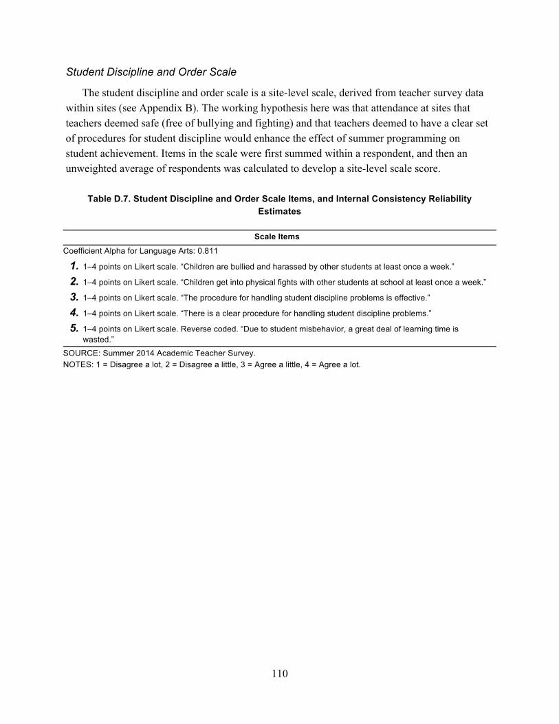
110
Student Discipline and Order Scale
The student discipline and order scale is a site-level scale, derived from teacher survey data within sites (see Appendix B). The working hypothesis here was that attendance at sites that teachers deemed safe (free of bullying and fighting) and that teachers deemed to have a clear set of procedures for student discipline would enhance the effect of summer programming on student achievement. Items in the scale were first summed within a respondent, and then an unweighted average of respondents was calculated to develop a site-level scale score.
Table D.7. Student Discipline and Order Scale Items, and Internal Consistency Reliability Estimates
Scale Items Coefficient Alpha for Language Arts: 0.811
1. 1–4 points on Likert scale. “Children are bullied and harassed by other students at least once a week.” 2. 1–4 points on Likert scale. “Children get into physical fights with other students at school at least once a week.” 3. 1–4 points on Likert scale. “The procedure for handling student discipline problems is effective.” 4. 1–4 points on Likert scale. “There is a clear procedure for handling student discipline problems.” 5. 1–4 points on Likert scale. Reverse coded. “Due to student misbehavior, a great deal of learning time is
wasted.” SOURCE: Summer 2014 Academic Teacher Survey. NOTES: 1 = Disagree a lot, 2 = Disagree a little, 3 = Agree a little, 4 = Agree a lot.

111
Positive School Climate
This scale is also derived from summer classroom observation data and initially calculated at the classroom level. To develop scale scores, we first averaged to the classroom (when classrooms were observed more than once), then the teachers (when teachers were observed more than once), then the site. This site-level estimate is then attributed to each student who attended that site.
Table D.8. Site Climate Scale Items and Internal Consistency Reliability Estimates
Scale Items
Coefficient Alpha: 0.644
1. Average score of 0–1 point, where 1 point assigned if teacher shows explicit signs of positive affect toward youth. Mark no if teacher is simply respectful toward students. Teacher tone is warm and caring. He or she uses positive language, smiles, laughs, or shares good-natured jokes throughout class. If no verbal interaction is necessary, teacher demonstrates a positive and caring affect toward youth.
2. Average score of 0–1 point, where 1 point assigned if students show explicit signs that they have warm, positive affect to teacher (not just respect for teachers). For example, throughout the class they may smile at teacher, laugh with the teacher, or share good-natured jokes.
3. Average score of 0–1 point, where 1 point assigned if students verbally encourage one another, are overtly friendly and supportive.
4. Average score of 0–1 point, where 1 point assigned if students show respect for one another. They refrain from derogatory comments or actions about an individual person and the work he or she is doing; if disagreements occur, they are handled constructively.
5. Average score of 0–1 point, where 1 point assigned if there were no instances where the teacher was disrespectful to students. This includes yelling at one or more students, intimidating or being rude or dismissive to students, using physical aggression, intentionally humiliating or ignoring a student, using discriminatory acts or derogatory language to students.
6. Average score of 0–1 point, where 1 point assigned if there were no instances of flagrant student misbehavior. This includes a physical fight or persistent bullying or persistent use of discriminatory or derogatory language.
7. Average score of 0–1 point, where 1 point assigned if there were no instances where the teacher responsible for the activity was disengaged in the classroom because of distractions by factors that were within her control (i.e., a teacher stopping by to have a conversation about the weekend, the teacher checking his/her cell phone, texting, or taking or making a personal call that was not related to an emergency, personal chat with co-teacher or paraprofessional while students are working).

112
The Daily Climate Scale
This scale draws on a daily survey filled out by a RAND observer at the end of the summer program day. The daily climate scale is the average of the following six RAND observer–rated items (each item is rated at the end of the given observation day), and then averaged over the total number of observation days at the given summer site. The rating for each item was on a five-point scale from 1 (strongly disagree) to 5 (strongly agree). The middle point on the scale represented a neutral response. The items are presented in Table D.9.
Table D.9. Daily Climate Scale items
Scale Items
1. 1–5 points on Likert scale. Adults at the site address student behavior consistently and appropriately when misbehavior occurs
2. 1–5 points on Likert scale. Almost none or no student misbehavior at this site
3. 1–5 points on Likert scale. Site is well-organized (predictable routines, smooth transitions, clear communication among staff)
4. 1–5 points on Likert scale. Students appeared to have enjoyable day
5. 1–5 points on Likert scale. Staff are overtly friendly toward students
6. 1–5 points on Likert scale. Students are overtly friendly toward and supportive of one another
SOURCE: Summer 2014 daily climate observation survey. NOTES: 1 = Strongly disagree, 2 = Disagree, 3 = Neutral, 4 = Agree, and 5 = Strongly agree.
Stand-Alone Moderator Finally, we hypothesized that having a teacher who worked in a proximate grade level during
the prior school year (either third or fourth grade in Year 1, or fourth or fifth grade in Year 2) would moderate the effect of summer programming on students’ mathematics and reading achievement. We reasoned that those teachers would theoretically be versed in the school-year academic standards that applied either in the year preceding or the year following the students’ summer session, and they would be familiar with the most-common gaps between students’ knowledge and these standards. For this item, we simply associated the dichotomous indicator with each treatment group attender via classroom rosters.

113
Appendix E: Statistical Analysis
Analysis Plan
Preferred Random-Effects Model
Our preferred model for ITT analysis of the impact of the summer learning programs is a random-effects model:
𝑌𝑌!"#$% = 𝛼𝛼𝑇𝑇!"#$ + 𝛽𝛽𝑋𝑋!"#$ + 𝛿𝛿𝛿𝛿𝛿𝛿𝛿𝛿𝛿𝛿𝛿𝛿𝛿𝛿𝛿𝛿𝛿𝛿𝛿𝛿𝛿𝛿𝛿𝛿!" + 𝛾𝛾! + 𝜋𝜋! ∗ 𝑍𝑍!"#$ + 𝜇𝜇! ∗ 𝑍𝑍!"#$ + 𝜀𝜀!"#$%
where: • 𝑌𝑌!"#$% is the standardized post-test score in subject q for student i in strata s in summer
site p in summer classroom c, where p and c are defined to be 0 for students who did not attend the summer program.
• 𝑇𝑇!"#$ is a indicator of assignment to the treatment group. • 𝑋𝑋!"#$ is a vector of baseline covariates (see below). • 𝑃𝑃𝑃𝑃𝑃𝑃𝑃𝑃𝑃𝑃𝑃𝑃𝑃𝑃𝑃𝑃𝑃𝑃𝑃𝑃𝑃𝑃!" is a vector of mean pretest values of all students who were assigned to
the same summer classroom in subject q. This is zero for all students who did not attend the summer program. There are four classroom means, one for each of the four pretests (spring 2013 mathematics and LA, and the earlier assessments in mathematics and LA that were used for stratification).
• 𝛾𝛾! are strata fixed-effects (dummy variables). • 𝑍𝑍!"#$ is an indicator variable taking a value of 1 if a student is a member of class c in site
p, used to define random effects. Every student in summer site p and classroom c is associated with a random effect, including those students assigned to treatment who take up the program and those students assigned to control who take up the program (i.e., “crossovers”). This is 0 for the rest of the control-group students and all treatment group students that do not take up treatment (“no-shows”).20
• 𝜋𝜋! ∗ 𝑍𝑍!"#$ is a random-effect common to all students in summer site p. • 𝜇𝜇! ∗ 𝑍𝑍!"#$ is a random-effect common to all students in summer classroom c. • 𝜀𝜀!"#$% is a residual, the variance of which is allowed to vary by pattern of available
pretests. The baseline variables in the model are:
• spring 2013 assessment scores (third grade) in mathematics and LA, standardized within district; interacted with district dummies; missing scores equal to 0
20 This represents a change in the random-effects specification from McCombs et al. (2014). In that report, random-effects were specified based on treatment assignment (rather than class membership). This has the effect of giving random effects to all treatment students, even those that are no-shows, and suppressing random effects for all control students, even those that are cross-overs. These current random effects more accurately reflect the random effects structure with treatment noncompliance. Resulting parameter estimates have shifted slightly from those reported in McCombs et al. (2014), although the general patterns of substantive findings have not changed.

114
• spring 2012 or fall 2012 benchmark assessment scores in mathematics and LA, standardized within district; interacted with district dummies; missing scores equal to 0
• dummy variables for patterns of missing values of the pretests by district • dummy for FRPL • dummy for African American • dummy for Hispanic • dummy for ELL • dummy for special education (exclusive of gifted and talented designation) • dummy for male. • SY 2012–2013 attendance (percentage of school days attended) • dummy for SY 2012–2013 suspension.21
For all results presented throughout this report, we estimated this model using R’s “lme”
command. We made the assumption that the variance of the random effects was constant. We allowed the variance of the residual error to vary across the patterns of missingness in the pretests by district, because the prior scores were likely strong predictors of outcomes, and so the residual variance in outcomes should depend on which and how many prior scores were available.
The R command was:
lme( [outcome var] ~ [treatment var] + [baseline variables in X] + [pre-test classroom means] + [strata dummies] + [missing data pattern indicators], random = list(dumid = [summer site and classroom dummies]),22 weights = varIdent(form = ~1 | [missing data pattern indicators]))23
Secondary analyses used simple extensions to this model. In the case of attendance and academic time-on-task models, the treatment assignment indicator was replaced with continuous or categorical variables for these mediators. These models are detailed below. When testing other mediators or moderators (such as student characteristics, or class/site characteristics), the variable of interest was interacted with the treatment indicator.
21 These covariates became available and were added after the publication of McCombs et al. (2014). 22 The random effect specification in the R command is adapted from Lockwood, Doran, and McCaffrey (2003), which describes a flexible approach to specifying groupings, including the partial nesting of only treatment students in summer sites and classes, and the additional complexity of cross-classification that will results from students having different site and class assignments in the two summers of this experiment. With complete compliance, this specification is equivalent to the specifications outlined in Lohr, Schochet and Sanders (2014) used to analyze partially nested experimental designs. 23 For the fall 2013 analyses, models were also estimated using STATA’s “xtmixed” command using the code:
xtmixed [outcome var] [treatment var] [baseline variables in X] [strata dummies] [pre-test classroom means] || [summer site and classroom ID variables]: [summer site and classroom dummies] , nocons covariance(identity) , reml

115
Attendance and Academic Time-on-Task Analysis
Our preferred model for attendance and academic time on task analysis is a modification of the random-effects model used for the ITT analysis:
𝑌𝑌!"#$% = 𝛼𝛼𝑊𝑊!"#$ ∗ 𝑇𝑇!"#$ + 𝛽𝛽𝑋𝑋!"#$ + 𝛿𝛿𝛿𝛿𝛿𝛿𝛿𝛿𝛿𝛿𝛿𝛿𝛿𝛿𝛿𝛿𝛿𝛿𝛿𝛿𝛿𝛿𝛿𝛿!" + 𝛾𝛾! + 𝜋𝜋! ∗ 𝑍𝑍!"#$ + 𝜇𝜇! ∗ 𝑍𝑍!"#$ + 𝜀𝜀!"#$%
where variables are defined as above, and • 𝑊𝑊!"#$ is a categorical variable indicating academic time on task or attendance category
membership (“no show,” “low” or “high”)
Robustness Checks
In addition to our preferred model, we estimated three additional models to test the robustness of our ITT estimates on the fall 2013 outcomes.
1. random effects, no baseline covariates 2. ordinary least squares (OLS) regression models with bootstrap-based inference, baseline
covariates 3. OLS with bootstrap-based inference, no baseline covariates.
Model 1 acted as a check that the inclusion of baseline controls was not driving the estimate of the ITT. We expected the model with baseline covariates would have a similar point estimate but a much smaller standard error because of the variance reduction from controlling for the pretests. We found that the resulting point estimates were similar to the preferred model because covariates were well balanced across the experimental groups because of randomization. The statistical significance of the estimates in this model were not used to judge whether the summer programs had an effect.
Models 2 and 3 were estimated to address the potential concern that our preferred model requires parametric assumptions about the form of the clustering induced by the program being delivered in summer classrooms (and assumes there is no clustering between any students in the control group). Model 2 contains the same covariates as the random-effects model, but uses ordinary least squares estimation. We conducted statistical inferences making fewer parametric assumptions and also allowed a more general form of clustering. Model 3 contains no covariates and is a bit more conservative than Model 2, in that it can produce slightly larger standard errors.
In order to estimate Models 2 and 3, we defined clusters corresponding to each summer site. We then considered each sending school to be a member of exactly one of these summer site clusters, defined as the summer site to which the majority of the school’s treatment group students were sent for summer 2013. Once the clusters were determined in this manner, all treatment students were assigned to the cluster where they actually attended during summer 2013. All control group students (as well as nonattending treatment group students) were assigned to clusters on the basis of their sending school at the time of randomization in spring

116
2013. This resulted in all students in a summer site or classroom being defined to be in the same cluster, regardless of their actual regular-year schools, thus accounting for any clustering generated at the summer site and classroom levels.
The number of resulting clusters was less than 40 (because the number of summer sites was fewer than 40), so we were concerned about using the usual Huber-Eicker-White sandwich estimator cluster adjustment, which requires a large number of clusters to be valid. Instead, we used the bootstrap procedure discussed by Cameron, Gelbach, and Miller (2008) to calculate p values for the null hypothesis that the treatment had zero effect. Our analyses confirmed that results from the OLS and random-effects models were substantively the same.24
Analysis of Treatment Effect on the Treated To estimate the effect of attendance in the summer program (i.e., the TOT),25 we had to
account for the fact that selection into program attendance in the treatment group was endogenous. Therefore, we used randomization status as an instrumental variable for program attendance. Specifically, we estimated via two-stage least squares models of the form:
Yic = θTic + dc + X’
icβ + εic Tic = αZic + dc + X’
icφ + εic
where Tic is a binary indicator of whether the student attended any days of the summer program.26 Now, the parameter of interest is θ, the coefficient on Tic in the outcome equation. This parameter captured the average effect of the intervention for the subgroup of students who participated in the program (Angrist, Imbens, and Rubin, 1996; Bloom, 2006). P values were derived using the wild cluster bootstrap-t procedure proposed by Cameron, Gelbach, and Miller (2008) for situations where the number of clusters is small. In this application, clusters were determined by summer site. For students in the control group, we used the summer site that most treated students in a student’s regular-year school attended.
Multiple Hypotheses Testing
When performing multiple hypothesis tests on a data set, the chance of erroneously finding statistically significant results (i.e., Type I errors) increases as the number of tests increase. As a consequence, we adopted a standard corrective measure, which was to apply more-stringent
24 As an additional robustness check, we calculated ITT using the approaches outlined in Jo, Asparouhov, and Muthen (2008). The results of these analyses were also substantively the same as our preferred model. 25 Technically, given the fact that there are both “no-shows” and “crossovers”, these TOT estimates actually represent complier average causal effects or local average treatment effects. See Bloom and Weiland (2014) for details. 26 For fall 2014 and spring 2015 analyses, Tic is a binary indicator of whether the student attended any days of the summer program in either year.

117
criteria for determining statistical significance. In practice, this translated into lowering the critical p value for determining statistical significance to something less than 0.05. Exactly how much lower than 0.05 was determined by the number of tested hypotheses that pertain to a given domain of outcomes and the specific correction method used.
The exact methods and decisions to make when employing these corrections are a matter of debate among statisticians. After reviewing the spectrum of most conservative to most liberal options, we adopted a middle-ground position that adheres to the most detailed guidance that IES has released on this topic (Schochet, 2008).
Consistent with WWC standards, we used the Benjamini-Hochberg method of controlling the false discovery rate (Benjamini and Hochberg, 1995). Following Schochet’s (2008) guidance, we defined seven student outcome domains pertinent to the summer learning demonstration:
1. mathematics outcomes 2. reading outcomes 3. end of course mathematics grades 4. end of course LA grades 5. social-emotional outcomes 6. school-year behavior (e.g., suspensions ) 7. school-year attendance.
Only those hypotheses that belonged to a confirmatory category of an outcome domain were subject to corrections for multiple hypotheses testing within that domain. Exploratory hypotheses were not subject to multiple hypotheses corrections. For domain-specific confirmatory analyses in each district summer learning demonstration report, we adjusted downward the critical p value for determining statistical significance according to the number of total hypotheses tests belonging to that domain for the period from 2013 to 2017. Table E.1 enumerates the confirmatory hypotheses tests conducted in each domain at each time point.
Table E.1. Number of Hypothesis Test for Each Outcome Domain for Each Study Time Point
Domain
Year
Total 2013 2014 2015 2016 2017
Mathematics assessments 15 30 9 0 9 63 Reading assessments 15 30 9 0 9 63 End-of-course mathematics grades 0 7 7 0 7 21 End-of-course LA grades 0 7 7 0 7 21 Social-emotional outcomes 15 15 0 0 9 39 School-year behavior 0 7 7 0 7 21 School-year attendance 0 7 7 0 7 21

118
Meta-Analysis While the reading, mathematics, and social-emotional outcomes are collected using the same
instruments in all districts in fall 2013 and in fall 2014, the spring outcomes are not uniformly captured across districts. For example, different states administer different standardized assessments, and districts use different scales for course grades, and track suspensions differently. In order to obtain ITT and TOT estimates for outcomes that use disparate measures across districts, we use a meta-analytic approach. Meta-analysis pools results from individual studies to obtain a summary estimate of effects (Glass, 1976; Nordmann, Kasenda, and Briel, 2012). In this case, we treat each district as a separate study, and then obtain an overall ITT or TOT estimate by synthesizing district-specific estimates. Because meta-analysis uses effect sizes to describe outcome variables, the outcomes are on a common metric, and are not sensitive to differences in assessments or other outcomes across sites (e.g., Yin, Schmidt, and Besag, 2006).
The current study applies a fixed-effect model to meta-analyze the data across the five study districts. First, a treatment effect is estimated in each district, along with a standard error for that effect. Then, the following model is employed:
𝑇𝑇! = 𝜇𝜇 + 𝜀𝜀! where 𝑇𝑇! is the observed treatment effect (ITT or TOT estimate) in district i, 𝜇𝜇 is the overall effect, and 𝜀𝜀! is within-district error. An estimate of the overall treatment effect (across k districts) is given by:
𝑇𝑇∙ =
1𝑣𝑣!𝑇𝑇!!
! ! !
1𝑣𝑣!
!! ! !
where 𝑣𝑣! describes the within-district variance. Greater within-district variance means that there is more measurement error and, as such, effect estimates are less precise. 𝑇𝑇∙ is essentially a precision-weighted average of a treatment effect across the k districts. Districts with less measurement error are given more weight in the calculation of this average than districts with more measurement error (Borenstein, Rothstein, and Hedges, 2007).
We also employed techniques from meta-analysis (Hedges, 1982; Rosenthal and Rubin, 1982) to formally investigate heterogeneity in the magnitude of district specific effects.
We estimate these models in R using the “rmeta” software package (Lumley, 2012).
Linear Probability Models
Student suspension data analysis involved a binary outcome (i.e., 1 if suspended once or more during SY 2013–2014, 0 otherwise). We opted to analyze suspension data using a linear probability model (LPM), which substitutes a binary outcome into the existing random effects modeling framework outlined above.
Some researchers recommend using nonlinear response models (e.g., generalized linear models with logistic or probit link functions) with binary outcomes, and note that LPMs can

119
result in predicted probabilities that are out of range or have inappropriate standard errors (Mood, 2010). However, under general conditions (and when the true data-generating mechanism is unknown),27 the linear probability model may be a better choice than a logit model, particularly if the coefficients of the linear probability model are interpreted as average marginal effects on probabilities (Mood, 2010; Pischke, 2012). Additionally, omitted variables in logistic regression can influence parameter estimation even when variables are not correlated with variables already included in the model (Mood, 2010), and adding covariates into a logit model can actually decrease precision and increase standard errors (Robinson and Jewell, 1991).28
27 The data-generating mechanism describes the underlying process by which observed data are believed to have originated. An important aspect of statistical inference is selecting a model that is compatible with the generating mechanism, what is sometimes called the selection problem (Spanos, 2006). With real-world observed data (as opposed to simulated data) that true process is often unknown. 28 A secondary advantage of LPM in this situation is that the models for binary outcomes will have the same specification as our preferred model for continuous outcomes—that is, a complex hierarchical model with clustering only in the experimental arm and which allows variance of the residual error to vary across the patterns of missing data in pretest covariates. It likely would have been difficult or impossible to retain these features in a logistic regression framework.

120
Appendix F: Results from Regression Models
In this appendix, we report in tabular format the results narratively described in Chapters Four and Five of the main report. As described in Appendix E, all models included a rich set of covariates; however, here, we only report the regression coefficients of interest.
Table F.1. ITT Results, Overall
Analyses Fall 2013
Estimate (SE) Spring 2014
Estimate (SE) Fall 2014
Estimate (SE) Spring 2015
Estimate (SE)
Mathematics Analyses Achievement 0.08* (0.02) 0.04 (0.02) 0.03 (0.02) 0.04 (0.02) End-of-year grades 0.01 (0.02) 0.00 (0.02)
Reading Analyses Achievement 0.00 (0.02) 0.01 (0.02) 0.04 (0.02) 0.03 (0.02) End-of-year grades 0.01 (0.01) 0.00 (0.02)
Social-Emotional and Behavioral Analyses Social-emotional assessment 0.02 (0.02) 0.05 (0.03) Suspensions 0.00 (0.01) –0.01 (0.01) Attendance 0.00 (0.00) 0.00 (0.00)
* Indicates statistical significance at the p < 0.05 level after applying the Benjamini-Hochberg correction for multiple hypothesis tests.
Table F.2. Counts of Students Participating in ITT Analyses
Analysis Fall 2013 Spring 2014 Fall 2014 Spring 2015
Control Treat Control Treat Control Treat Control Treat
Mathematics Analyses Achievement 2,205 2,921 2,218 2,920 1,952 2,553 1,870 2,431 End-of-year grades 2,173 2,889 1,931 2,527
Reading Analyses Achievement 2,196 2,902 2,215 2,915 1,940 2,544 1,885 2,452 End-of-year grades 2,179 2,886 1,930 2,534
Social-Emotional and Behavioral Analyses Social-emotional assessment 1,903 2,542 1,579 2,144
Suspensions 2,308 3,023 2,067 2,715 Attendance 2,306 3,023 2,067 2,715

121
Table F.3. Counts of Students Participating in Subgroup Analyses (Fall Analyses)
Mathematics Reading Social-Emotional
Subgroups
N Control
N Treat
N Control
N Treat
N Control
N Treat
Fall 2013 ELL No 1,447 2,057 1,435 2,045 1,268 1,810
Yes 758 864 761 857 635 732 FRPL-eligible (excl. Boston) No 182 258 179 255 162 233
Yes 1,677 2,139 1,670 2,120 1,466 1,898 Below median on prior achievement
No 1,100 1,460 1,092 1,459 946 1,256 Yes 1,105 1,461 1,104 1,443 957 1,286
Fall 2014 ELL No 1,255 1,768 1,251 1,772 1,044 1,507
Yes 697 785 689 772 535 637 FRPL-eligible (excl. Boston) No 182 258 179 255 162 233
Yes 1,677 2,139 1,670 2,120 1,466 1,898 Level 1 in either subject No 1,134 1,495 1,129 1,499 917 1,245
Yes 818 1,058 811 1,045 662 899 Spring 2014
ELL No 1,455 2,064 1,455 2,062 Yes 763 856 760 853
FRPL-eligible (excl. Boston) No 185 257 184 256 Yes 1,691 2,137 1,691 2,135
Level 1 in either subject No 1,301 1,723 1,297 1,718 Yes 917 1,197 918 1,197
Spring 2015 ELL No 1,183 1,666 1,198 1,688
Yes 687 765 687 764 Level 1 in either subject No 1,104 1,473 1,110 1,480
Yes 766 958 775 972 NOTE: To calculate students’ prior achievement, we used the control group’s performance on the common GRADE/GMADE posttests to scale each district’s pretests. The posttests were scaled to have a mean of zero, a standard deviation of one, then we calculated the mean and standard deviation of the pretests for the control group subsample in each district, excluding crossovers. Then, each district’s pretests for the whole sample were scaled to have the district’s calculated means and standard deviations.

122
Table F.4. Results of Subgroup Analyses
Subgroup Fall 2013
Estimate (SE) Spring 2014
Estimate (SE) Fall 2014
Estimate (SE) Spring 2015
Estimate (SE)
Mathematics Achievement ELL 0.00 (0.04) –0.05 (0.05) 0.01 (0.04) 0.02 (0.05) FRPL-eligible (excl. Boston) 0.04 (0.06) 0.03 (0.06) –0.02 (0.07) Below median on prior achievement
–0.05 (0.03)
Level 1 in mathematics 0.02 (0.04) –0.02 (0.04) 0.00 (0.05) Reading Achievement
ELL –0.01 (0.04) –0.06 (0.05) –0.01 (0.04) 0.09 (0.06) FRPL-eligible (excl. Boston) 0.05 (0.05) 0.07 (0.07) –0.02 (0.07) Below median on prior achievement
0.02 (0.03)
Level 1 in reading –0.01 (0.05) 0.02 (0.04) –0.03 (0.04) Social-Emotional Assessment
ELL 0.02 (0.05) –0.04 (0.06) FRPL-eligible (excl. Boston) 0.05 (0.09) 0.11 (0.11) Below median on prior achievement
0.11 (0.05)
Level 1 in either subject –0.07 (0.06)
Table F.5. Results of Subscale Analyses
Subgroup Fall 2013
Estimate (SE) Fall 2014
Estimate (SE)
Mathematics Math operations subscale 0.10* (0.02) 0.03 (0.02) Math concepts subscale 0.08* (0.02) 0.04 (0.02) Math process subscale 0.04 (0.02) 0.01 (0.02)
Reading Reading comprehension subscale 0.01 (0.02) 0.03 (0.02) Reading vocabulary subscale 0.01 (0.02) 0.06 (0.02) Reading listening subscale –0.04 (0.03) 0.02 (0.04)
Social-Emotional Self-regulation 0.01 (0.03) 0.04 (0.03) Self-motivation 0.03 (0.02) 0.07 (0.03)
* Indicates statistical significance at the p < 0.05 level after applying the Benjamini-Hochberg correction for multiple hypothesis tests.

123
Table F.6. Results of Treatment-on-the-Treated Analyses
Analyses Fall 2013
Estimate (SE) Spring 2014
Estimate (SE) Fall 2014
Estimate (SE) Spring 2015
Estimate (SE) Mathematics Analyses
Achievement 0.11* (0.03) 0.06 (0.02) 0.04 (0.03) 0.04 (0.02)
End-of-Year Grades 0.01 (0.01) –0.01 (0.02)
Reading Analyses Achievement 0.02 (0.02) 0.01 (0.02) 0.05 (0.02) 0.03 (0.02) End-of-Year Grades 0.01 (0.01) 0.00 (0.01)
Social-Emotional and Behavioral Analyses Social-Emotional Assessment 0.02 (0.02) 0.07 (0.04) Suspensions –0.79% (0.01) –1.21% (0.01) Attendance 0.00% (0.00) 0.00% (0.00)
* Indicates statistical significance at the p < 0.05 level after applying the Benjamini-Hochberg correction for multiple hypothesis tests.
Table F.7. Nonexperimental Linear Effect of Attendance and Academic Time on Task
Characteristic Fall 2013
Estimate (SE) Fall 2014
Estimate (SE)
Mathematics Attendance 0.04* (0.02) 0.03 (0.02) Academic time on task (instructional hours) 0.04* (0.01) 0.04 (0.02)
Reading Attendance 0.02 (0.02) 0.02 (0.02) Academic time on task (instructional hours) 0.02 (0.01) 0.03 (0.02)
Social-Emotional Attendance 0.02 (0.03) 0.04 (0.03)
* Indicates statistical significance at the p < 0.05 level.
Table F.8a. Nonexperimental Effect of Attendance Categories
Characteristic Fall 2013
Estimate (SE) Spring 2014
Estimate (SE) Fall 2014
Estimate (SE) Spring 2015
Estimate (SE)
Mathematics Achievement No-show 0.00 (0.03) 0.00 (0.03) –0.01 (0.02) 0.01 (0.03) Low 0.07* (0.02) 0.02 (0.03) 0.02 (0.03) –0.01 (0.04) High 0.13* (0.02) 0.07* (0.02) 0.11* (0.03) 0.14* (0.03) Attended summer 2013 only –0.01 (0.03) 0.00 (0.03) Attended summer 2014 0.08* (0.02) 0.08* (0.03) Attended summer 2014 only –0.03 (0.05) 0.05 (0.05) Attended both summers 0.09* (0.03) 0.08* (0.03) High attendance both summers 0.10* (0.03) 0.12* (0.03) Students who attended Year 1 only 0.08* (0.03) –0.01 (0.03)
* Indicates statistical significance at the p < 0.05 level.

124
Table F.8a—Continued
Characteristic Fall 2013
Estimate (SE) Spring 2014
Estimate (SE) Fall 2014
Estimate (SE) Spring 2015
Estimate (SE) Reading Achievement No-show –0.03 (0.03) 0.02 (0.03) 0.01 (0.02) 0.01 (0.03) Low –0.01 (0.02) –0.05 (0.03) 0.05 (0.03) 0.03 (0.04) High 0.02 (0.02) 0.03 (0.02) 0.08* (0.03) 0.09* (0.03) Attended summer 2013 only –0.01 (0.03) –0.01 (0.03) Attended summer 2014 0.07* (0.02) 0.07* (0.03) Attended summer 2014 only 0.01 (0.05) 0.07 (0.06) Attended both summers 0.08* (0.02) 0.07* (0.03) High attendance both summers 0.10* (0.03) 0.10* (0.03) Students who attended Year 1 only 0.01 (0.02) –0.02 (0.03) Social-Emotional Assessment No-show 0.05 (0.04) 0.04 (0.04) Low –0.02 (0.04) –0.02 (0.05) High 0.02 (0.03) 0.12* (0.04) Attended summer 2013 only 0.02 (0.04) Attended summer 2014 0.07 (0.04) Attended summer 2014 only 0.13 (0.08) Attended both summers 0.06 (0.04) High attendance both summers 0.14* (0.04) Students who attended Year 1 only 0.03 (0.04) 0.04 (0.05) Mathematics Grades No-show –0.01 (0.02) 0.00 (0.02) Low 0.02 (0.02) –0.03 (0.03) High 0.02 (0.02) 0.03 (0.03) Attended summer 2013 only –0.02 (0.03) Attended summer 2014 0.01 (0.02) Attended summer 2014 only –0.03 (0.05) Attended both summers 0.01 (0.03) High attendance both summers 0.04 (0.03) LA Grades No-show 0.00 (0.02) 0.01 (0.02) Low 0.01 (0.02) 0.00 (0.03) High 0.01 (0.02) –0.01 (0.02) Attended summer 2013 only –0.01 (0.02) Attended summer 2014 –0.01 (0.02) Attended summer 2014 only 0.01 (0.04) Attended both summers –0.01 (0.02) High attendance both summers 0.01 (0.03) Suspensions No-show 0.1% (0.01) –1.2% (0.01) Low –0.3% (0.01) –0.1% (0.01) High –0.1% (0.01) –1.5% (0.01) Attended summer 2013 only –1.0% (0.01) Attended summer 2014 –1.3% (0.01) Attended summer 2014 only –0.7% (0.02) Attended both summers –1.3% (0.01) High attendance both summers –2.1% (0.01) * Indicates statistical significance at the p < 0.05 level.

125
Table F.8b. Nonexperimental Effect of Academic Time on Task Categories
Characteristic Fall 2013
Estimate (SE) Spring 2014
Estimate (SE) Fall 2014
Estimate (SE) Spring 2015
Estimate (SE)
Mathematics Achievement No-show 0.00 (0.03) 0.00 (0.03) –0.01 (0.02) 0.01 (0.03) Low (< 25.5 instructional hours) 0.08* (0.02) 0.04 (0.02) 0.03 (0.03) 0.06 (0.03) High (> = 25.5 instructional hours) 0.16* (0.03) 0.05 (0.03) 0.13* (0.03) 0.11* (0.03) High academic time on task both summers 0.13* (0.04) 0.09* (0.04)
Reading Achievement No-show –0.03 (0.03) 0.02 (0.03) 0.01 (0.02) 0.01 (0.03) Low (< 34 instructional hours) –0.01 (0.02) –0.01 (0.02) 0.06* (0.03) 0.05 (0.03) High (> = 34 instructional hours) 0.05* (0.02) 0.03 (0.03) 0.09* (0.03) 0.13* (0.04) High academic time on task both summers 0.07 (0.04) 0.12* (0.05)
Mathematics Grades No-show –0.01 (0.02) 0.00 (0.02) Low (< 25.5 instructional hours) 0.02 (0.02) –0.01 (0.03) High (> = 25.5 instructional hours) 0.02 (0.02) 0.03 (0.03)
ELA Grades No-show 0.00 (0.02) 0.01 (0.02) Low (< 34 instructional hours) 0.01 (0.02) –0.01 (0.03) High (> = 34 instructional hours) 0.02 (0.02) –0.01 (0.03)
* Indicates statistical significance at the p < 0.05 level.
Table F.9. Nonexperimental Effects of Camp Attendance According to Student Survey
Characteristic Fall 2013
Estimate (SE) Fall 2014
Estimate (SE)
Mathematics Attended camp w/mathematics > = a few weeks, control 0.02 (0.03) –0.12* (0.05) Did not attend camp w/mathematics ≥ a few weeks, treatment 0.00 (0.02) 0.03 (0.02) Attended camp w/mathematics ≥ a few weeks, treatment 0.14* (0.02) –0.12 (0.07)
Reading Attended camp w/reading ≥ a few weeks, control 0.01 (0.03) 0.04 (0.06) Did not attend camp w/reading ≥ a few weeks, treatment –0.04* (0.02) 0.04 (0.02) Attended camp w/reading ≥ a few weeks, treatment 0.04* (0.02) 0.02 (0.07)
Social-Emotional Attended camp ≥ a few weeks, control –0.06 (0.04) 0.06 (0.05) Did not attend camp ≥ a few weeks, treatment 0.01 (0.04) 0.09 (0.05) Attended camp ≥ a few weeks, treatment –0.01 (0.03) 0.12* (0.06)
* Indicates statistical significance at the p < 0.05 level.

126
Table F.10. Nonexperimental Estimates of the Effect of Relative Opportunity for Instruction
Characteristic Fall 2013
Estimate (SE) Fall 2014
Estimate (SE)
Mathematics Relative opportunity for instruction 0.01 (0.02) 0.04 (0.03)
Reading Relative opportunity for instruction 0.00 (0.02) 0.01 (0.02)
Table F.11. Nonexperimental Estimates of Moderation
Characteristic Fall 2013
Estimate (SE) Spring 2014
Estimate (SE) Fall 2014
Estimate (SE) Spring 2015
Estimate (SE)
Mathematics Mathematics classroom instructional quality scale 0.00 (0.01) 0.01 (0.01) 0.02 (0.02) –0.02 (0.02)
Positive school climate 0.01 (0.02) 0.02 (0.02) Daily climate scale 0.01 (0.02) Good fit mathematics curriculum 0.00 (0.02) 0.03 (0.04) Student discipline and order 0.00 (0.02) –0.03 (0.03) –0.02 (0.02) 0.04 (0.03) Mathematics teacher taught subject in adjacent grade prior school year 0.03 (0.03) 0.03 (0.03) –0.03 (0.04) –0.04 (0.05)
Reading LA classroom instructional quality scale 0.05* (0.01) 0.01 (0.02) 0.01 (0.02) 0.02 (0.02)
Positive school climate –0.01 (0.01) 0.00 (0.02) Daily climate scale 0.00 (0.02) Good fit LA curriculum 0.00 (0.01) –0.01 (0.04) Student discipline and order 0.04* (0.02) 0.04 (0.03) 0.00 (0.02) –0.02 (0.03) LA teacher taught subject in adjacent grade prior school year 0.09* (0.03) 0.04 (0.03) 0.00 (0.04) –0.02 (0.05)
Social-Emotional Positive school climate 0.00 (0.02) 0.01 (0.03) Daily climate scale –0.04 (0.03) Student discipline and order 0.04 (0.02) 0.04 (0.03)
Mathematics Grades Mathematics classroom instructional quality scale 0.01 (0.01) –0.03 (0.02)
Student discipline and order 0.00 (0.02) 0.01 (0.03) Mathematics teacher taught subject in adjacent grade prior school year –0.02 (0.03) –0.05 (0.05)

127
Table F.11—Continued
Characteristic Fall 2013
Estimate (SE) Spring 2014
Estimate (SE) Fall 2014
Estimate (SE) Spring 2015
Estimate (SE)
LA Grades LA classroom instructional quality scale 0.02 (0.01) 0.00 (0.02) Student discipline and order –0.01 (0.02) 0.01 (0.02) LA teacher taught subject in adjacent grade prior school year 0.04 (0.03) 0.02 (0.04)
Suspensions Positive school climate –1.6% (0.01) –0.7% (0.01) Student discipline and order 0.7% (0.01) –0.9% (0.01)
Attendance High instructional quality in LA or mathematics –0.1% (0.00) –0.1% (0.00)
Positive school climate 0.00% (0.00) –0.2%(0.00) Student discipline and order 0.1% (0.00) –0.3% (0.00)
128
References
Alexander, Karl L., Doris R. Entwisle, and Linda Steffel Olson, “Lasting Consequences of the Summer Learning Gap,” American Sociological Review, Vol. 72, No. 2, 2007, pp. 167–180.
Allington, Richard L., Anne McGill-Franzen, Gregory Camilli, Lunetta Williams, Jennifer Graff, Jacqueline Zeig, Courtney Zmach, and Rhonda Nowak, “Addressing Summer Reading Setback Among Economically Disadvantaged Elementary Students,” Reading Psychology, Vol. 31, No. 5, October 2010, pp. 411–427.
Angrist, Joshua D., Guido W. Imbens, and Donald B. Rubin, “Identification of Causal Effects Using Instrumental Variables,” Journal of the American Statistical Association, Vol. 91, No. 434, 1996, pp. 444–455.
Arbreton, Amy J. A., Jean Baldwin Grossman, Carla Herrera, and Leigh L. Linden, Testing the Impact of Higher Achievement’s Year-Round Out-of-School-Time Program on Academic Outcomes, New York: Public/Private Ventures, 2011. As of March 21, 2016: http://ppv.issuelab.org/resource/testing_the_impact_of_higher_achievements_year_round_out_of_school_time_program_on_academic_outcomes
Atteberry, Allison, Andrew McEachin, and Aryn Bloodworth, “School’s Out: Summer Learning Loss Across Grade Levels and School Contexts in the U.S. Today,” in K. Alexander, M. Boulay, and S. Pitcock, eds., Summer Learning and Summer Learning Loss: Theory, Research and Practice, New York: Teachers College Press, forthcoming.
Augustine, Catherine H., Jennifer Sloan McCombs, Heather L. Schwartz, and Laura Zakaras, Getting to Work on Summer Learning: Recommended Practices for Success, Santa Monica, Calif.: RAND Corporation, RR-366-WF, 2013. As of March 18, 2016: http://www.rand.org/pubs/research_reports/RR366.html
Benjamini, Yoav, and Yosef Hochberg, “Controlling the False Discovery Rate: A Practical and Powerful Approach to Multiple Testing,” Journal of the Royal Statistical Society, Series B (Methodological), Vol. 57, No. 1, 1995, pp. 289–300.
Benson, James, and Geoffrey Borman, “Family, Neighborhood, and School Settings Across Seasons: When Do Socioeconomic Context and Racial Composition Matter for the Reading Achievement Growth of Young Children? Teachers College Record, Vol. 112, No. 5, 2010, pp. 1338–1390.

129
Bloom, Howard S., The Core Analytics of Randomized Experiments for Social Research MDRC Working Papers on Research Methodology, MDRC Working Papers on Research Methodology, New York: MDRC, 2006. As of October 22, 2014: http://www.mdrc.org/sites/default/files/full_533.pdf
Bloom, Howard, and Christina Weiland, Quantifying Variation in Head Start Effects on Young Children’s Cognitive and Socio-Emotional Skills Using Data from the National Head Start Impact Study, New York: MRDC, 2014. As of April 13, 2016: http://www.mdrc.org/sites/default/files/quantifying_variation_in_head_start.pdf
Borenstein, Michael, Larry Hedges, and Hannah Rothstein, Meta-Analysis: Fixed Effect vs. Random Effects, Meta-Analysis.com, 2007.
Borman, Geoffrey D., James Benson, and Laura T. Overman, “Families, Schools, and Summer Learning,” Elementary School Journal, Vol. 106, 2005, pp. 131–150.
Borman, Geoffrey D., and N. Maritza Dowling, “Longitudinal Achievement Effects of Multiyear Summer School: Evidence from the Teach Baltimore Randomized Field Trial,” Educational Evaluation and Policy Analysis, Vol. 28, No. 1, 2006, pp. 25–48.
Borman, Geoffrey D., Michael Goetz, and N. Maritza Dowling, “Halting the Summer Achievement Slide: A Randomized Field Trial of the KindergARTen Summer Camp,” Journal of Education for Students Placed at Risk (JESPAR), Vol. 14, No. 2, April 2009, pp. 133–147.
Burkham, David T., Douglas D. Ready, Valerie E. Lee, and Laura F. LoGerfo, “Social-Class Differences in Summer Learning Between Kindergarten and First Grade: Model Specification and Estimation,” Sociology of Education, Vol. 77, No. 1, 2004, pp. 1–31.
Cameron, A. Colin, Jonah B. Gelbach, and Douglas L. Miller, “Bootstrap-Based Improvements for Inference with Clustered Errors,” Review of Economics and Statistics, Vol. 90, No. 3, 2008, pp. 414–427.
Chaplin, Duncan, and Jeffrey Capizzano, Impacts of a Summer Learning Program: A Random Assignment Study of Building Educated Leaders for Life (BELL), Washington, D.C.: Urban Institute, 2006.
Coleman, J. S., E. Q. Campbell, C. J. Hobson, J. McPartland, A. M. Mood, F. D. Weinfeld, et al., Equality of Educational Opportunity. Washington, D.C.: U.S. Government Printing Office, 1966.
Cooper, Harris, Kelly Charlton, Jeff C. Valentine, Laura Muhlenbruck, and Geoffrey D. Borman, Making the Most of Summer School: A Meta-Analytic and Narrative Review, Vol. 65, Monographs of the Society for Research in Child Development, Malden, Mass.: Blackwell Publishers, 2000.

130
Cooper, Harris, Barbara Nye, Kelly Charlton, James Lindsay, and Scott Greathouse, “The Effects of Summer Vacation on Achievement Test Scores: A Narrative and Meta-Analytic Review,” Review of Educational Research, Vol. 66, No. 3, 1996, pp. 227–268.
Danielson Group, “Promoting Effective Teaching and Professional Learning,” website, 2013. As of March 23, 2016: http://www.danielsongroup.org/
Downey, Douglas B., Paul T. Von Hippel, and Beckett A. Broh, “Are Schools the Great Equalizer? Cognitive Inequality During the Summer Months and the School Year,” American Sociological Review, Vol. 69, No. 5, 2004, pp. 613–635.
Duflo, Esther, Rachel Glennerster, and Michael Kremer, “Using Randomization in Development Economics: A Toolkit,” in T. P. Schults and J. A. Strauss, eds., Handbook of Development Economics, Vol. 4, Amsterdam: North-Holland, Elsevier B.V., 2007, pp. 3862–3895.
Eicker, Friedhelm, “Limit Theorems for Regression with Unequal and Dependent Errors,” Proceedings of the Fifth Berkeley Symposium on Mathematical Statistics and Probability, Vol. 1, Berkeley, Calif.: University of California Press, 1967, pp. 59–82.
Entwisle, Doris R., and Karl L. Alexander, “Beginning School Math Competence: Minority and Majority Comparisons,” Child Development, Vol. 61, No. 2, 1990, pp. 454–471.
———, “Summer Setback: Race, Poverty, School Composition, and Mathematics Achievement in the First Two Years of School,” American Sociological Review, Vol. 57, No. 1, 1992, pp. 72–84.
Entwisle, Doris R., Karl L. Alexander, and Linda Steffel Olson, “Keep the Faucet Flowing: Summer Learning and Home Environment,” American Educator, Vol. 25, No. 3, Fall 2001, pp. 10–15, 47.
Fisher, Charles W., David C. Berliner, Nikola N. Filby, Richard Marliave, Leonard S. Cahen, and Marilyn M. Dishaw, “Teaching Behaviors, Academic Learning Time, and Student Achievement: An Overview,” in Carolyn Denham and Ann Lieberman, eds., Time to Learn: A Review of the Beginning Teacher Evaluation Study, Sacramento, Calif.: California State Commission for Teacher Preparation and Licensing, 1980, pp. 7–32.
Gershenson, Seth, “Do Summer Time-Use Gaps Vary by Socioeconomic Status?” American Educational Research Journal, Vol. 50, No. 6, 2013, pp. 1219–1248.
Gershenson, Seth, Alison Jacknowitz, and Andrew Brannegan, “Are Student Absences Worth the Worry in U.S. Primary Schools?” Bonn, Germany: Institute for the Study of Labor (IZA), IZA DP No. 9558, 2015. As of March 21, 2016: http://ftp.iza.org/dp9558.pdf

131
Glass, Gene V., “Primary, Secondary, and Meta-Analysis of Research,” Educational Researcher, Vol. 5, No. 10, 1976, pp. 3–8.
Gottfried, Michael, “Excused Versus Unexcused: How Student Absences in Elementary School in Elementary School Affect Academic Achievement,” Educational Evaluation and Policy Analysis, Vol. 31, No. 4, 2009, pp. 392–419.
———, “The Detrimental Effects of Missing School: Evidence from Urban Siblings,” American Journal of Education, Vol. 117, No. 2, 2011, pp. 147–182.
Guryan, Johnathan, James S. Kim, and Kyung Park, Motivation and Incentives in Education: Evidence from a Summer Reading Experiment, Cambridge, Mass.: National Bureau of Economic Research, NBER Working Paper 20918, 2015. As of March 21, 2016: http://www.nber.org/papers/w20918
Harnischfeger, Annegret, and David E. Wiley, “The Teaching-Learning Process in Elementary Schools: A Synoptic View,” Curriculum Inquiry, Vol. 6, No. 1, 1976, pp. 5–43.
Hawley, Willis D., Susan Rosenholtz, Henry J. Goodstein, and Ted Hasselbring, “Good Schools: What Research Says About Improving Student Achievement,” Peabody Journal of Education, Vol. 61, No. 4, 1984, pp. iii–178.
Hayes, Michael S., and Seth Gershenson, “The Estimation of Summer Learning Rates,” paper presented at the 2014 AEFP Annual Conference, San Antonio, Tex., 2014. As of April 18, 2016: http://nebula.wsimg.com/328860133db06439c33f2f6179c92ae3?AccessKeyId=33C759F29 90E6F78DB85&disposition=0&alloworigin=12014
Hedges, Larry V., “Estimation of Effect Size from a Series of Independent Experiments,” Psychological Bulletin, Vol. 92, No. 2, 1982, pp. 490–499.
Heyns, Barbara, Summer Learning and the Effects of Schooling, New York: Academic Press, 1979.
Huber, Peter J., “The Behavior of Maximum Likelihood Estimates Under Nonstandard Conditions,” Proceedings of the Fifth Berkeley Symposium on Mathematical Statistics and Probability, Vol. 1, Berkeley, Calif.: University of California Press, 1967, pp. 221–233.
Imbens, Guido W., Experimental Design for Unit and Cluster Randomized Trials, Cambridge, Mass.: Harvard University, Department of Economics, 2011.
Jacob, Brian A., and Lars Lefgren, “Remedial Education and Student Achievement: A Regression-Discontinuity Design,” Review of Economics and Statistics, Vol. 86, No. 1, 2004, pp. 226–244.

132
Jo, Booil, Tihomir Asparouhov, and Bengt O. Muthén, “Intention-‐to-‐Treat Analysis in Cluster Randomized Trials with Noncompliance,” Statistics in Medicine, Vol. 27, No. 27, 2008, pp. 5565–5577.
Karweit, Nancy, “Should We Lengthen the School Year?” Educational Researcher, Vol. 14, No. 6, 1985, pp. 9–15.
Karweit, Nancy, and Robert E. Slavin, “Time-on-Task: Issues of Timing, Sampling, and Definition,” Journal of Education Psychology, Vol. 74, No. 6, 1982, pp. 844–851.
Kim, James S., “Summer Reading and the Ethnic Achievement Gap, Journal of Education for Students Placed at Risk, Vol. 9, No. 2, 2004, pp. 169–188.
———, “Effects of a Voluntary Summer Reading Intervention on Reading Achievement: Results From a Randomized Field Trial,” Educational Evaluation and Policy Analysis, Vol. 28, No. 4, 2006, pp. 335–355.
Kim, James S., and Jonathan Guryan, “The Efficacy of a Voluntary Summer Book Reading Intervention for Low-Income Latino Children from Language Minority Families,” Journal of Educational Psychology, Vol. 102, No. 1, 2010, pp. 20–31.
Kim, James S., and David M. Quinn, “The Effects of Summer Reading on Low-Income Children’s Literacy Achievement from Kindergarten to Grade 8: A Meta-Analysis of Classroom and Home Interventions,” Review of Educational Research, Vol. 83, No. 3, 2013, pp. 386–431.
Kim, James S., and Thomas G. White, “Scaffolding Voluntary Summer Reading for Children in Grades 3 to 5: An Experimental Study,” Scientific Studies of Reading, Vol. 12, No. 1, 2008, pp. 1–23.
LeBuffe, Paul, Valerie Shapiro, and Jack Naglieri, Devereux Student Strengths Assessment (DESSA), Villanova, Pa.: Devereux Center for Resilient Children, 2009.
Lockwood, J. R., H. Doran, and D. F. McCaffrey, “Using R for Estimating Longitudinal Student Achievement Models,” R News, Vol. 3, No. 3, 2003, pp. 17–23.
Lohr, Sharon, Peter Z. Schochet, and Elizabeth Sanders, Partially Nested Randomized Controlled Trials in Education Research: A Guide to Design and Analysis, Washington, D.C.: National Center for Education Research, NCER 2014-2000, 2014.
Lomax, Richard G., and William W. Cooley, “The Student Achievement-Instructional Time Relationship,” paper presented at the Annual Meeting of the American Educational Research Association, San Francisco, Calif., April 1979.

133
Lumley, T., “rmeta: Meta-analysis,” web page, R package version 2.16, 2012. As of April 13, 2016: https://CRAN.R-project.org/package=rmeta
Mac Iver, Martha Abele, and Douglas J. Mac Iver, “‘STEMming’ the Swell of Absenteeism in Urban Middle Grades Schools: Impacts of a Summer Robotics Program,” paper presented at the Society for Research on Educational Effectiveness, Washington, D.C., 2014.
Marcotte, Dave E., and Steven W. Hemelt, “Unscheduled School Closings and Student Performance,” Education Finance and Policy, Vol. 3 No. 3, 2008, pp. 316–338.
Mariano, Louis T., and Paco Martorell, “The Academic Effects of Summer Instruction and Retention in New York City,” Educational Evaluation and Policy Analysis, Vol. 35, No. 1, 2013, pp. 96–117.
Matsudaira, Jordan D., “Mandatory Summer School and Student Achievement,” Journal of Econometrics, Vol. 142, No. 2, 2008, pp. 829–850.
McCaffrey, Daniel F., Bing Han, and J. R. Lockwood, “Using Auxiliary Teacher Data to Improve Value-Added: An Application of Small Area Estimation to Middle School Mathematics Teachers,” in Robert W. Lissitz and Hong Jiao, eds., Value Added Modeling and Growth Modeling with Particular Application to Teacher and School Effectiveness, Charlotte, N.C.: Information Age Publishing, 2013.
McCoach, D. Betsy, Ann A. O’Connell, Sally M. Reis, and Heather A. Levitt, “Growing Readers: A Hierarchical Linear Model of Children’s Reading Growth During the First 2 Years of School,” Journal of Educational Psychology, Vol. 98, No. 1, 2006, pp. 14–28.
McCombs, Jennifer Sloan, Catherine H. Augustine, Heather L. Schwartz, Susan J. Bodilly, Brian McInnis, Dahlia S. Lichter, and Amanda Brown Cross, Making Summer Count: How Summer Programs Can Boost Children's Learning, Santa Monica, Calif.: RAND Corporation, MG-1120-WF, 2011. As of March 18, 2016: http://www.rand.org/pubs/monographs/MG1120.html
McCombs, Jennifer Sloan, Sheila Nataraj Kirby, Louis T. Mariano, eds., Ending Social Promotion Without Leaving Children Behind: The Case of New York City, Santa Monica, Calif.: RAND Corporation, MG-894-NYCDOE, 2009. As of March 21, 2016: http://www.rand.org/pubs/monographs/MG894.html
McCombs, Jennifer Sloan, John F. Pane, Catherine H. Augustine, Heather L. Schwartz, Paco Martorell, and Laura Zakaras, Ready for Fall? Near-Term Effects of Voluntary Summer Learning Programs on Low-Income Students’ Learning Opportunities and Outcomes, Santa Monica, Calif.: RAND Corporation, RR-815-WF, 2014. As of March 18, 2016: http://www.rand.org/pubs/research_reports/RR815.html

134
Mood, Carina, “Logistic Regression: Why We Cannot Do What We Think We Can Do, and What We Can Do About It,” European Sociological Review, Vol. 26, No. 1, 2010, pp. 67–82.
Nordmann, Alain J., Benjamin Kasenda, and Matthias Briel, “Meta-Analyses: What They Can and Cannot Do,” Swiss Medical Weekly, Vol. 142, 2012, p. w13518.
Pischke, Jörn-Steffen, “Probit Better than LPM?” Mostly Harmless Econometrics, 2012. As of April 13, 2016: http://www.mostlyharmlesseconometrics.com/2012/07/probit-better-than-lpm/
Quinn, David M., “Black-White Summer Learning Gaps: Interpreting the Variability of Estimates Across Representations,” Educational Evaluation and Policy Analysis, 2014.
Rambo-Hernandez, Karen E., and D. Betsy McCoach, “High-Achieving and Average Students’ Reading Growth: Contrasting School and Summer Trajectories,” The Journal of Educational Research, Vol. 108, No. 2, 2015, pp. 112–129.
Ready, Douglas D., “Socioeconomic Disadvantage, School Attendance, and Early Cognitive Development: The Differential Effects of School Exposure,” Sociology of Education, Vol. 83, No. 4, 2010, pp. 271–286.
Reardon, Sean F., “The Widening Academic Achievement Gap Between the Rich and the Poor: New Evidence and Possible Explanations,” in Greg J. Duncan and Richard J. Murnane, eds., Whither Opportunity? Rising Inequality and the Uncertain Life Chances of Low-Income Children, New York: Russell Sage Foundation Press, 2011.
Reardon, Sean F., Joseph P. Robinson-Cimpian, and Ericka S. Weathers, “Patterns and Trends in Racial/Ethnic and Socioeconomic Achievement Gaps,” in Helen F. Ladd and Margaret E. Goertz, eds., Handbook of Research in Education Finance and Policy, 2nd edition, New York: Routledge, 2015, pp. 491–509.
Robinson, Laurence D., and Nicholas P Jewell, “Some Surprising Results About Covariate Adjustment in Logistic Regression Models,” International Statistical Review/Revue Internationale de Statistique, Vol. 59, No. 2, 1991, pp. 227–240.
Roderick, Melissa, Mimi Engel, and Jenny Nagaoka, Ending Social Promotion: Results from Summer Bridge, Chicago, Ill.: Consortium on Chicago School Research, 2003. As of March 21, 2016: https://consortium.uchicago.edu/publications/ending-social-promotion-results-summer-bridge
Rohrer, Doug, and Harold Pashler, “Recent Research on Human Learning Challenges Conventional Instructional Strategies,” Educational Researcher, Vol. 39, 2010, pp. 406–412.

135
Rohrer, Doug, and Kelli Taylor, “The Effects of Overlearning and Distributed Practice on the Retention of Mathematics Knowledge,” Applied Cognitive Psychology, Vol. 20, No. 2, 2006, pp. 1209–1224.
Rosenthal, Robert, and Donald B. Rubin, “Comparing Effect Sizes of Independent Studies,” Psychological Bulletin, Vol. 92, No. 2, 1982, pp. 500–504.
Schacter, John, and Booil Jo, “Learning When School Is Not in Session: A Reading Summer Day-Camp Intervention to Improve the Achievement of Exiting First-Grade Students Who Are Economically Disadvantaged,” Journal of Research in Reading, Vol. 28, No. 2, 2005, pp. 158–169.
Schochet, Peter Z., Technical Methods Report: Guidelines for Multiple Testing in Impact Evaluations, Washington, D.C.: National Center for Education Evaluation and Regional Assistance, Institute of Education Sciences, U.S. Department of Education, NCEE 2008-4018, 2008.
Skinner, Ellen A., Thomas A. Kindermann, and Carrie J. Furrer, “A Motivational Perspective on Engagement and Disaffection: Conceptualization and Assessment of Children’s Behavioral and Emotional Participation in Academic Activities in the Classroom,” Educational and Psychological Measurement, Vol. 69, No. 3, 2009, pp. 493–525.
Snipes, Jason, Chung-Wei Huang, Karina Jaquet, and Neal Finkelstein, The Effects of the Elevate Math Summer Program on Math Achievement and Algebra Readiness, Washington, D.C.: U.S. Department of Education, Institute of Education Sciences, REL 2015–096, 2015. As of March 21, 2016: http://ies.ed.gov/ncee/edlabs/regions/west/pdf/REL_2015096.pdf
Somers, Marie-Andrée, Rashida Welbeck, Jean B. Grossman, and Susan Gooden, An Analysis of the Effects of an Academic Summer Program for Middle School Students, New York: MDRC, 2015.
Spanos, Aris, “Where Do Statistical Models Come From? Revisiting the Problem of Specification,” IMS Lecture Notes–Monograph Series 2nd Lehmann Symposium–Optimality, Vol. 49, 2006, pp. 98–119.
Teachstone Training, “Classroom Assessment Scoring System (CLASS),” web page, 2016. As of March 23, 2016: http://teachstone.com/classroom-assessment-scoring-system/
U.S. Department of Education, What Works Clearinghouse: Procedures and Standards Handbook, Version 3.0, Washington, D.C.: Institute of Education Sciences, 2014.

136
Von Hippel, Peter T., Caitlin Hamrock, and Mina Kumar, Do Test Score Gaps Grow Before, During or Between the School Years? Measurement Artifacts and What We Can Know in Spite of Them, Working Paper, Social Science Research Network, 2016.
Walberg, Herbert J., “Synthesis of Research on Time and Learning,” Educational Leadership, Vol. 45, No. 6, 1988, pp. 76–85.
White, Halbert, “A Heteroskedasticity-Consistent Covariance Matrix Estimator and a Direct Test for Heteroskedasticity,” Econometrica, Vol. 48, No. 4, 1980, pp. 817–838.
White, Thomas G., James S. Kim, Helen Chen Kingston, and Lisa Foster, “Replicating the Effects of a Teacher-Scaffolded Voluntary Summer Reading Program: The Role of Poverty,” Reading Research Quarterly, Vol. 49, No. 1, 2014, pp. 5–30.
Wright, Benjamin D., and Mark H. Stone, Making Measures, Chicago, Ill.: The Phaneron Press, 2004.
Yin, Robert K., R. James Schmidt, and Frank Besag, “Aggregating Student Achievement Trends Across States with Different Tests: Using Standardized Slopes as Effect Sizes,” Peabody Journal of Education, Vol. 81, No. 2, 2006, pp. 47–61.
Zvoch, Keith, and Joseph J. Stevens, “Summer School and Summer Learning: An Examination of the Short- and Longer Term Changes in Student Literacy,” Early Education and Development, Vol. 22, No. 4, 2011, pp. 649–675.
———, “Summer School Effects in a Randomized Field Trial,” Early Childhood Research Quarterly, Vol. 28, No. 1, 2013, pp. 24–32.
———, “Identification of Summer School Effects by Comparing the In- and Out-of-School Growth Rates of Struggling Early Readers,” Elementary School Journal, Vol. 115, No. 3, 2015, pp. 433–456.