Learning Deep Representation for Imbalanced Classification

Chen Huang1,2 Yining Li1 Chen Change Loy1,3 Xiaoou Tang1,3

1Department of Information Engineering, The Chinese University of Hong Kong2SenseTime Group Limited

3Shenzhen Institutes of Advanced Technology, Chinese Academy of Sciences

{chuang,ly015,ccloy,xtang}@ie.cuhk.edu.hk

Abstract

Data in vision domain often exhibit highly-skewed class

distribution, i.e., most data belong to a few majority classes,

while the minority classes only contain a scarce amount

of instances. To mitigate this issue, contemporary classi-

fication methods based on deep convolutional neural net-

work (CNN) typically follow classic strategies such as class

re-sampling or cost-sensitive training. In this paper, we

conduct extensive and systematic experiments to validate

the effectiveness of these classic schemes for representa-

tion learning on class-imbalanced data. We further demon-

strate that more discriminative deep representation can be

learned by enforcing a deep network to maintain both inter-

cluster and inter-class margins. This tighter constraint ef-

fectively reduces the class imbalance inherent in the lo-

cal data neighborhood. We show that the margins can

be easily deployed in standard deep learning framework

through quintuplet instance sampling and the associated

triple-header hinge loss. The representation learned by our

approach, when combined with a simple k-nearest neigh-

bor (kNN) algorithm, shows significant improvements over

existing methods on both high- and low-level vision classi-

fication tasks that exhibit imbalanced class distribution.

1. Introduction

Many data in computer vision domain naturally exhibit

imbalance in their class distribution. For instance, the num-

ber of positive and negative face pairs in face verification is

highly skewed since it is easier to obtain face images of dif-

ferent identities (negative) than faces with matched identity

(positive) during data collection. In face attribute recog-

nition [25], it is comparatively easier to find persons with

“normal-sized nose” attribute on web images than that of

“big-nose”. For image edge detection, the image edge struc-

tures intrinsically follow a power-law distribution, e.g., hor-

izontal and vertical edges outnumber those with “Y” shape.

Without handling the imbalance issue conventional meth-

ods tend to be biased toward the majority class with poor

accuracy for the minority class [18].

Deep representation learning has recently achieved great

success due to its high learning capacity, but still cannot

escape from such negative impact of imbalanced data. To

counter the negative effects, one often chooses from a few

available options, which have been extensively studied in

the past [7, 9, 11, 17, 18, 30, 40, 41, 46, 48]. The first op-

tion is re-sampling, which aims to balance the class priors

by under-sampling the majority class or over-sampling the

minority class (or both). For instance, Oquab et al. [32]

resample the number of foreground and background image

patches for learning a convolutional neural network (CNN)

for object classification. The second option is cost-sensitive

learning, which assigns higher misclassification costs to the

minority class than to the majority. In image edge detection,

for example, Shen et al. [35] regularize the softmax loss to

cope with the imbalanced edge class distribution. Other al-

ternatives exist, e.g., learning rate adaptation [18].

Are these methods the most effective way to deal with

imbalance data in the context of deep representation learn-

ing? The aforementioned options are well studied for the

so called ‘shallow’ model [12] but their implications have

not yet been systematically studied for deep representa-

tion learning. Importantly, such schemes are well-known

for some inherent limitations. For instance, over-sampling

can easily introduce undesirable noise with overfitting risks,

and under-sampling is often preferred [11] but may remove

valuable information. Such nuisance factors can be equally

applicable to deep representation learning.

In this paper, we wish to investigate a better approach for

learning a deep representation given class-imbalanced data.

Our method is motivated by the observation that the minor-

ity class often contains very few instances with high degree

of visual variability. The scarcity and high variability make

the genuine neighborhood of these instances easy to be in-

vaded by other imposter nearest neighbors1. To this end,

1An imposter neighbor of a data point xi is another data point xj with

a different class label, yi 6= yj .

15375

we propose to learn an embedding f(x) ∈ Rd with a CNN

to ameliorate such invasion. The CNN is trained with in-

stances selected through a new quintuplet sampling scheme

and the associated triple-header hinge loss. The learned em-

bedding produces features that preserve not only locality

across the same-class clusters but also discrimination be-

tween classes. We demonstrate that such “quintuplet loss”

introduces a tighter constraint for reducing imbalance in the

local data neighborhood when compared to existing triplet

loss. We also study the effectiveness of classic schemes of

class re-sampling and cost-sensitive learning in our context.

Our key contributions are as follows: (1) we show how to

learn deep feature embeddings for imbalanced data classifi-

cation, which is understudied in the literature; (2) we formu-

late a new quintuplet sampling method with the associated

triple-header loss that preserves locality across clusters and

discrimination between classes. Using the learned features,

we show that classification can be simply achieved by a fast

cluster-wise kNN search followed by a local large margin

decision. The proposed method, called Large Margin Local

Embedding (LMLE)-kNN, achieves state-of-the-art results

in the large-scale imbalanced classification tasks of (binary)

face attributes and (multi-class) image edges.

2. Related Work

Previous efforts to tackle the class imbalance problem

can be mainly divided into two groups: data re-sampling [7,

11, 17, 18, 30] and cost-sensitive learning [9, 40, 41, 46,

48]. The former group aims to alter the training data dis-

tribution to learn equally good classifiers for the majority

and minority classes, usually by random under-sampling

and over-sampling techniques. The latter group, instead of

manipulating samples at the data level, operates at the algo-

rithmic level by adjusting misclassification costs. A com-

prehensive literature survey can be found in [18].

A well-known issue with replication-based random over-

sampling is its tendency to overfit. More radically, it does

not actually increase any information, and fails in solving

the fundamental “lack of data” problem. To address this,

SMOTE [7] creates new non-replicated examples by inter-

polating neighboring minority class instances. Several vari-

ants of SMOTE [17, 30] followed for improvements. How-

ever, their broadened decision regions are still error-prone

by synthesizing noisy and borderline examples. Therefore

under-sampling is often preferred to over-sampling [11], al-

though potentially valuable information may be removed.

Cost-sensitive alternatives avoid these problems by directly

imposing heavier penalty on misclassifying the minority

class. For example, in [40] the classic SVM is made

cost-sensitive to improve classification on highly skewed

datasets. Zadrozny et al. [46] combined cost sensitivity with

ensemble approaches to further improve classification accu-

racy. Many other methods follow this practice of designing

classifier ensemble to combat imbalance (e.g., [9, 41]), and

boosting [41] offers an easy way to embed the costs by up-

dating example weights. Chen et al. [9] resorted to bagging

which is less vulnerable to noise than boosting, and gener-

ated a cost-sensitive version of random forest.

None of the above works addresses the class imbal-

ance learning using CNN. They rely on shallow models

and hand-crafted features. To our knowledge, only few

works [21, 22, 48] approach imbalanced classification via

deep learning. Jeatrakul et al. [21] treated the Complemen-

tary Neural Network as an under-sampling technique, and

combined it with SMOTE over-sampling to balance training

data. Zhou and Liu [48] studied data resampling in training

cost-sensitive neural networks. Khan et al. [22] further seek

for joint optimization of the class-sensitive costs and deep

features. These works can be seen as natural extensions to

existing imbalanced learning techniques, while neglecting

the underlying data structure for discriminating imbalanced

data. Motivated from this, we propose a “data structure-

aware” deep learning approach with built-in margins for im-

balanced classification, where the classic schemes of data

resampling and cost-sensitive learning are also studied sys-

tematically.

Attribute recognition: Face attributes are useful as mid-

level features for many applications like face verifica-

tion [3, 24, 25]. It is challenging to predict them from un-

constrained face images due to the large facial variations

such as pose and lighting. Most existing methods for at-

tribute recognition extract hand-crafted features from im-

ages, which are then fed into some classifiers to predict

the presence of an array of face attributes, e.g., “male”,

“smile”, etc. Examples are [24, 25] where HOG-like fea-

tures are extracted on various local face regions to predict

attributes. Recent deep learning methods [29, 47] excel by

learning powerful features. Zhang et al. [47], for instance,

trained pose-normalized CNNs for deep attribute modeling.

These studies, however, share a common drawback: they

neglect the class imbalance issue in those relatively rare at-

tributes like “big nose” and “bald”. Thus skewed results are

expected when predicting the positive class of these under-

represented attributes.

Edge detection: State-of-the-art edge detection methods

[1, 2, 10, 16, 20, 27, 33] mostly use engineered gradient

features to classify edge patches against non-edges. Due

to the large variety of edge structures, such a binary clas-

sification problem is usually transformed to a multi-class

one. [27, 35] first cluster edge patches into hundreds of sub-

classes, then the goal becomes predicting whether an in-

put patch belongs to each edge subclass or the non-edge

class. The final binary task can be accomplished by ensem-

bling classification scores, which works well under the con-

dition of equal amounts of edge and non-edge samples used.

Built on the same assumption, recent CNN-based methods

5376

Class 1

minority

Class 2

majority

(a) Class-level triplet

Class 1 minority

Class 2 majority

…

Cluster 1

Cluster j

Cluster 1

Cluster 2

(b) Cluster- and class-level quintuplet

xi

xpi

xni xi

xp+i

xp−i

xp−−i

xni

(xi, xpi , x

ni ) (xi, x

p+i , xp−

i , xp−−i , xn

i )

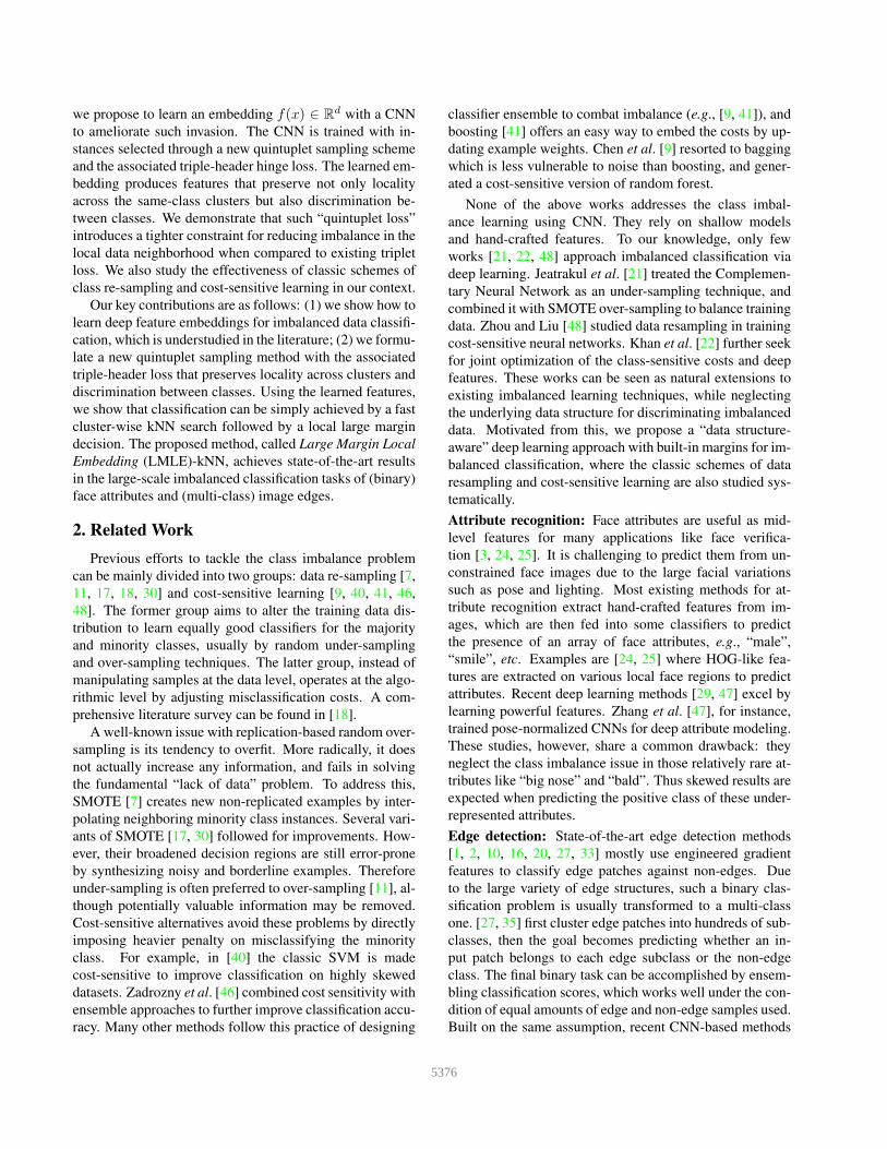
Figure 1. Embeddings by (a) triplet vs. by (b) quintuplet. We exemplify the class imbalance by two different sized classes, where the

clusters are formed by k-means. Our quintuplets enforce both inter-cluster and inter-class margins, while triplets only enforce inter-

class margins irrespective of different class sizes and variations. This difference leads the unique capability of quintuplets in preserving

discrimination in any local neighborhood, and forming a local classification boundary that is insensitive to imbalanced class sizes.

[4, 5, 13, 23, 35, 45] achieve better results by learning deep

features. However, all these methods would face the prob-

lem of data imbalance between each edge subclass and the

dominant non-edge class, which is barely addressed prop-

erly. Only Shen et al. [35] attempt to regularize the multi-

way softmax loss with a balanced weighting between the

“positive” super-class and “negative” class, which is a com-

promise between the binary and multi-class tasks. Here we

propose to explicitly learn discriminative features from im-

balanced data.

3. Learning Deep Representation from Class-

Imbalanced Data

Given an imagery dataset with imbalanced class distribu-

tion, our goal is to learn a Euclidean embedding f(x) from

an image x into a feature space Rd, such that the embed-

ded features are discriminative without any possible local

class imbalance. We constrain this embedding to live on a

d-dimensional hypersphere, i.e., ||f(x)||2 = 1.

3.1. Quintuplet Sampling

To achieve the aforementioned goal, we select quintu-

plets from the imbalanced data as illustrated in Fig. 1. Each

quintuplet is defined as:• xi : an anchor,

• xp+

i : the anchor’s most distant within-cluster neighbor,

• xp−

i : the nearest within-class neighbor of the anchor, but

from a different cluster,

• xp−−

i : the most distant within-class neighbor of the anchor,

• xni : the nearest between-class neighbor of the anchor.

We wish to ensure that the following relationship holds

in the embedding space:

D(f(xi), f(xp+i )) < D(f(xi), f(x

p−i ))

< D(f(xi), f(xp−−i )) < D(f(xi), f(x

ni )), (1)

where D(f(xi), f(xj)) = ‖f(xi) − f(xj)‖22 is the Eu-

clidean distance.

Such a fine-grained similarity defined by quintuplets has

two merits: 1) The ordering in Eq. (1) provides richer in-

formation and a stronger constraint than the conventional

class-level image similarity. In the latter, two images are

considered similar as long as they belong to the same cat-

egory. In contrast, we require two instances to be close at

both class- and cluster-levels to be considered similar. This

actually helps build a local classification boundary with the

most discriminative local samples. Other irrelevant sam-

ples in a class are effectively “ignored” for class separa-

tion, making the local boundary robust and insensitive to

imbalanced class sizes. 2) The quintuplet sampling is re-

peated during CNN training, thus avoiding large informa-

tion loss as in traditional random under-sampling. When

compared with over-sampling strategies, it introduces no

artificial noise. In practice, to ensure adequate learning

for all classes, we collect quintuplets for equal numbers of

minority- and majority-class samples xi in one mini-batch.

Section 5 will quantify the efficacy of this re-sampling

scheme.

Note in the above, we implicitly assume the imbalanced

data are already clustered so that quintuplets can be sam-

pled. In practice, we obtain the initial clusters for each class

by applying k-means on some prior features (e.g., for face

attribute recognition, we employ the pre-trained DeepID2

features [39] on the face verification task). To make the

clustering more robust, an alternating scheme is formu-

lated to refine the clusters using features extracted from the

proposed model itself every 5000 iterations. The overall

pipeline will be summarized in Section 3.2.

3.2. Triple­Header Hinge Loss

To enforce the relationship in Eq. 1 during feature learn-

ing, we apply the large margin idea using the sampled quin-

tuplets. A triple-header hinge loss is formulated to con-

strain three margins between the four distances, and we de-

5377

Training samples

Quintuplet

Mini-batch

...

CNN

CNN

CNN

CNN

CNN

( )

( )

( )

( )

( )

Triple-headerhingeloss

EmbeddingClass 1Cluster1

Cluster2

Class 2

Cluster1

Cluster2

1g

Mini-batchresampling

space2R

3g

...

...2g

Cluster1...

Class c

(a) (b)

CNN

CNN

CNN

CNN

CNN

Trip

le-head

er hin

ge lo

ssMini-

batchesTraining

samples …

EmbeddingQuintuplet

(b)(a)

R2 space

xp−−i

xi

xp+i

xp−i

xni

f(xi)

f(xp+i )

f(xp−i )

f(xp−−i )

f(xni )

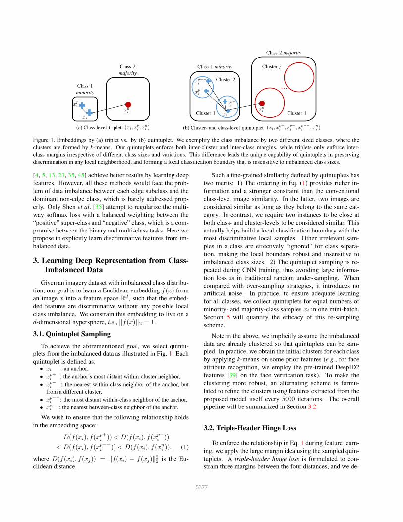
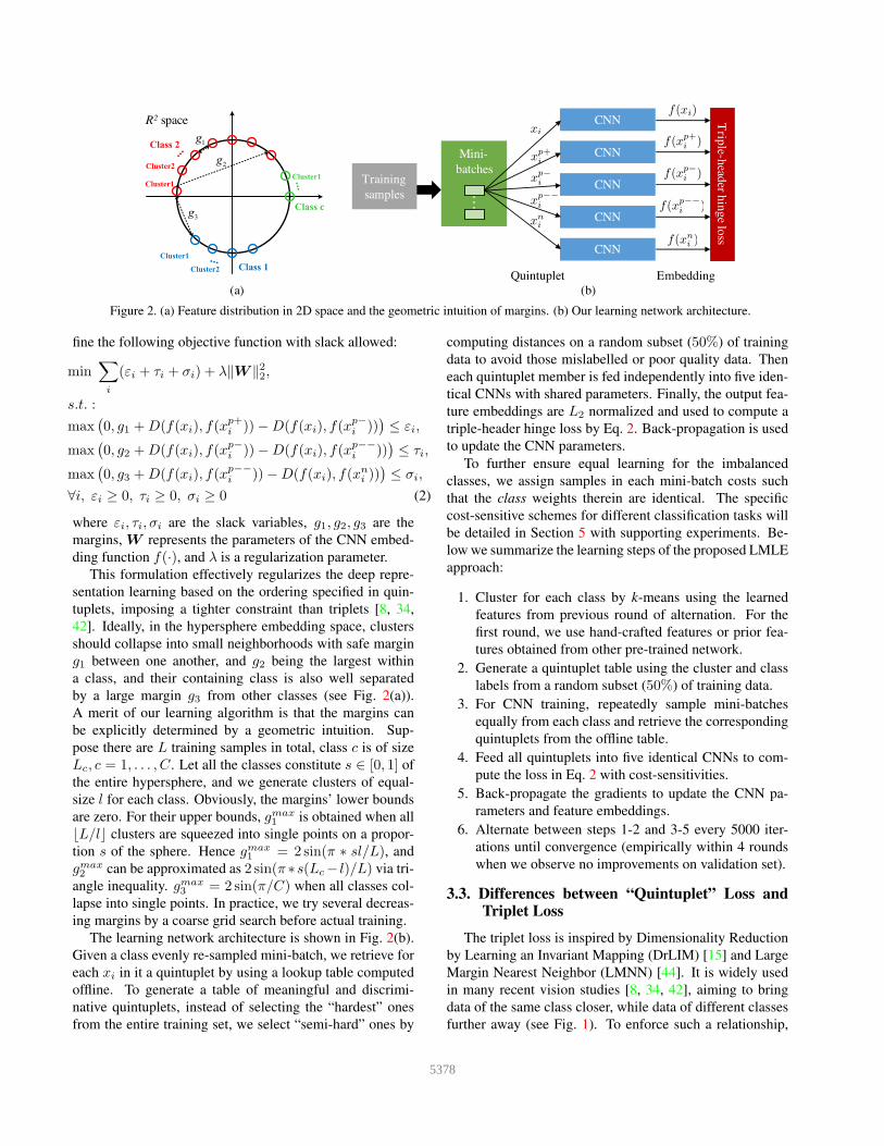
Figure 2. (a) Feature distribution in 2D space and the geometric intuition of margins. (b) Our learning network architecture.

fine the following objective function with slack allowed:

min∑

i

(εi + τi + σi) + λ‖W ‖22,

s.t. :

max(

0, g1 +D(f(xi), f(xp+i ))−D(f(xi), f(x

p−i ))

)

≤ εi,

max(

0, g2 +D(f(xi), f(xp−i ))−D(f(xi), f(x

p−−i ))

)

≤ τi,

max(

0, g3 +D(f(xi), f(xp−−i ))−D(f(xi), f(x

ni ))

)

≤ σi,

∀i, εi ≥ 0, τi ≥ 0, σi ≥ 0 (2)

where εi, τi, σi are the slack variables, g1, g2, g3 are the

margins, W represents the parameters of the CNN embed-

ding function f(·), and λ is a regularization parameter.

This formulation effectively regularizes the deep repre-

sentation learning based on the ordering specified in quin-

tuplets, imposing a tighter constraint than triplets [8, 34,

42]. Ideally, in the hypersphere embedding space, clusters

should collapse into small neighborhoods with safe margin

g1 between one another, and g2 being the largest within

a class, and their containing class is also well separated

by a large margin g3 from other classes (see Fig. 2(a)).

A merit of our learning algorithm is that the margins can

be explicitly determined by a geometric intuition. Sup-

pose there are L training samples in total, class c is of size

Lc, c = 1, . . . , C. Let all the classes constitute s ∈ [0, 1] of

the entire hypersphere, and we generate clusters of equal-

size l for each class. Obviously, the margins’ lower bounds

are zero. For their upper bounds, gmax1 is obtained when all

⌊L/l⌋ clusters are squeezed into single points on a propor-

tion s of the sphere. Hence gmax1 = 2 sin(π ∗ sl/L), and

gmax2 can be approximated as 2 sin(π ∗s(Lc− l)/L) via tri-

angle inequality. gmax3 = 2 sin(π/C) when all classes col-

lapse into single points. In practice, we try several decreas-

ing margins by a coarse grid search before actual training.

The learning network architecture is shown in Fig. 2(b).

Given a class evenly re-sampled mini-batch, we retrieve for

each xi in it a quintuplet by using a lookup table computed

offline. To generate a table of meaningful and discrimi-

native quintuplets, instead of selecting the “hardest” ones

from the entire training set, we select “semi-hard” ones by

computing distances on a random subset (50%) of training

data to avoid those mislabelled or poor quality data. Then

each quintuplet member is fed independently into five iden-

tical CNNs with shared parameters. Finally, the output fea-

ture embeddings are L2 normalized and used to compute a

triple-header hinge loss by Eq. 2. Back-propagation is used

to update the CNN parameters.

To further ensure equal learning for the imbalanced

classes, we assign samples in each mini-batch costs such

that the class weights therein are identical. The specific

cost-sensitive schemes for different classification tasks will

be detailed in Section 5 with supporting experiments. Be-

low we summarize the learning steps of the proposed LMLE

approach:

1. Cluster for each class by k-means using the learned

features from previous round of alternation. For the

first round, we use hand-crafted features or prior fea-

tures obtained from other pre-trained network.

2. Generate a quintuplet table using the cluster and class

labels from a random subset (50%) of training data.

3. For CNN training, repeatedly sample mini-batches

equally from each class and retrieve the corresponding

quintuplets from the offline table.

4. Feed all quintuplets into five identical CNNs to com-

pute the loss in Eq. 2 with cost-sensitivities.

5. Back-propagate the gradients to update the CNN pa-

rameters and feature embeddings.

6. Alternate between steps 1-2 and 3-5 every 5000 iter-

ations until convergence (empirically within 4 rounds

when we observe no improvements on validation set).

3.3. Differences between “Quintuplet” Loss andTriplet Loss

The triplet loss is inspired by Dimensionality Reduction

by Learning an Invariant Mapping (DrLIM) [15] and Large

Margin Nearest Neighbor (LMNN) [44]. It is widely used

in many recent vision studies [8, 34, 42], aiming to bring

data of the same class closer, while data of different classes

further away (see Fig. 1). To enforce such a relationship,

5378

-8 -6 -4 -2 0 2 4 6 8-5

-4

-3

-2

-1

0

1

2

3

4

5

-15 -10 -5 0 5 10-20

-15

-10

-5

0

5

10

15

-10 -8 -6 -4 -2 0 2 4 6 8-8

-6

-4

-2

0

2

4

6

8

NC2NC3NC4NC5PC1PC2

NC1

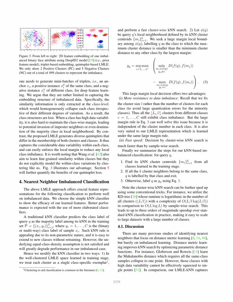
Figure 3. From left to right: 2D feature embedding of one imbal-

anced binary face attribute using DeepID2 model [39] (i.e., prior

feature model), triplet-based embedding, quintuplet-based LMLE.

We only show 2 Positive Clusters (PC) and 5 Negative Clusters

(NC) out of a total of 499 clusters to represent the imbalance.

one needs to generate mini-batches of triplets, i.e., an an-

chor xi, a positive instance xpi of the same class, and a neg-

ative instance xni of different class, for deep feature learn-

ing. We argue that they are rather limited in capturing the

embedding structure of imbalanced data. Specifically, the

similarity information is only extracted at the class-level,

which would homogeneously collapse each class irrespec-

tive of their different degrees of variation. As a result, the

class structures are lost. When a class has high data variabil-

ity, it is also hard to maintain the class-wise margin, leading

to potential invasion of imposter neighbors or even domina-

tion of the majority class in local neighborhood. By con-

trast, the proposed LMLE generates diverse quintuplets that

differ in the membership of both clusters and classes. It thus

captures the considerable data variability within each class,

and can easily enforce the local margin to reduce any local

class imbalance. It is worth noting that Wang et al. [42] also

aim to learn fine-grained similarity within classes but they

do not explicitly model the within-class variations by clus-

tering like us. Fig. 3 illustrates our advantage. Section 5

will further quantify the benefits of our quintuplet loss.

4. Nearest Neighbor Imbalanced Classification

The above LMLE approach offers crucial feature repre-

sentations for the following classification to perform well

on imbalanced data. We choose the simple kNN classifier

to show the efficacy of our learned features. Better perfor-

mance is expected with the use of more elaborated classi-

fiers.

A traditional kNN classifier predicts the class label of

query q as the majority label among its kNN in the training

set P = {(xi, yi)}L

i=1, where yi = 1, . . . , C is the (binary

or multi-way) class label of sample xi. Such kNN rule is

appealing due to its non-parametric nature, and it is easy to

extend to new classes without retraining. However, the un-

derlying equal-class-density assumption is not satisfied and

will greatly degrade performance in our imbalanced case.

Hence we modify the kNN classifier in two ways: 1) In

the well-clustered LMLE space learned in training stage,

we treat each cluster as a single class-specific exemplar2,

2Clustering to aid classification is common in the literature [6, 43].

and perform a fast cluster-wise kNN search. 2) Let φ(q)be query q’s local neighborhood defined by its kNN cluster

centroids {mi}ki=1. We seek a large margin local bound-

ary among φ(q), labelling q as the class to which the max-

imum cluster distance is smaller than the minimum cluster

distance to any other class by the largest margin:

yq = argmaxc=1,...,C

min

mj∈φ(q)yj 6=c

D(f(q), f(mj))

− maxmi∈φ(q)yi=c

D(f(q), f(mi))

. (3)

This large margin local decision offers two advantages:

(i) More resistance to data imbalance: Recall that we fix

the cluster size l rather than the number of clusters for each

class (to avoid large quantization errors for the minority

classes). Thus all the ⌊Lc/l⌋ clusters from different classes

c = 1, . . . , C still exhibit class imbalance. But the large

margin rule in Eq. 3 can well solve this issue because it is

independent of the cluster number in each class. It is also

very suited to our LMLE representation which is learned

under the same large margin rule.

(ii) Fast speed: Decision by cluster-wise kNN search is

much faster than by sample-wise search.

Finally we summarize the steps for our kNN-based im-

balanced classification: for query q,

1. Find its kNN cluster centroids {mi}ki=1 from all

classes learned in the training stage.

2. If all the k cluster neighbors belong to the same class,

q is labelled by that class and exit.

3. Otherwise, label q as yq using Eq. 3.

Note the cluster-wise kNN search can be further sped up

using some conventional tricks. For instance, we utilize the

KD-tree [36] whose runtime is logarithmic in the number of

all clusters (⌊L/l⌋) with a complexity of O(L/l log(L/l))in comparison to O(L logL) by sample-wise search. This

leads to up to three orders of magnitude speedup over stan-

dard kNN classification in practice, making it easy to scale

to large datasets with a large number of classes.

4.1. Discussion

There are many previous studies of identifying nearest

neighbors that focus on distance metric learning [8, 14, 44],

but barely on imbalanced learning. Distance metric learn-

ing improves kNN search by optimizing parametric distance

functions. For instance, Globerson and Roweis [14] learn

the Mahalanobis distance which requires all the same-class

samples collapse to one point. However, those classes with

high data variability cannot be effectively squeezed to sin-

gle points [31]. In comparison, our LMLE-kNN captures

5379

within-class variations across clusters, only which are “col-

lapsed” in the embedding space, thus offering both accuracy

and speed advantages for the kNN search. In [44], the Ma-

halanobis distance is learned to directly improve the large

margin kNN classification, but not under the imbalanced

circumstances. Liu and Chawla [28] provide a weighting

scheme over kNN to correct the classification bias. We “cor-

rect” this bias more effectively by a large margin kNN clas-

sifier with accordingly learned deep features.

5. Results

We study the high-level face attribute classification task

and low-level edge detection task, both with large-scale im-

balanced data. The originally balanced MNIST digit classi-

fication is also studied to experiment with controlled class

imbalance. Our face attribute is binary, with severely imbal-

anced positive and negative samples (e.g., “Bald” attribute:

2% vs. 98%). Our approach predicts 40 attributes simulta-

neously in a multi-task framework. Edge detection is cast as

a multi-class classification problem to address the diversity

of edges, i.e., to predict whether an input image patch be-

longs to any edge class (shape) or the non-edge class. Since

the ultimate goal is still binary, the “positive” edge patches

and “negative” non-edge patches are usually equally sam-

pled for training. Thus severe imbalance exists between the

edge classes (power-law) and dominant non-edge class.

Datasets and evaluation metrics: For face attributes,

we use CelebA dataset [29] that contains 10000 identi-

ties, each with about 20 images. Every face image is an-

notated with 40 attributes and 5 key points to align it to

55× 47 pixels. We partition the dataset following [29]: the

first 160 thousand images (i.e., 8000 identities) for training

(10 thousand images for validation), the following 20 thou-

sand for training SVM classifiers for the PANDA [47] and

ANet [29] methods, and remaining 20 thousand for test-

ing. To account for the imbalanced positive and negative

attribute samples, a balanced accuracy is adopted, that is

accuracy = 0.5(tp/Np+tn/Nn), where Np and Nn are the

numbers of positive and negative samples, while tp and tnare the numbers of true positive and true negative. Note that

this evaluation metric differs from that employed in [29],

where accuracy = ((tp + tn)/(Np + Nn)), which can be

biased to the majority class.

For edge detection, we use the BSDS500 [1] dataset that

contains 200 training, 100 validation and 200 testing im-

ages. We sample 2 million 45 × 45 pixel training patches,

where the numbers of edge and non-edge ones are the same

and there are 150 edge classes formed by k-means. Note

the ultimate goal of edge detection is to produce a full-scale

edge map for one input image, instead of predicting edge

classes for local patches by Eq. 3. To estimate the edge

map in a robust way, we follow [13] to simply transfer and

fuse the overlapping edge label patches of the nearest neigh-

Table 1. Implementation details for the imbalanced classification

tasks considered. For each task, we list its used CNN architecture

(top left), prior features for clustering (top right), and class-specific

cost (bottom).

Face same w.r.t. [39] DeepID2 features in [39]

attributes inv. to class size in batches

same w.r.t. [35] low-level features in [10]Image inv. to class size in batches &edges positive sharing weight [35]

MNIST same w.r.t. [38] pre-trained features by softmax

digits inv. to class size in batches

bors found using our learned representations. After apply-

ing non-maximal suppression, we evaluate edge detection

accuracy by: fixed contour threshold (ODS), per-image best

threshold (OIS), and average precision (AP) [1].

The MNIST experiments are carried out on the challeng-

ing dataset of MNIST-rot-back-image [26]. This extension

dataset contains 28 × 28 digit images with large rotations

and random backgrounds. There are 12000 training images

and 50000 testing images, and we augment the training set

10 times by randomly rotating, mirroring and resizing im-

ages, leaving 10% in it for validation. We report the mean

per-class accuracy in the artificial imbalanced settings.

Parameters: Our CNN is trained using batch size 40,

momentum 0.9, and λ = 0.0005 in Eq. 2. We form clusters

for each class with sizes around l = 200. For those homo-

geneous classes (with only one possible cluster), our within-

class margins actually become nearly zero, which hurts no

performance but only reduces quintuplets to the triplets as

a lower bound baseline. We search k = 20 nearest clus-

ters (i.e., |φ(q)| = 20 in Eq. 3) for querying. Other task-

specific settings are summarized in Table 1. Note the prior

features for clustering are not critical to the final results be-

cause we will gradually learn deep features in alternation

with their clustering every 5000 iterations. Different prior

features generally converge to similar results, but at differ-

ent speeds.

5.1. Comparison with State­of­the­Art Methods

Table 2 compares our LMLE-kNN method for multi-

attribute classification with the state-of-the-art Triplet-

kNN [34], PANDA [47] and ANet [29] methods, which

are trained using the same images and tuned to their best

performance. The attributes and their mean per-class accu-

racies are given in the order of ascending class imbalance

level (= |positive class rate-50|%) to reflect its impact on

performance. It is shown that LMLE-kNN consistently out-

performs other methods across all face attributes, with an

average gap of 4% over the runner-up ANet. Considering

most face attributes exhibit high class imbalance with an

average positive class rate of only 23%, such improvements

are nontrivial and prove our features’ representation power

on imbalanced data. Although the competitive PANDA and

5380

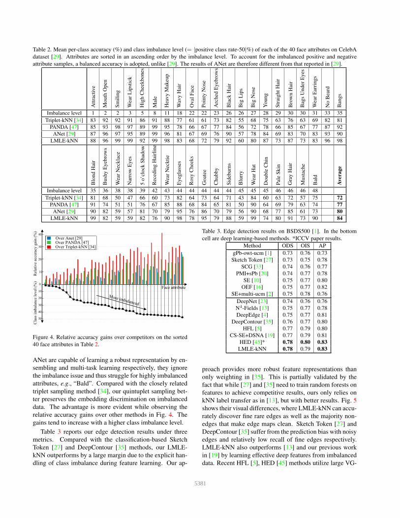
Table 2. Mean per-class accuracy (%) and class imbalance level (= |positive class rate-50|%) of each of the 40 face attributes on CelebA

dataset [29]. Attributes are sorted in an ascending order by the imbalance level. To account for the imbalanced positive and negative

attribute samples, a balanced accuracy is adopted, unlike [29]. The results of ANet are therefore different from that reported in [29].

Att

ract

ive

Mouth

Open

Sm

ilin

g

Wea

rL

ipst

ick

Hig

hC

hee

kbones

Mal

e

Hea

vy

Mak

eup

Wav

yH

air

Oval

Fac

e

Poin

tyN

ose

Arc

hed

Eyeb

row

s

Bla

ckH

air

Big

Lip

s

Big

Nose

Young

Str

aight

Hai

r

Bro

wn

Hai

r

Bag

sU

nder

Eyes

Wea

rE

arri

ngs

No

Bea

rd

Ban

gs

Imbalance level 1 2 2 3 5 8 11 18 22 22 23 26 26 27 28 29 30 30 31 33 35

Triplet-kNN [34] 83 92 92 91 86 91 88 77 61 61 73 82 55 68 75 63 76 63 69 82 81

PANDA [47] 85 93 98 97 89 99 95 78 66 67 77 84 56 72 78 66 85 67 77 87 92

ANet [29] 87 96 97 95 89 99 96 81 67 69 76 90 57 78 84 69 83 70 83 93 90

LMLE-kNN 88 96 99 99 92 99 98 83 68 72 79 92 60 80 87 73 87 73 83 96 98

Blo

nd

Hai

r

Bush

yE

yeb

row

s

Wea

rN

eckla

ce

Nar

row

Eyes

5o’c

lock

Shad

ow

Rec

edin

gH

airl

ine

Wea

rN

eckti

e

Eyeg

lass

es

Rosy

Chee

ks

Goat

ee

Chubby

Sid

eburn

s

Blu

rry

Wea

rH

at

Double

Chin

Pal

eS

kin

Gra

yH

air

Must

ache

Bal

d

Aver

age

Imbalance level 35 36 38 38 39 42 43 44 44 44 44 44 45 45 45 46 46 46 48

Triplet-kNN [34] 81 68 50 47 66 60 73 82 64 73 64 71 43 84 60 63 72 57 75 72

PANDA [47] 91 74 51 51 76 67 85 88 68 84 65 81 50 90 64 69 79 63 74 77

ANet [29] 90 82 59 57 81 70 79 95 76 86 70 79 56 90 68 77 85 61 73 80

LMLE-kNN 99 82 59 59 82 76 90 98 78 95 79 88 59 99 74 80 91 73 90 84

5

10

15

20

0

10

20

30

40

50

Rela

tive

accu

racy

gai

n(%

)Cl

ass i

mba

lanc

e le

vel (

%)

Face attribute

Over PANDA [32]Over Triplet-kNN [22]

More imbalanced

10

20

30

40

0

10

20

30

40

50

Rela

tive

accu

racy

gai

n(%

)Cl

ass i

mba

lanc

e le

vel (

%)

Face attribute

More imbalanced

Over Anet [29]Over PANDA [47]Over Triplet-kNN [34]

Figure 4. Relative accuracy gains over competitors on the sorted

40 face attributes in Table 2.

ANet are capable of learning a robust representation by en-

sembling and multi-task learning respectively, they ignore

the imbalance issue and thus struggle for highly imbalanced

attributes, e.g., “Bald”. Compared with the closely related

triplet sampling method [34], our quintuplet sampling bet-

ter preserves the embedding discrimination on imbalanced

data. The advantage is more evident while observing the

relative accuracy gains over other methods in Fig. 4. The

gains tend to increase with a higher class imbalance level.

Table 3 reports our edge detection results under three

metrics. Compared with the classification-based Sketch

Token [27] and DeepContour [35] methods, our LMLE-

kNN outperforms by a large margin due to the explicit han-

dling of class imbalance during feature learning. Our ap-

Table 3. Edge detection results on BSDS500 [1]. In the bottom

cell are deep learning-based methods. *ICCV paper results.

Method ODS OIS AP

gPb-owt-ucm [1] 0.73 0.76 0.73

Sketch Token [27] 0.73 0.75 0.78

SCG [33] 0.74 0.76 0.77

PMI+sPb [20] 0.74 0.77 0.78

SE [10] 0.75 0.77 0.80

OEF [16] 0.75 0.77 0.82

SE+multi-ucm [2] 0.75 0.78 0.76

DeepNet [23] 0.74 0.76 0.76

N4-Fields [13] 0.75 0.77 0.78

DeepEdge [4] 0.75 0.77 0.81

DeepContour [35] 0.76 0.77 0.80

HFL [5] 0.77 0.79 0.80

CS-SE+DSNA [19] 0.77 0.79 0.81

HED [45]* 0.78 0.80 0.83

LMLE-kNN 0.78 0.79 0.83

proach provides more robust feature representations than

only weighting in [35]. This is partially validated by the

fact that while [27] and [35] need to train random forests on

features to achieve competitive results, ours only relies on

kNN label transfer as in [13], but with better results. Fig. 5

shows their visual differences, where LMLE-kNN can accu-

rately discover fine rare edges as well as the majority non-

edges that make edge maps clean. Sketch Token [27] and

DeepContour [35] suffer from the prediction bias with noisy

edges and relatively low recall of fine edges respectively.

LMLE-kNN also outperforms [13] and our previous work

in [19] by learning effective deep features from imbalanced

data. Recent HFL [5], HED [45] methods utilize large VG-

5381

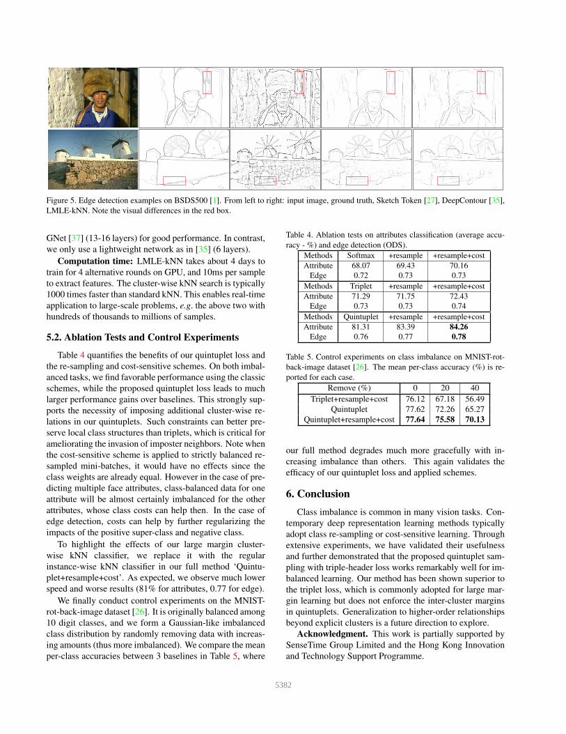
Figure 5. Edge detection examples on BSDS500 [1]. From left to right: input image, ground truth, Sketch Token [27], DeepContour [35],

LMLE-kNN. Note the visual differences in the red box.

GNet [37] (13-16 layers) for good performance. In contrast,

we only use a lightweight network as in [35] (6 layers).

Computation time: LMLE-kNN takes about 4 days to

train for 4 alternative rounds on GPU, and 10ms per sample

to extract features. The cluster-wise kNN search is typically

1000 times faster than standard kNN. This enables real-time

application to large-scale problems, e.g. the above two with

hundreds of thousands to millions of samples.

5.2. Ablation Tests and Control Experiments

Table 4 quantifies the benefits of our quintuplet loss and

the re-sampling and cost-sensitive schemes. On both imbal-

anced tasks, we find favorable performance using the classic

schemes, while the proposed quintuplet loss leads to much

larger performance gains over baselines. This strongly sup-

ports the necessity of imposing additional cluster-wise re-

lations in our quintuplets. Such constraints can better pre-

serve local class structures than triplets, which is critical for

ameliorating the invasion of imposter neighbors. Note when

the cost-sensitive scheme is applied to strictly balanced re-

sampled mini-batches, it would have no effects since the

class weights are already equal. However in the case of pre-

dicting multiple face attributes, class-balanced data for one

attribute will be almost certainly imbalanced for the other

attributes, whose class costs can help then. In the case of

edge detection, costs can help by further regularizing the

impacts of the positive super-class and negative class.

To highlight the effects of our large margin cluster-

wise kNN classifier, we replace it with the regular

instance-wise kNN classifier in our full method ‘Quintu-

plet+resample+cost’. As expected, we observe much lower

speed and worse results (81% for attributes, 0.77 for edge).

We finally conduct control experiments on the MNIST-

rot-back-image dataset [26]. It is originally balanced among

10 digit classes, and we form a Gaussian-like imbalanced

class distribution by randomly removing data with increas-

ing amounts (thus more imbalanced). We compare the mean

per-class accuracies between 3 baselines in Table 5, where

Table 4. Ablation tests on attributes classification (average accu-

racy - %) and edge detection (ODS).

Methods Softmax +resample +resample+cost

Attribute 68.07 69.43 70.16

Edge 0.72 0.73 0.73

Methods Triplet +resample +resample+cost

Attribute 71.29 71.75 72.43

Edge 0.73 0.73 0.74

Methods Quintuplet +resample +resample+cost

Attribute 81.31 83.39 84.26

Edge 0.76 0.77 0.78

Table 5. Control experiments on class imbalance on MNIST-rot-

back-image dataset [26]. The mean per-class accuracy (%) is re-

ported for each case.

Remove (%) 0 20 40

Triplet+resample+cost 76.12 67.18 56.49

Quintuplet 77.62 72.26 65.27

Quintuplet+resample+cost 77.64 75.58 70.13

our full method degrades much more gracefully with in-

creasing imbalance than others. This again validates the

efficacy of our quintuplet loss and applied schemes.

6. Conclusion

Class imbalance is common in many vision tasks. Con-

temporary deep representation learning methods typically

adopt class re-sampling or cost-sensitive learning. Through

extensive experiments, we have validated their usefulness

and further demonstrated that the proposed quintuplet sam-

pling with triple-header loss works remarkably well for im-

balanced learning. Our method has been shown superior to

the triplet loss, which is commonly adopted for large mar-

gin learning but does not enforce the inter-cluster margins

in quintuplets. Generalization to higher-order relationships

beyond explicit clusters is a future direction to explore.

Acknowledgment. This work is partially supported by

SenseTime Group Limited and the Hong Kong Innovation

and Technology Support Programme.

5382

References

[1] P. Arbelaez, M. Maire, C. Fowlkes, and J. Malik. Con-

tour detection and hierarchical image segmentation. TPAMI,

33(5):898–916, 2011.

[2] P. Arbelaez, J. Pont-Tuset, J. Barron, F. Marques, and J. Ma-

lik. Multiscale combinatorial grouping. In CVPR, 2014.

[3] T. Berg and P. N. Belhumeur. POOF: Part-Based One-vs-

One Features for fine-grained categorization, face verifica-

tion, and attribute estimation. In CVPR, 2013.

[4] G. Bertasius, J. Shi, and L. Torresani. Deepedge: A multi-

scale bifurcated deep network for top-down contour detec-

tion. In CVPR, 2015.

[5] G. Bertasius, J. Shi, and L. Torresani. High-for-low and low-

for-high: Efficient boundary detection from deep object fea-

tures and its applications to high-level vision. In ICCV, 2015.

[6] Y.-L. Boureau, N. Le Roux, F. Bach, J. Ponce, and Y. LeCun.

Ask the locals: Multi-way local pooling for image recogni-

tion. In ICCV, 2011.

[7] N. V. Chawla, K. W. Bowyer, L. O. Hall, and W. P.

Kegelmeyer. Smote: synthetic minority over-sampling tech-

nique. JAIR, 16(1):321–357, 2002.

[8] G. Chechik, U. Shalit, V. Sharma, and S. Bengio. An online

algorithm for large scale image similarity learning. In NIPS,

2009.

[9] C. Chen, A. Liaw, and L. Breiman. Using random forest to

learn imbalanced data. Technical report, University of Cali-

fornia, Berkeley, 2004.

[10] P. Dollar and C. L. Zitnick. Fast edge detection using struc-

tured forests. TPAMI, 2015.

[11] C. Drummond and R. C. Holte. C4.5, class imbalance, and

cost sensitivity: Why under-sampling beats over-sampling.

In ICMLW, 2003.

[12] D. Erhan, Y. Bengio, A. Courville, P.-A. Manzagol, P. Vin-

cent, and S. Bengio. Why does unsupervised pre-training

help deep learning? JMLR, 11:625–660, 2010.

[13] Y. Ganin and V. S. Lempitsky. N4-fields: Neural network

nearest neighbor fields for image transforms. In ACCV, 2014.

[14] A. Globerson and S. T. Roweis. Metric learning by collaps-

ing classes. In NIPS, 2006.

[15] R. Hadsell, S. Chopra, and Y. LeCun. Dimensionality reduc-

tion by learning an invariant mapping. In CVPR, 2006.

[16] S. Hallman and C. Fowlkes. Oriented edge forests for bound-

ary detection. In CVPR, 2015.

[17] H. Han, W.-Y. Wang, and B.-H. Mao. Borderline-SMOTE: A

new over-sampling method in imbalanced data sets learning.

In ICIC, 2005.

[18] H. He and E. A. Garcia. Learning from imbalanced data.

TKDE, 21(9):1263–1284, 2009.

[19] C. Huang, C. C. Loy, and X. Tang. Discriminative sparse

neighbor approximation for imbalanced learning. arXiv

preprint, arXiv:1602.01197, 2016.

[20] P. Isola, D. Zoran, D. Krishnan, and E. H. Adelson. Crisp

boundary detection using pointwise mutual information. In

ECCV, 2014.

[21] P. Jeatrakul, K. Wong, and C. Fung. Classification of imbal-

anced data by combining the complementary neural network

and SMOTE algorithm. In ICONIP, 2010.

[22] S. H. Khan, M. Bennamoun, F. Sohel, and R. Togneri. Cost

sensitive learning of deep feature representations from im-

balanced data. arXiv preprint, arXiv:1508.03422v1, 2015.

[23] J. J. Kivinen, C. K. I. Williams, and N. Heess. Visual bound-

ary prediction: A deep neural prediction network and quality

dissection. In AISTATS, 2014.

[24] N. Kumar, A. C. Berg, P. N. Belhumeur, and S. K. Nayar.

Attribute and simile classifiers for face verification. In ICCV,

2009.

[25] N. Kumar, A. C. Berg, P. N. Belhumeur, and S. K. Nayar.

Describable visual attributes for face verification and image

search. TPAMI, 33(10):1962–1977, 2011.

[26] H. Larochelle, D. Erhan, A. Courville, J. Bergstra, and

Y. Bengio. An empirical evaluation of deep architectures on

problems with many factors of variation. In ICML, 2007.

[27] J. Lim, C. L. Zitnick, and P. Dollar. Sketch tokens: A learned

mid-level representation for contour and object detection. In

CVPR, 2013.

[28] W. Liu and S. Chawla. Class confidence weighted kNN al-

gorithms for imbalanced data sets. In PAKDD, 2011.

[29] Z. Liu, P. Luo, X. Wang, and X. Tang. Deep learning face

attributes in the wild. In ICCV, 2015.

[30] T. Maciejewski and J. Stefanowski. Local neighbourhood

extension of SMOTE for mining imbalanced data. In CIDM,

2011.

[31] R. Min, D. A. Stanley, Z. Yuan, A. Bonner, and Z. Zhang. A

deep non-linear feature mapping for large-margin kNN clas-

sification. In ICDM, 2009.

[32] M. Oquab, L. Bottou, I. Laptev, and J. Sivic. Learning and

transferring mid-level image representations using convolu-

tional neural networks. In CVPR, 2014.

[33] X. Ren and L. Bo. Discriminatively Trained Sparse Code

Gradients for Contour Detection. In NIPS, 2012.

[34] F. Schroff, D. Kalenichenko, and J. Philbin. Facenet: A uni-

fied embedding for face recognition and clustering. In CVPR,

2015.

[35] W. Shen, X. Wang, Y. Wang, X. Bai, and Z. Zhang. Deep-

contour: A deep convolutional feature learned by positive-

sharing loss for contour detection. In CVPR, 2015.

[36] C. Silpa-Anan and R. Hartley. Optimised KD-trees for fast

image descriptor matching. In CVPR, 2008.

[37] K. Simonyan and A. Zisserman. Very deep convolutional

networks for large-scale image recognition. In ICLR, 2015.

[38] N. Srivastava and R. R. Salakhutdinov. Discriminative trans-

fer learning with tree-based priors. In NIPS, 2013.

[39] Y. Sun, Y. Chen, X. Wang, and X. Tang. Deep learning face

representation by joint identification-verification. In NIPS,

2014.

[40] Y. Tang, Y.-Q. Zhang, N. Chawla, and S. Krasser. SVMs

modeling for highly imbalanced classification. TSMC,

39(1):281–288, 2009.

[41] K. M. Ting. A comparative study of cost-sensitive boosting

algorithms. In ICML, 2000.

[42] J. Wang, Y. Song, T. Leung, C. Rosenberg, J. Wang,

J. Philbin, B. Chen, and Y. Wu. Learning fine-grained im-

age similarity with deep ranking. In CVPR, 2014.

5383

[43] J. Wang, J. Yang, K. Yu, F. Lv, T. Huang, and Y. Gong.

Locality-constrained linear coding for image classification.

In CVPR, 2010.

[44] K. Q. Weinberger and L. K. Saul. Distance metric learn-

ing for large margin nearest neighbor classification. JMLR,

10:207–244, 2009.

[45] S. Xie and Z. Tu. Holistically-nested edge detection. In

ICCV, 2015.

[46] B. Zadrozny, J. Langford, and N. Abe. Cost-sensitive learn-

ing by cost-proportionate example weighting. In ICDM,

2003.

[47] N. Zhang, M. Paluri, M. Ranzato, T. Darrell, and L. Bourdev.

PANDA: Pose aligned networks for deep attribute modeling.

In CVPR, 2014.

[48] Z.-H. Zhou and X.-Y. Liu. Training cost-sensitive neural net-

works with methods addressing the class imbalance problem.

TKDE, 18(1):63–77, 2006.

5384