Neurocomputing 126 (2014) 15–28

Contents lists available at ScienceDirect

Neurocomputing

0925-23http://d

n CorrE-m

(I. Triguherrera@

journal homepage: www.elsevier.com/locate/neucom

Addressing imbalanced classification with instance generationtechniques: IPADE-ID

Victoria López a,n, Isaac Triguero a, Cristóbal J. Carmona b, Salvador García b,Francisco Herrera a

a Department of Computer Science and Artificial Intelligence, CITIC-UGR (Research Center on Information and Communications Technology),University of Granada, 18071 Granada, Spainb Department of Computer Science, University of Jaén, 23071 Jaén, Spain

a r t i c l e i n f o

Article history:Received 10 May 2012Received in revised form30 November 2012Accepted 10 January 2013Available online 26 July 2013

Keywords:Differential evolutionInstance generationNearest neighborDecision treeImbalanced datasets

12/$ - see front matter & 2013 Elsevier B.V. Ax.doi.org/10.1016/j.neucom.2013.01.050

esponding author. Tel.: +34 958 240598; fax:ail addresses: vlopez@decsai.ugr.es (V. López),ero), ccarmona@ujaen.es (C.J. Carmona), sglodecsai.ugr.es (F. Herrera).

a b s t r a c t

A wide number of real word applications presents a class distribution where examples belonging to oneclass heavily outnumber the examples in the other class. This is an arduous situation where standardclassification techniques usually decrease their performance, creating a handicap to correctly identify theminority class, which is precisely the case under consideration in these applications.

In this work, we propose the usage of the Iterative Instance Adjustment for Imbalanced Domains(IPADE-ID) algorithm. It is an evolutionary framework, which uses an instance generation technique,designed to face the existing imbalance modifying the original training set. The method, iteratively learnsthe appropriate number of examples that represent the classes and their particular positioning. Thelearning process contains three key operations in its design: a customized initialization procedure, anevolutionary optimization of the positioning of the examples and a selection of the most representativeexamples for each class.

An experimental analysis is carried out with a wide range of highly imbalanced datasets over the proposaland recognized solutions to the problem. The results obtained, which have been contrasted through non-parametric statistical tests, show that our proposal outperforms previously proposed methods.

& 2013 Elsevier B.V. All rights reserved.

1. Introduction

Classification with imbalanced datasets is a challenging datamining problem that has attracted a lot of attention in the last years[1,2]. This problem is extremely important since it is predominant inmany real-world data mining applications including, but not limitedto, medical diagnosis, fraud detection, finances, network intrusionand so on. These applications feature samples from one class whichare greatly outnumbered by the samples of the other class. Usually,the minority class is the most interesting class from the learningpoint of view and implies a higher cost of making errors [3,4].

Imbalanced datasets have become an important difficulty tomost classifiers, which assume a nearly balanced class distribu-tion [5]. Standard classifiers are developed to minimize a globalmeasure of error, which is independent of the class distributionand causes a bias towards the majority class, paying less attentionto the minority class. Consequently, classifying the minorityclass is more error prone than classifying the majority class, as ahuge portion of errors are concentrated in the minority class [6].

ll rights reserved.

+34 958 243317.triguero@decsai.ugr.espez@ujaen.es (S. García),

Furthermore, the examples of the minority class can be treated asnoise and they might be completely ignored by the classifier.

Numerous approaches have been suggested to tackle the problemof classification with imbalanced datasets [1,2,7]. These approachesare developed at both data and algorithm levels. Solutions at thealgorithm level modify existing learning algorithms conducting itsoperations on the improvement of the learning on the minority class[8,9]. Solutions at the data level, also known as data sampling, try tomodify the original class distribution in order to obtain a more or lessbalanced dataset that can be used to correctly identify each classwith standard classifiers [10–12].

The use of instance reduction methods [13], which were originallydesigned for other preprocessing purposes (speed up, noise toleranceand reduction of storage requirements of learning methods [14]), canalso be applied to imbalanced datasets [15,16] as a data level solutionthat is used to find a balance between the minority and the majorityclasses. It is important that instance reduction methods adapt theirbias to this situation to obtain high performances.

An instance reduction process is devoted to find the bestreduced set that represents the original training data with a lessernumber of instances. This methodology can be divided intoInstance Selection (IS) [13,17,18] and Instance Generation (IG)depending on how it creates the reduced set [19,20]. The formerprocess attempts to choose an appropriate subset of the original

V. López et al. / Neurocomputing 126 (2014) 15–2816

training data, while the latter can also build new artificialinstances to better adjust the decision boundaries of the classes.In this manner, the IG process fills some regions in the domainof the problem, which have no representative examples in theoriginal dataset. IS methods have been applied to imbalanceddatasets with promising results [15,16,21], however, to the best ofour knowledge, IG techniques have not been used yet to deal withimbalanced classification problems.

Following the idea of IG techniques, we propose the usage of theIterative Instance Adjustment for Imbalanced Domains (IPADE-ID)algorithm to deal with highly imbalanced datasets. IPADE-ID is amethod inspired by the IG technique IPADE [22,23], that tries toobtain an adequate synthetic training set from the original trainingset following an incremental approach to determine the mostappropriate number of instances per class. The proposal is based inthree fundamental operations: a customized initialization procedure,an evolutionary adjustment of the prototypes and the selection of themost representative examples to define the classes. The initializationprocedure should be befitting to the specific learning algorithm usedwith IPADE-ID.

In this work, we choose the Nearest Neighbor (NN) rule [24]and the C4.5 algorithm [25] as learning methods. In this way,we provide suitable initialization procedures for IPADE-ID thatmatches these learning approaches. At each step, an optimizationprocedure, based on an adaptive differential evolution algorithm[26–28], adjusts the positioning of the instances generated up tonow, and a selection procedure adds new instances if needed. Thisselection procedure has been particularly designed to considerthe existing imbalanced scenario focusing on the performance ofthe minority class. This informed and organized combinationof techniques, leads us to a hybrid artificial intelligent system[29,30] that is able to cope with imbalanced datasets.

In order to analyze the performance of the proposal, we focuson highly imbalanced binary classification problems, havingselected a benchmark of 44 problems from KEEL dataset reposi-tory1 [31]. We will perform our experimental analysis focusing onthe precision of the models using the Area Under the ROC curve(AUC) [32]. This study will be carried out using non-parametricstatistical tests to check whether there are significant differencesamong the results [33,34].

The rest of the paper is organized as follows. In Section 2, somebackground about classification with imbalanced datasets andinstance generation techniques is given. Next, Section 3 introducesthe proposed approach. Sections 4 and 5 describe the experimentalframework used and the analysis of results, respectively. Finally, theconclusions achieved in this work are shown in Section 6.

2. Background

This section purpose is to provide the background informationneeded to describe our proposal. It is divided in two parts: adescription of instance generation techniques (Section 2.1) andan introduction to the problem of classification with imbalanceddatasets (Section 2.2).

2.1. Instance generation techniques

This section presents the definition and notation for instancegeneration techniques.

A formal specification of the instance generation problem is thefollowing: Let xp be an example where xp ¼ ðxp1; xp2;…; xpD;CpÞ,with xp belonging to a class Ci given by Cp and a D-dimensional

1 http://www.keel.es/datasets.php.

space in which xpj is the value of the j-th feature of the p-thsample. Then, let us assume that there is a training set TR whichconsists of n instances xp and a test set TS composed of t instancesxq, with Cq unknown.

The original purpose of IG is to obtain an instance generated set(GS), which consists of r, ron, instances pu where pu ¼ ðpu1;pu2;…; puD;CuÞ, which are either selected or generated from theexamples of TR. The instances of the generated set are determinedto efficiently represent the distributions of the classes and todiscriminate well when used to classify the training objects.

This methodology, also known as instance abstraction, hasbeen widely studied in the specialized literature focusing on theNN rule [24] as target classifier. These techniques follow multiplemechanisms to generate an appropriate GS, such as interpolationsbetween instances, movements of instances and artificial genera-tion of new data. Using the taxonomy proposed in [20], they canbe divided into several families depending on the main heuristicoperation: positioning adjustment [35], class re-labeling [36],centroid-based [19] and space-splitting [37].

Among these families of methods, the algorithms that arebased on the adjustment of the position of the instances werehighlighted as outstanding methods in [20]. This methodologycan be viewed as an optimization process of the positioning ofthe instances [38]. The precursor algorithm of this family is thelearning vector quantization proposed by Kohonen [39]. One of themost recent and promising algorithms is the model presented in[22], called IPADE, which follows an incremental addition processof instances to determine which classes need more instances to berepresented and their best locations.

More information about instance generation approaches (andinstance reduction approaches in general) can be found at the SCI2Sthematic public website on Prototype Reduction in Nearest NeighborClassification: Prototype Selection and Prototype Generation.2

2.2. Imbalanced datasets in classification

In this section we delimit the context in which this work iscontent, briefly introducing the problem of imbalanced classifica-tion. Then, we will describe which approaches are used to deal withthis problem, giving special importance to data level approachesthat modify the class distribution. We finish this section describingthe evaluation metrics that are used in this specific problem withrespect to the most common ones in classification.

2.2.1. The problem of imbalanced datasetsIn some classification problems, the number of instances that

belong to each class is radically different [1,2]. The problem ofclassification with imbalanced datasets has acquired much rele-vance in the last time due to its presence in abundant real-worldapplications such as medical diagnosis [40], finances [41,42],anomaly detection [43] or bioinformatics [44] just naming someof them. Furthermore, the underrepresented class is usually themost interesting class from the learning point of view incorporat-ing high costs when it is not correctly identified [3,4].

In this paper, we focus on two-class imbalanced datasets,where there is a positive (minority) class, with the lowest numberof instances, and a negative (majority) class, with the highestnumber of instances. Although this class distribution is frequent inreal data mining problems, standard classifiers are not usually ableto cope with the correct identification of positive samples. Fre-quently, standard classifiers are biased towards the majority classas they are guided by global performance measures, selectingmore general rules that cover as many samples as possible and

2 http://sci2s.ugr.es/pr/.

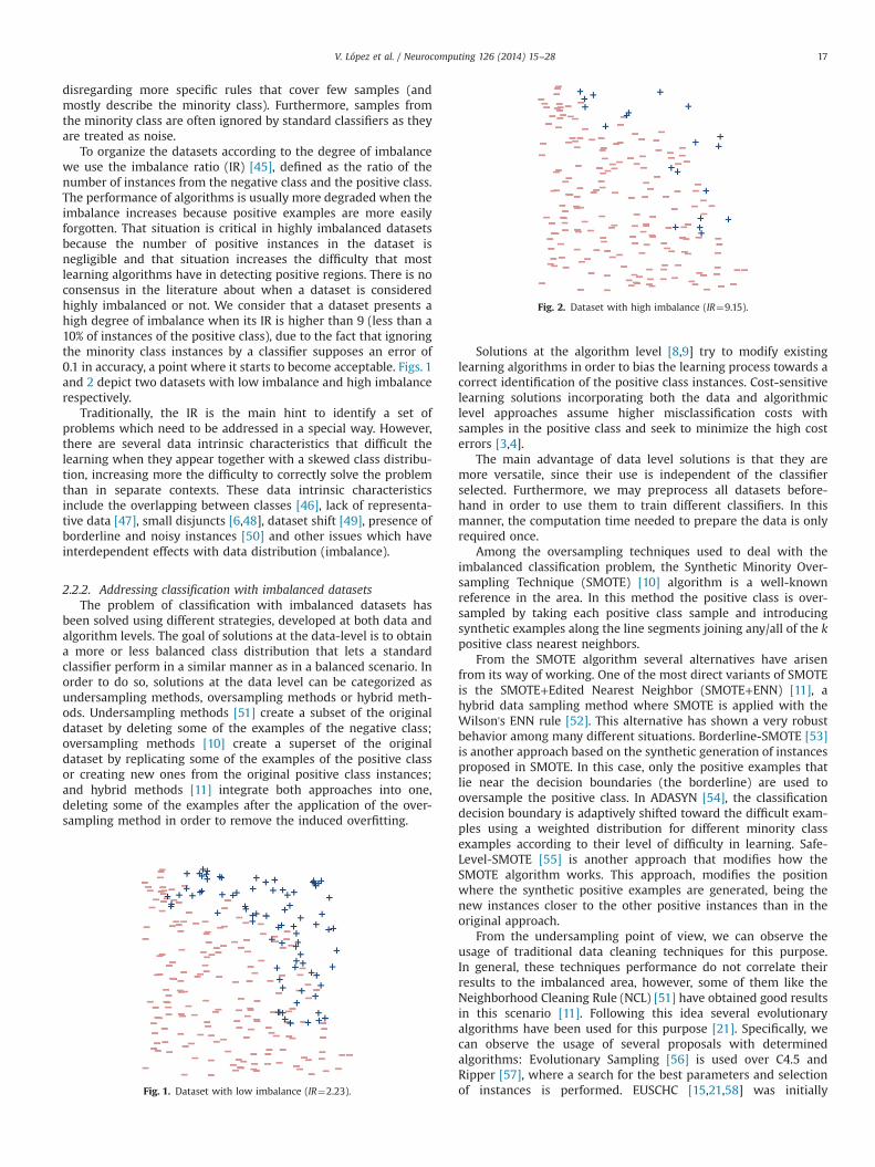
Fig. 2. Dataset with high imbalance (IR¼9.15).

V. López et al. / Neurocomputing 126 (2014) 15–28 17

disregarding more specific rules that cover few samples (andmostly describe the minority class). Furthermore, samples fromthe minority class are often ignored by standard classifiers as theyare treated as noise.

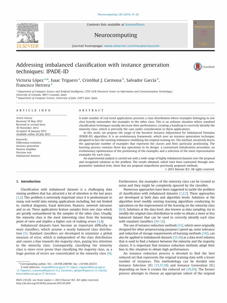
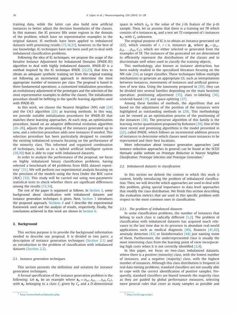
To organize the datasets according to the degree of imbalancewe use the imbalance ratio (IR) [45], defined as the ratio of thenumber of instances from the negative class and the positive class.The performance of algorithms is usually more degraded when theimbalance increases because positive examples are more easilyforgotten. That situation is critical in highly imbalanced datasetsbecause the number of positive instances in the dataset isnegligible and that situation increases the difficulty that mostlearning algorithms have in detecting positive regions. There is noconsensus in the literature about when a dataset is consideredhighly imbalanced or not. We consider that a dataset presents ahigh degree of imbalance when its IR is higher than 9 (less than a10% of instances of the positive class), due to the fact that ignoringthe minority class instances by a classifier supposes an error of0.1 in accuracy, a point where it starts to become acceptable. Figs. 1and 2 depict two datasets with low imbalance and high imbalancerespectively.

Traditionally, the IR is the main hint to identify a set ofproblems which need to be addressed in a special way. However,there are several data intrinsic characteristics that difficult thelearning when they appear together with a skewed class distribu-tion, increasing more the difficulty to correctly solve the problemthan in separate contexts. These data intrinsic characteristicsinclude the overlapping between classes [46], lack of representa-tive data [47], small disjuncts [6,48], dataset shift [49], presence ofborderline and noisy instances [50] and other issues which haveinterdependent effects with data distribution (imbalance).

2.2.2. Addressing classification with imbalanced datasetsThe problem of classification with imbalanced datasets has

been solved using different strategies, developed at both data andalgorithm levels. The goal of solutions at the data-level is to obtaina more or less balanced class distribution that lets a standardclassifier perform in a similar manner as in a balanced scenario. Inorder to do so, solutions at the data level can be categorized asundersampling methods, oversampling methods or hybrid meth-ods. Undersampling methods [51] create a subset of the originaldataset by deleting some of the examples of the negative class;oversampling methods [10] create a superset of the originaldataset by replicating some of the examples of the positive classor creating new ones from the original positive class instances;and hybrid methods [11] integrate both approaches into one,deleting some of the examples after the application of the over-sampling method in order to remove the induced overfitting.

Fig. 1. Dataset with low imbalance (IR¼2.23).

Solutions at the algorithm level [8,9] try to modify existinglearning algorithms in order to bias the learning process towards acorrect identification of the positive class instances. Cost-sensitivelearning solutions incorporating both the data and algorithmiclevel approaches assume higher misclassification costs withsamples in the positive class and seek to minimize the high costerrors [3,4].

The main advantage of data level solutions is that they aremore versatile, since their use is independent of the classifierselected. Furthermore, we may preprocess all datasets before-hand in order to use them to train different classifiers. In thismanner, the computation time needed to prepare the data is onlyrequired once.

Among the oversampling techniques used to deal with theimbalanced classification problem, the Synthetic Minority Over-sampling Technique (SMOTE) [10] algorithm is a well-knownreference in the area. In this method the positive class is over-sampled by taking each positive class sample and introducingsynthetic examples along the line segments joining any/all of the kpositive class nearest neighbors.

From the SMOTE algorithm several alternatives have arisenfrom its way of working. One of the most direct variants of SMOTEis the SMOTE+Edited Nearest Neighbor (SMOTE+ENN) [11], ahybrid data sampling method where SMOTE is applied with theWilson's ENN rule [52]. This alternative has shown a very robustbehavior among many different situations. Borderline-SMOTE [53]is another approach based on the synthetic generation of instancesproposed in SMOTE. In this case, only the positive examples thatlie near the decision boundaries (the borderline) are used tooversample the positive class. In ADASYN [54], the classificationdecision boundary is adaptively shifted toward the difficult exam-ples using a weighted distribution for different minority classexamples according to their level of difficulty in learning. Safe-Level-SMOTE [55] is another approach that modifies how theSMOTE algorithm works. This approach, modifies the positionwhere the synthetic positive examples are generated, being thenew instances closer to the other positive instances than in theoriginal approach.

From the undersampling point of view, we can observe theusage of traditional data cleaning techniques for this purpose.In general, these techniques performance do not correlate theirresults to the imbalanced area, however, some of them like theNeighborhood Cleaning Rule (NCL) [51] have obtained good resultsin this scenario [11]. Following this idea several evolutionaryalgorithms have been used for this purpose [21]. Specifically, wecan observe the usage of several proposals with determinedalgorithms: Evolutionary Sampling [56] is used over C4.5 andRipper [57], where a search for the best parameters and selectionof instances is performed. EUSCHC [15,21,58] was initially

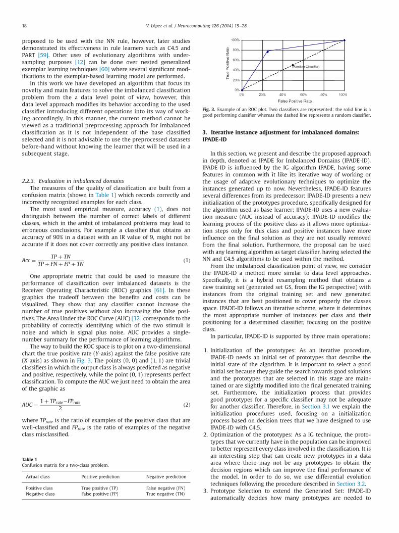
Fig. 3. Example of an ROC plot. Two classifiers are represented: the solid line is agood performing classifier whereas the dashed line represents a random classifier.

V. López et al. / Neurocomputing 126 (2014) 15–2818

proposed to be used with the NN rule, however, later studiesdemonstrated its effectiveness in rule learners such as C4.5 andPART [59]. Other uses of evolutionary algorithms with under-sampling purposes [12] can be done over nested generalizedexemplar learning techniques [60] where several significant mod-ifications to the exemplar-based learning model are performed.

In this work we have developed an algorithm that focus itsnovelty and main features to solve the imbalanced classificationproblem from the a data level point of view, however, thisdata level approach modifies its behavior according to the usedclassifier introducing different operations into its way of work-ing accordingly. In this manner, the current method cannot beviewed as a traditional preprocessing approach for imbalancedclassification as it is not independent of the base classifiedselected and it is not advisable to use the preprocessed datasetsbefore-hand without knowing the learner that will be used in asubsequent stage.

2.2.3. Evaluation in imbalanced domainsThe measures of the quality of classification are built from a

confusion matrix (shown in Table 1) which records correctly andincorrectly recognized examples for each class.

The most used empirical measure, accuracy (1), does notdistinguish between the number of correct labels of differentclasses, which in the ambit of imbalanced problems may lead toerroneous conclusions. For example a classifier that obtains anaccuracy of 90% in a dataset with an IR value of 9, might not beaccurate if it does not cover correctly any positive class instance.

Acc¼ TP þ TNTP þ FN þ FP þ TN

ð1Þ

One appropriate metric that could be used to measure theperformance of classification over imbalanced datasets is theReceiver Operating Characteristic (ROC) graphics [61]. In thesegraphics the tradeoff between the benefits and costs can bevisualized. They show that any classifier cannot increase thenumber of true positives without also increasing the false posi-tives. The Area Under the ROC Curve (AUC) [32] corresponds to theprobability of correctly identifying which of the two stimuli isnoise and which is signal plus noise. AUC provides a single-number summary for the performance of learning algorithms.

The way to build the ROC space is to plot on a two-dimensionalchart the true positive rate (Y-axis) against the false positive rate(X-axis) as shown in Fig. 3. The points (0, 0) and (1, 1) are trivialclassifiers in which the output class is always predicted as negativeand positive, respectively, while the point (0, 1) represents perfectclassification. To compute the AUC we just need to obtain the areaof the graphic as

AUC ¼ 1þ TPrate�FPrate

2ð2Þ

where TPrate is the ratio of examples of the positive class that arewell-classified and FPrate is the ratio of examples of the negativeclass misclassified.

Table 1Confusion matrix for a two-class problem.

Actual class Positive prediction Negative prediction

Positive class True positive (TP) False negative (FN)Negative class False positive (FP) True negative (TN)

3. Iterative instance adjustment for imbalanced domains:IPADE-ID

In this section, we present and describe the proposed approachin depth, denoted as IPADE for Imbalanced Domains (IPADE-ID).IPADE-ID is influenced by the IG algorithm IPADE, having somefeatures in common with it like its iterative way of working orthe usage of adaptive evolutionary techniques to optimize theinstances generated up to now. Nevertheless, IPADE-ID featuresseveral differences from its predecessor: IPADE-ID presents a newinitialization of the prototypes procedure, specifically designed forthe algorithm used as base learner; IPADE-ID uses a new evalua-tion measure (AUC instead of accuracy); IPADE-ID modifies thelearning process of the positive class as it allows more optimiza-tion steps only for this class and positive instances have moreinfluence on the final solution as they are not usually removedfrom the final solution. Furthermore, the proposal can be usedwith any learning algorithm as target classifier, having selected theNN and C4.5 algorithms to be used within the method.

From the imbalanced classification point of view, we considerthe IPADE-ID a method more similar to data level approaches.Specifically, it is a hybrid resampling method that obtains anew training set (generated set GS, from the IG perspective) withinstances from the original training set and new generatedinstances that are best positioned to cover properly the classesspace. IPADE-ID follows an iterative scheme, where it determinesthe most appropriate number of instances per class and theirpositioning for a determined classifier, focusing on the positiveclass.

In particular, IPADE-ID is supported by three main operations:

1.

Initialization of the prototypes: As an iterative procedure,IPADE-ID needs an initial set of prototypes that describe theinitial state of the algorithm. It is important to select a goodinitial set because they guide the search towards good solutionsand the prototypes that are selected in this stage are main-tained or are slightly modified into the final generated trainingset. Furthermore, the initialization process that providesgood prototypes for a specific classifier may not be adequatefor another classifier. Therefore, in Section 3.1 we explain theinitialization procedures used, focusing on a initializationprocess based on decision trees that we have designed to useIPADE-ID with C4.5.

2.

Optimization of the prototypes: As a IG technique, the proto-types that we currently have in the population can be improvedto better represent every class involved in the classification. It isan interesting step that can create new prototypes in a dataarea where there may not be any prototypes to obtain thedecision regions which can improve the final performance ofthe model. In order to do so, we use differential evolutiontechniques following the procedure described in Section 3.2.

3.

Prototype Selection to extend the Generated Set: IPADE-IDautomatically decides how many prototypes are needed to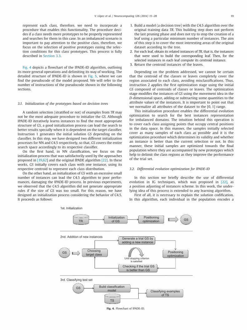

V. López et al. / Neurocomputing 126 (2014) 15–28 19

represent each class, therefore, we need to incorporate aprocedure that enables this functionality. The procedure deci-des if a class needs more prototypes to be properly representedand searches for them in this case. In an imbalanced scenario isimportant to pay attention to the positive class, therefore, wefocus on the selection of positive prototypes easing the selec-tion conditions for this class prototypes. This process is fullydescribed in Section 3.3.

Fig. 4 depicts a flowchart of the IPADE-ID algorithm, outliningits more general operations and delimiting its way of working. Thedetailed structure of IPADE-ID is shown in Fig. 5, where we canfind the pseudocode of the model proposed. We will refer to thenumber of instructions of the pseudocode shown in the followingsections.

3.1. Initialization of the prototypes based on decision trees

A random selection (stratified or not) of examples from TR maynot be the most adequate procedure to initialize the GS. AlthoughIPADE-ID iteratively learns instances to find the most appropriatestructure of GS, a good initialization process can lead the search tobetter results specially when it is dependent on the target classifier.Instruction 1 generates the initial solution GS depending on theclassifier. In this step, we have designed two different initializationprocesses for NN and C4.5 respectively, so that, GS covers the entiresearch space accordingly to its respective classifier.

On the first hand, in NN classification, we focus on theinitialization process that was satisfactorily used by the approachesproposed in [19,62] and the original IPADE algorithm [22]. In theseworks, GS initially covers each class with one instance, using itsrespective centroid to represent each class distribution.

On the other hand, an initialization of GSwith an excessive smallnumber of instances can lead the C4.5 algorithm to poor perfor-mances, damaging the IPADE-ID process. In previous experiments,we observed that the C4.5 algorithm did not generate appropriaterules if the size of GS was too small. For this reason, we havedesigned an initialization process considering the behavior of C4.5.It proceeds as follows:

TRInitialization

of GS

Choosingtarget class

2nd. Addition of new instances

3rd. Classifying test set

Geneaddin

Cheis

Build classificationmodel

Unt

GS

GS

TS

1st. Initialization

Fig. 4. Flowchart

1.

rateg a

ckin bet

il stois s

of I

Build a model (a decision tree) with the C4.5 algorithm over theoriginal training data TR. This building step does not performthe last pruning phase and does not try to stop the creation of aleaf using a particular minimum number of instances. The aimof this step is to cover the most interesting areas of the originaldataset according to the tree.

2.

For each leaf, obtain its related instances of TR, that is, the instancesthat were used to build the corresponding leaf. Then, for theselected instances in each leaf compute its centroid instance.

3.

Return the centroid instances of the leaves.

Depending on the problem addressed, we cannot be certainthat the centroid of the classes or leaves completely cover theregion associated to each class, avoiding misclassifications. Thus,instruction 2 applies the first optimization stage using the initialGS composed of centroids of classes or leaves. The optimizationstage modifies the instances of GS using the movement idea in theD-dimensional space, adding or subtracting some quantities to theattribute values of the instances. It is important to point out thatwe normalize all attributes of the dataset to the [0, 1] range.

This initialization procedure enables the differential evolutionoptimization to search for the best instances representationfor imbalanced domains. The intuition behind this operation isto cover each class assigning points that occupy central positionsin the data space. In this manner, the samples initially selectedcover as many samples of each class as possible and it is theoptimization procedure which determines its validity and whetheran instance is better than the current selection or not. In thismanner, these initial samples are optimized towards the finalpopulation where they are accompanied by new prototypes whichhelp to delimit the class regions as they improve the performanceof the trial set.

3.2. Differential evolution optimization for IPADE-ID

In this section we briefly describe the use of differentialevolution in IG techniques, which was proposed in [22], asa position adjusting of instances scheme. In this work, the under-lying idea of this process is extended to any learning algorithm.

First of all, it is necessary to explain the solution codification.In this algorithm, each individual in the population encodes a

Positioningoptimization

a trial GS by new instance

Positioningoptimization

g if the trial GSter than GS

pping criterionatisfied

GS

Classifying examplesof TS

PADE-ID.

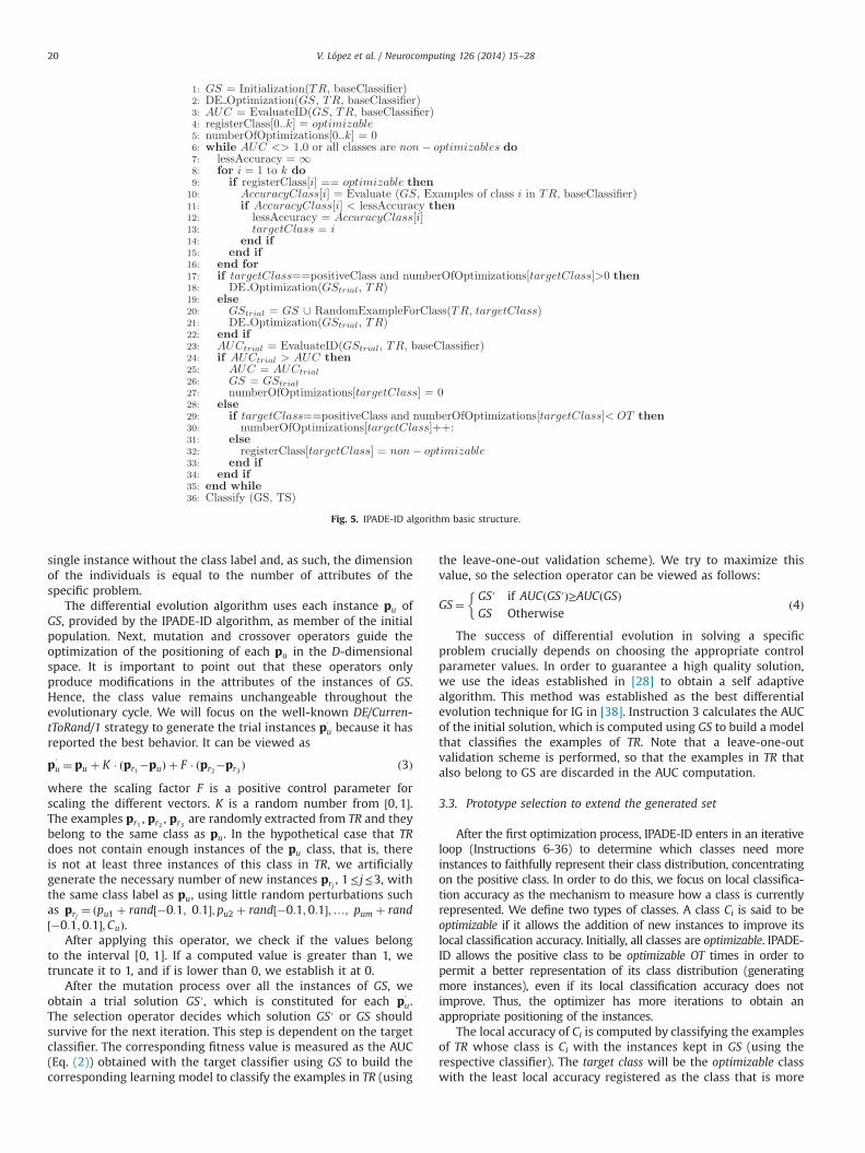
Fig. 5. IPADE-ID algorithm basic structure.

V. López et al. / Neurocomputing 126 (2014) 15–2820

single instance without the class label and, as such, the dimensionof the individuals is equal to the number of attributes of thespecific problem.

The differential evolution algorithm uses each instance pu ofGS, provided by the IPADE-ID algorithm, as member of the initialpopulation. Next, mutation and crossover operators guide theoptimization of the positioning of each pu in the D-dimensionalspace. It is important to point out that these operators onlyproduce modifications in the attributes of the instances of GS.Hence, the class value remains unchangeable throughout theevolutionary cycle. We will focus on the well-known DE/Curren-tToRand/1 strategy to generate the trial instances p′

u because it hasreported the best behavior. It can be viewed as

p′u ¼ pu þ K � ðpr1�puÞ þ F � ðpr2�pr3 Þ ð3Þ

where the scaling factor F is a positive control parameter forscaling the different vectors. K is a random number from ½0;1�.The examples pr1 , pr2 , pr3 are randomly extracted from TR and theybelong to the same class as pu. In the hypothetical case that TRdoes not contain enough instances of the pu class, that is, thereis not at least three instances of this class in TR, we artificiallygenerate the necessary number of new instances prj , 1≤ j≤3, withthe same class label as pu, using little random perturbations suchas prj ¼ ðpu1 þ rand½�0:1; 0:1�; pu2 þ rand½�0:1;0:1�;…; pum þ rand½�0:1;0:1�;CuÞ.

After applying this operator, we check if the values belongto the interval [0, 1]. If a computed value is greater than 1, wetruncate it to 1, and if is lower than 0, we establish it at 0.

After the mutation process over all the instances of GS, weobtain a trial solution GS′, which is constituted for each p′

u.The selection operator decides which solution GS′ or GS shouldsurvive for the next iteration. This step is dependent on the targetclassifier. The corresponding fitness value is measured as the AUC(Eq. (2)) obtained with the target classifier using GS to build thecorresponding learning model to classify the examples in TR (using

the leave-one-out validation scheme). We try to maximize thisvalue, so the selection operator can be viewed as follows:

GS¼ GS′ if AUCðGS′Þ≥AUCðGSÞGS Otherwise

�ð4Þ

The success of differential evolution in solving a specificproblem crucially depends on choosing the appropriate controlparameter values. In order to guarantee a high quality solution,we use the ideas established in [28] to obtain a self adaptivealgorithm. This method was established as the best differentialevolution technique for IG in [38]. Instruction 3 calculates the AUCof the initial solution, which is computed using GS to build a modelthat classifies the examples of TR. Note that a leave-one-outvalidation scheme is performed, so that the examples in TR thatalso belong to GS are discarded in the AUC computation.

3.3. Prototype selection to extend the generated set

After the first optimization process, IPADE-ID enters in an iterativeloop (Instructions 6-36) to determine which classes need moreinstances to faithfully represent their class distribution, concentratingon the positive class. In order to do this, we focus on local classifica-tion accuracy as the mechanism to measure how a class is currentlyrepresented. We define two types of classes. A class Ci is said to beoptimizable if it allows the addition of new instances to improve itslocal classification accuracy. Initially, all classes are optimizable. IPADE-ID allows the positive class to be optimizable OT times in order topermit a better representation of its class distribution (generatingmore instances), even if its local classification accuracy does notimprove. Thus, the optimizer has more iterations to obtain anappropriate positioning of the instances.

The local accuracy of Ci is computed by classifying the examplesof TR whose class is Ci with the instances kept in GS (using therespective classifier). The target class will be the optimizable classwith the least local accuracy registered as the class that is more

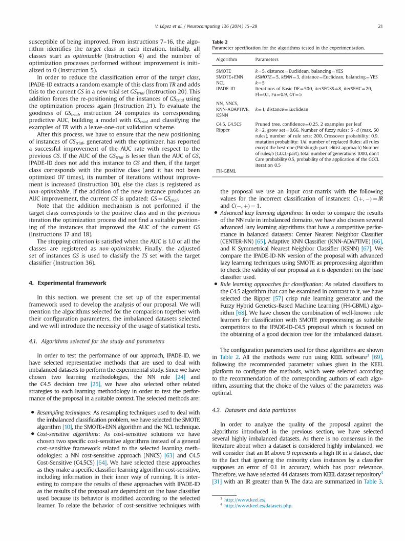
Table 2Parameter specification for the algorithms tested in the experimentation.

Algorithm Parameters

SMOTE k¼5, distance¼Euclidean, balancing¼YESSMOTE+ENN kSMOTE¼5, kENN¼3, distance¼Euclidean, balancing¼YESNCL k¼5IPADE-ID Iterations of Basic DE¼500, iterSFGSS¼8, iterSFHC¼20,

Fl¼0.1, Fu¼0.9, OT¼5

NN, NNCS,KNN-ADAPTIVE,KSNN

k¼1, distance¼Euclidean

C4.5, C4.5CS Pruned tree, confidence¼0.25, 2 examples per leafRipper k¼2, grow set¼0.66, Number of fuzzy rules: 5 � d (max. 50

rules), number of rule sets: 200, Crossover probability: 0.9,mutation probability: 1/d, number of replaced Rules: all rulesexcept the best-one (Pittsburgh-part, elitist approach) Numberof rules/5 (GCCL-part), total number of generations 1000, don'tCare probability 0.5, probability of the application of the GCCLiteration 0.5

FH-GBML

V. López et al. / Neurocomputing 126 (2014) 15–28 21

susceptible of being improved. From instructions 7–16, the algo-rithm identifies the target class in each iteration. Initially, allclasses start as optimizable (Instruction 4) and the number ofoptimization processes performed without improvement is initi-alized to 0 (Instruction 5).

In order to reduce the classification error of the target class,IPADE-ID extracts a random example of this class from TR and addsthis to the current GS in a new trial set GStrial (Instruction 20). Thisaddition forces the re-positioning of the instances of GStrial usingthe optimization process again (Instruction 21). To evaluate thegoodness of GStrial, instruction 24 computes its correspondingpredictive AUC, building a model with GStrial and classifying theexamples of TR with a leave-one-out validation scheme.

After this process, we have to ensure that the new positioningof instances of GStrial, generated with the optimizer, has reporteda successful improvement of the AUC rate with respect to theprevious GS. If the AUC of the GStrial is lesser than the AUC of GS,IPADE-ID does not add this instance to GS and then, if the targetclass corresponds with the positive class (and it has not beenoptimized OT times), its number of iterations without improve-ment is increased (Instruction 30), else the class is registered asnon-optimizable. If the addition of the new instance produces anAUC improvement, the current GS is updated: GS¼ GStrial.

Note that the addition mechanism is not performed if thetarget class corresponds to the positive class and in the previousiteration the optimization process did not find a suitable position-ing of the instances that improved the AUC of the current GS(Instructions 17 and 18).

The stopping criterion is satisfied when the AUC is 1.0 or all theclasses are registered as non-optimizable. Finally, the adjustedset of instances GS is used to classify the TS set with the targetclassifier (Instruction 36).

4. Experimental framework

In this section, we present the set up of the experimentalframework used to develop the analysis of our proposal. We willmention the algorithms selected for the comparison together withtheir configuration parameters, the imbalanced datasets selectedand we will introduce the necessity of the usage of statistical tests.

4.1. Algorithms selected for the study and parameters

In order to test the performance of our approach, IPADE-ID, wehave selected representative methods that are used to deal withimbalanced datasets to perform the experimental study. Since we havechosen two learning methodologies, the NN rule [24] andthe C4.5 decision tree [25], we have also selected other relatedstrategies to each learning methodology in order to test the perfor-mance of the proposal in a suitable context. The selected methods are:

�

Resampling techniques: As resampling techniques used to deal withthe imbalanced classification problem, we have selected the SMOTEalgorithm [10], the SMOTE+ENN algorithm and the NCL technique.

�

3 http://www.keel.es/.4 http://www.keel.es/datasets.php.

Cost-sensitive algorithms: As cost-sensitive solutions we havechosen two specific cost-sensitive algorithms instead of a generalcost-sensitive framework related to the selected learning meth-odologies: a NN cost-sensitive approach (NNCS) [63] and C4.5Cost-Sensitive (C4.5CS) [64]. We have selected these approachesas they make a specific classifier learning algorithm cost-sensitive,including information in their inner way of running. It is inter-esting to compare the results of these approaches with IPADE-IDas the results of the proposal are dependent on the base classifierused because its behavior is modified according to the selectedlearner. To relate the behavior of cost-sensitive techniques with

the proposal we use an input cost-matrix with the followingvalues for the incorrect classification of instances: Cðþ;�Þ¼ IRand Cð�;þÞ¼ 1.

�

Advanced lazy learning algorithms: In order to compare the resultsof the NN rule in imbalanced domains, we have also chosen severaladvanced lazy learning algorithms that have a competitive perfor-mance in balanced datasets: Center Nearest Neighbor Classifier(CENTER-NN) [65], Adaptive KNN Classifier (KNN-ADAPTIVE) [66],and K Symmetrical Nearest Neighbor Classifier (KSNN) [67]. Wecompare the IPADE-ID-NN version of the proposal with advancedlazy learning techniques using SMOTE as preprocessing algorithmto check the validity of our proposal as it is dependent on the baseclassifier used.

�

Rule learning approaches for classification: As related classifiers tothe C4.5 algorithm that can be examined in contrast to it, we haveselected the Ripper [57] crisp rule learning generator and theFuzzy Hybrid Genetics-Based Machine Learning (FH-GBML) algo-rithm [68]. We have chosen the combination of well-known rulelearners for classification with SMOTE preprocessing as suitablecompetitors to the IPADE-ID-C4.5 proposal which is focused onthe obtaining of a good decision tree for the imbalanced dataset.

The configuration parameters used for these algorithms are shownin Table 2. All the methods were run using KEEL software3 [69],following the recommended parameter values given in the KEELplatform to configure the methods, which were selected accordingto the recommendation of the corresponding authors of each algo-rithm, assuming that the choice of the values of the parameters wasoptimal.

4.2. Datasets and data partitions

In order to analyze the quality of the proposal against thealgorithms introduced in the previous section, we have selectedseveral highly imbalanced datasets. As there is no consensus in theliterature about when a dataset is considered highly imbalanced, wewill consider that an IR above 9 represents a high IR in a dataset, dueto the fact that ignoring the minority class instances by a classifiersupposes an error of 0.1 in accuracy, which has poor relevance.Therefore, we have selected 44 datasets from KEEL dataset repository4

[31] with an IR greater than 9. The data are summarized in Table 3,

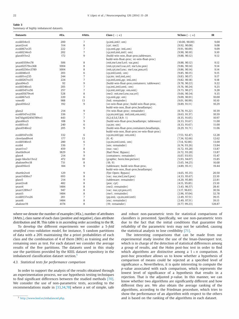
Table 3Summary of highly imbalanced datasets.

Datasets #Ex. #Atts. Class (� ; +) %Class (� ; +) IR

ecoli034vs5 200 7 (p,imL,imU; om) (10.00, 90.00) 9.00yeast2vs4 514 8 (cyt; me2) (9.92, 90.08) 9.08ecoli067vs35 222 7 (cp,omL,pp; imL,om) (9.91, 90.09) 9.09ecoli0234vs5 202 7 (cp,imS,imL,imU; om) (9.90, 90.10) 9.10glass015vs2 172 9 (build-win-non_float-proc,tableware, (9.88, 90.12) 9.12

build-win-float-proc; ve-win-float-proc)yeast0359vs78 506 8 (mit,me1,me3,erl; vac,pox) (9.88, 90.12) 9.12yeast02579vs368 1004 8 (mit,cyt,me3,vac,erl; me1,exc,pox) (9.86, 90.14) 9.14yeast0256vs3789 1004 8 (mit,cyt,me3,exc; me1,vac,pox,erl) (9.86, 90.14) 9.14ecoli046vs5 203 6 (cp,imU,omL; om) (9.85, 90.15) 9.15ecoli01vs235 244 7 (cp,im; imS,imL,om) (9.83, 90.17) 9.17ecoli0267vs35 224 7 (cp,imS,omL,pp; imL,om) (9.82, 90.18) 9.18glass04vs5 92 9 (build-win-float-proc,containers; tableware) (9.78, 90.22) 9.22ecoli0346vs5 205 7 (cp,imL,imU,omL; om) (9.76, 90.24) 9.25ecoli0347vs56 257 7 (cp,imL,imU,pp; om,omL) (9.73, 90.27) 9.28yeast05679vs4 528 8 (me2; mit,me3,exc,vac,erl) (9.66, 90.34) 9.35ecoli067vs5 220 6 (cp,omL,pp; om) (9.09, 90.91) 10.00vowel0 988 13 (hid; remainder) (9.01, 90.99) 10.10glass016vs2 192 9 (ve-win-float-proc; build-win-float-proc, (8.89, 91.11) 10.29

build-win-non_float-proc,headlamps)glass2 214 9 (Ve-win-float-proc; remainder) (8.78, 91.22) 10.39ecoli0147vs2356 336 7 (cp,im,imU,pp; imS,imL,om,omL) (8.63, 91.37) 10.59led7digit02456789vs1 443 7 (0,2,4,5,6,7,8,9; 1) (8.35, 91.65) 10.97glass06vs5 108 9 (build-win-float-proc,headlamps; tableware) (8.33, 91.67) 11.00ecoli01vs5 240 6 (cp,im; om) (8.33, 91.67) 11.00glass0146vs2 205 9 (build-win-float-proc,containers,headlamps, (8.29, 91.71) 11.06

build-win-non_float-proc;ve-win-float-proc)ecoli0147vs56 332 6 (cp,im,imU,pp; om,omL) (7.53, 92.47) 12.28cleveland0vs4 177 13 (0; 4) (7.34, 92.66) 12.62ecoli0146vs5 280 6 (cp,im,imU,omL; om) (7.14, 92.86) 13.00ecoli4 336 7 (om; remainder) (6.74, 93.26) 13.84yeast1vs7 459 8 (nuc; vac) (6.72, 93.28) 13.87shuttle0vs4 1829 9 (Rad Flow; Bypass) (6.72, 93.28) 13.87glass4 214 9 (containers; remainder) (6.07, 93.93) 15.47page-blocks13vs2 472 10 (graphic; horiz.line,picture) (5.93, 94.07) 15.85abalone9vs18 731 8 (18; 9) (5.65, 94.25) 16.68glass016vs5 184 9 (tableware; build-win-float-proc, (4.89, 95.11) 19.44

build-win-non_float-proc,headlamps)shuttle2vs4 129 9 (Fpv Open; Bypass) (4.65, 95.35) 20.50yeast1458vs7 693 8 (vac; nuc,me2,me3,pox) (4.33, 95.67) 22.10glass5 214 9 (tableware; remainder) (4.20, 95.80) 22.81yeast2vs8 482 8 (pox; cyt) (4.15, 95.85) 23.10yeast4 1484 8 (me2; remainder) (3.43, 96.57) 28.41yeast1289vs7 947 8 (vac; nuc,cyt,pox,erl) (3.17, 96.83) 30.56yeast5 1484 8 (me1; remainder) (2.96, 97.04) 32.78ecoli0137vs26 281 7 (pp,imL; cp,im,imU,imS) (2.49, 97.51) 39.15yeast6 1484 8 (exc; remainder) (2.49, 97.51) 39.15abalone19 4174 8 (19; remainder) (0.77, 99.23) 128.87

V. López et al. / Neurocomputing 126 (2014) 15–2822

wherewe denote the number of examples (#Ex.), number of attributes(#Atts.), class name of each class (positive and negative), class attributedistribution and IR. This table is in ascending order according to the IR.

To develop the different experiments we consider a 5-foldstratified cross-validation model, for instance, 5 random partitionsof data with a 20% maintaining the a priori probabilities of eachclass and the combination of 4 of them (80%) as training and theremaining ones as test. For each dataset we consider the averageresults of the five partitions. The datasets used in this studyuse the partitions provided by the KEEL dataset repository in theimbalanced classification dataset section.5

4.3. Statistical tests for performance comparison

In order to support the analysis of the results obtained throughan experimentation process, we use hypothesis testing techniquesto find significant differences between the studied methods [70].We consider the use of non-parametric tests, according to therecommendations made in [33,34,70] where a set of simple, safe

5 http://www.keel.es/imbalanced.php.

and robust non-parametric tests for statistical comparisons ofclassifiers is presented. Specifically, we use non-parametric testsdue to the fact that the initial conditions that guarantee thereliability of the parametric tests may not be satisfied, causingthe statistical analysis to lose credibility [71].

The interesting comparisons that can be made from ourexperimental study involve the use of the Iman-Davenport test,which is in charge of the detection of statistical differences amonga group of results, and the Holm post-hoc test in order to findwhich algorithms are distinctive among a 1�n comparison. Apost-hoc procedure allows us to know whether a hypothesis ofcomparison of means could be rejected at a specified level ofsignificance α. Nevertheless, it is quite interesting to compute thep-value associated with each comparison, which represents thelowest level of significance of a hypothesis that results in arejection. That is the adjusted p-value. In this manner, we canknow whether two algorithms are significantly different and howdifferent they are. We also obtain the average ranking of thealgorithms, according to the Friedman procedure, which tries toshow the performance of an algorithm with respect to the othersand is based on the ranking of the algorithms in each dataset.

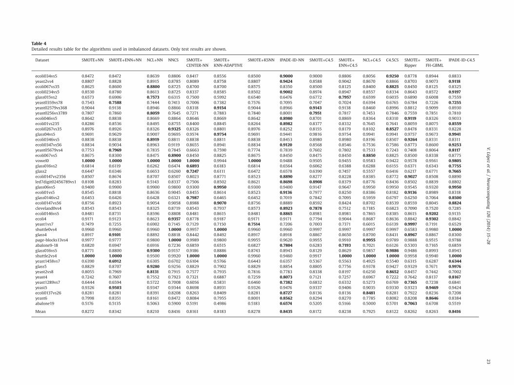
Table 4Detailed results table for the algorithms used in imbalanced datasets. Only test results are shown.

Dataset SMOTE+NN SMOTE+ENN+NN NCL+NN NNCS SMOTE+CENTER-NN

SMOTE+KNN-ADAPTIVE

SMOTE+KSNN IPADE-ID-NN SMOTE+C4.5 SMOTE+ENN+C4.5

NCL+C4.5 C4.5CS SMOTE+Ripper

SMOTE+FH-GBML

IPADE-ID-C4.5

ecoli034vs5 0.8472 0.8472 0.8639 0.8806 0.8417 0.8556 0.8500 0.9000 0.9000 0.8806 0.8056 0.9250 0.8778 0.8944 0.8833yeast2vs4 0.8807 0.8828 0.8915 0.8785 0.8089 0.8758 0.8807 0.9424 0.8588 0.9042 0.8670 0.8866 0.8703 0.9073 0.9118ecoli067vs35 0.8625 0.8600 0.8800 0.8725 0.8700 0.8700 0.8575 0.8350 0.8500 0.8125 0.8400 0.8825 0.8450 0.8125 0.8325ecoli0234vs5 0.8530 0.8780 0.8613 0.8725 0.8337 0.8585 0.8502 0.9002 0.8974 0.8947 0.8557 0.8334 0.8643 0.8572 0.9197glass015vs2 0.6573 0.6906 0.7573 0.6315 0.7500 0.5992 0.6540 0.6476 0.6772 0.7957 0.6599 0.6035 0.6890 0.6008 0.7559yeast0359vs78 0.7543 0.7588 0.7444 0.7413 0.7006 0.7382 0.7576 0.7095 0.7047 0.7024 0.6394 0.6765 0.6784 0.7226 0.7255yeast02579vs368 0.9044 0.9138 0.8946 0.8866 0.8318 0.9154 0.9044 0.8966 0.9143 0.9138 0.8460 0.8996 0.8812 0.9099 0.8930yeast0256vs3789 0.7807 0.7860 0.8059 0.7645 0.7271 0.7883 0.7840 0.8001 0.7951 0.7817 0.7453 0.7846 0.7559 0.7851 0.7810ecoli046vs5 0.8642 0.8838 0.8669 0.8864 0.8646 0.8669 0.8642 0.8980 0.8701 0.8869 0.8364 0.8310 0.9119 0.8326 0.9033ecoli01vs235 0.8286 0.8536 0.8495 0.8755 0.8400 0.8845 0.8264 0.8982 0.8377 0.8332 0.7645 0.7641 0.8059 0.8075 0.8559ecoli0267vs35 0.8976 0.8926 0.8326 0.9325 0.8326 0.8801 0.8976 0.8252 0.8155 0.8179 0.8102 0.8527 0.8478 0.8331 0.8228glass04vs5 0.9691 0.9629 0.9007 0.9695 0.9574 0.9754 0.9691 0.9441 0.9816 0.9754 0.9941 0.9941 0.9757 0.9673 0.9941ecoli0346vs5 0.8838 0.8838 0.8919 0.8811 0.8838 0.8811 0.8838 0.8453 0.8980 0.8980 0.8196 0.8507 0.9264 0.8331 0.8311ecoli0347vs56 0.8834 0.9034 0.8963 0.9119 0.8655 0.8941 0.8834 0.9120 0.8568 0.8546 0.7536 0.7586 0.8773 0.8600 0.9253yeast05679vs4 0.7753 0.7969 0.7835 0.7845 0.6663 0.7590 0.7774 0.7839 0.7602 0.7802 0.7533 0.7243 0.7408 0.8064 0.8117ecoli067vs5 0.8675 0.8300 0.8475 0.8900 0.8450 0.8825 0.8675 0.8450 0.8475 0.8450 0.8850 0.8825 0.8500 0.8338 0.8775vowel0 1.0000 1.0000 1.0000 1.0000 1.0000 0.9944 1.0000 0.9488 0.9505 0.9455 0.9583 0.9422 0.9578 0.9561 0.9805glass016vs2 0.6814 0.6119 0.6262 0.6474 0.6893 0.6183 0.6814 0.6564 0.6062 0.6388 0.6288 0.6155 0.6371 0.6343 0.7755glass2 0.6447 0.6346 0.6653 0.6260 0.7247 0.6111 0.6472 0.6578 0.6390 0.7457 0.5557 0.6416 0.6217 0.6771 0.7665ecoli0147vs2356 0.8507 0.8674 0.8707 0.8507 0.8023 0.8771 0.8523 0.8890 0.8277 0.8228 0.8385 0.8772 0.9027 0.8508 0.8890led7digit02456789vs1 0.8108 0.8283 0.5143 0.8337 0.7506 0.8502 0.8621 0.8698 0.8908 0.8379 0.8776 0.8436 0.8502 0.8839 0.8802glass06vs5 0.9400 0.9900 0.9900 0.9800 0.9300 0.9950 0.9300 0.9400 0.9147 0.9647 0.9950 0.9950 0.9545 0.9320 0.9950ecoli01vs5 0.8545 0.8818 0.8636 0.9045 0.8455 0.8614 0.8523 0.9136 0.7977 0.8250 0.8386 0.8182 0.9136 0.8989 0.8318glass0146vs2 0.6453 0.6426 0.6428 0.6321 0.7987 0.6465 0.6452 0.7019 0.7842 0.7095 0.5959 0.6797 0.6250 0.7064 0.8500ecoli0147vs56 0.8756 0.8923 0.9054 0.9058 0.8988 0.9070 0.8756 0.8889 0.8592 0.8424 0.8702 0.8539 0.8559 0.8045 0.8824cleveland0vs4 0.8543 0.8543 0.8325 0.8719 0.8543 0.7937 0.8573 0.8923 0.7878 0.7512 0.7185 0.6823 0.7090 0.7520 0.7285ecoli0146vs5 0.8481 0.8731 0.8596 0.8808 0.8481 0.8615 0.8481 0.8865 0.8981 0.8981 0.7865 0.8385 0.8615 0.9202 0.9135ecoli4 0.9171 0.9123 0.8623 0.9357 0.8778 0.9187 0.9171 0.9171 0.7794 0.9044 0.8687 0.8636 0.8842 0.9302 0.8842yeast1vs7 0.7479 0.7255 0.6902 0.7145 0.7129 0.7150 0.7514 0.7206 0.7003 0.7371 0.6015 0.6139 0.9997 0.7191 0.6529shuttle0vs4 0.9960 0.9960 0.9960 1.0000 0.9957 1.0000 0.9960 0.9960 0.9997 0.9997 0.9997 0.9997 0.6583 0.9980 1.0000glass4 0.8917 0.9101 0.8892 0.8818 0.8442 0.8492 0.8917 0.8918 0.8867 0.8650 0.8700 0.8431 0.8967 0.8867 0.8300page-blocks13vs4 0.9977 0.9777 0.9800 1.0000 0.9989 0.9800 0.9955 0.9620 0.9955 0.9910 0.9955 0.9789 0.9888 0.9515 0.9788abalone9-18 0.6820 0.6947 0.6916 0.7236 0.6859 0.6515 0.6827 0.7804 0.6283 0.7193 0.7021 0.6126 0.5303 0.7165 0.6859glass016vs5 0.8771 0.8800 0.9300 0.9157 0.9186 0.8886 0.8743 0.8943 0.8129 0.8629 0.9857 0.9886 0.9486 0.8993 0.8943shuttle2vs4 1.0000 1.0000 0.9500 0.9920 1.0000 1.0000 0.9960 0.9460 0.9917 1.0000 1.0000 1.0000 0.9958 0.9940 1.0000yeast1458vs7 0.6390 0.6912 0.6305 0.6702 0.6104 0.5766 0.6443 0.6357 0.5367 0.5563 0.4925 0.5540 0.6315 0.6287 0.6344glass5 0.8829 0.8707 0.9280 0.9256 0.8829 0.7902 0.8829 0.8854 0.8805 0.7756 0.9378 0.9427 0.9329 0.7671 0.9976yeast2vs8 0.8055 0.7969 0.8131 0.7915 0.7577 0.7935 0.7816 0.7783 0.8338 0.8197 0.6250 0.8652 0.8457 0.7442 0.7002yeast4 0.7242 0.7607 0.7552 0.7923 0.7321 0.6887 0.7259 0.8073 0.7121 0.7257 0.6967 0.7222 0.7642 0.8137 0.8167yeast1289vs7 0.6444 0.6594 0.5722 0.7008 0.6056 0.5831 0.6460 0.7382 0.6832 0.6332 0.5273 0.6769 0.7365 0.7238 0.6841yeast5 0.9326 0.9503 0.9347 0.9344 0.8698 0.8931 0.9326 0.9476 0.9337 0.9406 0.9035 0.9330 0.9323 0.9469 0.9424ecoli0137vs26 0.8281 0.8281 0.8391 0.8208 0.8263 0.8409 0.8281 0.8727 0.8136 0.8136 0.8481 0.8281 0.7922 0.8236 0.7208yeast6 0.7998 0.8351 0.8161 0.8472 0.8084 0.7955 0.8001 0.8562 0.8294 0.8270 0.7785 0.8082 0.8208 0.8646 0.8384abalone19 0.5176 0.5135 0.5063 0.5900 0.5191 0.4986 0.5183 0.6574 0.5205 0.5166 0.5000 0.5701 0.7063 0.6708 0.5519

Mean 0.8272 0.8342 0.8210 0.8416 0.8161 0.8183 0.8278 0.8435 0.8172 0.8238 0.7925 0.8122 0.8262 0.8263 0.8416

V.Lópezet

al./Neurocom

puting126

(2014)15

–2823

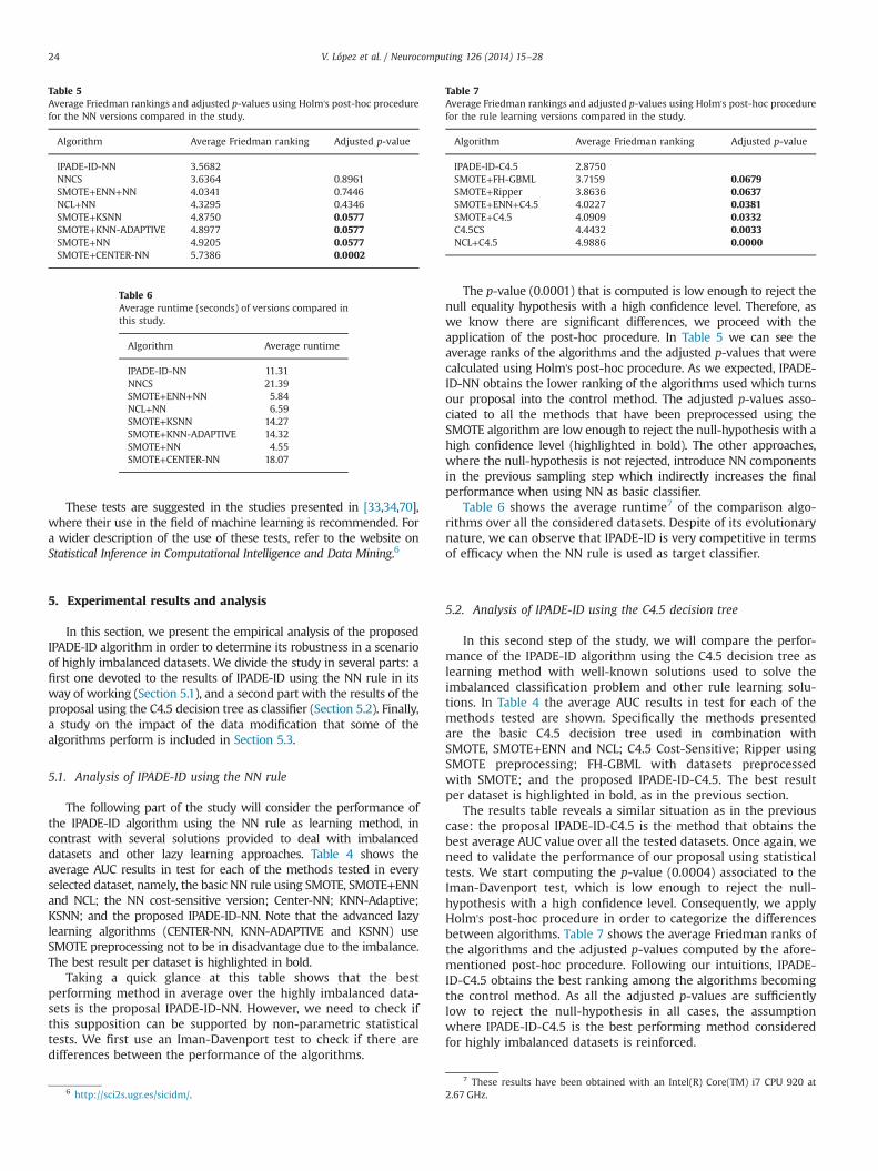
Table 5Average Friedman rankings and adjusted p-values using Holm's post-hoc procedurefor the NN versions compared in the study.

Algorithm Average Friedman ranking Adjusted p-value

IPADE-ID-NN 3.5682NNCS 3.6364 0.8961SMOTE+ENN+NN 4.0341 0.7446NCL+NN 4.3295 0.4346SMOTE+KSNN 4.8750 0.0577SMOTE+KNN-ADAPTIVE 4.8977 0.0577SMOTE+NN 4.9205 0.0577SMOTE+CENTER-NN 5.7386 0.0002

Table 6Average runtime (seconds) of versions compared inthis study.

Algorithm Average runtime

IPADE-ID-NN 11.31NNCS 21.39SMOTE+ENN+NN 5.84NCL+NN 6.59SMOTE+KSNN 14.27SMOTE+KNN-ADAPTIVE 14.32SMOTE+NN 4.55SMOTE+CENTER-NN 18.07

Table 7Average Friedman rankings and adjusted p-values using Holm's post-hoc procedurefor the rule learning versions compared in the study.

Algorithm Average Friedman ranking Adjusted p-value

IPADE-ID-C4.5 2.8750SMOTE+FH-GBML 3.7159 0.0679SMOTE+Ripper 3.8636 0.0637SMOTE+ENN+C4.5 4.0227 0.0381SMOTE+C4.5 4.0909 0.0332C4.5CS 4.4432 0.0033NCL+C4.5 4.9886 0.0000

V. López et al. / Neurocomputing 126 (2014) 15–2824

These tests are suggested in the studies presented in [33,34,70],where their use in the field of machine learning is recommended. Fora wider description of the use of these tests, refer to the website onStatistical Inference in Computational Intelligence and Data Mining.6

5. Experimental results and analysis

In this section, we present the empirical analysis of the proposedIPADE-ID algorithm in order to determine its robustness in a scenarioof highly imbalanced datasets. We divide the study in several parts: afirst one devoted to the results of IPADE-ID using the NN rule in itsway of working (Section 5.1), and a second part with the results of theproposal using the C4.5 decision tree as classifier (Section 5.2). Finally,a study on the impact of the data modification that some of thealgorithms perform is included in Section 5.3.

5.1. Analysis of IPADE-ID using the NN rule

The following part of the study will consider the performance ofthe IPADE-ID algorithm using the NN rule as learning method, incontrast with several solutions provided to deal with imbalanceddatasets and other lazy learning approaches. Table 4 shows theaverage AUC results in test for each of the methods tested in everyselected dataset, namely, the basic NN rule using SMOTE, SMOTE+ENNand NCL; the NN cost-sensitive version; Center-NN; KNN-Adaptive;KSNN; and the proposed IPADE-ID-NN. Note that the advanced lazylearning algorithms (CENTER-NN, KNN-ADAPTIVE and KSNN) useSMOTE preprocessing not to be in disadvantage due to the imbalance.The best result per dataset is highlighted in bold.

Taking a quick glance at this table shows that the bestperforming method in average over the highly imbalanced data-sets is the proposal IPADE-ID-NN. However, we need to check ifthis supposition can be supported by non-parametric statisticaltests. We first use an Iman-Davenport test to check if there aredifferences between the performance of the algorithms.

6 http://sci2s.ugr.es/sicidm/.

The p-value (0.0001) that is computed is low enough to reject thenull equality hypothesis with a high confidence level. Therefore, aswe know there are significant differences, we proceed with theapplication of the post-hoc procedure. In Table 5 we can see theaverage ranks of the algorithms and the adjusted p-values that werecalculated using Holm's post-hoc procedure. As we expected, IPADE-ID-NN obtains the lower ranking of the algorithms used which turnsour proposal into the control method. The adjusted p-values asso-ciated to all the methods that have been preprocessed using theSMOTE algorithm are low enough to reject the null-hypothesis with ahigh confidence level (highlighted in bold). The other approaches,where the null-hypothesis is not rejected, introduce NN componentsin the previous sampling step which indirectly increases the finalperformance when using NN as basic classifier.

Table 6 shows the average runtime7 of the comparison algo-rithms over all the considered datasets. Despite of its evolutionarynature, we can observe that IPADE-ID is very competitive in termsof efficacy when the NN rule is used as target classifier.

5.2. Analysis of IPADE-ID using the C4.5 decision tree

In this second step of the study, we will compare the perfor-mance of the IPADE-ID algorithm using the C4.5 decision tree aslearning method with well-known solutions used to solve theimbalanced classification problem and other rule learning solu-tions. In Table 4 the average AUC results in test for each of themethods tested are shown. Specifically the methods presentedare the basic C4.5 decision tree used in combination withSMOTE, SMOTE+ENN and NCL; C4.5 Cost-Sensitive; Ripper usingSMOTE preprocessing; FH-GBML with datasets preprocessedwith SMOTE; and the proposed IPADE-ID-C4.5. The best resultper dataset is highlighted in bold, as in the previous section.

The results table reveals a similar situation as in the previouscase: the proposal IPADE-ID-C4.5 is the method that obtains thebest average AUC value over all the tested datasets. Once again, weneed to validate the performance of our proposal using statisticaltests. We start computing the p-value (0.0004) associated to theIman-Davenport test, which is low enough to reject the null-hypothesis with a high confidence level. Consequently, we applyHolm's post-hoc procedure in order to categorize the differencesbetween algorithms. Table 7 shows the average Friedman ranks ofthe algorithms and the adjusted p-values computed by the afore-mentioned post-hoc procedure. Following our intuitions, IPADE-ID-C4.5 obtains the best ranking among the algorithms becomingthe control method. As all the adjusted p-values are sufficientlylow to reject the null-hypothesis in all cases, the assumptionwhere IPADE-ID-C4.5 is the best performing method consideredfor highly imbalanced datasets is reinforced.

7 These results have been obtained with an Intel(R) Core(TM) i7 CPU 920 at2.67 GHz.

V. López et al. / Neurocomputing 126 (2014) 15–28 25

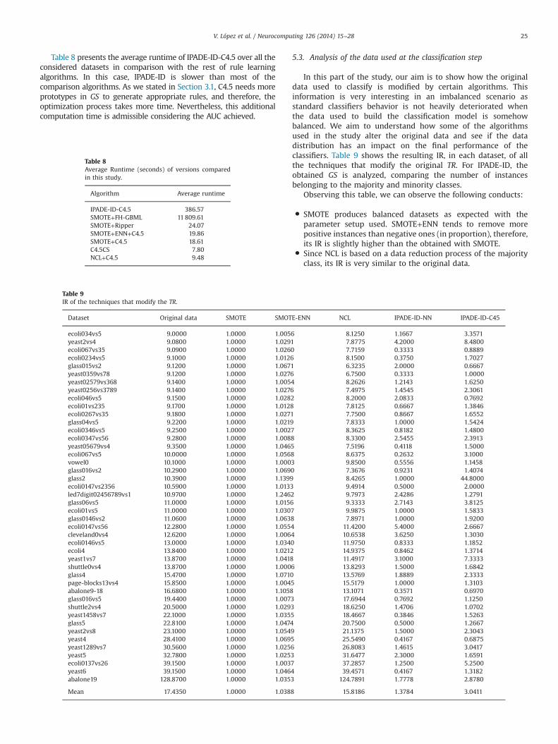
Table 8 presents the average runtime of IPADE-ID-C4.5 over all theconsidered datasets in comparison with the rest of rule learningalgorithms. In this case, IPADE-ID is slower than most of thecomparison algorithms. As we stated in Section 3.1, C4.5 needs moreprototypes in GS to generate appropriate rules, and therefore, theoptimization process takes more time. Nevertheless, this additionalcomputation time is admissible considering the AUC achieved.

Table 9IR of the techniques that modify the TR.

Dataset Original data SMOTE SMOT

ecoli034vs5 9.0000 1.0000 1.005yeast2vs4 9.0800 1.0000 1.029ecoli067vs35 9.0900 1.0000 1.026ecoli0234vs5 9.1000 1.0000 1.012glass015vs2 9.1200 1.0000 1.067yeast0359vs78 9.1200 1.0000 1.027yeast02579vs368 9.1400 1.0000 1.005yeast0256vs3789 9.1400 1.0000 1.027ecoli046vs5 9.1500 1.0000 1.028ecoli01vs235 9.1700 1.0000 1.012ecoli0267vs35 9.1800 1.0000 1.027glass04vs5 9.2200 1.0000 1.021ecoli0346vs5 9.2500 1.0000 1.002ecoli0347vs56 9.2800 1.0000 1.008yeast05679vs4 9.3500 1.0000 1.046ecoli067vs5 10.0000 1.0000 1.056vowel0 10.1000 1.0000 1.000glass016vs2 10.2900 1.0000 1.069glass2 10.3900 1.0000 1.1399ecoli0147vs2356 10.5900 1.0000 1.013led7digit02456789vs1 10.9700 1.0000 1.246glass06vs5 11.0000 1.0000 1.015ecoli01vs5 11.0000 1.0000 1.030glass0146vs2 11.0600 1.0000 1.063ecoli0147vs56 12.2800 1.0000 1.055cleveland0vs4 12.6200 1.0000 1.006ecoli0146vs5 13.0000 1.0000 1.034ecoli4 13.8400 1.0000 1.021yeast1vs7 13.8700 1.0000 1.0418shuttle0vs4 13.8700 1.0000 1.000glass4 15.4700 1.0000 1.071page-blocks13vs4 15.8500 1.0000 1.004abalone9-18 16.6800 1.0000 1.1058glass016vs5 19.4400 1.0000 1.007shuttle2vs4 20.5000 1.0000 1.029yeast1458vs7 22.1000 1.0000 1.035glass5 22.8100 1.0000 1.047yeast2vs8 23.1000 1.0000 1.054yeast4 28.4100 1.0000 1.069yeast1289vs7 30.5600 1.0000 1.025yeast5 32.7800 1.0000 1.025ecoli0137vs26 39.1500 1.0000 1.003yeast6 39.1500 1.0000 1.046abalone19 128.8700 1.0000 1.035

Mean 17.4350 1.0000 1.038

Table 8Average Runtime (seconds) of versions comparedin this study.

Algorithm Average runtime

IPADE-ID-C4.5 386.57SMOTE+FH-GBML 11809.61SMOTE+Ripper 24.07SMOTE+ENN+C4.5 19.86SMOTE+C4.5 18.61C4.5CS 7.80NCL+C4.5 9.48

5.3. Analysis of the data used at the classification step

In this part of the study, our aim is to show how the originaldata used to classify is modified by certain algorithms. Thisinformation is very interesting in an imbalanced scenario asstandard classifiers behavior is not heavily deteriorated whenthe data used to build the classification model is somehowbalanced. We aim to understand how some of the algorithmsused in the study alter the original data and see if the datadistribution has an impact on the final performance of theclassifiers. Table 9 shows the resulting IR, in each dataset, of allthe techniques that modify the original TR. For IPADE-ID, theobtained GS is analyzed, comparing the number of instancesbelonging to the majority and minority classes.

Observing this table, we can observe the following conducts:

�

E-E

610616462819785830

326784402

605

33549563743

8

SMOTE produces balanced datasets as expected with theparameter setup used. SMOTE+ENN tends to remove morepositive instances than negative ones (in proportion), therefore,its IR is slightly higher than the obtained with SMOTE.

�

Since NCL is based on a data reduction process of the majorityclass, its IR is very similar to the original data.

NN NCL IPADE-ID-NN IPADE-ID-C45

8.1250 1.1667 3.35717.8775 4.2000 8.48007.7159 0.3333 0.88898.1500 0.3750 1.70276.3235 2.0000 0.66676.7500 0.3333 1.00008.2626 1.2143 1.62507.4975 1.4545 2.30618.2000 2.0833 0.76927.8125 0.6667 1.38467.7500 0.8667 1.65527.8333 1.0000 1.54248.3625 0.8182 1.48008.3300 2.5455 2.39137.5196 0.4118 1.50008.6375 0.2632 3.10009.8500 0.5556 1.14587.3676 0.9231 1.40748.4265 1.0000 44.80009.4914 0.5000 2.00009.7973 2.4286 1.27919.3333 2.7143 3.81259.9875 1.0000 1.58337.8971 1.0000 1.920011.4200 5.4000 2.666710.6538 3.6250 1.303011.9750 0.8333 1.185214.9375 0.8462 1.371411.4917 3.1000 7.333313.8293 1.5000 1.684213.5769 1.8889 2.333315.5179 1.0000 1.310313.1071 0.3571 0.697017.6944 0.7692 1.125018.6250 1.4706 1.070218.4667 0.3846 1.526320.7500 0.5000 1.266721.1375 1.5000 2.304325.5490 0.4167 0.687526.8083 1.4615 3.041731.6477 2.3000 1.659137.2857 1.2500 5.250039.4571 0.4167 1.3182

124.7891 1.7778 2.8780

15.8186 1.3784 3.0411

V. López et al. / Neurocomputing 126 (2014) 15–2826

�

In general, the IPADE-ID scheme does not need to balanceclasses to obtain good generalization results. The generateddataset is very dependent of the problem tackled and the usedclassifier, so that the corresponding IR is not related to theoriginal IR. It is noteworthy that in many problems, the IPADE-ID algorithm generates more positives instances with respect tothe negative ones because it is the most complex class.

�

The main difference between IPADE-ID-NN and IPADE-ID-C4.5is that the NN version is more balanced. It means that C4.5needs more instances in the negative class to represent itsdecision boundaries.

To sum up, our experimental study has shown that IPADE-ID isan algorithm that presents a good performance in the scenario ofhighly imbalanced datasets. The integration of instance generationtechniques in a resampling step produces an improvement ofthe results in this unfavorable scenario. Furthermore, the methodhas shown its robustness with two different learning paradigms,taking into consideration the features of the learning methods intothe way of working of the proposal.

6. Concluding remarks

In this paper, we have presented IPADE-ID, a new approach todeal with the problem of classification with highly imbalanceddatasets. The proposal provides a solution that modifies thetraining set using a IG technique based on differential evolutionas base for the procedure, adapting its way of working to thisimbalanced scenario. As learning methods, we have selected theNN rule and the C4.5 decision tree and we have adapted theIPADE-ID approach according to these methods behavior.

The experimental study performed has shown that the usage ofinstance generation techniques to deal with highly imbalanceddatasets can be taken into consideration as a valid solution to thisproblem. IPADE-ID has demonstrated its good behavior in anexhaustive comparison with methodologies that are used to solvethis problem such as resampling techniques or cost-sensitivesolutions. The proposal outperforms the other approaches in thescenario of highly imbalanced datasets, which usually is a scenariowhere most algorithms have lots of difficulties to perform prop-erly. On the other hand, the proposal obtains a good performanceusing different techniques as learning methods, which makes itextensible to other learning paradigms and permits a furtheradaptation of the presented proposal into more powerful solutionsthat adapt the procedure at the algorithm level.

Acknowledgments

This work was partially supported by the Spanish Ministry ofScience and Technology under project TIN2011-28488 and theAndalusian Research Plans P11-TIC-7765 and P10-TIC-6858. V. Lópezholds a FPU scholarship from Spanish Ministry of Education.

References

[1] Y. Sun, A.K.C. Wong, M.S. Kamel, Classification of imbalanced data: a review,International Journal of Pattern Recognition and Artificial Intelligence 23 (4)(2009) 687–719.

[2] H. He, E.A. Garcia, Learning from imbalanced data, IEEE Transactions onKnowledge and Data Engineering 21 (9) (2009) 1263–1284.

[3] C. Elkan, The foundations of cost-sensitive learning, in: Proceedings of the17th IEEE International Joint Conference on Artificial Intelligence (IJCAI'01),2001, pp. 973–978.

[4] B. Zadrozny, J. Langford, N. Abe, Cost-sensitive learning by cost-proportionateexample weighting, in: Proceedings of the 3rd IEEE International Conferenceon Data Mining (ICDM'03), 2003, pp. 435–442.

[5] G.M. Weiss, Mining with rarity: a unifying framework, SIGKDD Explorations6 (1) (2004) 7–19.

[6] N. Japkowicz, S. Stephen, The class imbalance problem: a systematic study,Intelligent Data Analysis Journal 6 (5) (2002) 429–450.

[7] V. López, A. Fernández, J.G. Moreno-Torres, F. Herrera, Analysis of preproces-sing vs. cost-sensitive learning for imbalanced classification. Open problemson intrinsic data characteristics, Expert Systems with Applications 39 (7)(2012) 6585–6608.

[8] T. Yu, S. Simoff, T. Jan, VQSVM: a case study for incorporating prior domainknowledge into inductive machine learning, Neurocomputing 73 (13–15)(2010) 2614–2623.

[9] S.-H. Oh, Error back-propagation algorithm for classification of imbalanceddata, Neurocomputing 74 (6) (2011) 1058–1061.

[10] N.V. Chawla, K.W. Bowyer, L.O. Hall, W.P. Kegelmeyer, SMOTE: syntheticminority over-sampling technique, Journal of Artificial Intelligent Research16 (2002) 321–357.

[11] G.E.A.P.A. Batista, R.C. Prati, M.C. Monard, A study of the behaviour of severalmethods for balancing machine learning training data, SIGKDD Explorations6 (1) (2004) 20–29.

[12] S. García, J. Derrac, I. Triguero, C.J. Carmona, F. Herrera, Evolutionary-basedselection of generalized instances for imbalanced classification, Knowledge-Based Systems 25 (1) (2012) 3–12.

[13] D.R. Wilson, T.R. Martinez, Reduction techniques for instance-based learningalgorithms, Machine Learning 38 (3) (2000) 257–286.

[14] I. Kononenko, M. Kukar, Machine Learning and Data Mining: Introduction toPrinciples and Algorithms, Horwood Publishing Limited, 2007.

[15] S. García, A. Fernández, F. Herrera, Enhancing the effectiveness and interpret-ability of decision tree and rule induction classifiers with evolutionary trainingset selection over imbalanced problems, Applied Soft Computing 9 (2009)1304–1314.

[16] A. de Haro-Garcia, N. Garcia-Pedrajas, A scalable method for instance selection forclass-imbalance datasets, in: Proceedings of the 11th International Conference onIntelligent Systems Design and Applications (ISDA'11), 2011, pp. 1383–1390.

[17] J. Derrac, S. García, F. Herrera, IFS-CoCo: instance and feature selection basedon cooperative coevolution with nearest neighbor rule, Pattern Recognition43 (6) (2010) 2082–2105.

[18] S. García, J. Derrac, J. Cano, F. Herrera, Prototype selection for nearest neighborclassification: taxonomy and empirical study, IEEE Transactions on PatternAnalysis and Machine Intelligence 34 (3) (2012) 417–435.

[19] H.A. Fayed, S.R. Hashem, A.F. Atiya, Self-generating prototypes for patternclassification, Pattern Recognition 40 (5) (2007) 1498–1509.

[20] I. Triguero, J. Derrac, S. García, F. Herrera, A taxonomy and experimental studyon prototype generation for nearest neighbor classification, IEEE Transactionson Systems, Man, and Cybernetics-Part C: Applications and Reviews 42 (1)(2012) 86–100.

[21] S. García, F. Herrera, Evolutionary under-sampling for classification withimbalanced data sets: proposals and taxonomy, Evolutionary Computation17 (3) (2009) 275–306.

[22] I. Triguero, S. García, F. Herrera, IPADE: iterative prototype adjustment fornearest neighbor classification, IEEE Transactions on Neural Networks 21 (12)(2010) 1984–1990.

[23] I. Triguero, S. García, F. Herrera, Enhancing IPADE algorithm with adifferent individual codification, in: Proceedings of the Sixth InternationalConference on Hybrid Artificial Intelligence Systems (HAIS'11), 2011, pp. 262–270.

[24] T.M. Cover, P.E. Hart, Nearest neighbor pattern classification, IEEE Transactionson Information Theory 13 (1) (1967) 21–27.

[25] J.R. Quinlan, C4.5: Programs for Machine Learning, Morgan Kaufmann Publish-ers, San Francisco, CA, USA, 1993.

[26] R. Storn, K.V. Price, Differential evolution – a simple and efficient heuristic forglobal optimization over continuous spaces, Journal of Global Optimization 11(10) (1997) 341–359.

[27] K.V. Price, R.M. Storn, J.A. Lampinen, Differential evolution: a practicalapproach to global optimization, Natural Computing Series (2005).

[28] F. Neri, V. Tirronen, Scale factor local search in differential evolution, MemeticComputing 1 (2) (2009) 153–171.

[29] E. Corchado, A. Abraham, A. Carvalho, Hybrid intelligent algorithms andapplications, Information Sciences 180 (14) (2010) 2633–2634.

[30] E. Corchado, M. Graña, M. Wozniak, New trends and applications on hybridartificial intelligence systems, Neurocomputing 75 (1) (2012) 61–63.

[31] J. Alcalá-Fdez, A. Fernandez, J. Luengo, J. Derrac, S. García, L. Sánchez,F. Herrera, KEEL data-mining software tool: data set repository, integrationof algorithms and experimental analysis framework, Journal of Multiple-Valued Logic and Soft Computing 17 (2–3) (2011) 255–287.

[32] J. Huang, C.X. Ling, Using AUC and accuracy in evaluating learning algorithmsIEEE Transactions on Knowledge and Data Engineering 17 (3) (2005) 299–310.

[33] J. Demšar, Statistical comparisons of classifiers over multiple data sets, Journalof Machine Learning Research 7 (2006) 1–30.

[34] S. García, F. Herrera, An extension on “statistical comparisons of classifiersover multiple data sets” for all pairwise comparisons, Journal of MachineLearning Research 9 (2008) 2677–2694.

[35] L. Nanni, A. Lumini, Particle swarm optimization for prototype reduction,Neurocomputing 72 (4–6) (2008) 1092–1097.

[36] J.S. Sánchez, R. Barandela, A.I. Marqués, R. Alejo, J. Badenas, Analysis of newtechniques to obtain quality training sets, Pattern Recognition Letters 24 (7)(2003) 1015–1022.

[37] J.S. Sánchez, High training set size reduction by space partitioning andprototype abstraction, Pattern Recognition 37 (7) (2004) 1561–1564.

V. López et al. / Neurocomputing 126 (2014) 15–28 27

[38] I. Triguero, S. García, F. Herrera, Differential evolution for optimizing thepositioning of prototypes in nearest neighbor classification, Pattern Recogni-tion 44 (4) (2011) 901–916.

[39] T. Kohonen, The self organizing map, Proceedings of the IEEE 78 (9) (1990)1464–1480.

[40] W.-J. Lin, J. Chen, Biomarker classifiers for identifying susceptible subpopula-tions for treatment decisions, Pharmacogenomics 13 (2) (2012) 147–157.

[41] I. Brown, C. Mues, An experimental comparison of classification algorithms forimbalanced credit scoring data sets, Expert Systems with Applications 39 (3)(2012) 3446–3453.

[42] J. Xiao, L. Xie, C. He, X. Jiang, Dynamic classifier ensemble model for customerclassification with imbalanced class distribution, Expert Systems with Appli-cations 39 (3) (2012) 3668–3675.

[43] W. Khreich, E. Granger, A. Miri, R. Sabourin, Iterative boolean combination ofclassifiers in the ROC space: an application to anomaly detection with HMMs,Pattern Recognition 43 (8) (2010) 2732–2752.

[44] N. García-Pedrajas, J. Pérez-Rodríguez, M. García-Pedrajas, D. Ortiz-Boyer,C. Fyfe, Class imbalance methods for translation initiation site recognition indna sequences, Knowledge-Based Systems 25 (1) (2012) 22–34.

[45] A. Orriols-Puig, E. Bernadó-Mansilla, Evolutionary rule-based systems forimbalanced datasets, Soft Computing 13 (3) (2009) 213–225.

[46] V. García, R. Mollineda, J.S. Sánchez, On the k-NN performance in a challengingscenario of imbalance and overlapping, Pattern Analysis Applications 11 (3–4)(2008) 269–280.

[47] G.M. Weiss, F. Provost, Learning when training data are costly: the effect ofclass distribution on tree induction, Journal of Artificial Intelligence Research19 (2003) 315–354.

[48] R.C. Prati, G.E.A.P.A. Batista, M.C. Monard, Learning with class skews and smalldisjuncts, in: Seventeenth Brazilian Symposium on Artificial Intelligence(SBIA2004), 2004, pp. 296–306.

[49] J.G. Moreno-Torres, T. Raeder, R. Alaíz-Rodríguez, N.V. Chawla, F. Herrera, Aunifying view on dataset shift in classification, Pattern Recognition 45 (1)(2012) 521–530.

[50] K. Napierala, J. Stefanowski, S. Wilk, Learning from imbalanced data inpresence of noisy and borderline examples, in: Seventh International Con-ference on Rough Sets and Current Trends in Computing (RSCTC2010), 2010,pp. 158–167.

[51] J. Laurikkala, Improving identification of difficult small classes by balancingclass distribution, in: Proceedings of the Eighth Conference on AI in Medicinein Europe (AIME'01), 2001, pp. 63–66.

[52] D.L. Wilson, Asymptotic properties of nearest neighbor rules using edited data,IEEE Transactions on System, Man and Cybernetics 2 (3) (1972) 408–421.

[53] H. Han, W. Wang, B. Mao, Borderline-SMOTE: a new over-sampling method inimbalanced data sets learning, in: Proceedings of the 2005 InternationalConference on Intelligent Computing (ICIC'05), Lecture Notes in ComputerScience, vol. 3644, 2005, pp. 878–887.

[54] H. He, Y. Bai, E. Garcia, S. Li, ADASYN: adaptive synthetic sampling approachfor imbalanced learning, in: Proceedings of the 2008 IEEE International JointConference Neural Networks (IJCNN'08), 2008, pp. 1322–1328.

[55] C. Bunkhumpornpat, K. Sinapiromsaran, C. Lursinsap, Safe-level-SMOTE: safe-level-synthetic minority over-sampling Technique for handling the class imbal-anced problem, in: Proceedings of the 13th Pacific-Asia Conference on Advances inKnowledge Discovery and Data Mining PAKDD'09, 2009, pp. 475–482.

[56] T.M. Khoshgoftaar, N. Seliya, D.J. Drown, Evolutionary data analysis for theclass imbalance problem, Intelligent Data Analysis 14 (1) (2010) 69–88.

[57] W. Cohen, Fast effective rule induction, in: Proceedings of the 12th Interna-tional Conference on Machine Learning (ICML'95), 1995, pp. 1–10.

[58] J. Luengo, A. Fernández, S. García, F. Herrera, Addressing data complexity forimbalanced data sets: analysis of SMOTE-based oversampling and evolution-ary undersampling, Soft Computing 15 (10) (2011) 1909–1936.

[59] E. Frank, I. Witten, Generating accurate rule sets without global optimization,in: Proceedings of the Fifteenth International Conference on Machine Learn-ing, 1998, pp. 144–151.

[60] S. Salzberg, A nearest hyperrectangle learning method, Machine Learning 6(1991) 251–276.

[61] A.P. Bradley, The use of the area under the ROC curve in the evaluation ofmachine learning algorithms, Pattern Recognition 30 (7) (1997) 1145–1159.

[62] M. Lozano, J.M. Sotoca, J.S. Sánchez, F. Pla, E. Pekalska, R.P.W. Duin, Experi-mental study on prototype optimisation algorithms for prototype-basedclassification in vector spaces, Pattern Recognition 39 (10) (2006) 1827–1838.

[63] R. Barandela, J.S. Sánchez, V. García, E. Rangel, Strategies for learning in classimbalance problems, Pattern Recognition 36 (3) (2003) 849–851.

[64] K.M. Ting, An instance-weighting method to induce cost-sensitive trees, IEEETransactions on Knowledge and Data Engineering 14 (3) (2002) 659–665.

[65] Q. Gao, Z. Wang, Center-based nearest neighbor classifier, Pattern Recognition40 (2007) 346–349.

[66] J. Wang, P. Neskovic, L. Cooper, Improving nearest neighbor rule with a simpleadaptative distance measure, Pattern Recognition Letters 28 (2007) 207–213.

[67] R. Nock, M. Sebban, D. Bernard, A simple locally adaptive nearest neighborrule with application to pollution forecasting, International Journal of PatternRecognition and Artificial Intelligence 17 (2003) 1369–1382.

[68] H. Ishibuchi, T. Yamamoto, T. Nakashima, Hybridization of fuzzy GBMLapproaches for pattern classification problems, IEEE Transactions on Systemsand Man and Cybernetics-Part B: Cybernetics 35 (2) (2005) 359–365.

[69] J. Alcalá-Fdez, L. Sánchez, S. García, M.J. del Jesus, S. Ventura, J.M. Garrell,J. Otero, C. Romero, J. Bacardit, V.M. Rivas, J.C. Fernández, F. Herrera, KEEL: a

software tool to assess evolutionary algorithms for data mining problems, SoftComputing 13 (3) (2009) 307–318.

[70] S. García, A. Fernández, J. Luengo, F. Herrera, A study of statistical techniquesand performance measures for genetics-based machine learning: accuracyand interpretability, Soft Computing 13 (10) (2009) 959–977.

[71] D.J. Sheskin, Handbook of Parametric and Nonparametric Statistical Proce-dures, 5th ed., Chapman & Hall/CRC, 2011.

Victoria López received her M.Sc. degree in ComputerScience from the University of Granada, Granada, Spain, in2009. She is currently a Ph.D. student in the Departmentof Computer Science and Artificial Intelligence, Universityof Granada, Granada, Spain. Her research interests includedata mining, classification in imbalanced domains, fuzzyrule learning and evolutionary algorithms.

Isaac Triguero received the M.Sc. degree in ComputerScience from the University of Granada, Granada, Spain,in 2009. He is currently a Ph.D. student in the Depart-ment of Computer Science and Artificial Intelligence,University of Granada, Granada, Spain. His researchinterests include data mining, semisupervised learning,data reduction and evolutionary algorithms.

Cristóbal José Carmona received the M.Sc. and Ph.D.degrees in computer science from the University ofJaén, Spain, in 2006 and 2011, respectively. He is aresearcher in the Department of Computer Science,University of Jaén, Spain. Currently, he is working withIntelligent Systems and Data Mining Research Group ofJaén. His research interest includes supervised descrip-tive rule discovery, subgroup discovery, contrast setmining, emerging pattern mining, evolutionary fuzzysystems, evolutionary algorithm and data mining.

Salvador García received the M.Sc. and Ph.D. degrees inComputer Science from the University of Granada,Granada, Spain, in 2004 and 2008, respectively. He iscurrently an Associate Professor in the Department ofComputer Science, University of Jaén, Jaén, Spain. Hehas had more than 25 papers published in internationaljournals. He has co-edited two special issues ofinternational journals on different Data Mining topics.His research interests include data mining, data reduc-tion, data complexity, imbalanced learning, semi-supervised learning, statistical inference and evolution-ary algorithms.

Francisco Herrera received his M.Sc. in Mathematics in1988 and Ph.D. in Mathematics in 1991, both from theUniversity of Granada, Spain.

He is currently a Professor in the Department ofComputer Science and Artificial Intelligence at theUniversity of Granada. He has had more than 200papers published in international journals. He is coau-thor of the book “Genetic Fuzzy Systems: EvolutionaryTuning and Learning of Fuzzy Knowledge Bases” (WorldScientific, 2001).

He currently acts as Editor in Chief of the internationaljournal “Progress in Artificial Intelligence (Springer) and

serves as area editor of the Journal Soft Computing (area of

evolutionary and bioinspired algorithms) and International Journal of ComputationalIntelligence Systems (area of information systems). He acts as associated editor of the

V. López et al. / Neurocomputing 126 (2014) 15–2828

journals: IEEE Transactions on Fuzzy Systems, Information Sciences, Advances in FuzzySystems, and International Journal of Applied Metaheuristics Computing; and he servesas member of several journal editorial boards, among others: Fuzzy Sets and Systems,Applied Intelligence, Knowledge and Information Systems, Information Fusion, Evolu-tionary Intelligence, International Journal of Hybrid Intelligent Systems, MemeticComputation, Swarm and Evolutionary Computation.

He received the following honors and awards: ECCAI Fellow 2009, 2010 SpanishNational Award on Computer Science ARITMEL to the “Spanish Engineer on Computer

Science”, and International Cajastur “Mamdani” Prize for Soft Computing (FourthEdition, 2010).

His current research interests include computing with words and decision making,data mining, bibliometrics, data preparation, instance selection, fuzzy rule basedsystems, genetic fuzzy systems, knowledge extraction based on evolutionary algorithms,memetic algorithms and genetic algorithms.