LASzip: lossless compression of LiDAR dataMartin Isenburg

LAStoolshttp://laszip.org

Abstract—Airborne laser scanning technology (LiDAR) makesit easy to collect large amounts of point data that sample theelevation of the terrain beneath. The LAS format has become thede facto standard for storing and distributing the acquired points.As the sampling density of LiDAR increases so does the size ofthe resulting files. Typical LAS files contain tens to hundreds ofmillions points today, but soon billions will be commonplace.

We describe a completely lossless compression scheme forLiDAR in binary LAS format versions 1.0 to 1.3. Our encodingand decoding speeds are around one to three millions points persecond and our compressed files are only 7 to 25 percent of theoriginal file size. Compression and decompression happen on-the-fly in a streaming manner and random-access is supported with adefault granularity of 50,000 points. A reference implementationunencumbered by patents or intellectual property concerns isfreely available with an LGPL-license, making the proposedcompression scheme suitable to become part of the LAS standard.

I. INTRODUCTION

Low flying aircrafts equipped with modern laser-range scan-ning technology (LiDAR) collect precise elevation informationfor entire cities, counties, or even states. Shooting 100,000 ormore laser pulses per second onto the earth’s surface theytake measurements at resolutions exceeding one point persquare meter. Derivatives of this data such as digital elevationmaps are subsequently used in numerous applications: toassess flood hazards, plan solar and wind installations, carryout forest inventories, aid in power grid maintenance, etc.However, the sheer amount of LiDAR data collected posesa significant challenge as not millions but billions of elevationsamples need to be stored, processed, and distributed.

The scanner records the waveform of the returning reflectionfor each laser pulse that it sends out. The intensity peaks ofthis waveform correspond to points that were hit by the laserand that reflected significant portions back to the sensors onthe plane. There can be multiple peaks because the laser mayhit several surfaces such as wires or antennas, branches, leaves,or even birds in flight before reaching the ground. Each peakabove a certain threshold is called a return. The coordinatesof these returns together with intensity, scan angle, GPS time,return number, flight line ID, etc. are the data of interest.

Fresh off the scanner, the LiDAR data is typically storedin a binary, vendor-specific format. But to exchange the databetween users and across different software packages it wastraditionally converted into a simple ASCII representationwhere each line was listing the attributes of a single return.While flexible and easy to understand, storing millions (or nowbillions) of LiDAR returns in a textual format is cumbersome:the file size grows large, parsing the data is inefficient, and it is

not possible to seek within the file. Addressing these concernsthe ASPRS created a simple binary exchange format - the LASformat [1]. It is now the de facto industry standard for storageand distribution of airborne and mobile LiDAR data.

Up to LAS 1.3, each point record has a core 20 bytes ofwhich 12 bytes store the x, y, and z coordinate as signedintegers. The header of a LAS file contains scaling factorsfor those integers that specify the precision (e.g. such as0.01 for cm and 0.001 for mm). The other 8 bytes storeintensity, scan angle, return count, classifications, etc. Thiscompletes the basic point type 0 (for details see Table I). Thepoint types 1 and 3 add an 8 byte GPS time and the pointtypes 2 and 3 provide 6 bytes to store an RGB color. TheLAS 1.3 specification introduced the point types 4 and 5 thatallow attaching full waveform information to each return (withcontroversial design choices) but they are not used much.

One of the great features of the LAS format is that it storesthe coordinates as scaled and offset integers—thereby requir-ing the producers to think about the actual precision in theirscanned data samples and to choose appropriate incrementssuch as 0.01 meters (or feet) for storing the coordinates. Thiseliminates the unnecessary if not disastrous bloat of double-precision floats or 20 digit ASCII representations where 15of the 20 digits are really just scanner noise. The absence ofincompressible noise makes it possible to efficiently compressthe LiDAR points in a completely lossless manner.

Generic compression schemes are not well suited to com-press LiDAR because they do not have the insights into thestructure of the data to properly model the probabilities ofcertain patterns to occur. The WinZIP compressor does notcompress well while the WinRAR compressor is extremelyslow. Neither scheme is suited for streaming or for random-access decompression, which means the entire file needs to bedecompressed before its contents can be accessed.

In this paper we introduce LASzip, a lossless compressor forLiDAR stored in the LAS format. It delivers high compressionrates at unmatched speeds and supports streaming, random-access decompression. The source code is available withLGPL-license and was integrated into the open source librariesLASlib of LAStools [2] and libLAS [3]. There is nativesupport for reading and writing LAZ in FME 2012, TopoDOT,VoyagerGIS, and LAStools and others are following. LAZ isused internally at USACE, Certainty3D, Watershed Sciences,Riegl, and others. Data providers such as Open Topographyprovide LAZ as an compressed download option [4] and theDNR of Minnesota hosts LiDAR for 40 counties exclusivelyin LAZ format with plans to complete the entire state [5].

II. BACKGROUND

Before describing the LASzip compressor some preliminar-ies about coordinate precision, the LAS format, related workin point compression, and entropy and difference coding.

A. Floating-Point Precision vs. Integer Precision

There is a common miss-conception that floating-point rep-resentations provide more precision than integer presentationsfor storing the x, y, z coordinates of a point. They do not.

The coordinates of LiDAR points from an airborne or amobile survey are spread out in the x-y plane with uniformdistribution, in the sense that there are roughly the samenumber of points per square meter everywhere and that thepoints are acquired with roughly the same precision. Therewill not be one particularly dense area where points need tobe stored with higher precision. The floating-point format isnot designed for storing uniform distributions of numbers.

Storing a number in floating-point representation means thatthe precision of the number will vary depending on the value ofthat number. The closer it gets to zero the more precision it willhave. This makes it a good format, for example, for numericalcomputations where more precision is needed closer to zero.But using the floating-point format to store point coordinatesmeans that there is an increasingly precise spacing of datasamples around one point—the origin—at the expense of anincreasingly imprecise spacing farther away.

An example: in single-precision floating-point there are 223

different numbers to represent a coordinate between 2 and4 meters with a spacing of 2/223 = 0.00000023841 meter,there are 223 different numbers to represent a coordinatebetween 128 and 256 meters with a spacing of 128/223 =0.00001525 meter, there are 223 different numbers to representa coordinate between 524, 288 and 1, 048, 576 meters witha spacing of 524, 288/223 = 0.0625 meter, and of coursethere are also 223 different numbers to represent a coordinatebetween 2, 097, 152 and 4, 194, 304 meters with a spacing of4, 194, 304/223 = 0.25 meter. If you notice the pattern youalready know that there will also be 223 different numbersto represent a coordinate between 4, 194, 304 and 8, 388, 608meters with a spacing of 4, 194, 304/223 = 0.5 meter.

In summary, if you store the easting and northing of yourcoordinates directly in floating-point they may retain just 0.5meters of precision. If you subtract a constant offset from yourcoordinates so the origin falls into the middle of the boundingbox, then the samples near the origin are stored with incredibleprecision ... much much more than LiDAR has.

The appropriate format for storing the coordinates of LiDARpoints are properly scaled and offset integers. They offermuch more uniform precision than a corresponding floating-point value for the same number of bits: a 32 bit integer,for example, offers 7 bits more uniform precision than a 32bit floating-point number [6] and similarly a 64 bit integeroffers 10 bits more than a 64 bit float. In order to increase thecoordinate range for a large-scale LiDAR collect, the correctthing to do is to move from 32 bit to 64 bit integers. The LASformat [1] uses scaled and offset 32 bit integers.

name of atomic item size point type and size0 1 2 3 4 5

point attributes format size 20 28 26 34 57 63

POINT10 20 bytes x x x x x xX int 4 bytes x x x x x xY int 4 bytes x x x x x xZ int 4 bytes x x x x x xIntensity u short 2 bytes x x x x x xReturn Number 3 bits 3 bits x x x x x xNumber of Returns of Pulse 3 bits 3 bits x x x x x xScan Direction Flag 1 bit 1 bit x x x x x xEdge of Flight Line 1 bit 1 bit x x x x x xClassification u char 1 byte x x x x x xScan Angle Rank u char 1 byte x x x x x xUser Data u char 1 byte x x x x x xPoint Source ID u short 2 bytes x x x x x x

GPSTIME10 8 bytes x x x xGPS Time double 8 bytes x x x x

RGB12 6 bytes x x xRed u short 2 bytes x x xGreen u short 2 bytes x x xBlue u short 2 bytes x x x

WAVEPACKET13 29 bytes x xWave Packet Descriptor Index u char 1 byte x xBytes Offset to Waveform Data u int64 8 bytes x xWaveform Packet Size in Bytes u int 4 bytes x xReturn Point Waveform Location float 4 bytes x xX(t) float 4 bytes x xY(t) float 4 bytes x xZ(t) float 4 bytes x x

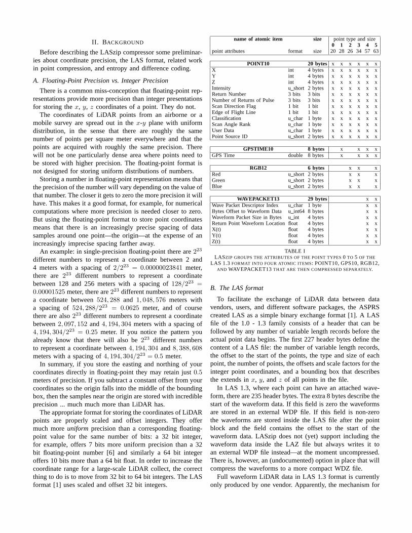
TABLE ILASZIP GROUPS THE ATTRIBUTES OF THE POINT TYPES 0 TO 5 OF THE

LAS 1.3 FORMAT INTO FOUR ATOMIC ITEMS: POINT10, GPS10, RGB12,AND WAVEPACKET13 THAT ARE THEN COMPRESSED SEPARATELY.

B. The LAS format

To facilitate the exchange of LiDAR data between datavendors, users, and different software packages, the ASPRScreated LAS as a simple binary exchange format [1]. A LASfile of the 1.0 - 1.3 family consists of a header that can befollowed by any number of variable length records before theactual point data begins. The first 227 header bytes define thecontent of a LAS file: the number of variable length records,the offset to the start of the points, the type and size of eachpoint, the number of points, the offsets and scale factors for theinteger point coordinates, and a bounding box that describesthe extends in x, y, and z of all points in the file.

In LAS 1.3, where each point can have an attached wave-form, there are 235 header bytes. The extra 8 bytes describe thestart of the waveform data. If this field is zero the waveformsare stored in an external WDP file. If this field is non-zerothe waveforms are stored inside the LAS file after the pointblock and the field contains the offset to the start of thewaveform data. LASzip does not (yet) support including thewaveform data inside the LAZ file but always writes it toan external WDP file instead—at the moment uncompressed.There is, however, an (undocumented) option in place that willcompress the waveforms to a more compact WDZ file.

Full waveform LiDAR data in LAS 1.3 format is currentlyonly produced by one vendor. Apparently, the mechanism for

waveform storage was quickly added to the LAS standardto meet the needs of one hardware vendor without seekingmutual consensus among all scanner manufacturers first. Thereis almost no publicly available waveform data stored in theLAS 1.3 format and there are only a few software products thatcan make use of the waveform data in LAS 1.3 files. Thereforewe postpone the details for full waveform compression forLAS 1.3 until it becomes more relevant.

The point types 0 to 5 available in LAS 1.3 and theattributes they are composed of are detailed in Table I. TheLASzip compressor views point types as compositions offour different atomic items: POINT10, GPSTIME10, RGB12,and WAVEPACKET13 that are compressed separately. Forexample, a point of type 3 is composed of POINT10 followedby GPSTIME10 and RGB12. Additionally each point mayhave n so called “extra bytes” at the end, each of which iscurrently considered as a BYTE item. These “extra bytes”occur when the LAS header specifies a point size larger thanrequired by the respective point type. For example if the pointtype is 1 and the point size is 32 then there are 4 “extra bytes”.

C. Point Compression

The compression of points has been extensively studied inthe context of computer graphics where a point set typically isa dense sampling of a three-dimensional object. We distinguishthe following qualities in a compression scheme:

• lossy versus losslessLossy schemes compress the shape the points representrather than the exact point coordinates by allowing theirpositions to change slightly as long as they remainfaithful to the underlying surface. They are mainly usedin visualization-only applications. Lossless schemes com-press point coordinates represented with uniform preci-sion as scaled integers (in literature often referred to as“after bounding box quantization” or as “after quantizingto a certain number of bits per coordinate”) exactly.

• progressive versus non-progressive (or single-rate)Progressive schemes compress the data such that the de-coder can immediately display a lower resolution versionof the points while detail is added as the decompressionprogresses. They are mainly used for instant feedbackin an interactive visualization setting. Non-progressiveschemes have only one rate of resolution and decompressthe points at full precision. They are mainly used asan I/O friendly, alternate format of the point data fortransmission or storage, or to take load of a file server.

• streaming versus non-streamingStreaming schemes start compressing the points and out-putting the compressed file after reading only a fractionof them and vice-versa start decompressing the pointsand outputting the decompressed file after reading onlya fraction of the compressed data. The memory footprintremains tiny in comparison to the data they process. Non-streaming schemes read all points into memory eitherduring compression, during decompression, or both. Theyusually need to construct temporary data structures that

grow with the number of points. Usually, progressivestreaming also falls into this category as decompressingthe points to full precision requires keeping all previouslydecompressed coarser points in memory.

• point-permuting versus order-preservingPoint-permuting schemes do not preserve the originalpoint ordering in the file. Their compression gains comein large parts from imposing a clever canonical orderingonto the points that results in small residuals. Order-preserving schemes do not re-order the points. Theycompress more information about each point as they alsoneed to specify one of n! possible point permutations.

• sequential versus random-accessSequential schemes decompress the points in the orderthey are encoded into the compressed file. Random-access schemes can seek in the compressed file andonly decompress a particular part. The granularity of therandom access is typically limited to blocks of points.

The LASzip compressor is lossless, non-progressive,streaming, order-preserving, and provides random-access.

D. Related Work

The seminal geometry compression paper by Deering [7]sparked the development of a number of compression schemesfor meshes [8], [9], [10], [11], [12], [13] that can also bethought of as point compression schemes that encode addi-tional information (i.e. the mesh connectivity). Nearly all pointcompression schemes assume that the original order of thepoints is meaningless and permute them as they see fit duringencoding to maximize the achieved compression. BecauseLASzip aims at compressing LAS files exactly—without anymodification—reordering the points is not an option.

The kd-tree approach of Devillers and Gandoin [10], [14]recursively bisects a quantized bounding box along all threeaxis always encoding the number of points in one half. Theoct-tree approach of Botsch et al. [15] recursively entropycodes for all eight child nodes whether they contain points ornot with an 8-bit symbol. Peng and Kuo [12] and Schnabel andKlein [16] use prediction schemes to further improve the bit-rates of the oct-tree approach. Spatial subdivision approacheshave the drawback that they do not generalize to includeattribute data such as a GPS time or an RGB color.

The method of Waschbusch et al. [17] generates a binarytree over the points by pairing close-by points that are replacedby their centroid to form the next coarser level. The method ofGumhold et al. [18] incrementally constructs a prediction treeby greedily attaching the next point to the tree such that it hasthe smallest possible residual and compress the tree topologyand the residuals in a streaming fashion. Merry et al. [19]present a more elaborate prediction tree variation that uses aglobally minimal spanning tree and a set of predictors.

Quite similar to LASzip are the commercially availableLizardTech R© LiDAR compressorTM [20] and the LASCom-pression software [21] that implements the method of Mongusand Zalik [22]. Both schemes specifically target LiDAR pointsstored in the LAS format and compress them losslessly.

By default the LizardTech’s LiDAR compressor [20] en-codes points in blocks of 4,096, performing a simplifiedHaar wavelet transform on each array of point attributesindividually. Pairs of attribute values are recursively replacedby an average coefficient, which is simply the left value, andits corresponding detail coefficient, which is the right minusthe left value. Because high-order bits of detail coefficientstend to be zero they can compressed efficiently bit-plane bybit-plane using arithmetic coding [23]. The 8 byte floating-point GPS time that is part of some point types is compressedusing standard DEFLATE. Besides the compressed contentsof the LAS file, the resulting MrSID file also stores spatialindexing information to support area-of-interest queries.

The LASCompression software [21] operates very similarto LASzip in the sense that it predicts the attributes of apoint from previous points with a set of prediction rules andcompresses the corrective deltas with arithmetic coding. Inparticular, the authors use a clever scheme for predicting thelinear dependencies between successive points that correspondto returns from the same pulse by using the already encodeddeltas for x to improve the predictions of y and z.

E. Entropy and Difference Coding

An entropy coder turns a sequence of symbols into a com-pact stream of bits while using knowledge about the (uneven)distribution of symbols to store them more compactly—up tothe theoretical optimum. As the symbol distribution is oftennot known in advance, an adaptive entropy coder initiallyassumes it to be uniform and learns the actual distributionalong the way. When a symbol stream is expected to havedifferent distributions given “context” information availableto the compressor, it is beneficial to switch between differentcontexts while encoding the symbols. The entropy coder usedby LASzip is based on a fast implementation of adaptive,context-based arithmetic coding by Amir Said [24].

A difference coder compresses the current value as thedifference to a previous value. This is most effective when thedistribution of differences has a much tighter spread and there-fore a much lower entropy than the distribution of values. Thedifference coder used by LASzip entropy codes the number kthat describe the tightest interval [−(2k − 1),+(2k)] that thedifference falls into, entropy codes up to 8 of its highest bitsas one symbol while switching contexts for different k <= 8,and stores any remaining lower bits raw.

III. THE LASZIP COMPRESSOR

LASzip does not compress the LAS header or any of thevariable length records. It simply copies them unmodified fromthe LAS to the LAZ file. It however adds 128 to the value ofthe current point type to prevent standard LAS readers fromattempting to read a compressed LAZ file. It also adds onevariable length record that specifies the composition of thecompressed points and various compression options used.

The LASzip compressor views the different point types ofthe LAS 1.3 specification as compositions of items: POINT10,GPSTIME10, RGB12, WAVEPACKET13, and BYTE. Each

item has its own compressor with its own version numbermaking the compressor modular and easy to extend to futurepoint types. This document describes LASzip 2.0 that usesversion 2 compression for all items except WAVEPACKET13.The earlier LASzip 1.0 uses version 1 compression exclusivelyand does not allow random access decompression. While stillsupported in software for backward compatibility, we do notdescribe the LASzip 1.0 compressor in this document.

The LASzip compressor always encodes the points inchunks of points to allow seeking in the compressed file. Thedefault chunk size is currently set to 50,000 points. Chunkingmakes it possible to, for example, augment the produced LAZfiles with spatial indexing LAX files [2] and support area-of-interest queries that decompress only the relevant parts ofa compressed LAZ file. Because each compressed chunk isdifferent in size, the compressor stores a chunk table at theend of the file that specifies the starting byte of each chunk.

When starting a new chunk, the LASzip compressor storesthe first point as raw bytes and then initializes the entropycoder. This point is then used as the initial value for subsequentprediction schemes. All following points are compressed itemby item with the compression schemes detailed below.

A. Compressing POINT10 (version 2)

First, the compressor encodes a bit-mask of 6 bits thatspecifies whether any of the following attributes have changedin comparison to the previously processed point:

• intensity: the 2 bytes that specify the unsigned 16 bitintensity value i of the point stored in bytes 12 and 13.

• return bits: the 3 + 3 + 1 + 1 bits that specify the returnnumber r, the number of returns of given pulse n, andscan direction and edge of flight line stored in byte 14.

• classification bits: the 5 + 1 + 1 + 1 bits that specifythe 5-bit ASPRS classification of the point c and thesynthetic, keypoint, and withheld flags stored in byte 15.

• scan angle rank: the 1 byte that specifies the signed 8-bitscan angle a of the point stored in byte 16.

• user data: the 1 byte that specifies the unsigned 8-bituser data u of the point stored in byte 17.

• point source ID: the 2 bytes that specify the unsigned16-bit flight line p of the point stored in bytes 18 and 19.

Next, the compressor encodes all attributes that havechanged. It encodes the return bits while switching between256 entropy contexts in dependence on the previous returnbits byte. The return number r and the number of returns ofgiven pulse n are used to derive two numbers that are used forswitching contexts later: a return map m and a return level l.

The return map m simply serializes the valid combinationsof r and n: for r = 1 and n = 1 it is 0, for r = 1 and n = 2it is 1, for r = 2 and n = 2 it is 2, for r = 1 and n = 3 itis 3, for r = 2 and n = 3 it is 4, for r = 3 and n = 3 it is5, for r = 1 and n = 4 it is 6, etc. Unfortunately, some LASfiles start numbering r and n at 0, only have return numbersr, or only have number of return of given pulse counts n. Wetherefore complete the table to also map invalid combinationsof r and n to different contexts as shown below.

file size compression enc. time dec. timefile name [MB] ratio [sec] [sec]

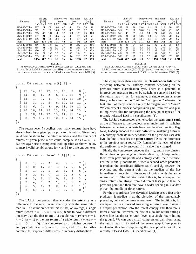
LAS LAZ SID LAZ SID LAZ SID LAZ SID5126-05-57.las 287 21 68 13.4 4.2 4.1 85 20 625126-05-58.las 312 29 80 10.6 3.9 4.7 97 22 725126-05-59.las 363 45 104 8.1 3.5 5.9 120 25 1005126-05-60.las 287 21 68 13.5 4.2 4.1 87 20 585126-05-61.las 286 21 68 13.4 4.2 4.1 87 20 58total 1,534 138 388 11.1 4.0 23 476 106 3501942-29-59.las 486 83 144 5.9 3.4 18 242 35 1561942-29-60.las 485 81 142 6.0 3.4 15 246 33 1541942-29-61.las 480 80 140 6.0 3.4 14 234 33 1531942-29-62.las 464 77 135 6.0 3.4 13 224 31 1431958-23-23.las 539 86 156 6.3 3.4 14 268 37 173total 2,454 407 716 6.0 3.4 74 1,214 169 779

TABLE IIPERFORMANCE COMPARISON BETWEEN LASZIP (LAZ) AND THE

LIZARDTECH LIDAR COMPRESSOR (SID) IN COMPRESSION RATIO AND

ENCODING/DECODING TIMES FOR LIDAR OF THE MINNESOTA DNR [5].

const U8 return_map_m[8][8] ={{ 15, 14, 13, 12, 11, 10, 9, 8 },{ 14, 0, 1, 3, 6, 10, 10, 9 },{ 13, 1, 2, 4, 7, 11, 11, 10 },{ 12, 3, 4, 5, 8, 12, 12, 11 },{ 11, 6, 7, 8, 9, 13, 13, 12 },{ 10, 10, 11, 12, 13, 14, 14, 13 },{ 9, 10, 11, 12, 13, 14, 15, 14 },{ 8, 9, 10, 11, 12, 13, 14, 15 }

};

The return level l specifies how many returns there havealready been for a given pulse prior to this return. Given onlyvalid combinations for the return number r and the number ofreturns of given pulse n we could compute it as l = n − r.But we again use a completed look-up table as shown belowto map invalid combinations for r and l to different contexts.

const U8 return_level_l[8][8] ={{ 0, 1, 2, 3, 4, 5, 6, 7 },{ 1, 0, 1, 2, 3, 4, 5, 6 },{ 2, 1, 0, 1, 2, 3, 4, 5 },{ 3, 2, 1, 0, 1, 2, 3, 4 },{ 4, 3, 2, 1, 0, 1, 2, 3 },{ 5, 4, 3, 2, 1, 0, 1, 2 },{ 6, 5, 4, 3, 2, 1, 0, 1 },{ 7, 6, 5, 4, 3, 2, 1, 0 }

};

The LASzip compressor then encodes the intensity as adifference to the most recent intensity with the same returnmap m. The intuition behind this is that, on average, a singlereturn (where r = 1, n = 1, m = 0) tends to have a differentintensity than the first return of a double return (where r = 1,n = 2, m = 1) or the last return of a triple return (where r =3, n = 3, m = 5). The compressor also switches between 4entropy contexts m = 0, m = 1, m = 2, and m > 3 to furthercorrelate the expected differences in intensity distributions.

file size compression enc. time dec. timefile name [MB] ratio [sec] [sec]

LAS LAZ LCMP LAZ LCMP LAZ LCMP LAZ LCMP5126-05-57.las 287 21 26 13.4 11.1 21 119 20 1255126-05-58.las 312 29 38 10.6 8.2 21 161 22 1495126-05-59.las 363 45 59 8.1 6.1 24 240 25 1205126-05-60.las 287 21 26 13.5 11.0 19 120 20 655126-05-61.las 286 21 26 13.4 11.1 17 122 20 65total 1,534 138 175 11.1 8.8 102 762 106 5241942-29-59.las 486 83 94 5.9 5.2 42 212 35 2761942-29-60.las 485 81 91 6.0 5.3 40 281 33 3631942-29-61.las 480 80 90 6.0 5.3 37 348 33 3551942-29-62.las 464 77 87 6.0 5.3 37 343 31 3451958-23-23.las 539 86 97 6.3 5.5 41 380 37 379total 2,454 407 460 6.0 5.3 198 1,564 169 1,718

TABLE IIIPERFORMANCE COMPARISON BETWEEN LASZIP (LAZ) AND THE

LASCOMPRESSION CODER (LCMP) [21] IN COMPRESSION RATIO AND

ENCODING/DECODING TIMES FOR LIDAR OF THE MINNESOTA DNR [5].

The compressor then encodes the classification bits whileswitching between 256 entropy contexts depending on theprevious return classification byte. There is a potential toimprove compression further by switching contexts based onthe return map m as, for example, a single return is morelikely to be classified as “building” or “ground” whereas thefirst return of many is more likely to be “vegetation” or “wire”.We can expect a modest compression gain from this and planto implement this for compressing the new point types of therecently released LAS 1.4 specification [1].

The LASzip compressor then encodes the scan angle rankas the difference to the previous scan angle rank. It switchesbetween two entropy contexts based on the scan direction flag.Next, LASzip encodes the user data while switching between256 entropy contexts in dependence on the previous user databyte, before it encodes the point source ID as the differenceto the previous point source ID. Remember that each of thesesix attributes is only encoded if its value has changed.

Finally the compressor encodes the x, y, and z coordinates.Rather than compressing coordinates directly, LASzip predictsthem from previous points and entropy codes the difference.For the x and y coordinate it uses a second order predictor:it predicts the coordinate differences dx and dy between theprevious and the current point as the median of the fiveimmediately preceding differences of points with the samereturn map m. The intuition behind this is, for example, thatsingle returns are always from a different laser pulse than theprevious point and therefore have a wider spacing in x and/ory than the middle of three returns.

For the z coordinate (the elevation) LASzip uses a first orderpredictor: it predicts z as the elevation of the immediatelypreceding point of the same return level l. The intuition is, forexample, that in a forested area a higher return level l signalsa deeper penetration into the forest canopy and therefore alower elevation. However, the first of a double return hitting apower-line has the same return level as a single return hittingthe ground. We can get a small compression gain from usingthe return map m instead of the return map l. We plan toimplement this for compressing the new point types of therecently released LAS 1.4 specification [1].

Fig. 1. The data-sets used in Tables II, III, and IV are provided by the DNR Minnesota [5]. Shown are various derivatives such as false-color elevation,standard deviation of elevation, highest intensity, hill-shaded elevation, and point densities generated with lasgrid and blast2dem from LAStools [2].

B. Compressing GPSTIME10 (version 2)

The GPS times of a single flight path are a monotonicallyincreasing sequence of double-precision floating-point num-bers where returns of the same pulse have the same GPS timeand where subsequent pulses have a more or less constantspacing in time. While the LASzip compressor is optimizedfor compressing single flight paths it will handle any GPS timesequence. The compression ratio depends on how far the inputis from the expectations. For randomly permuted points it willbe terrible. For multiple flight paths that have been sorted intotiles one after another it will be excellent.

For compression purposes LASzip treats double-precisionfloating-point GPS times as if they were signed 64 bit integersand predicts the deltas between them. As prediction contexts,it stores up to four previously compressed GPS times withcorresponding deltas. Keeping multiple prediction contextscan account for repeated jumps in GPS time that arise whenmultiple flight paths are merged with fine spatial granularity.

LASzip distinguishes several cases that are entropy codedwith 516 symbols depending on if the current GPS time is

0 predicted with a delta of zero.1–500 predicted using the current delta times 1 to 500.501–510 predicted using the current delta times -1 to -10.511 identical to the last.512 starting a new context.513–515 predicted with one of the other three contexts.

For the first three cases LASzip subsequently difference codesthe delta prediction and the actual delta. Nothing further is

coded when the GPS times are identical. LASzip starts anew context when the delta overflows a 32 bit integer. Forthat it difference codes the 32 higher bits of the current GPStime and the current context and stores the lower 32 bits raw.Otherwise it switches to the specified context (where the deltawill not overflows a 32 bit integer) and recurses. The currentdeltas stored with each context are updated to the actual deltawhen they were outside the predictable range more than 3consecutive times (i.e. bigger than 500 times the current delta,smaller than -10 times the current delta, or zero).

Currently the LASzip compressor does not make use ofknown data from the already compressed item POINT10for compressing GPSTIME10. However, if return counts andpoint source IDs are populated correctly there is significantcorrelation that can be exploited. For example, subsequentreturns of the same pulse are likely to have the same exactGPS time, and subsequent returns with different point sourceIDs are likely to require a context switch. We plan to exploitthis when compressing the new point types of the recentlyreleased LAS 1.4 specification which include the GPS time asan integral part of the point [1].

C. Compressing RGB12 (version 2)

LAS uses unsigned 16 bit integers for the R, G, and Bchannel. Some files—incorrectly—populate only the lower 8bits so that the upper 8 bits are zero. Other files—correctly—multiply 8-bit colors with 256 so that the lower 8 bits are zero.The LASzip compressor therefore compresses the upper andlower byte of each channel separately. First it entropy codes 6

bits that specify which bytes have changed as one symbol. Forall bytes that have changed it then entropy codes the differenceto the respective previous byte modulo 256.

The channels are encoded in the order R, G, and B.Differences encoded in earlier channels are used to predictdifferences in later channels as there tends to be a correlationin the intensity across channels—especially for gray colors.For example, if there was a byte difference in the low byteof the R channel that difference is added to low byte of theG channel which—clamped to a 0 to 255 range—becomesthe value to which the difference of the current low byte iscomputed.

D. Compressing WAVEPACKET13 (version 1)

The LASzip compressor supports compression of pointtypes 4 and 5 that contain wave packet information. However,the current scheme is still in version 1 as it has yet to beoptimized. So far there has been very little real-world demandfor compressing LAS files containing waveform data simplydue to a lack of data stored in this format.

LASzip simply entropy codes the wave packet descriptorindex, an unsigned byte that is zero if a point has no waveformand indexes the variable length record describing the formatof the waveform otherwise. To compress the bytes offset towaveform data it entropy encodes one of 4 possible cases:

1) same as last offset2) use last offset plus last packet size3) difference to last offset is less than 32 bits4) difference to last offset is more than 32 bits

In the first two cases no other information is needed. Forthe other two cases LASzip difference codes the 32 or the64 bit numbers. The LASzip compressor difference codedall remaining fields. Only waveform packet size in bytesis an integer number. The return point waveform location,x(t), y(t), and z(t) are single-precision floating-point numberswhose 32 bits are treated as if they were a 32-bit integer.

E. Compressing BYTE (version 2)

A LAS point may have “extra bytes” because the LASheader specifies a point size larger than required by the re-spective point type. Each “extra byte” is entropy encoded withits own context as the difference to the previous “extra byte”modulo 256. Treating them as individual bytes is currentlythe best that the LASzip compressor can do as there is nodescription in the LAS 1.3 specification what these “extrabytes” may mean. Six “extra bytes”, for example, could bea single-precision float storing the echo width followed byan unsigned short storing the normalized reflectivity. Or itcould be an unsigned short storing a tile index followed by anunsigned integer storing the original index of the point. Therecently released LAS 1.4 specification now officially has an“Extra Bytes” variable length record to describe the structureand the individual data types of “extra bytes” [1], which willallow compressing them more appropriately in the future.

20.0

40.0

60.0

80.0

100.0

5K 10K 20K 50K 75K 100K

uncompressed compressed size [MB]file name size 5 K 10 K 20 K 50 K 75 K 100 K5126-05-57.las 287 24.3 22.9 22.0 21.3 21.2 21.25126-05-58.las 312 33.4 31.5 30.2 29.4 29.1 29.15126-05-59.las 363 51.0 48.2 46.2 44.8 44.5 44.15126-05-60.las 287 24.4 22.9 22.0 21.3 21.2 21.15126-05-61.las 286 24.4 23.0 22.1 21.4 21.2 21.1total 1,534 157 149 143 138 137 1361942-29-59.las 486 93.7 88.9 85.5 82.7 82.0 81.61942-29-60.las 485 91.6 87.0 83.9 81.2 80.5 80.11942-29-61.las 480 90.2 85.7 82.6 80.0 79.3 78.91942-29-62.las 464 87.0 82.6 79.5 77.1 76.2 75.91958-23-23.las 539 96.8 92.0 88.6 85.9 85.1 84.6total 2,454 459 436 420 407 403 401

TABLE IVTHE EFFECT OF DIFFERENT CHUNK SIZES 5,000, 10,000, 20,000, 50,000,75,000, AND 100,000 POINTS ON THE COMPRESSION RATES OF LASZIP.

IV. RESULTS

All timings were taken on an old (2005) Dell InspironD6000 laptop with a 2.13 Ghz Intel processor and an evenolder (2003) external LaCie 120 GB fire-wire drive. Encodetimings include reading the uncompressed LAS file fromthe local disk (the disk cache was flushed) and writing thecompressed LAZ file to the external fire-wire disk. Decodetimings include reading the compressed LAZ file from the

LiDAR of Minnesota DNR by county size [GB] compressionname # of files # of points LAS LAZ ratiocottonwood 216 2,491,327,766 65.0 5.2 12.6douglas 252 2,092,702,039 54.6 5.4 10.2freeborn 260 1,713,544,294 44.7 3.7 12.1houston 197 1,450,109,156 37.8 3.9 9.8jackson 240 2,724,531,642 71.0 5.6 12.6lincoln 195 2,200,533,847 57.4 4.5 12.8martin 252 2,853,353,232 74.4 5.8 12.9murray 252 2,872,608,269 74.9 5.8 12.9pope 247 2,404,624,049 62.7 5.3 11.9redwood 302 3,505,060,711 91.4 7.3 12.4sibley 219 2,501,934,963 65.2 5.8 11.2swift 282 2,931,687,204 76.4 5.8 13.2total 2,914 29,742,017,172 776 64 12.1

TABLE VLASZIP COMPRESSES 30 BILLION POINTS (OR 12 COUNTIES WORTH OF

LIDAR) FROM 776 GB OF LAS DOWN TO 64 GB OF LAZ FOR LIDARHOSTED BY THE DNR OF MINNESOTA AT FTP://LIDAR.DNR.STATE.MN.US.

external fire-wire disk and writing the uncompressed LAS fileback to the local disk. Reading and writing from differentdisks makes the process less I/O bound. Nevertheless, the CPUusage for LASzip averages only 50% to 70% on this laptop.When decompressing LAZ files into memory (not measuredhere) LASzip is entirely CPU-bound running at 99%.

The most common question about LASzip is how it com-pares to the LizardTech R© LiDAR compressorTM that gen-erates the well-known MrSID format [20]. The results inTable II show a comparison of the two compressors in termsof compression ratio, encoding speed, and decoding speedon typical LiDAR tiles that are publicly provided by theMinnesota Department of Natural Resources [5]. LASzip isa clear winner over MrSID in all three performance measures.The compressed LAZ files are 2 to 3 times smaller than thecompressed SID files, compression was 16 to 20 times faster,and decompression was 3 to 4 times faster. The encode (!)times were taken at the Minnesota DNR on a Dell PrecisionT3400 workstation with a 3.14 Ghz Intel processor. The de-code times were taken on the Dell laptop using the command-line lidardecode.exe version 1.1.0.2802 [20].

We need to be a bit careful in comparing LASzip andthe LizardTech LiDAR compressor because they are aimedat different work-flows: LASzip is designed to turn large LASfiles into more compact LAZ files for easier management,faster transmission, and lower file system I/O. The LizardTechproduct adds extra value by seamlessly integrating into theestablished raster work-flow of the MrSID file format andincludes multi-resolution support for fast access to the pointdata at global scale with an option for lossy compression.

In Table III we compare the performance of LASzip with theLASCompression software [21] that implements the algorithmdescribed by Mongus and Zalik [22] on the exact same data-sets. LASzip consistently achieves between 15 to 25 percenthigher compression, encodes 7 to 8 times faster, and decodes5 to 10 times faster. These are end-to-end wall-clock timingstaken under the exact same conditions for I/O performance ofthe laptop / fire-wire disk configuration. While compressionrates are comparable, LASzip clearly excels in speed.

The impact of different chunk sizes on the achieved com-pression is illustrated in Table IV. Smaller chunk sizes meanless compression as the adaptive entropy coder resets at thestart of each chunk and needs to relearn all symbol distribu-tions, which negatively affects compression. There is little tobe gained from chunk sizes larger than 50,000 and there is noreason for choosing chunk sizes smaller than 5,000 as LiDARis usually processed in increments of millions of points.

A large-scale user of LASzip is the Department of NaturalResources of Minnesota that—at the time of writing—hosts40 counties of publicly accessible LiDAR in LAZ format [5].An overview of the savings in data storage, transmission band-width, and download time for 12 of those counties is detailedin Table V. The 30 billion points that would take up 776 GBif stored as LAS files compress down to 64 GB as LAZ.

Compression performance across a large smorgasbord oftypical, experimental, as well as unusual LAS files is reported

in Table VI with the number corresponding to the smallest filesize (or the highest compression ratio) being in bold. We alsoreport the point type and loosely categorize the point order asboth have an effect on the compression rates. Point order fmeans in flight-line order, point order x means sorted alongsome axis, and point order t means some form of tiling.

The standard WinZIP algorithm is by far the worst per-former. This is noteworthy because WinZIP is still used byseveral agencies to provide compressed LAS downloads. Incontrast, the generic WinRAR algorithm does surprisinglywell. While it takes a long time to compress, in terms ofcompression rate it gives the dedicated LizardTech LiDARcompressor a run for its money. The LT compressor struggleswith point types 1 and 3 that contain an 8 byte floating-pointGPS time, which it compresses with the inefficient DEFLATE.

Again, LASzip gives the overall best compression ratio.The data sets on which it is outperformed are usually thosesorted along an axis (i.e. point order x) or those with littleoddities such as “Grass Lake Small”, for example, which hasrandom values in its return number field and its classificationfield or “line 27007 dd”, which has a strange z coordinatescaling. Although not reported here, LASzip is across theboard the—by far—fastest algorithm for both compression anddecompression.

V. DISCUSSION

Compressing LAS with WinZIP, WinRAR, gzip, bzip, orany other generic compressor not only means settling for largerfiles and slower encoding and decoding speeds, but also meansthat no seeking is possible in the compressed file and thataccessing any part of the LiDAR requires to completely de-compress the file first. LASzip allows you to treat compressedLAZ files just like standard LAS files. You can load themdirectly from compressed form into your application withoutneeding to decompress them onto disk first. The availability oftwo APIs, LASlib [2] and libLAS [3], with LASzip capabilitymakes it easy to add native LAZ read/write support to yourown software package. The LASzip source code is availableon the website indicated above.

The LASzip compressor is optimized for the case wherepoints are stored more or less in scanner acquisition order inthe LAS file and the compression rates degrades the fartherthe file is from that assumption. If a LAS file is a tile that ispart of a larger tiling, the best compression rates are achievedwhen the flight-lines that pass through the tile are kept inacquisition order (e.g. like lastile from LAStools does it).Some LiDAR processing software disturbs the original pointorder and produces seemingly meaningless point permutations.When compressing large LiDAR collects to be offered via aweb server to a large audience it may make sense to first re-order the points of each tile into acquisition order (e.g. withlassort from LAStools).

The compressed LAZ files can - just like the original LASfiles - be used in conjunction with the small spatial indexingLAX files (that can be produced with lasindex). Thissupports efficient area-of-interest queries when reading the

original LAS file point compression ratio total file size in MBname size in bytes type order ZIP RAR LCMP SID LAZ LAS ZIP RAR LCMP SID LAZGrass Lake Small 123,876,781 0 x 2.6 6.1 7.0 6.9 6.2 118 46 19 17 17 19LASFile 1 48,097,847 0 f 1.9 3.8 4.8 4.3 4.8 46 24 12 10 11 10LASFile 2 44,168,907 0 f 1.9 3.8 4.9 4.5 4.9 42 22 11 9 9 9LASFile 3 16,782,887 0 f 1.8 3.6 4.6 4.2 4.7 16 9 4 3 4 3LASFile 4 48,471,887 0 f 1.9 3.9 4.9 4.5 5.0 46 24 12 9 10 9LDR030828 212242 0 59,672,207 0 f 1.9 3.8 4.8 4.4 4.9 57 30 15 12 13 12LDR030828 213023 0 58,414,787 0 f 1.9 3.8 4.8 4.5 5.0 56 29 15 12 12 11LDR030828 213450 0 53,215,067 0 f 1.9 3.8 4.8 4.3 4.9 51 27 13 11 12 10Lincoln 185,565,975 0 x 1.7 6.1 6.1 6.1 6.5 177 106 29 29 29 27line 27007 dd 107,603,879 0 x 2.4 3.5 3.6 4.0 3.8 103 42 30 28 26 27MARS Sample Filtered LiDAR 163,225,753 0 x f t 2.8 6.5 7.1 6.3 8.3 156 56 24 22 25 19Mount St Helens Nov20 2004 115,737,877 0 x 2.2 12.4 13.4 12.9 12.6 110 51 9 8 9 9Mount St Helens Oct4 2004 134,868,035 0 x 1.7 6.1 6.7 6.4 6.6 129 78 21 19 20 19ncwc000008 63,161,789 0 f t 1.8 3.1 3.5 3.1 3.4 60 34 19 17 19 18Palm Beach Pre Hurricane 51,612,715 0 x 1.6 6.6 7.0 6.5 6.8 49 30 7 7 8 7Dallas 104,639,368 1 f t 1.8 5.2 6.2 2.8 7.5 100 55 19 16 36 13IowaDNR-CloudPeakSoft-1.0-UTM15N 163,727,279 1 f t 2.5 8.8 8.3 3.3 11.2 156 62 18 19 47 14LDR091111 181233 1 54,609,113 1 f 1.8 4.4 5.1 2.8 5.6 52 29 12 10 19 9LDR091111 182803 1 54,255,417 1 f 1.8 4.5 4.9 2.8 5.7 52 28 12 11 19 9merrick vertical 1.2 54,609,113 1 f 1.8 4.4 5.1 2.8 5.6 52 29 12 10 19 9S1C1 strip021 78,220,943 1 f 2.0 6.2 7.8 3.4 8.4 75 37 12 10 22 9Serpent Mound Model LAS Data 91,423,839 1 f 2.2 5.6 6.9 3.3 8.8 87 40 15 13 27 10Tetons 104,800,536 1 f t 2.0 4.8 5.0 2.8 6.0 100 50 21 20 35 17USACE Merrick lots of VLRs 101,081,369 1 f t 1.8 4.6 5.2 2.9 5.5 96 54 21 19 33 18LAS12 Sample withRGB Quick Terrain Modeler 99,156,855 2 x 2.7 6.5 error 6.5 7.4 95 35 14 error 15 13xyzrgb manuscript 56,046,269 2 t 2.9 8.5 10.2 9.7 10.9 53 18 6 5 5 5autzen-colorized-1.2-3 362,213,959 3 f t 2.1 2.3 5.2 3.1 6.6 345 164 148 66 119 52total 2,599,260,453 2.0 4.5 5.9 4.1 6.4 2,479 1,210 551 425 610 388

TABLE VICOMPRESSION PERFORMANCE BETWEEN WINZIP (ZIP), WINRAR (RAR), LASCOMPRESSION (LCMP), THE LIZARDTECH LIDAR COMPRESSOR

(SID), AND LASZIP (LAZ) FOR TYPICAL, EXPERIMENTAL, AS WELL AS UNUSUAL LAS FILES THAT ARE AVAILABLE AT HTTP://LIBLAS.ORG/SAMPLES.

LAS/LAZ files with any LAStools tool or any application thatuses the LASlib API [2] to read or write LAS or LAZ files.

ACKNOWLEDGMENT

The author would like to thank those who have down-loaded “LAStools” and sent useful feature requests or bugreports, Howard Butler for suggesting “chunking”, and TimLoesch from the DNR Minnesota for the first large-scaleLAZ campaign. Financial support for version 2.0 of LASzipwas provided by Dave Finnegan from USACE Cold RegionsResearch and Engineering Laboratory and by Hobu Inc. inconjunction with other open source efforts it operates includinglibLAS and PDAL. Michael P. Gerlek from Flaxen Geo andHoward Butler from Hobu Inc. assisted with the integrationof LASzip versions 1.0 and 2.0 into libLAS.

REFERENCES

[1] ASPRS LAS format, “Specifications for the LASer exchange fileformat,” accessed on November 21th 2011. [Online]. Available:http://www.asprs.org/LAS Specification

[2] LAStools, “Efficient tools for LiDAR processing.” [Online]. Available:http://www.lastools.org/

[3] libLAS, “A LAS 1.0/1.1/1.2 ASPRS LiDAR data translation toolset.”[Online]. Available: http://www.liblas.org/

[4] OpenTopography, “A portal to high-resolution topography data andtools.” [Online]. Available: http://www.opentopography.org/

[5] Minnesota Department of Natural Resources, “Minnesota state LiDARcollect.” [Online]. Available: ftp://lidar.dnr.state.mn.us/

[6] M. Isenburg, P. Lindstrom, and J. Snoeyink, “Lossless compressionof predicted floating-point geometry,” Computer-Aided Design, vol. 37,no. 8, pp. 869–877, 2005.

[7] M. Deering, “Geometry compression,” in SIGGRAPH 95 ConferenceProceesings, 1995, pp. 13–20.

[8] C. Touma and C. Gotsman, “Triangle mesh compression,” in GraphicsInterface’98 Proceedings, 1998, pp. 26–34.

[9] G. Taubin and J. Rossignac, “Geometric compression through topologi-cal surgery,” ACM Transactions on Graphics, 17 (2), pp. 84–115, 1998.

[10] O. Devillers and P.-M. Gandoin, “Geometric compression for interactivetransmission,” in Proc. of IEEE Visualization 2000, 2000, pp. 319–326.

[11] M. Isenburg and S. Gumhold, “Out-of-core compression for giganticpolygon meshes,” in SIGGRAPH 2003 Proceedings, 2003, pp. 935–942.

[12] J. Peng and C. C. Kuo, “Geometry-guided progressive lossless 3dmesh coding with octree (OT) decomposition,” in SIGGRAPH ’05Proceedings, 2005, pp. 609–616.

[13] M. Isenburg, P. Lindstrom, and J. Snoeyink, “Streaming compressionof triangle meshes,” in Proceedings of the 3rd Symposium on GeometryProcessing, 2005, pp. 111–118.

[14] O. Devillers and P.-M. Gandoin, “Progressive and lossless compressionof arbitrary simplicial complexes,” in SIGGRAPH’2002, pp. 372–379.

[15] M. Botsch, A. Wiratanaya, and L. Kobbelt, “Efficient high qualityrendering of point sampled geometry,” in Eurographics RenderingWorkshop, 2002, pp. 53–64.

[16] R. Schnabel and R. Klein, “Octree-based point-cloud compression,” inEurographics Symposium on Point-Based Graphics, 2006, pp. 111–120.

[17] M. Waschbusch, M. Gross, F. Eberhard, E. Lamboray, and S. Wurmlin,“Progressive compression of point-sampled models,” in EurographicsSymposium on Point-Based Graphics, 2004, pp. 95–102.

[18] S. Gumhold, Z. Karni, M. Isenburg, and H. P. Seidel, “Predictive point-cloud compression,” in SIGGRAPH ’05 Sketches, 2005, p. 137.

[19] B. Merry, P. Marais, and J. Gain, “Compression of dense and regularpoint clouds,” Computer Graphics Forum, 25 (4), pp. 709–716, 2006.

[20] LizardTech R©, “LiDAR compressorTM,” accessed on October 17th 2011.[Online]. Available: http://www.lizardtech.com/

[21] LASCompression, “A lossless compression algorithm for LiDARdatasets,” accessed on November 19th 2011. [Online]. Available:http://gemma.uni-mb.si/lascompression/

[22] D. Mongus and B. Zalik, “Efficient method for lossless LiDAR datacompression,” International Journal of Remote Sensing, vol. 32, pp.2507–2518, May 2011.

[23] A. Moffat, R. M. Neal, and I. H. Witten, “Arithmetic coding revisited,”ACM Transactions on Information Systems, 16 (3), pp. 256–294, 1998.

[24] A. Said, “Fastac: Arithmetic coding implementation,” ac-cessed on October 30th 2009. [Online]. Available:http://www.cipr.rpi.edu/ said/FastAC.html