LOCO and JPEG-LSA new method for lossless and

near losslessimage compression

Nimrod PelegUpdate: May 2009

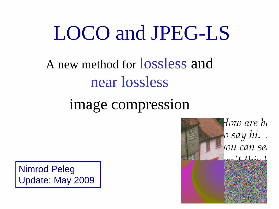
Credit...• Suggested by HP Labs, 1996• Developed by: M.J. Weinberger, G. Seroussi

and G. Sapiro,

“LOCO-I: A Low Complexity, Context-Based, Lossless Image Compression Algorithm”,

IEEE Proceedings of Data Compression Conference, pp. 140-149, 1996

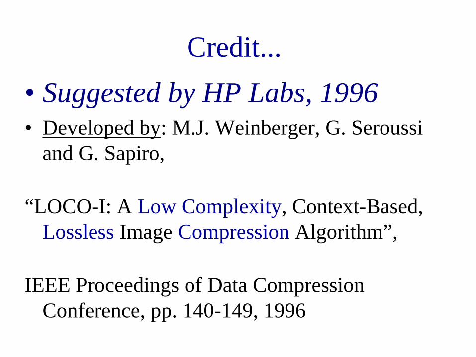
General Block Diagram

Context Modeling

Prediction

Run Mode

ErrorEncoding

Digital SourceImage Data

CompressedData

Context Based Algorithm

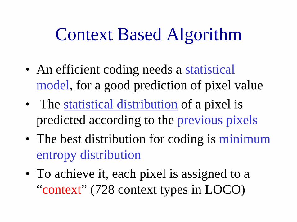
• An efficient coding needs a statistical model, for a good prediction of pixel value

• The statistical distribution of a pixel is predicted according to the previous pixels

• The best distribution for coding is minimum entropy distribution

• To achieve it, each pixel is assigned to a “context” (728 context types in LOCO)

Prediction

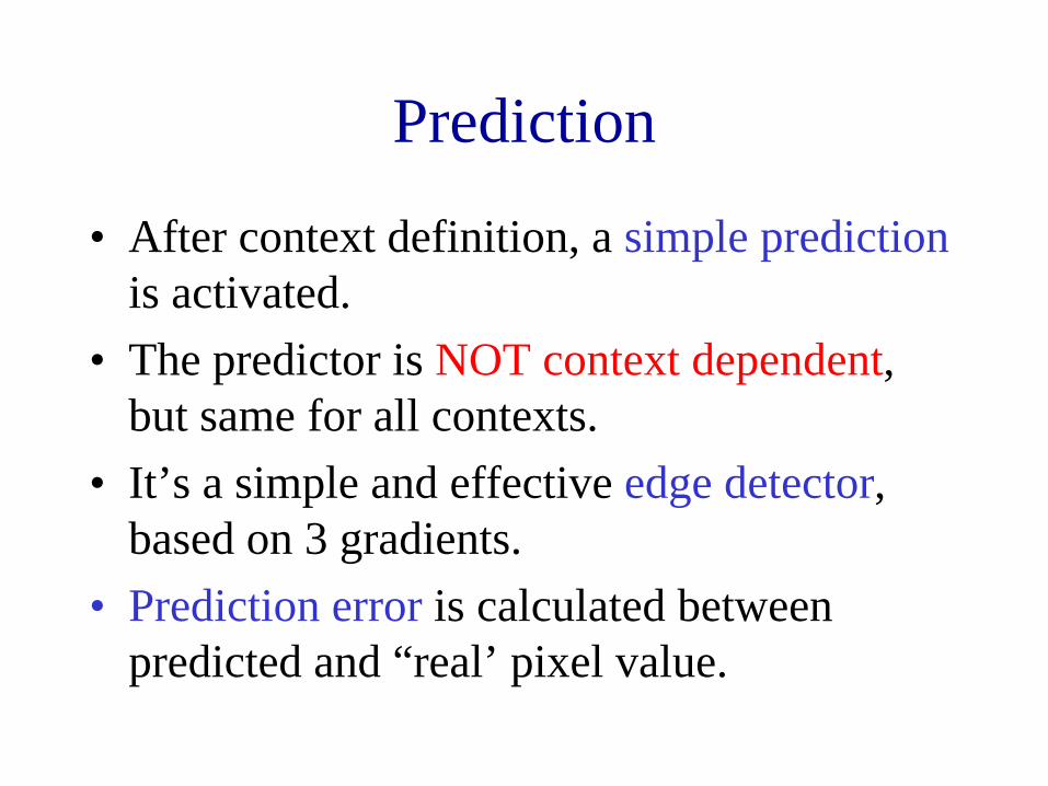
• After context definition, a simple predictionis activated.

• The predictor is NOT context dependent, but same for all contexts.

• It’s a simple and effective edge detector, based on 3 gradients.

• Prediction error is calculated between predicted and “real’ pixel value.

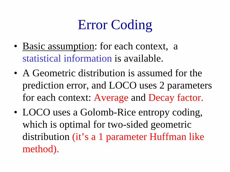
Error Coding• Basic assumption: for each context, a

statistical information is available.• A Geometric distribution is assumed for the

prediction error, and LOCO uses 2 parameters for each context: Average and Decay factor.

• LOCO uses a Golomb-Rice entropy coding, which is optimal for two-sided geometric distribution (it’s a 1 parameter Huffman like method).

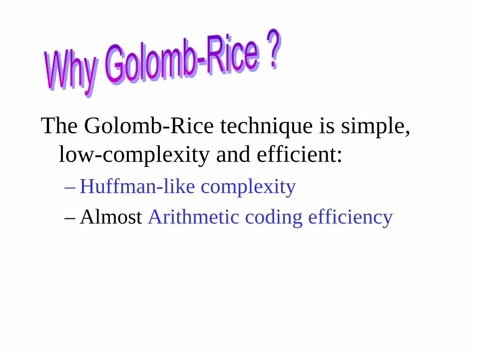
The Golomb-Rice technique is simple, low-complexity and efficient:– Huffman-like complexity– Almost Arithmetic coding efficiency

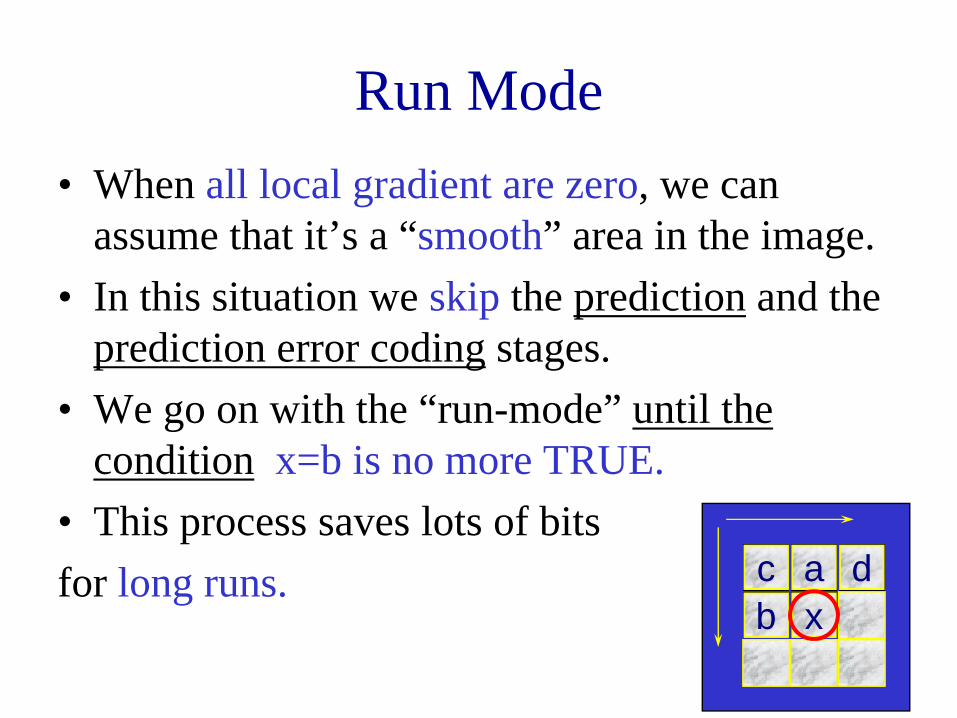
Run Mode• When all local gradient are zero, we can

assume that it’s a “smooth” area in the image.• In this situation we skip the prediction and the

prediction error coding stages.• We go on with the “run-mode” until the

condition x=b is no more TRUE.• This process saves lots of bitsfor long runs. c a d

b x

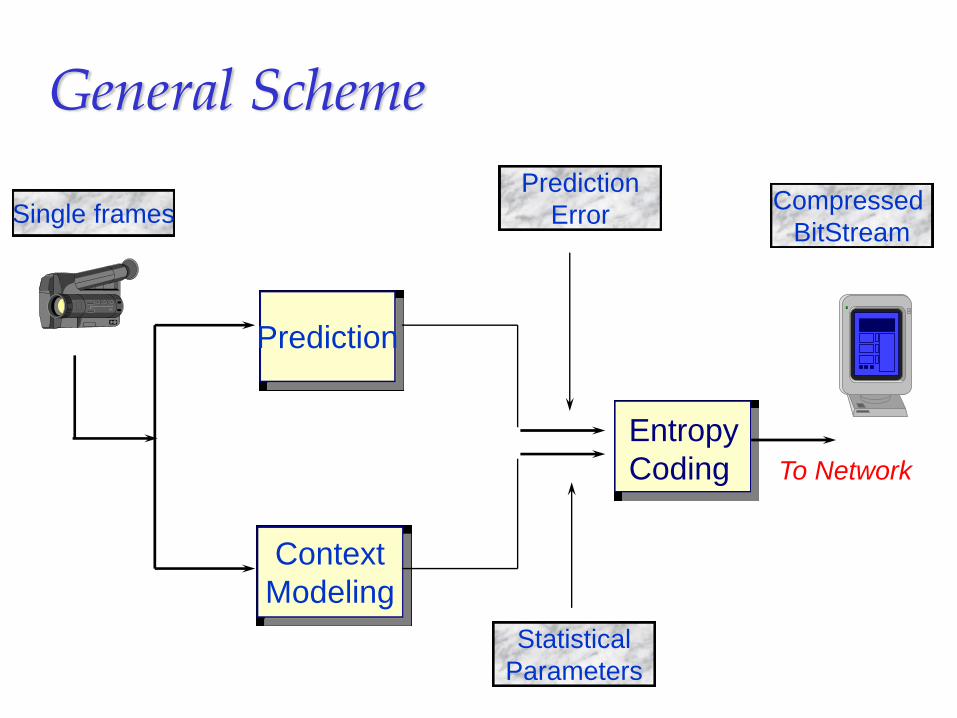
General Scheme

ContextModeling

Entropy Coding

Single framesPrediction

Error

StatisticalParameters

To Network

Compressed BitStream

Prediction

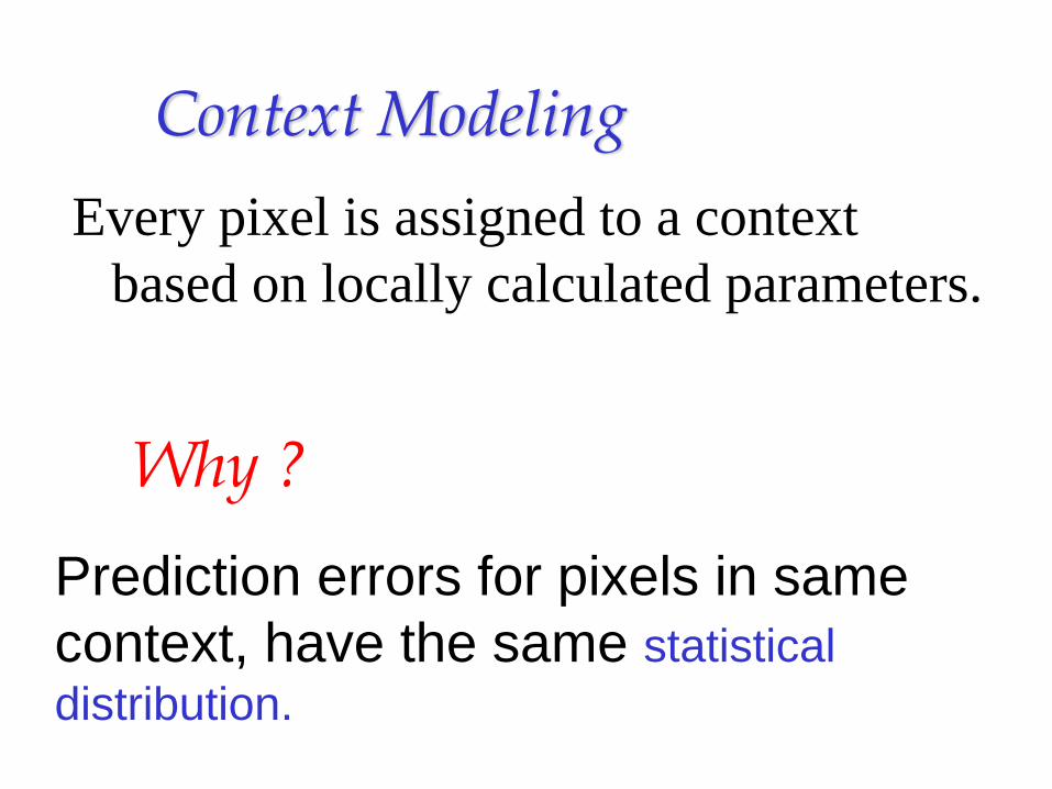
Every pixel is assigned to a context based on locally calculated parameters.

Context Modeling

Why ?

Prediction errors for pixels in same context, have the same statistical distribution.

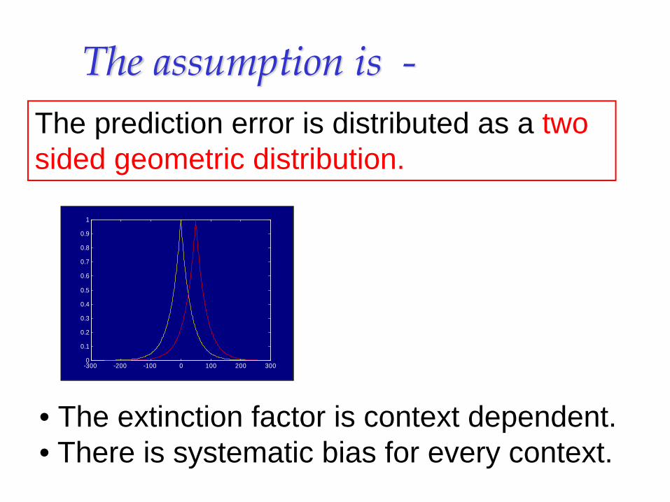
The assumption is -The prediction error is distributed as a two sided geometric distribution.

-300 -200 -100 0 100 200 3000

0.1

0.2

0.3

0.4

0.5

0.6

0.7

0.8

0.9

1

• The extinction factor is context dependent.• There is systematic bias for every context.

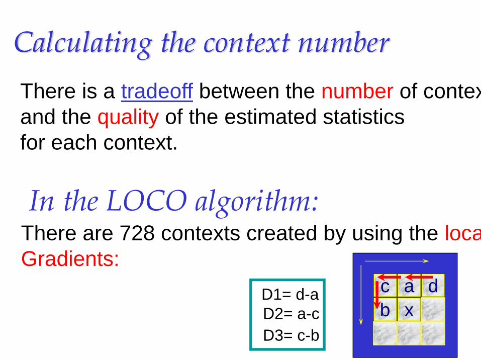
Calculating the context numberThere is a tradeoff between the number of contexand the quality of the estimated statistics for each context.

In the LOCO algorithm:There are 728 contexts created by using the locaGradients:

D1= d-aD2= a-cD3= c-b

c a db x

Prediction

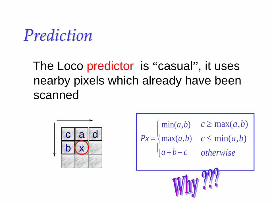
The Loco predictor is “casual”, it uses nearby pixels which already have been scanned

Pxa ba b

a b c=

+ −

⎧

⎨⎪

⎩⎪

min( , )max( , )

c a bc a botherwise

≥≤

max( , )min( , )c a d

b x

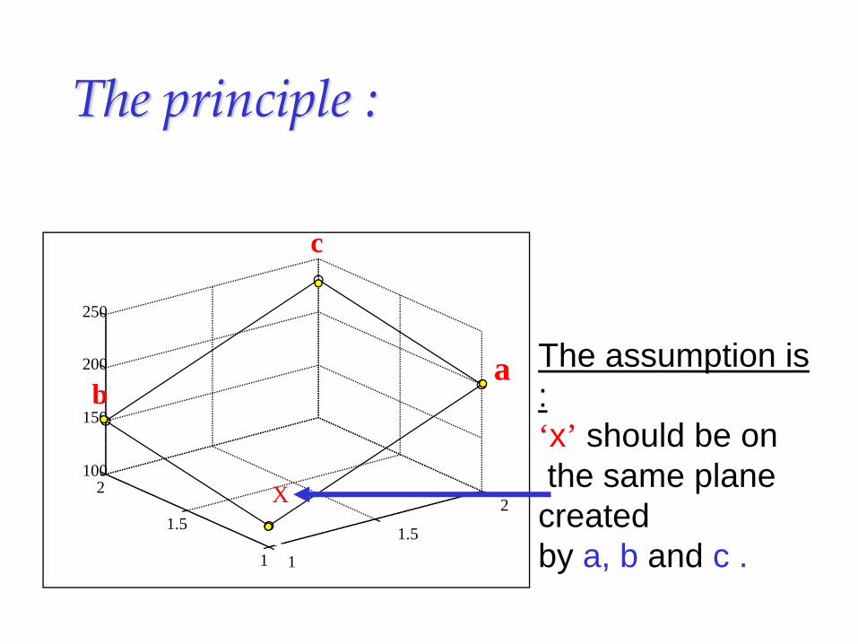
The principle :

1

1.5

2

1

1.5

2100

150

200

250

X

a

c

b

x

The assumption is :‘x’ should be onthe same plane created by a, b and c .

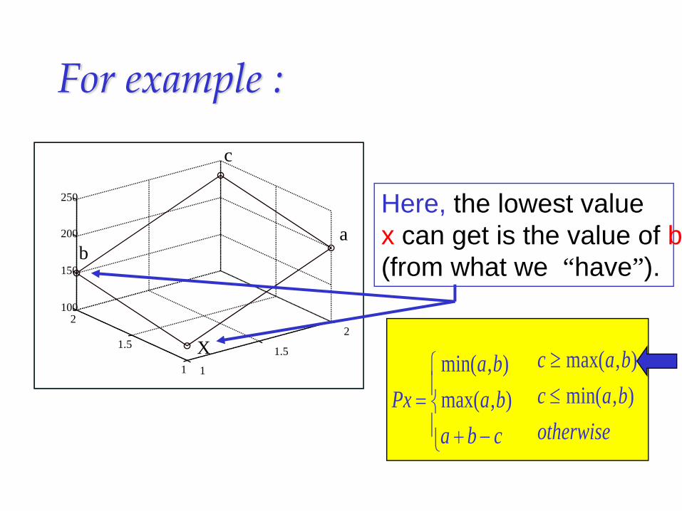
For example :

1

1.5

2

1

1.5

2100

150

200

250

c

ba

X

Here, the lowest value x can get is the value of b(from what we “have”).

Pxa ba b

a b c=

+ −

⎧

⎨⎪

⎩⎪

min( , )max( , )

c a bc a botherwise

≥≤

max( , )min( , )

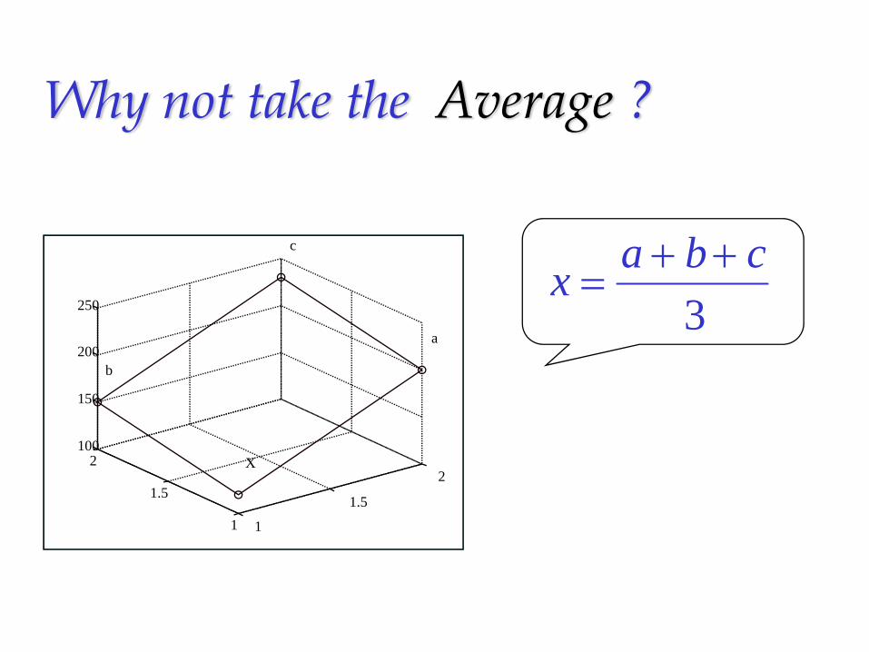
Why not take the Average ?

1

1.5

2

1

1.5

2100

150

200

250

c

b

a

X

x a b c=

+ +3

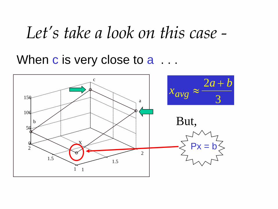
Let’s take a look on this case -When c is very close to a . . .

11.5

2

1

1.5

20

50

100

150

c

b

a

X

x a bavg ≈

+23

Px = b

But,

Original Image Predicted Image (SNR=25.3dB

Prediction Example

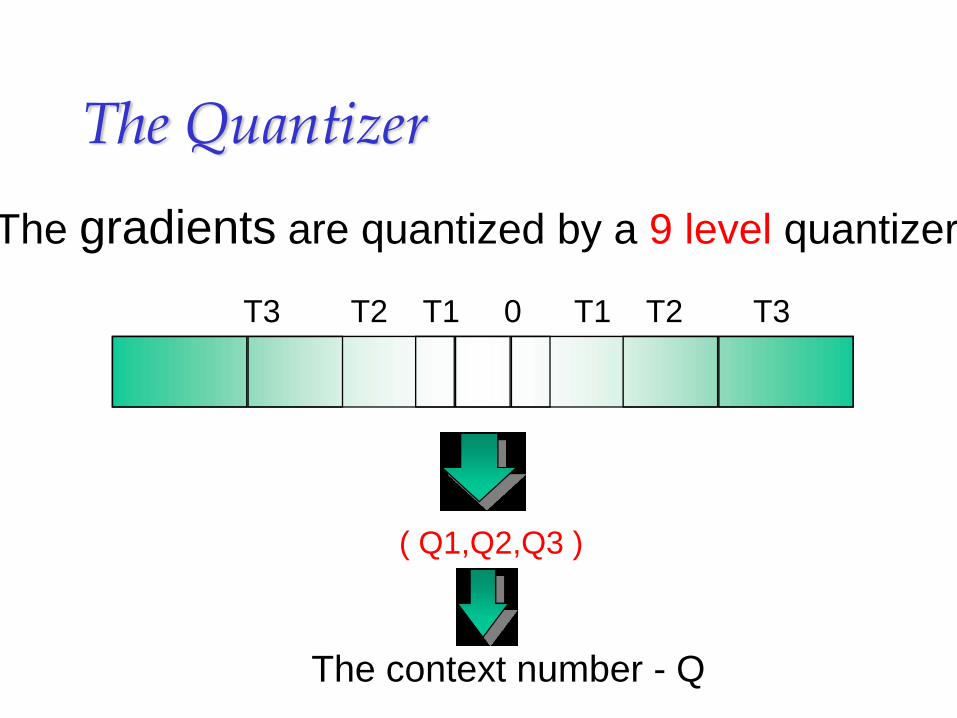
The Quantizer

The gradients are quantized by a 9 level quantizer

T3 T2 T1 0 T1 T2 T3

( Q1,Q2,Q3 )

The context number - Q

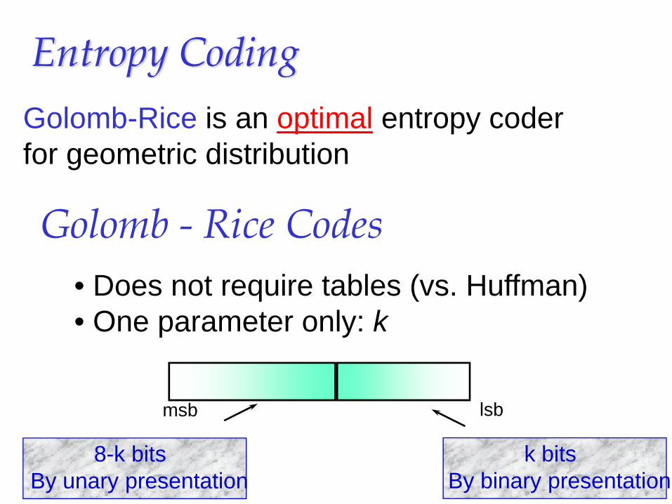
Entropy CodingGolomb-Rice is an optimal entropy coder for geometric distribution

Golomb - Rice Codes• Does not require tables (vs. Huffman)• One parameter only: k

msb

k bitsBy binary presentation

8-k bitsBy unary presentation

lsb

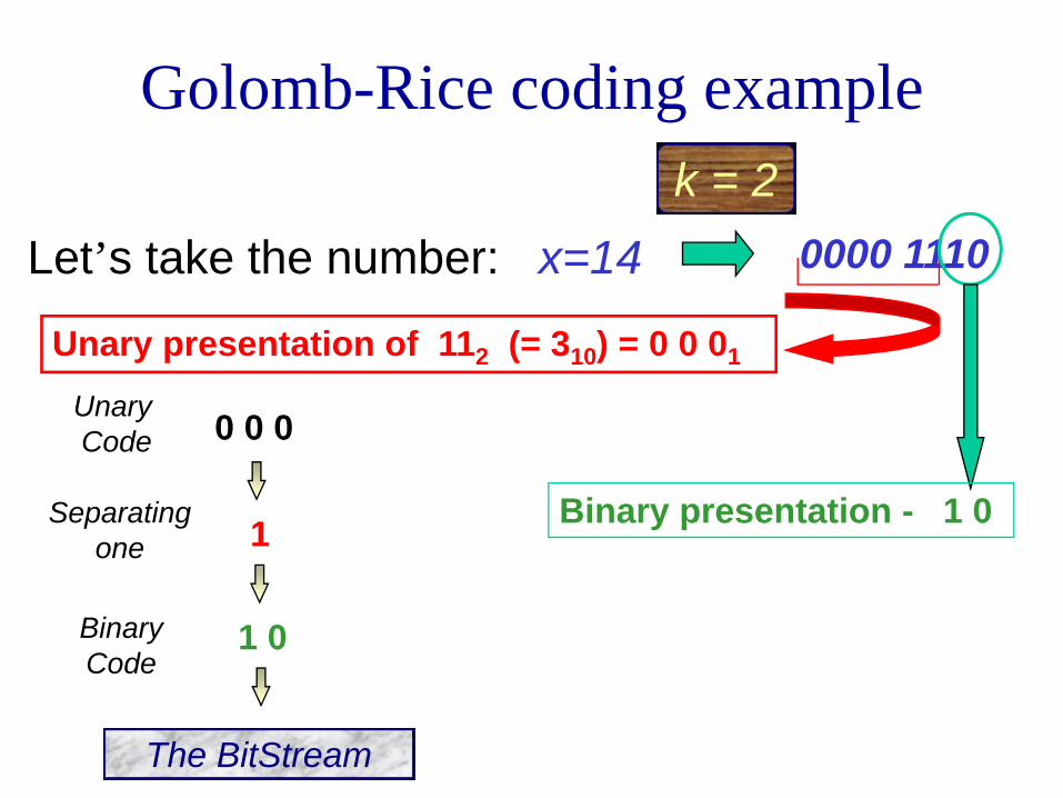
Golomb-Rice coding example

Let’s take the number: x=14 0000 1110

Unary presentation of 112 (= 310) = 0 0 01

Binary presentation - 1 0

The BitStream

UnaryCode 0 0 0

k = 2

1Separatingone

1 0BinaryCode

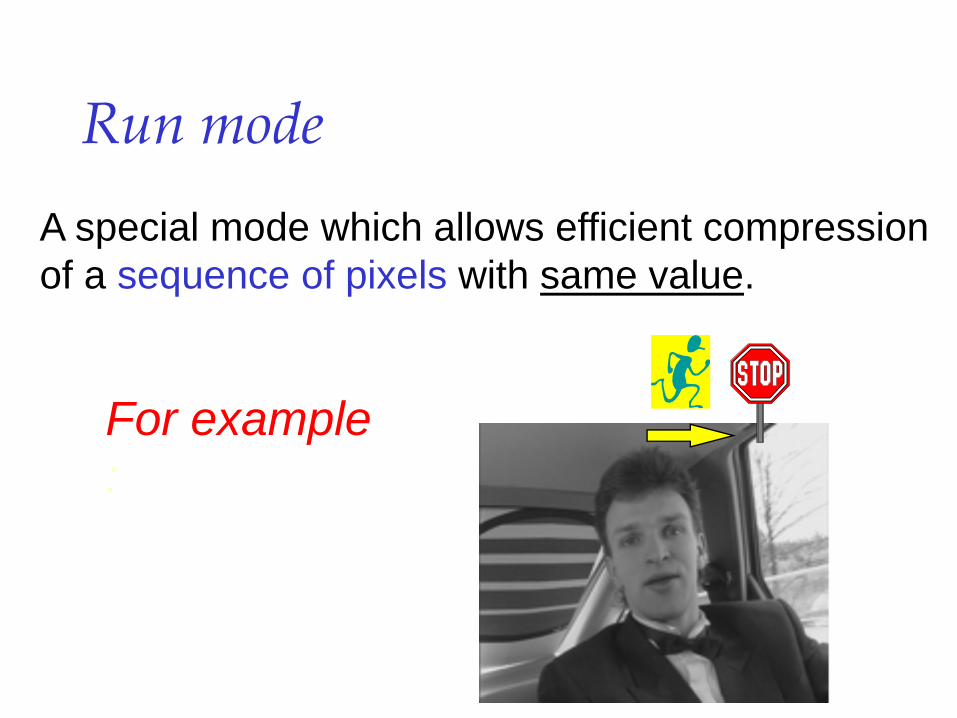
Run modeA special mode which allows efficient compressionof a sequence of pixels with same value.

For example:

Lossy Mode

Maximal allowed restoration error per pixel =0

In Lossy Mode

NEAR

The method :The prediction error is quantized by a 2Near + 1step quantizer .

Prediction Error Prediction Error2Near + 1

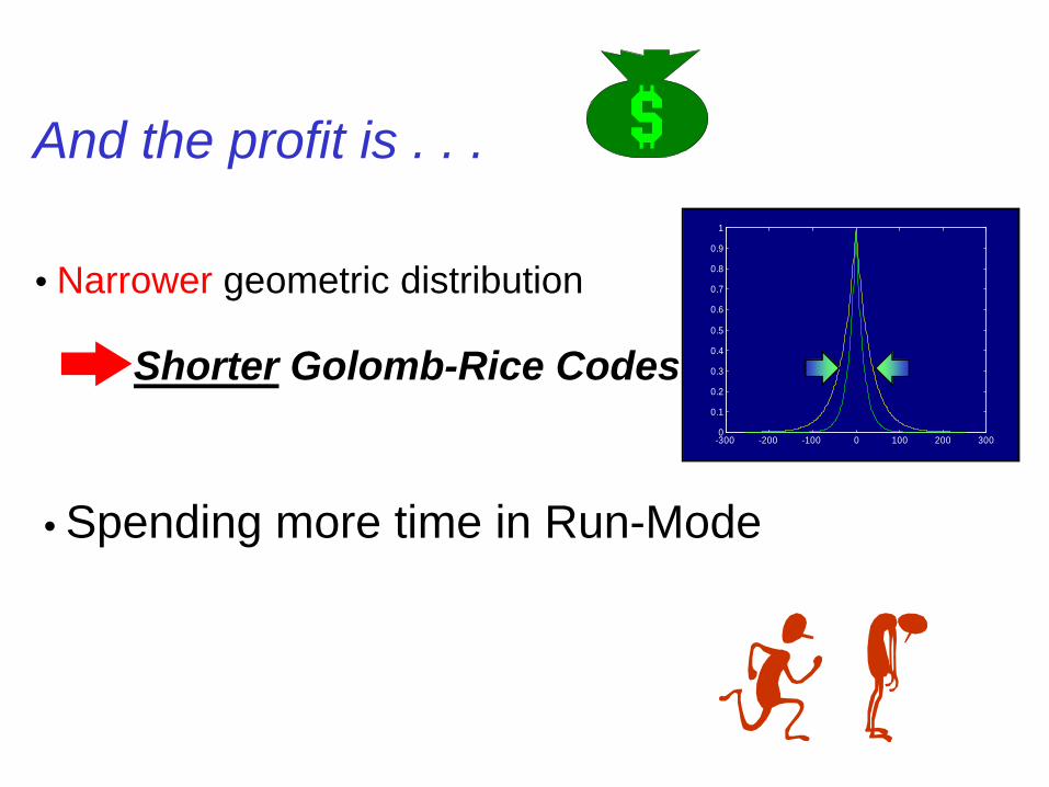
And the profit is . . .

• Narrower geometric distribution

-300 -200 -100 0 100 200 3000

0.1

0.2

0.3

0.4

0.5

0.6

0.7

0.8

0.9

1

Shorter Golomb-Rice Codes

• Spending more time in Run-Mode

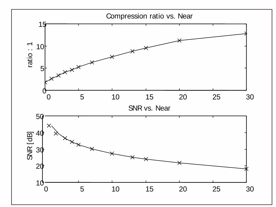
0 5 10 15 20 25 300

5

10

15Compression ratio vs. Near

ratio

: 1

0 5 10 15 20 25 3010

20

30

40

50SNR vs. Near

SNR [

dB]

Explanation (last graph: Lena for different Near values)

שבערכים נמוכים העלייה ביחס הדחיסה , ניתן לראות Nearאולם בערכים גבוהים של , Nearליניארית עם

היא , הסיבה לכך. כמעט ואין שיפור ביחס הדחיסה, גבוהים Nearבערכי Contextsמאבד את ה LOCOשה

גם איכות התמונה הדחוסה . ולכן מאבד את יעילותוכפי שניתן לראות מגרף , בערכים הגבוהים ירודה ביותר

.SNRה

Different Near values compression

Near = 3 Near = 10

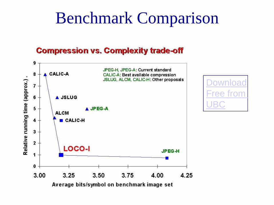
Benchmark Comparison

DownloadFree from UBC