Lasers PH 645/ OSE 645/ EE 613

Summer 2011 Section 1: T/Th 2:45- 4:45 PM Engineering Building 240

John D. Williams, Ph.D.

Department of Electrical and Computer Engineering

406 Optics Building - UAHuntsville, Huntsville, AL 35899

Ph. (256) 824-2898 email: williams@eng.uah.edu

Office Hours: Tues/Thurs 1:30-2:30PM

JDW, ECE Summer 2010

Chapter 1: Introduction to the LASER • Acronym for Light Amplification by a Stimulated Emission of Radiation

• Makes use of processes that increase of amplify light signals after those signals have been generated by other means

• Laser consist of a amplifying medium in which stimulated emission occurs and a set of mirrors to feed the light back into the amplifier for continued growth of the developing beam

http://en.wikipedia.org/wiki/Laser

LASER Process Requirements • Processes include:

– Stimulated emission: process by which an electron perturbed by a photon of the correct energy may drop to a lower energy state resulting in the creation of another photon.

http://kottan-labs.bgsu.edu/teaching/workshop2001/chapter4a.htm

– Optical feedback: occurs when a reflected light constructively interferes with itself resulting in amplification of the optical intensity.

http://prn1.univ-lemans.fr/prn1/siteheberge/optique/M1G1_FBalembois_ang/co/Contenu_05.html

Applications of the laser

• Typical laser properties include: narrow frequency bandwidth, high intensity, short pulse duration, highly collimated coherent source.

• Lasers are used only in applications in which its unique properties are required

• Blue ray/DVD players, check out scanners, surveying instruments, surgical cutting, laser drilling and cutting, communication signals

Green laser pointer

Laser Spectrum and Wavelengths

Weber, Marvin J. Handbook of laser wavelengths, CRC Press, 1999. ISBN 0-8493-3508-6

http://www.lexellaser.com/techinfo_wavelengths.htm See also, Lexel laser Corporation’s website for various commercial lasers

History of the laser

• 1887: Photoelectric effect discovered by Hertz, allowing Albert Einstein to introduce the notion of photons.

• 1901: “The ultraviolet catastrophe” (spectral energy densities diverge at high frequencies) is solved by Planck. He hypothesises that the energy of a type of frequency ν is not a random continuous variable but a random discrete set of variables, represented by the values nh ν. Interestingly, Planck and his contemporaries at first find it very difficult to accept this idea of discrete leaps in energy. However, subsequent experiments prove that the theory is entirely correct.

• 1905: Einstein introduces a means to quantify electromagnetic energy. The photon is born. Unfortunately, the arrival of the photon cannot take into account the phenomenon of black body radiation (the spectral density of electromagnetic energy emitted by an enclosed area at a temperature T and at thermal equilibrium). However, shortly afterwards, Born devises a means to quantify the energy levels of electrons (1913). This in turn allows Einstein to prove that photons and black body radiation are in fact compatible thanks to the notion of stimulated emission.

• 1949: Kastler and Brossel develop the first optical pumping and the first population inversion. By 1950, the first MASERs appear (Microwave Amplification by Stimulated Emission Radiation), devices that are capable of amplifying an electromagnetic wave in the microwave region (Weber, Townes and Basov).

http://prn1.univ-lemans.fr/prn1/siteheberge/optique/M1G1_FBalembois_ang/co/Module_M1G1_anglais.html

History of the laser (2) • 1954: The first MASER is built (an ammonia maser with a 13 mm wavelength). The electromagnetic wave is

confined in three dimensions by a “box” and is reflected off its sides. However, this is still in the microwave rather than the optical domain. In fact, scientists at the time thought it was impossible to make an optical laser because the cavity would have to be incredibly small (of the order of magnitude of a wavelength i.e. only tens of μm at the most!).

• 1958: Schawlow and Townes decide to use an open Fabry-Pérot cavity for their experiments. The idea is to confine the electromagnetic field like in a closed box but in only one dimension: the main axis of light propagation in the cavity. This means that only certain specific electromagnetic waves are amplified, but the resulting beam is much more powerful than when using a closed cavity.

• 16th May 1960: Maiman demonstrates the first ever optical laser effect. The amplifying medium is a ruby, the crystal most used in early lasers because it was already well known from its application in MASERs. This is a pulsed operation laser with a wavelength of 694.3 nm.

• 1961: Javan, Bennet and Herriot build the first gas helium-neon laser operating continuously at 1.15 . In fact, this laser can emit over a whole range of discrete wavelengths, from green to infrared via orange and red (633 nm).

http://prn1.univ-lemans.fr/prn1/siteheberge/optique/M1G1_FBalembois_ang/co/Module_M1G1_anglais.html

History of the laser (3) • 1962: First red helium-neon laser.

• 1964: Hargrove, Forck, and Pollack obtained the first First mode-locking

• 1965: First semiconductor lasers.

• 1966: First coloured pulsed lasers (red, orange, yellow).

• 1970: First coloured continuous-wave lasers (red, orange, yellow)

• 1975: First halide-eximer laser

• 1976: First free electron laser

• 1979: Tunable solid state laser

• 1985: X-ray laser

• 1995: First blue-green diode laser (ZnSe semiconductor) by Hasse and coworkers

• 1996: First blue diode laser (Ga-N semiconductor) by Nakamura

Some Various Online Material • http://prn1.univ-lemans.fr/prn1/siteheberge/optique/M1G1_FBalembois_ang/co/Module_M1G1_anglais.html

• http://www.lexellaser.com/techinfo_wavelengths.htm

• http://kottan-labs.bgsu.edu/teaching/workshop2001/chapter4a.htm

• http://jila.colorado.edu/~adb/LaserPhys/index.html

• http://www.convergentlaser.com/laser_safety.php

• http://www.drrohde.com/Laser%20physics.htm

• http://www.mark-fox.staff.shef.ac.uk/PHY332/

Chapter 2: The Wave Nature of Light • Maxwell’s Equations • Maxwell’s Wave Equations

– Equations in a vacuum – Plane waves – Phase velocity – Group velocity – Generalized solution to the wave equation – Transverse electromagnetic waves and polarized

light – Flow of electromagnetic energy – Radiation from a point source

• Interaction of Electromagnetic Radiation with Matter – Speed of light in a medium – Maxwell’s Equations in a medium – Applications of Maxwell’s Equations to dielectric

materials – laser gain media – Coupled index of refraction – Absorption and dispersion – Estimating particle densities of materials for use

in dispersion equations • Coherence

– Temporal – Spatial

Cambridge University Press, 2004 ISBN-13: 9780521541053

All figures presented from this point on were taken directly from (unless otherwise cited): W.T. Silfvast, laser Fundamentals 2nd ed., Cambridge University Press, 2004.

Chapter 2 Homework: 3, 4, 5, 8, 12, 15

8/20/2012 11

• It was James Clark Maxwell that put all of this together and reduced electromagnetic field theory to 4 simple equations. It was only through this clarification that the discovery of electromagnetic waves were discovered and the theory of light was developed.

• The equations Maxwell is credited with to completely describe any electromagnetic field (either statically or dynamically) are written as:

Maxwell’s Time Dependent Equations

Differential Form Integral Form Remarks Gauss’s Law Nonexistence of the Magnetic Monopole Faraday’s Law

Ampere’s Circuit Law

tDJH

tBE

B

D v

∂∂

+=×∇

∂∂

−=×∇

=⋅∇

=⋅∇

0

ρ

0=⋅∫ SdBS

SdtDJldH

SL

⋅

∂∂

+=⋅ ∫∫

∫∫ ⋅∂∂

−=⋅SL

SdBt

ldE

∫∫ =⋅ dvSdD vS

ρ

8/20/2012 12

• Lorentz Force Law

• Ohms Law in terms of current density, J

• Electric Displacement, D, and Polarization, P, vectors

• Magnetic Flux, B, and Magnetization, M

• It should be noted while your text denotes B=µH for isotropic, linear magnetic media, that ferromagnets which generate the majority of interest in magnetic media magnetize nonlinearly. Thus the hysteresis observed in magnetic materials

Other Important Equations from Electromagnetics

When the medium is not magnetized

( )BvEqF

×+=

8/20/2012 13

• The equations Maxwell is credited with to completely describe any electromagnetic field in a vacuum are written as:

Maxwell’s Equations in a Vacuum

Differential Form Integral Form

tEH

tHE

H

E

o

o

∂∂

=×∇

∂∂

−=×∇

=⋅∇

=⋅∇

ε

µ

0

0

0=⋅∫ SdHS

SdtEldH

So

L

⋅

∂∂

=⋅ ∫∫ ε

∫∫ ⋅∂∂

−=⋅S

oL

SdHt

ldE

µ

0=⋅∫ SdES

8/20/2012 14

• Solutions for the E and H can be separated by taking the curl and time derivative of the third and forth Maxwell equations.

• Using the math identity,

• these equations lead to the following two Maxwell wave equations

Maxwell’s Equations in a Vacuum

( )

( ) 2

2

2

2

tHH

tEE

oo

oo

∂∂

−=×∇×∇

∂∂

−=×∇×∇

εµ

εµ

( ) ( ) AAA

2∇−⋅∇∇=×∇×∇

2

2

22

22

2

2

22

22

1

1

tH

ctHH

tE

ctEE

oo

oo

∂∂

=∂∂

=∇

∂∂

=∂∂

=∇

εµ

εµ

oo

cεµ

1=

Speed of Light in a vacuum

8/20/2012 15

• Assume a vector field A is represented by a wave equation traveling at velocity v through the medium

• Let A be represented by

• Applying the separation of variables technique

• Yielding the following 2 ODEs with the arbitrary separation constant, -ω2

• These equations yield the following general solutions, where C’s, and D’s are constants determined by boundary conditions.

• The more general solution can be written as:

General Solution of the Wave Equation

2

2

22 1

tA

vA

∂∂

=∇

( ) )()(, tAzAtzAA tz==

2

2

2

22

2

2

22

2

1

0

tA

AzA

Av

tA

vA

zAA

t

t

z

z

tzzt

∂∂

=∂∂

⇒

=∂∂

−∂∂

0

0

22

2

2

2

2

2

=+∂∂

=+∂∂

tt

zz

AtA

Avz

A

ω

ω

titit

zvizviz

eDeDAeCeCAωω

ωω

−

−

+=

+=

21

)/(2

)/(1

( )( ) ( ) ( )tzkitzvi

tizvitz

zCeCetzA

eetAzAtzAAωωω

ωω

−−−−

±±

==

∝==)/(

)/(

,

)()(,

Wave Nature of Light • Plane Electromagnetic Wave

– Treated as time varying electric Ex and magnetic, By, fields

– E and B are always perpendicular to each other

– Propagate through space in the z direction

– Simplest representation is a sinusoidal wave (or a Monochromatic plane wave)

Where Ex =electric field at position z at time t,

Eo =amplitude of the electric field

k = wave number (k=2π/λ)

λ = wavelength (λ=2πv/ω)

ω = angular frequency

φo = phase constant

= φ = phase of the wave

Ex

z

Direction of Propagation

By

z

x

y

k

An electromagnetic wave is a travelling wave which has timevarying electric and magnetic fields which are perpendicular to eachother and the direction of propagation, z.© 1999 S.O. Kasap, Optoelectronics (Prentice Hall)

)cos( oox kztEE φω +−=

)( okzt φω +−

– A planer surface over which the phase of the wave is constant is called a wavefront

Hy

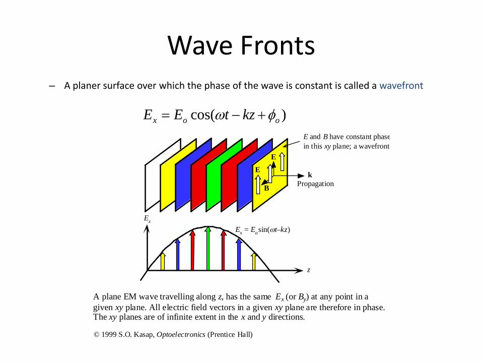
Wave Fronts

)cos( oox kztEE φω +−=

– A planer surface over which the phase of the wave is constant is called a wavefront

z

Ex = Eosin(ωt–kz)Ex

z

Propagation

E

B

k

E and B have constant phasein this xy plane; a wavefront

E

A plane EM wave travelling along z, has the same Ex (or By) at any point in agiven xy plane. All electric field vectors in a given xy plane are therefore in phase.The xy planes are of infinite extent in the x and y directions.

© 1999 S.O. Kasap, Optoelectronics (Prentice Hall)

Optical Field

• Use of E fields to describe light – We know from Electrodynamics that a time varying B field

results in time varying E fields and vise versa – Thus all oscillating E fields have a mutually oscillating B field

perpendicular to both the E field and the direction of propagation

– However, one uses the E field rather than the B field to describe the system

• It is the E field that displaces electrons in molecules and ions in the crystals at optical frequencies and thereby gives rise to the polarization of matter

• Note that the fields are indeed symmetrically linked, but it is the E field that is most often used to characterize the system

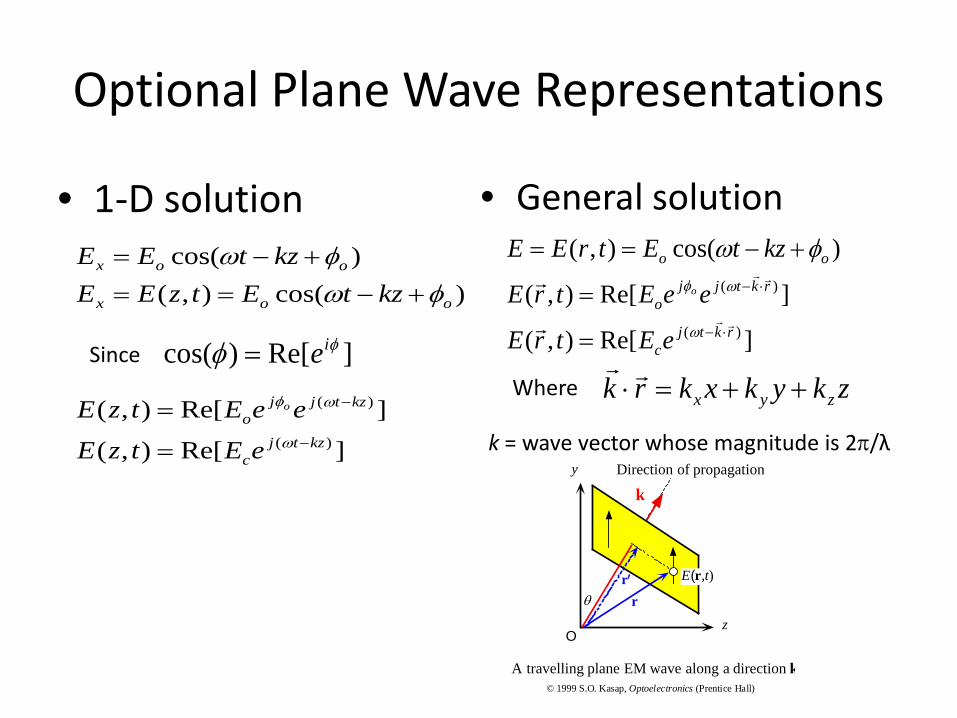
Optional Plane Wave Representations

• 1-D solution

]Re[),(

]Re[),(

)cos(),()cos(

)(

)(

kztjc

kztjjo

oox

oox

eEtzEeeEtzE

kztEtzEEkztEE

o

−

−

=

=

+−==+−=

ω

ωφ

φωφω

]Re[)cos( φφ ie=Since

• General solution

]Re[),(

]Re[),(

)cos(),(

)(

)(

rktjc

rktjjo

oo

eEtrE

eeEtrE

kztEtrEEo

⋅−

⋅−

=

=

+−==

ω

ωφ

φω

zkykxkrk zyx ++=⋅

Where

y

z

kDirection of propagation

r

O

θ

E(r,t)r′

A travelling plane EM wave along a direction k© 1999 S.O. Kasap, Optoelectronics (Prentice Hall)

k = wave vector whose magnitude is 2π/λ

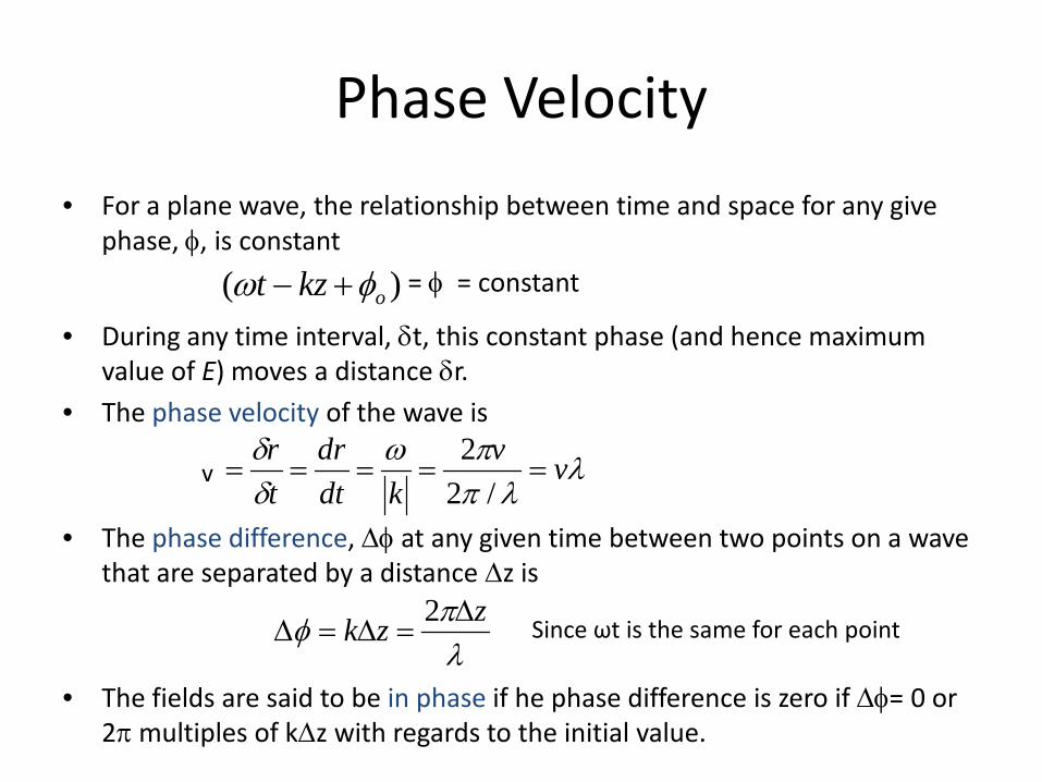
Phase Velocity

• For a plane wave, the relationship between time and space for any give phase, φ, is constant

= φ = constant )( okzt φω +−• During any time interval, δt, this constant phase (and hence maximum

value of E) moves a distance δr. • The phase velocity of the wave is

• The phase difference, ∆φ at any given time between two points on a wave that are separated by a distance ∆z is

• The fields are said to be in phase if he phase difference is zero if ∆φ= 0 or 2π multiples of k∆z with regards to the initial value.

λλπ

πωδδ vv

kdtdr

tr

=====/2

2v

λπφ zzk ∆

=∆=∆2

Since ωt is the same for each point

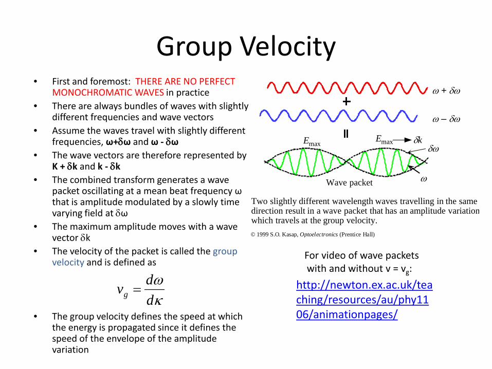
Group Velocity • First and foremost: THERE ARE NO PERFECT

MONOCHROMATIC WAVES in practice • There are always bundles of waves with slightly

different frequencies and wave vectors • Assume the waves travel with slightly different

frequencies, ω+δω and ω - δω • The wave vectors are therefore represented by

K + δk and k - δk • The combined transform generates a wave

packet oscillating at a mean beat frequency ω that is amplitude modulated by a slowly time varying field at δω

• The maximum amplitude moves with a wave vector δk

• The velocity of the packet is called the group velocity and is defined as

• The group velocity defines the speed at which the energy is propagated since it defines the speed of the envelope of the amplitude variation

κω

ddvg =

δω

ω

ω + δω

ω – δω

δkEmax Emax

Wave packet

Two slightly different wavelength waves travelling in the samedirection result in a wave packet that has an amplitude variationwhich travels at the group velocity.© 1999 S.O. Kasap, Optoelectronics (Prentice Hall)

http://newton.ex.ac.uk/teaching/resources/au/phy1106/animationpages/

For video of wave packets with and without v = vg:

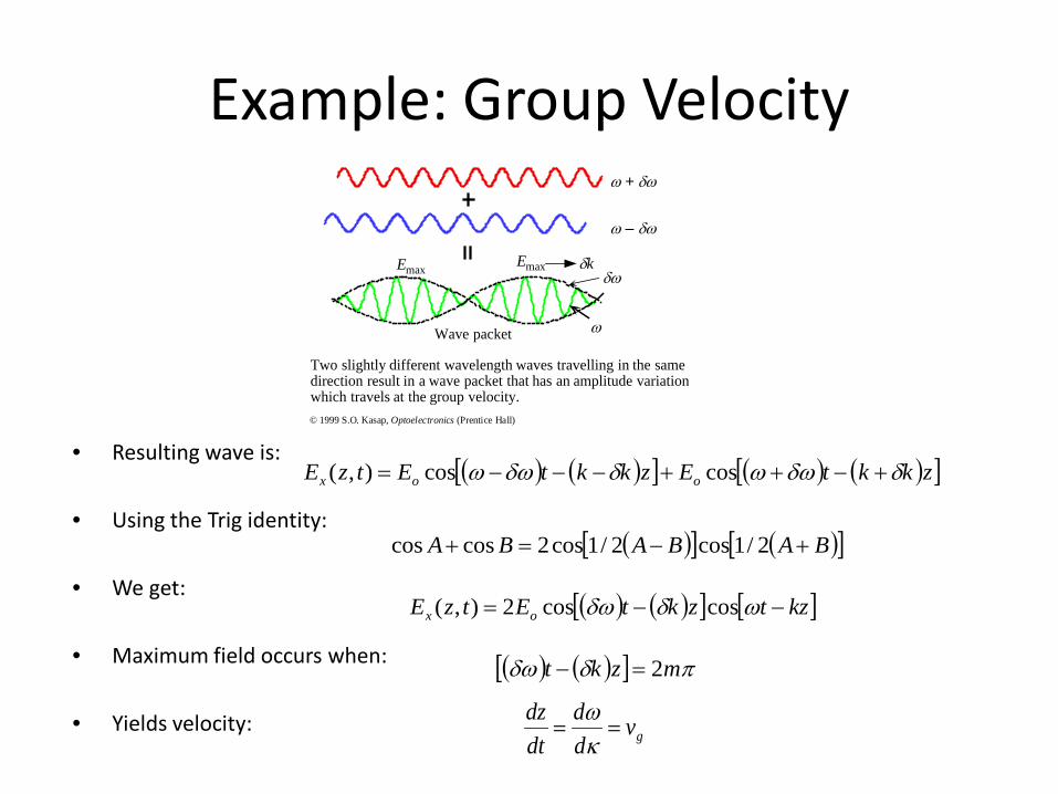
Example: Group Velocity

• Resulting wave is:

• Using the Trig identity:

• We get:

• Maximum field occurs when:

• Yields velocity:

δω

ω

ω + δω

ω – δω

δkEmax Emax

Wave packet

Two slightly different wavelength waves travelling in the samedirection result in a wave packet that has an amplitude variationwhich travels at the group velocity.© 1999 S.O. Kasap, Optoelectronics (Prentice Hall)

( ) ( )[ ] ( ) ( )[ ]zkktEzkktEtzE oox δδωωδδωω +−++−−−= coscos),(

( )[ ] ( )[ ]BABABA +−=+ 2/1cos2/1cos2coscos

( ) ( )[ ] [ ]kztzktEtzE ox −−= ωδδω coscos2),(

( ) ( )[ ] πδδω mzkt 2=−

gvdd

dtdz

==κω

Group Index • Suppose v depends on the λ or K

• By definition, the group velocity is then

• We define Ng as the group index of the medium.

• We now have a way to determine the effect of the medium on the group velocity at different wavelengths (frequency dependence!!!)

• The refractive index, n, and group index, Ng, depend on the permittivity of the material, εr

• We define a dispersive medium is a medium in which both the group and phase velocities depend on the wavelength.

• All materials are said to be dispersive over particular frequency ranges

==

λπω 2

ncvk where n = n(λ)

gg N

c

ddnn

cdkdv =

−==

λλ

ω

Refractive index n and the group index Ng of pureSiO2 (silica) glass as a function of wavelength.

Ng

n

500 700 900 1100 1300 1500 1700 19001.44

1.45

1.46

1.47

1.48

1.49

Wavelength (nm)

© 1999 S.O. Kasap, Optoelectronics (Prentice Hall)

• Ng and n are frequency (wavelength) dependent • Notice the minima for Ng at 1300 nm.

• Ng is wavelength independent near 1300 nm

• Light at 1300 nm travels through SiO2 at the same group velocity without dispersion

Dispersive medium example: SiO2

Example: Effects of a Dispersive Medium

• Consider 1 um wavelength light propagating through SiO2 • At this wavelength, Ng and n are both frequency dependent with no

local minima • Thus the medium is dispersive • Now we must ask the question, are the group and phase velocities of

the propagating wave packet the same?

• Phase Velocity

• Group Velocity

• Answer: NO!!!! The group velocity is 0.9% slower than the phase velocity Refractive index n and the group index Ng of pure

SiO2 (silica) glass as a function of wavelength.

Ng

n

500 700 900 1100 1300 1500 1700 19001.44

1.45

1.46

1.47

1.48

1.49

Wavelength (nm)

© 1999 S.O. Kasap, Optoelectronics (Prentice Hall)

smx

smx

nc

dtdzv 88 10069.2450.1/103 =

===

smx

smx

Nc

dkdv

gg

88 10051.2463.1/103 =

===

ω

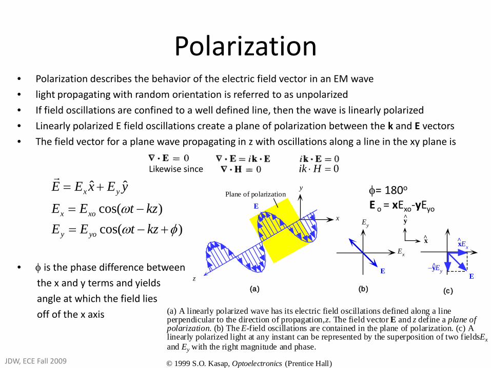
Polarization • Polarization describes the behavior of the electric field vector in an EM wave

• light propagating with random orientation is referred to as unpolarized

• If field oscillations are confined to a well defined line, then the wave is linearly polarized

• Linearly polarized E field oscillations create a plane of polarization between the k and E vectors

• The field vector for a plane wave propagating in z with oscillations along a line in the xy plane is

• φ is the phase difference between

the x and y terms and yields

angle at which the field lies

off of the x axis

x

y

z

Ey

Ex

−yEy^

xEx^

(a) (b) (c )

EPlane of polarization

x

y

E

(a) A linearly polarized wave has its electric field oscillations defined along a lineperpendicular to the direction of propagation, z. The field vector E and z define a plane ofpolarization. (b) The E-field oscillations are contained in the plane of polarization. (c) Alinearly polarized light at any instant can be represented by the superposition of two fields Exand Ey with the right magnitude and phase.

E

© 1999 S.O. Kasap, Optoelectronics (Prentice Hall)

)cos()cos(

ˆˆ

φωω

+−=−=

+=

kztEEkztEE

yExEE

yoy

xox

yx

φ= 180o

E o = xExo-yEyo

JDW, ECE Fall 2009

Likewise since 0=⋅Hik

Circular Polarization • right circular polarization - clockwise rotation of the E field as it propagates along k

• left circular polarization - counter clockwise rotation of the E field as it propagates along k

• Assume that φ = 90o and that the Exo and Eyo fields have the same amplitude. Then

z

Ey

Ex

EEθ = k∆z

∆z

z

A right circularly polarized light. The field vector E is always at rightangles to z , rotates clockwise around z with time, and traces out a fullcircle over one wavelength of distance propagated.

© 1999 S.O. Kasap, Optoelectronics (Prentice Hall)

zkEEE

kztEkztEEkztEE

yExEE

yx

yoyoy

xox

yx

∆=

+=

−−=+−=−=

+=

θ

ωφωω

222

)cos()cos()cos(

ˆˆ

JDW, ECE Fall 2009

Linear and Circular Polarization

E

y

x

Exo = 0Eyo = 1φ = 0

y

x

Exo = 1Eyo = 1φ = 0

y

x

Exo = 1Eyo = 1φ = π/2

E

y

x

Exo = 1Eyo = 1φ = −π/2

(a) (b) (c) (d)

Examples of linearly, (a) and (b), and circularly polarized light (c) and (d); (c) isright circularly and (d) is left circularly polarized light (as seen when the wavedirectly approaches a viewer)

© 1999 S.O. Kasap, Optoelectronics (Prentice Hall)

JDW, ECE Fall 2009

Linear and Elliptical Polarization

• Assume that the magnitude of one vector component in E is larger then the other

• Instead of a circle, the wave generates and ellipse as it propagates along k in the z direction

E

y

x

Exo = 1Eyo = 2φ = 0

Exo = 1Eyo = 2φ = π/4

Exo = 1Eyo = 2φ = π/2

y

x

(a) (b)E

y

x

(c)

(a) Linearly polarized light with Eyo = 2Exo and φ = 0. (b) When φ = π/4 (45°), the light isright elliptically polarized with a tilted major axis. (c) When φ = π/2 (90°), the light isright elliptically polarized. If Exo and Eyo were equal, this would be right circularlypolarized light.

© 1999 S.O. Kasap, Optoelectronics (Prentice Hall)

JDW, ECE Fall 2009

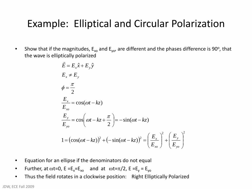
Example: Elliptical and Circular Polarization

• Show that if the magnitudes, Exo and Eyo, are different and the phases difference is 90o, that the wave is elliptically polarized

• Equation for an ellipse if the denominators do not equal

• Further, at ωt=0, E =Ex=Exo and at ωt=π/2, E =Ey = Eyo

• Thus the field rotates in a clockwise position: Right Elliptically Polarized

( ) ( )22

22 )sin()cos(1

)sin(2

cos

)cos(

2

ˆˆ

+

=−−+−=

−−=

+−=

−=

=

≠

+=

yo

y

xo

x

yo

y

xo

x

yx

yx

EE

EEkztkzt

kztkztEE

kztEE

EEyExEE

ωω

ωπω

ω

πφ

JDW, ECE Fall 2009

Energy Flow in EM Waves

• Let us recall that there is indeed a B field in the EM wave.

• Recall from electrostatics that

• where

• As the EM wave propagates along the direction k, there is an energy flow in that direction

– Electrostatic energy density

– Magnetostatic energy density

• The Energy flow per unit time per unit area, S, is defined as the Poynting Vector

( )r

oor

yyx

n

v

BncvBE

ε

µεε

=

=

==

−1

22

2

221

21

yo

yo

xor

HB

E

µµ

εε

=

Where both these values are equal

( )( ) ( )

HEHEcn

ncHEvBEvS

BEvEvtA

EtAvHES

ooror

yxorxorxor

oo

×=×=×=×=

==∆

∆=×=

2

2

2

222

222

µεεεε

εεεεεε

Speed of light in the medium

Irradiance • Magnitude of the Pointing Vector is called the irradiance

• Note that because we are discussing sinusoidal waveforms, that the instantaneous irradiance of light propagating in phase is taken from the instantaneous amplitude of E and B respectively

• Instantaneous irradiance can only be measured if the power meter responds more quickly than the electric field oscillations.

• As one might imagine, at optical frequencies, all practice measurements are made using the average irradiance.

• The average irradiance is

yxor BEvS εε2=

HEHEcn

ncHE

nc

HEvBEv

nEsmEcnE

nc

EvSSI

oor

oorooor

ooooor

ooravg

×=×=×=

×==

×===

===

21

21

21

21

21

1033.121

21

21

2

22

2

2

2

22

2822

2

µεε

µεεεε

εεε

εε

Radiation from a Point Source

• Radiation from a point source such as an atom requires a slightly more complicated solution than that of a plane wave.

• Such sources are analyzed in term of the vector potential, A, and the scalar potential φ

• The potential for the atom must be an oscillating function to generate a light wave

• Where ρ is the charge density and the potential falls off as 1/r such that the radial field emanating from the atom falls off as 1/r2

• For distances far from the source it is conventional to expand the potential in terms of r powers of the form k1r+k2r3. Where the quadruple terms is orders of magnitude smaller than the dipole term, and so on and so on.

8/20/2012 33

• Apply Maxwell’s equations to dielectric materials

• Assume that the magnetization, M, and the ρ are both zero

• And again if we take the curl of equation 4 and the time derivative of equation 3, one can eliminate H to get:

• The first source term describes the polarization charges within the dielectric

• The second term describes conduction charges that are applicable to metallic materials

Maxwell’s Time Dependent Equations in a Medium

Differential Form

tBE

JtDH

BD v

∂∂

−=×∇

+∂∂

=×∇

=⋅∇

=⋅∇

0ρ

Recalling:

8/20/2012 34

• Lasers gain materials are typically comprised of dielectrics that do not conduct.

• Thus we are concerned primarily about the effects of polarization and less on electric conduction, let us ignore the conduction term and assume the source term to be soley due to polarization of the medium by the electric field.

• Let us assume therefore that the gain media we will use has a macroscopic polarization that can be characterized using the following equation:

• Where x is a vector representing the distance that the charge of the electron is displaced from its equilibrium position, N is the number of changes, and e is the unit of charge

• The term is known as the electric dipole.

Maxwell’s Time Dependent Equations in a Medium

8/20/2012 35

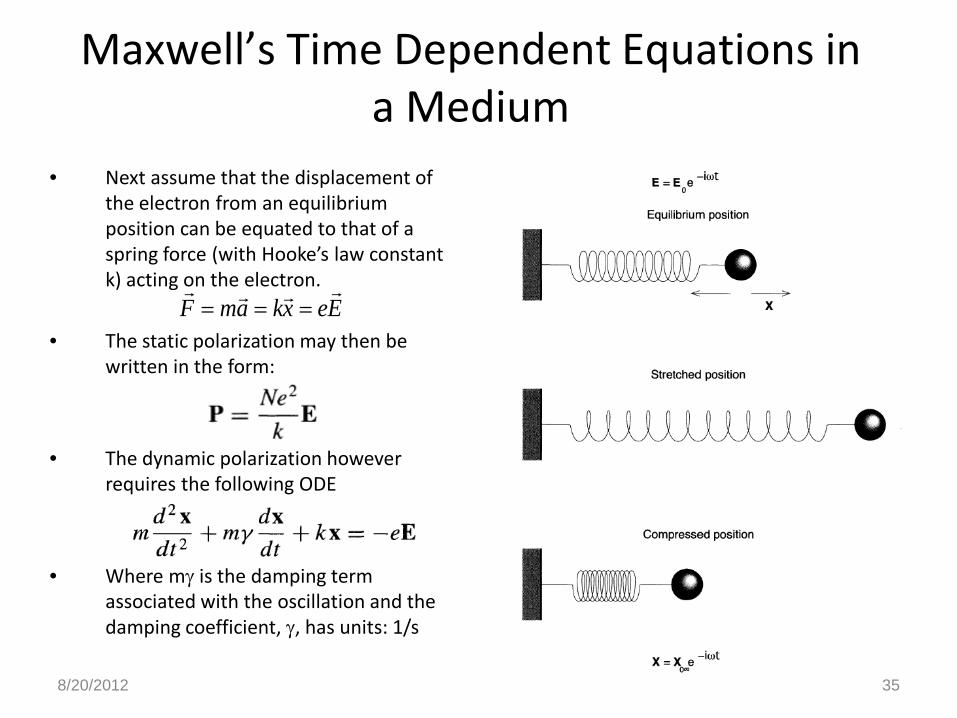
• Next assume that the displacement of the electron from an equilibrium position can be equated to that of a spring force (with Hooke’s law constant k) acting on the electron.

• The static polarization may then be written in the form:

• The dynamic polarization however requires the following ODE

• Where mγ is the damping term associated with the oscillation and the damping coefficient, γ, has units: 1/s

Maxwell’s Time Dependent Equations in a Medium

EexkamF

===

8/20/2012 36

• Given a time harmonic e field, with angular frequency, ω

• The following 2nd order ODE can be reduced to the following equation:

• Using this equation to solve for x and substituting for the polarization value required for the static condition, one receives

• Which reduces to the static value when ω = 0

• The frequency dependent value also demonstrates a resonant frequency at

• Which allows the more conventional form of the expression:

Maxwell’s Time Dependent Equations in a Medium

8/20/2012 37

• Let’s now take this further and plug our value for P back into our Curl equation for E

• For a medium in which there is no local charge density, Gauss’s law requires

• This can also be used to show that

• Then using the math identity (coupled with the physical divergence condition above)

• One can write:

• Where

Maxwell’s Time Dependent Equations in a Medium

8/20/2012 38

• The term Kz presented is obviously a complex number that we can separate into both real and complex parts

• Allowing one to separate the propagating and damping components of the electric field as

• Where αE is the extinction index representing the exponential decay of the electric field as it travels a distance z into the medium

• As we discussed before, the energy associated with the field is proportional to the square of said field. Thus, the exponential decay of energy in the field is proportional to

and we can define a new term α as the asorption coefficient which has units of 1/m and determines the amount of energy absorbed over distance traveled. The absorption depth we define as ld=1/α

Maxwell’s Time Dependent Equations in a Medium

8/20/2012 39

• The use of the complex coefficient Kz is equivalent to the complex index of refraction

Maxwell’s Time Dependent Equations in a Medium

8/20/2012 40

• So how does one use the relation for N2 to obtain the values for the real and imaginary refractive index

• One can start by evaluating the real and imaginary terms associated with N2 as:

• At the resonance frequency, these terms reduce to the following simple solution

Maxwell’s Time Dependent Equations in a Medium

+ terms lead to positive refractive indices, - terms lead to negative refractive indices

Idealized Dispersion Curve

• Real materials have multiple electron states with multiple time constants responding to a series of natural frequencies associated with different electron orbitals in the molecular media

• Absorption in regions not near resonance also has a significant frequency dependence which is partially due to ω but more and more due to the imaginary component of the index as the wavelength approaches the X-ray region

• If within a given frequency range, γ is small, then it can sometimes be neglected yielding Sellmeier’s Formula:

Dispersion Curve for a Real Material

Transmission vs. wavelength example for undoped lithium tantalate

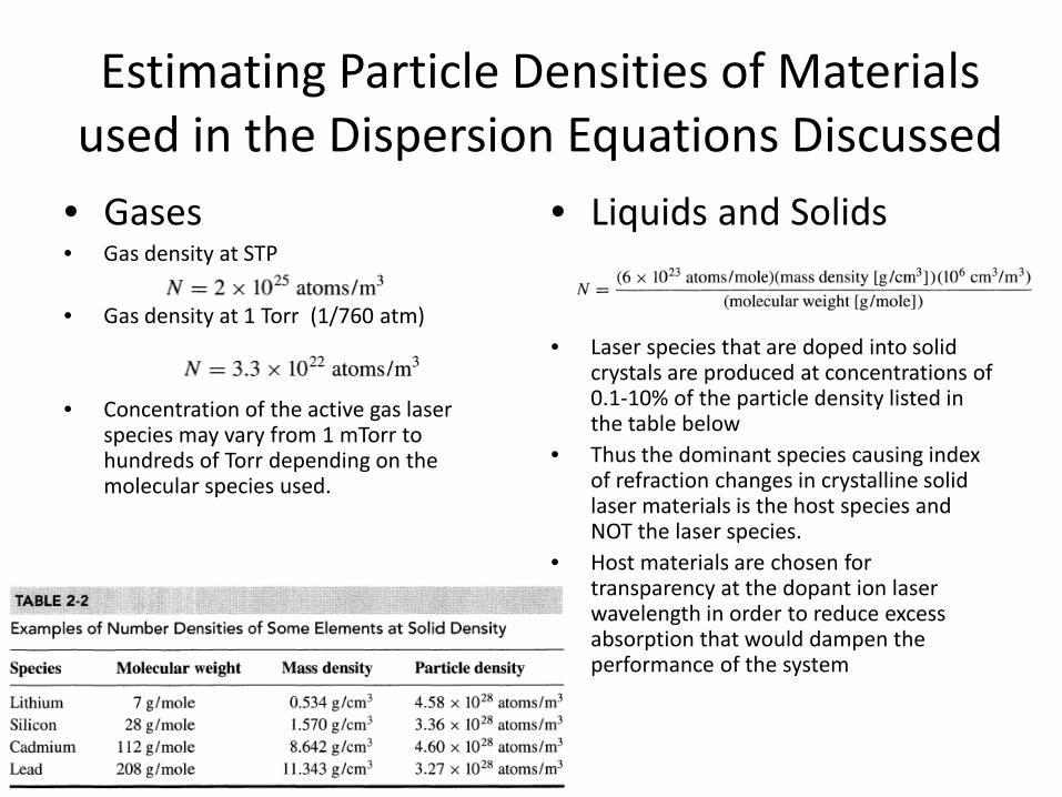
Estimating Particle Densities of Materials used in the Dispersion Equations Discussed

• Gases • Gas density at STP

• Gas density at 1 Torr (1/760 atm)

• Concentration of the active gas laser species may vary from 1 mTorr to hundreds of Torr depending on the molecular species used.

• Liquids and Solids

• Laser species that are doped into solid crystals are produced at concentrations of 0.1-10% of the particle density listed in the table below

• Thus the dominant species causing index of refraction changes in crystalline solid laser materials is the host species and NOT the laser species.

• Host materials are chosen for transparency at the dopant ion laser wavelength in order to reduce excess absorption that would dampen the performance of the system

Coherence • Let us assume for a second that we manage to create a laser. Second, let us assume

(correctly) that we have not matched every mode solution in the system perfectly

• The laser will operate at wavelengths that may be very slightly different

• OR we might use two different lasers with slightly different operational wavelengths

• In such cases, the two distinct waves will interfere to produce dramatic effects.

• Such effects, include longitudinal modes, mode-locking, frequency multiplication, and phase matching. These will all be discussed in detail in future chapters

• Let us first however introduce the basic concepts of two separate waves interacting with one another

• The resulting intensity is:

• If k1 and k2 and ω1 and ω2 are similar then the two waves are said to be coherent

• If the k vectors are drastically different or originate at very different locations then the waves do not interfere and are said to be incoherent

Coherence • Mathematical statement for coherence:

• Partial coherence occurs when interference still exists, but complete coherence is not achieved

• Coherence is said to be either temporal or spatial

• Temporal coherence (longitudinal coherence): two waves at different frequencies

Temporal Coherence Example

Note: This example is asking you to find the temporal coherence length for each of the two independent systems

Coherence

• Spatial coherence (transverse coherence): two waves at the same frequency but peaking at different points in space

Optional slides following

8/20/2012 50

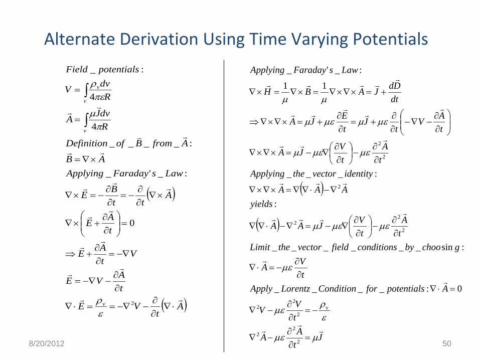
Alternate Derivation Using Time Varying Potentials

( )

( )

JtAA

tVV

ApotentialsforConditionLorentzApplytVA

gchoobyconditionsfieldvectortheLimittA

tVJAA

yieldsAAA

identityvectortheApplyingtA

tVJA

tAV

tJ

tEJA

dtDdJABH

LawsFaradayApplying

v

µµε

ερµε

µε

µεµεµ

µεµεµ

µεµµεµ

µµ

=∂∂

−∇

−=∂∂

−∇

=⋅∇∂∂

−=⋅∇

∂∂

−

∂∂

∇−=∇−⋅∇∇

∇−⋅∇∇=×∇×∇

∂∂

−

∂∂

∇−=×∇×∇

∂∂

−∇−∂∂

+=∂∂

+=×∇×∇⇒

+=×∇×∇=×∇=×∇

2

22

2

22

2

22

2

2

2

0:____

:sin______

:

:___

11

:_'_

( )

( )At

VE

tAVE

VtAE

tAE

Att

BE

LawsFaradayApplyingAB

AfromBofDefinition

RdvJA

RdvV

potentialsField

v

v

v

v

⋅∇∂∂

−−∇==⋅∇

∂∂

−−∇=

−∇=∂∂

+⇒

=

∂∂

+×∇

×∇∂∂

−=∂∂

−=×∇

×∇=

=

=

∫

∫

2

0

:_'_

:____

4

4

:_

ερ

πµ

περ

8/20/2012 51

Wave Equation

00

00

2

22

2

22

2

22

2

22

1

1

___

εµµε

εµ

µε

µε

µε

µµε

ερµε

==

=

=

∂∂

=∇

∂∂

=∇

=∂∂

−∇

−=∂∂

−∇

ucn

c

u

tBB

tEE

yieldsspacefreeIn

JtAA

tVV v

Refractive index

Speed of the wave in a medium

Speed of light in a vacuum