Laser Beams and Resonators - physics.byu.edu beams and resonators, ... this will be discussed in...

Laser Beams and Resonators

H. KOGELNIK AND T. LI

Abstract-This paper is a review of the theory-of laser beams andresonators. It is meant to be tutorial in nature and useful in scope. Noattempt is made to be exhaustive in the treatment. Rather, emphasis isplaced on formulations and derivations which lead to basic understand-ing and on results which bear practical significance.

1. INTRODUCTION

rT HE COHERENT radiation generated by lasers ormasers operating in the optical or infrared wave-length regions usually appears as a beam whose

transverse extent is large compared to the wavelength.The resonant properties of such a beam in the resonatorstructure, its propagation characteristics i free space, andits interaction behavior with various optical elements anddevices have been studied extensively in recent years.This paper is a review of the theory of laser beams andresonators. Emphasis is placed on formulations andderivations which lead to basic understanding and onresults which are of practical value.

Historically, the subject of laser resonators had itsorigin when Dicke [1], Prokhorov [2], and Schawlow andTownes [3] independently proposed to use the Fabry-Perot interferometer as a laser resonator. The modes insuch a structure, as determined by diffraction effects,were first calculated by Fox and Li [4]. Boyd and Gordon[5], and Boyd and Kogelnik [6] developed a theory forresonators with spherical mirrors and approximated themodes by wave beams. The concept of electromagneticwave beams was also introduced by Goubau and Schwe-ring [7], who investigated the properties of sequences oflenses for the guided transmission of electromagneticwaves. Another treatment of wave beams was given byPierce [8]. The behavior of Gaussian laser beams as theyinteract with various optical structures has been analyzedby Goubau [9], Kogelnik [10], [11], and others.

.9The present paper summarizes the various thebries andis divided into three parts. The first part treats the passageof paraxial rays through optical structures and is basedon geometrical optics. The second part is an analysis oflaser beams and resonators, taking into account the wavenature of the beams but ignoring diffraction effects dueto the finite size of the apertures. The third part treats theresonator modes, taking into account aperture diffrac-tion effects. Whenever applicable, useful results are pre-sented in the forms off formulas, tables, charts, andgraphs.

Manuscript received July 12, 1966.H. Kogelnik is with Bell Telephone Laboratories, Inc., Murray

Hill, N. JiT. Li is with Bell Telephone Laboratories, Inc., Holmdel, N. J.

2. PARAXIAL RAY ANALYSIS

A study of the passage of paraxial rays through opticalresonators, transmission lines, and similar structures canreveal many important properties of these systems. Onesuch "geometrical" property is the stability of the struc-ture [6], another is the loss of unstable resonators [12].The propagation of paraxial rays through various opticalstructures can be described by ray transfer matrices.Knowledge of these matrices is particularly useful as theyalso describe the propagation of Gaussian beams throughthese structures; this will be discussed in Section 3. Thepresent section describes briefly some ray concepts whichare useful in understanding laser beams and resonators,and lists the ray matrices of several optical systems ofinterest. A more detailed treatment of ray propagationcan be found in textbooks [13] and in the literature onlaser resonators [14].

I I

XI,,, I __ P!!tht - - -"~ _

I I

I P R NACI PA L _ _e lPLANES

INPUT OUTPUTPLANE PLANE

Fig. 1. Reference planes of an optical system.A typical ray path is indicated.

2.1 Ray Transfer Matrix

A paraxial ray in a given cross section (z=const) of anoptical system is characterized by its distance x from theoptic (z) axis and by its angle or slope x' with respect tothat axis. A typical ray path through an optical structureis shown in Fig. 1. The slope x' of paraxial rays is assumedto be small. The ray path through a given structure de-pends on the optical properties of the structure and on theinput conditions, i.e., the position x and the slope x' ofthe ray in the input plane of the system. For paraxial raysthe corresponding output quantities x2 and x2' are linearlydependent on the input quantities. This is convenientlywritten in the matrix form

X9 -A B xi

X2i C D xi' (1)

1550 APPLIED OPTICS / Vol. 5, No. 10 / October 1966

:

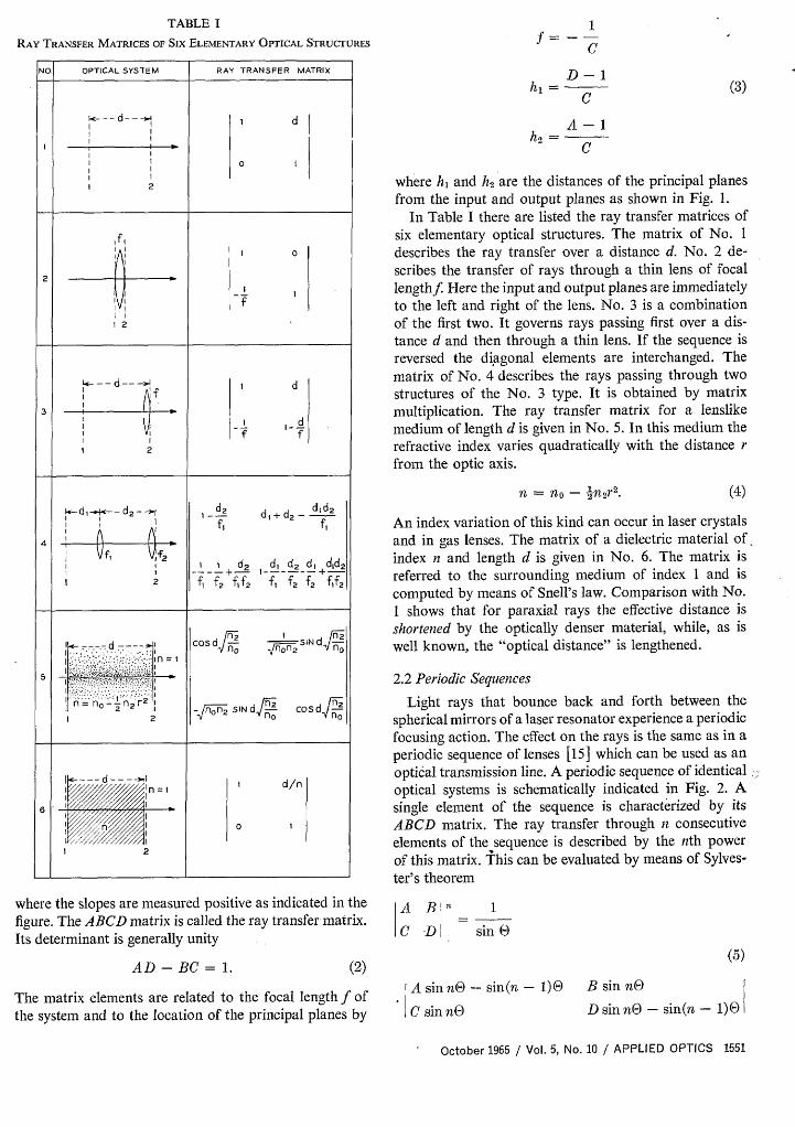
TABLE I

RAY TRANSFER MATRICES OF Six ELEMENTARY OPrICAL STRUCTURES f CC

NO. OPTICAL SYSTEM RAY TRANSFER MATRIX D= (3)

C

1 A-i

where hi and h2 are the distances of the principal planesfrom the input and output planes as shown in Fig. 1.

In Table I there are listed the ray transfer matrices ofsix elementary optical structures. The matrix of No. I

IIj a O describes the ray transfer over a distance d. No. 2 de-

2 [ 8 W scribes the transfer of rays through a thin lens of focal1 ' l lengthf Here the input and output planes are immediately

l l f to the left and right of the lens. No. 3 is a combination1 2 of the first two. It governs rays passing first over a dis-

tance d and then through a thin lens. If the sequence isreversed the diagonal elements are interchanged. The

d - d matrix of No. 4 describes the rays passing through twof l structures of the No. 3 type. It is obtained by matrix

-! _ A multiplication. The ray transfer matrix for a lenslikel Id medium of length d is given in No. 5. In this medium the1 2 refractive index varies quadratically with the distance r

from the optic axis.

d~~~~~~~~d2~ ~ ~ ~ ~ ~ n = no - n2r . (4)

Id A d + 1 f2 d dI _ ftf 2 An index variation of this kind can occur in laser crystals

4 and in gas lenses. The matrix of a dielectric material of

lf d2 d, d2 d, dd2 index n and length d is given in No. 6. The matrix is2¶fl f2 ff2 fl f2 f2 ff2 referred to the surrounding medium of index 1 and is

computed by means of Snell's law. Comparison with No.1 shows that for paraxial rays the effective distance is

FI12 shortened by the optically denser material, while, as isa - -d- - > S cosdn - nSI nd - well known, the "optical distance" is lengthened.

l no: ..::: no.;, :i n I5 l : S t;. S S ifl.

5 K 2.2 Periodic Sequences

n n0o 2 n2 r2

i n Nd cosd Light rays that bounce back and forth between the2 no no spherical mirrors of a laser resonator experience a periodic

focusing action. The effect on the rays is the same as in aperiodic sequence of lenses [15] which can be used as anoptical transmission line. A periodic sequence of identical

n -Id/n optical systems is schematically indicated in Fig. 2. A

6- '_ XX/X/5X////@single element of the sequence is characterized by itso / ABCD matrix. The ray transfer through n consecutive

elements of the sequence is described by the nth power2

of this matrix. This can be evaluated by means of Sylves-ter's theorem

where the slopes are measured positive as indicated in the A B n 1figure. The ABCD matrix is called the ray transfer matrix.Its determinant is generally unity C D sin 0

AD-BC = 1. (2) (5)

The matrix elements are related to the focal length f of A sin n@ - sin(n - 1)0 B sin nIthe system and to the location of the principal planes by C sin nO D sin nO - sin(n - 1)0

October 1966 / Vol. 5, No. 10 / APPLIED OPTICS 1551

cos ) = (A + D).

Periodic sequences can be classified as either stable orunstable. Sequences are stable when the trace (A+D)obeys the inequality

-1 < (A2 + D) < 1. (7)

Inspection of (5) shows that rays passing through a stablesequence are periodically refocused. For unstable sys-tems, the trigonometric functions in that equation be-come hyperbolic functions, which indicates that the raysbecome more and more dispersed the further they passthrough the sequence. R = 2f, , R = 2f2

Fig. 3. Spherical-mirror resonator and theequivalent sequence of lenses.

( ) Xl') Xn

Fig. 2. Periodic sequence of identical systems,each characterized by its ABCD matrix.

2.3 Stability of Laser ResonatorsA laser resonator with spherical mirrors of unequal

curvature is a typical example of a periodic sequence thatcan be either stable or unstable [6]. In Fig. 3 such aresonator is shown together with its dual, which is asequence of lenses. The ray paths through the two struc-tures are the same, except that the ray pattern is folded inthe resonator and unfolded in the lens sequence. The focallengths j; and f of the lenses are the same as the focallengths of the mirrors, i.e., they are determined by theradii of curvature R and R2 of the mirrors (fi=R,/2,f 2 =R 2/2). The lens spacings are the same as the mirrorspacing d. One can choose, as an element of the peri-odic sequence, a spacing followed by one lens plus anotherspacing followed by the second lens. The ABCD matrixof such an element is given in No. 4 of Table I. From thisone can obtain the trace, and write the stability condition(7) in the form

0 < (I ) (1-) < 1. (8)

To show graphically which type of resonator is stableand which is unstable, it is useful to plot a stability dia-gram on which each resonator type is represented by apoint. This is shown in Fig. 4 where the parameters d/R,and d/R 2 are drawn as the coordinate axes; unstablesystems are represented by points in the shaded areas.Various resonator types, as characterized by the relativepositions of the centers of curvature of the mirrors, areindicated in the appropriate regions of the diagram. Alsoentered as alternate coordinate axes are the parameters g1and 2 which play an important role in the diffractiontheory of resonators (see Section 4).

'7 /~~~~~~~

A g I ONP C--

:( ICONFOCAL-

I (RI= R 2 = d)

/ CONCENTRICX(R = R2 = d/2)

</WI

ARA LL L

_N 42 - -PLAEI

0 1 - < -

0~~~~~~~ I =I -

-1

Fig. 4. Stability diagram. Unstable resonatorsystems lie in shaded regions.

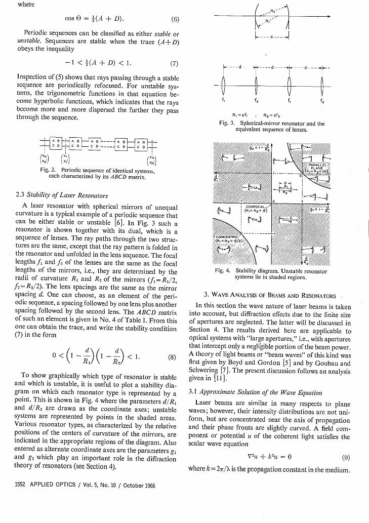
3. WAVE ANALYSIS OF BEAMS AND RESONATORS

In this section the wave nature of laser beams is takeninto account, but diffraction effects due to the finite sizeof apertures are neglected. The latter will be discussed inSection 4. The results derived here are applicable tooptical systems with "large apertures," i.e., with aperturesthat intercept only a negligible portion of the beam power.A theory of light beams or "beam waves" of this kind wasfirst given by Boyd and Gordon [5] and by Goubau andSchwering [7]. The present discussion follows an analysisgiven in [11].

3.1 Approximate Solution of the Wave Equation

Laser beams are similar in many respects to planewaves; however, their intensity distributions are not uni-form, but are concentrated near the axis of propagationand their phase fronts are slightly curved. A field com-ponent or potential of the coherent light satisfies thescalar wave equation

V2 u + k2u = 0 (9)

where k = 27r/X is the propagation constant in the medium.


where

(6)

--- d---;

d- -- ---d--- II --- ---- A

f, fz f, f2

l t o i Z z w w w w r w w Z P w P - -

For light traveling in the z direction one writes t E

iu = V,(x, y, z) exp(-jkz) (10)

where 4' is a slowly varying complex function whichrepresents the differences between a laser beam and aplane wave, namely: a nonuniform intensity distribu-tion, expansion of the beam with distance of propagation,curvature of the phase front, and other differences dis-cussed below. By inserting (10) into (9) one obtains

+ - 2jk - = ° (11)Ox2 ay2 OZ

where it has been assumed that 4' varies so slowly with zthat its second derivative 024'/0z2 can be neglected.

The differential equation (11) for A/ has a form similarto the time dependent Schrddinger equation. It is easy tosee that

4 exp {- + 2 r2 (12)

is a solution of (11), where

r2 = 2 + y2 . (13)

The parameter P(z) represents a complex phase shift whichis associated with the propagation of the light beam, andq(z) is a complex beam parameter which describes theGaussian variation in beam intensity with the distance rfrom the optic axis, as well as the curvature of the phasefront which is spherical near the axis. After insertion of(12) into (11) and comparing terms of equal powers in rone obtains the relations

q = I (14)

r,,

Go

Fig. 5. Amplitude distribution of the fundamental beam.

When (17) is inserted in (12) the physical meaning of thesetwo parameters becomes clear. One sees that R(z) is theradius of curvature of the wavefront that intersects theaxis at z, and w(z) is a measure of the decrease of thefield amplitude E with the distance from the axis. Thisdecrease is Gaussian in form, as indicated in Fig. 5, andw is the distance at which the amplitude is l/e times thaton the axis. Note that the intensity distribution is Gaus-sian in every beam cross section, and that the width ofthat Gaussian intensity profile changes along the axis.The parameter w is often called the beam radius or "spotsize," and 2w, the beam diameter.

The Gaussian beam contracts to a minimum diameter2wo at the beam waist where the phase front is plane. Ifone measures z from this waist, the expansion laws forthe beam assume a simple form. The complex beamparameter at the waist is purely imaginary

-rI f2

qo = (18)

and a distance z away from the waist the parameter is

7rwo2

q = q + = j + .

(15)P = -

q

where the prime indicates differentiation with respect to z.The integration of (14) yields

After combining (19) and (17) one equates the real andimaginary parts to obtain

W(Z) = W2 1 + (-2) ]q2 = q1 + Z

(20)

(16)

which relates the beam parameter q2 in one plane (outputplane) to the parameter q, in a second plane (input plane)separated from the first by a distance z.

3.2 Propagation Laws for the Fundamental Mode

A coherent light beam with a Gaussian intensity pro-file as obtained above is not the only solution of (11),but is perhaps the most important one. This beam is oftencalled the "fundamental mode" as compared to the higherorder modes to be discussed later. Because of its impor-tance it is discussed here in greater detail.

For convenience one introduces two real beam param-eters R and w related to the complex parameter q by

and

R(Z) = Z[ ( . (21)

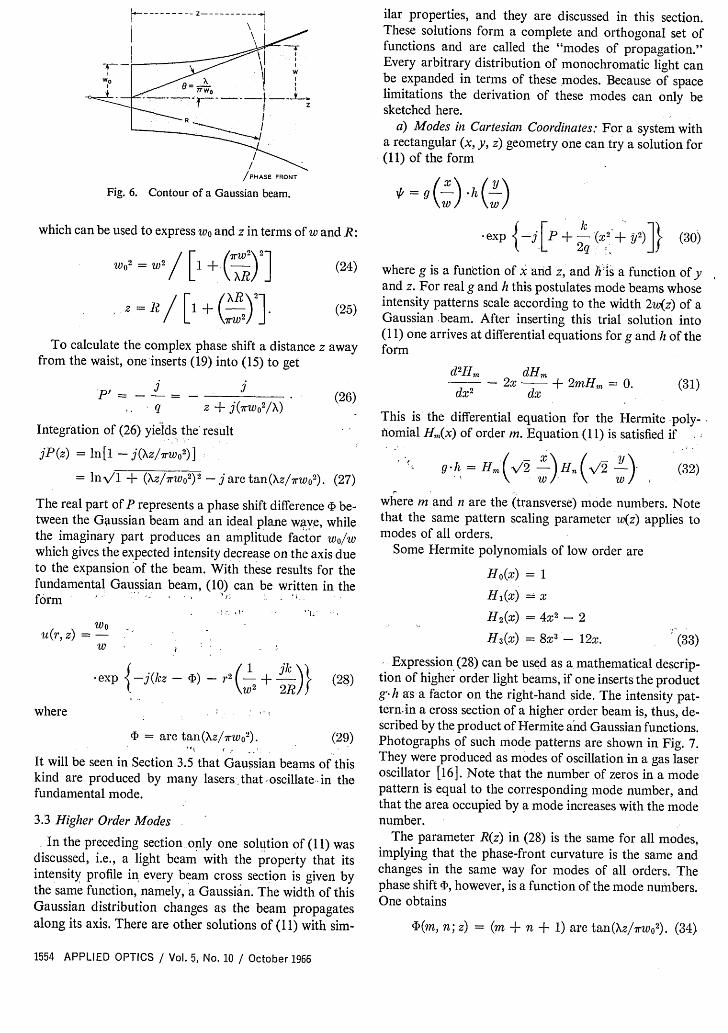
Figure 6 shows the expansion of the beam according to(20). The beam contour w(z) is a hyperbola with asymp-totes inclined to the axis at an angle

(22)0=-*7rWo

This is the far-field diffraction angle of the fundamentalmode.

Dividing (21) by (20), one obtains the useful relation

1 1 *X- - .q R 7rW

2


and (19)

(17)Xz rWI2

rwo2 AR(23)

ilar properties, and they are discussed in this section.These solutions form a complete and orthogonal set offunctions and are called the "modes of propagation."Every arbitrary distribution of monochromatic light canbe expanded in terms of these modes. Because of spacelimitations the derivation of these modes can only besketched here.

a) Modes in Cartesian Coordinates: For a system witha rectangular (x, y, z) geometry one can try a solution for(11) of the form

g h

which can be used to express w0 and z in terms of w and R:

wo2 = W2j [1 + (-) (24)

/ = R 1 (R) 2 ] (25)To calculate the complex phase shift a distance z away

from the waist, one inserts (1-9) into (15) to get

I j1p, (26)q z + j(rwo 2 /X)

Integration of (26) yields the result

jP(z) = ln [1 - j(Xz/7rwo2)]

= ln-\/l + (z/7rw2)2 - j arc tan(Xz/rwO2 ). (27)

The real part of P represents a phase shift difference cJ be-tween the Gaussian beam and an ideal plane wave, whilethe imaginary part produces an amplitude factor w/wwhich gives the expected intensity decrease on the axis dueto the expansion of the beam. With these results for thefundamental Gaussian beam, (10) can be written in theform '

; ts "1 -\,*

wOit(r, z) =-

w

exp {-j(kz - ) -r2( - + R)} (28)

where

D= arc tan(XZ/7rWO2). (29)

It will be seen in Section 3.5 that Gaussian beams of thiskind are produced by many lasers, that oscillate in thefundamental mode.

3.3 Higher Order Modes

In the preceding section only one solution of ( 1) wasdiscussed, i.e., a light beam with the property that itsintensity profile in every beam cross section is given bythe same function, namely, a Gaussian. The width of thisGaussian distribution changes as the beam propagatesalong its axis. There are other solutions of (11) with sim-

{ F [ 2q , ]}, e -j P + -'(XI 2. 2q j). (30)

where g is a function of x and z, and h is a function of yand z. For real g and h this postulates mode beams whoseintensity patterns scale according to the width 2w(z) of aGaussian beam. After inserting this trial solution into(11) one arrives at differential equations for g and h of theform

d2 Hm dHrndx2 - 2x x + 2mHm = 0. (31)

> dx2 ~~~dxThis is the differential equation for the Hermite poly-ftomial Hm(x) of order m. Equation (11) is satisfied if

.g J = Hm./2 -)H (,/2 &) (32),~~~~ W

where m and n are the (transverse) mode numbers. Notethat the same pattern scaling parameter w(z) applies tomodes of all orders.

Some Hermite polynomials of low order are

Ho(x) = 1Hl(x) = xH 2(x) = 4X2 - 2

H3(x) = 8x 3- 12x. (33)

Expression (28) can be used as a mathematical descrip-tion of higher order light beams, if one inserts the productg' h as a factor on the right-hand side. The intensity pat-ternin a cross section of a higher order beam is, thus, de-scribed by the product of Hermite and Gaussian functions.Photographs of such mode patterns are shown in Fig. 7.They were produced as modes of oscillation in a gas laseroscillator [16]. Note that the number of zeros in a modepattern is equal to the corresponding mode number, andthat the area occupied by a mode increases with the modenumber.

The parameter R(z) in (28) is the same for all modes,implying that the phase-front curvature is the same andchanges in the same way for modes of all orders. Thephase shift 4, however, is a function of the mode numbers.One obtains

4(m, n; z) = (m + n + 1) arc tan(Xz/7rwo2). (34)


/ F/ PHASE FRONT

Fig. 6. Contour of a Gaussian beam.

i

________

___

__________

TEt9140

___EN_____

TEIM go

TEIMt a

TEME l

IEM21 , tM 2 2 I tM 3 3

Fig. *4 Mode patterns of a gas laser oscil-lator (rectangular symmetry).

This means that the phase velocity increases with increas-ing mode number. In resonators this leads to differencesin the resonant frequencies of the various modes of oscil-lation.

b) Modes in Cylindrical Coordinates: For a system witha cylindrical (r, , z) geometry one uses a trial solutionfor (11) of the form

(w = exp ! (a + -rol+ )4 ' = 0I }t q (35)

After some calculation one finds=(v Lj\/2. Lp'(2 5) c(36)where Lp4 i a generalized Laguerre polynomial, and pand I are the radial and angular mode numbers. L,'(x)obeys the differential equation

X 2 +(l +1-x) + p 'l= 0. (37)dxl dx

Some polynomials of low order are

Lo'(x) = 1

Lll(x) = + 1-x

L 21(x) = 2'(l + 1) (I + 2) - (I + 2)x + x2. (38)

As in the case of beams with a rectangular geometry, thebeam parameters w(z) and R(z) are the same for all cylin-drical modes. The phase shift is, again, dependent on themode numbers and is given by

43(p, ; z) = (2p + + 1) arc tan(Xz/rwo 2 ). (39)

3.4 Beam Transformation by a Lens

A lens can be used to focus a laser beam to a small spot,or to produce a beam of suitable diameter and phase-front curvature for injection into a given optical structure.An ideal lens leaves the transverse field distribution of abeam mode unchanged. i.e., an incoming fundamentalGaussian beam will emerge from the lens as a funda-mental beam, and a higher order mode remains a modeof the same order after passing through the lens. However,a lens does change the beam parameters R(z) and w(z).As these two parameters are the same for modes of allorders, the following discussion is valid for all orders;the relationship between the parameters of an incomingbeam (labeled here with the index 1) and the parametersof the corresponding outgoing beam (index 2) is studied indetail.

An ideal thin lens of focal lengthf transforms an incom-ing spherical wave with a radius R1 immediately to theleft of the lens into a spherical wave with the radius R 2

immediately to the right of it, where

1 1 1

t2 f 1 f(40)

Figure 8 illustrates this situation. The radius of curvatureis taken to be positive if the wavefront is convex asviewed from z= -oc. The lens transforms the phase frontsof laser beiafrs in eactly the same way as those of sphericalwaves. As the diameter of a beam is the same immediatelyto the left and to the right of a thin lens, the q-parametersof the incoming and outgoing beams are related by

1 1 1

q2 qi f(41)

where the q's are measured at the lens. If q, and q2 aremeasured at distances d1 and d2 from the lens as indicatedin Fig. 9, the relation between them becomes

q2 =(1 - d2/f)qi + (d, + d2 - did2/f)

-(il'f) + ( -df)(42)

This formula is derived using (16) and (41).More complicated optical structures, such as gas lenses,

combinations of lenses, or thick lenses, can be thought ofas composed of a series of thin lenses at various spacings.Repeated application of (16) and (41) is, therefore, suffi-cient to calculate the effect of complicated structures onthe propagation of laser beams. If the ABCD matrix forthe transfer of paraxial rays through the structure isknown, the q parameter of the output beam can be cal-culated from


UTEM630

fFig. 8. Transformation of wavefronts by a thin lens.

trip. If the complex beam parameter is given by q,, im-mediately to the right of a particular lens, the beamparameter q2, immediately to the right of the next lens,can be calculated by means of (16) and (41) as

1 1 1(44)

q2 q1+ d f

Self-consistency requires that qf=q2=q, which leads toa quadratic equation for the beam parameter q at the lenses(or at the mirrors of the resonator):

1 1 1_+-+- = 0.q2 fq fd (45)

q, q2

Fig. 9. Distances and parameters for abeam transformed by a thin lens.

Aq + B(43)

Cq + D

This is a generalized form of (42) and has been called theABCD law [10]. The matrices of several optical structuresare given in Section II. The ABCD law follows from theanalogy between the laws for laser beams and the lawsobeyed by the spherical waves in geometrical optics. Theradius of the spherical waves R obeys laws of the sameform as (16) and (41) for the complex beam parameter q.A more detailed discussion of this analogy is given in [11] .

3.5 Laser Resonators (Infinite Aperture)

The roots of this equation are

1 1 / 1

q 2f il'Vd 4f 2(46)

where only the root that yields a real beamwidth is used.(Note that one gets a real beamwidth for stable resonatorsonly.)

From (46) one obtains immediately the real beamparameters defined in (17). One sees that R is equal to theradius of curvature of the mirrors, which means that themirror surfaces are coincident with the phase fronts ofthe resonator modes. The width 2w of the fundamentalmode is given by

(47)/R X / RW2 = _ 2 - 1.

The most commonly used laser resonators are com-posed of two spherical (or flat) mirrors facing each other.The stability of such "open" resonators has been discussedin Section 2 in terms of paraxial rays. To study the modesof laser resonators one has to take account of their wavenature, and this is done here by studying wave beams ofthe kind discussed above as they propagate back and forthbetween the mirrors. As aperture diffraction effects areneglected throughout this section, the present discussionapplies only to stable resonators with mirror aperturesthat are large compared to the spot size of the beams.

A mode of a resonator is defined as a self-consistentfield configuragion. If a mode can be represented by awave beam propagating back and forth between themirrors, the beam parameters must be the same after onecomplete return trip of the beam. This condition is usedto calculate the mode parameters. As the beam that repre-sents a mode travels in both directions between the mirrorsit forms the axial standing-wave pattern that is expectedfor a resonator mode.

A laser resonator with mirrors of equal curvature isshown in Fig. 10 together with the equivalent unfoldedsystem, a sequence of lenses. For this symmetrical struc-ture it is sufficient to postulate self-consistency for onetransit of the resonator (which is equivalent to one fullperiod of the lens sequence), instead of a complete return

To calculate the beam radius wo in the center of the reso-nator where the phase front is plane, one uses (23) withz=d/2 and gets

X __Wo =- \d(2R-d).27r

(48)

The beam parameters R and w describe the modes ofall orders. But the phase velocities are different for thedifferent orders, so that the resonant conditions depend onthe mode numbers. Resonance occurs when the phaseshift from one mirror to the other is a multiple of r.Using (28) and (34) this condition can be written as

kd - 2(m + n + 1) arc tan(Xd/2rwo 2 ) = r(q + 1) (49)

where q is the number of nodes of the axial standing-wavepattern (the number of half wavelengths is q+ 1),1 and mand n are the rectangular mode numbers defined in Sec-tion 3.3. For the modes of circular geoynetry one obtainsa similar condition where (2 p+l+ 1) replaces (m+n± 1).

The fundamental beat frequency vo, i e., the frequencyspacing between successive longitudinal resonances, isgiven by

VO c/2d (50)

I This q is not to be confused with the complex beam parameter.


\ 1 ~~~~~~~~ZR =2f R =2f

A--d - -- d- -- d-<-

f fi fI ~~~~~~~~~~~~~~~~~I

Fig. 10. Symmetrical laser resonator and the equivalent sequenceof lenses. The beam parameters, q, and q2, are indicated.

-------- d -- a t----- ,------- + t

W , ff , DV1T~IW W_

Fig. 1. Mode parameters of interest for a resonator withmirrors of unequal curvature.

where c is the velocity of light. After some algebraicmanipulations one obtains from (49) the following for-mula for the resonant frequenc" of a mode

1 v/V0 = (qu)+-(m+n+ 1) arc cos(1 -d/R). (51)

Ir

For the special case of the confocal resonator (d= R = b),the above relations become

W= Xb/r, w02 = Xb/27r;

v/vo ==(q + 1) + (?n + n + 1). (52)

The parameter b is known as the confocal parameter.Resonators with mirrors of unequal curvature can be

treated in a similar manner. The geometry of such aresonator where the radii of curvature of the mirrors areR 1 and R2 is shown in Fig. 11. The diameters of the beamat the mirrors of a stable resonator, 2w1 and 2 2, aregiven by

R 2 -d dw1 4 = (R 1/7) 2 _

R - d R, + R2 -dR, - d d

wI 4 = (XR2 /1) 2 (3

R2 -d R1 +R2 -dThe diameter of the beam waist 2wo, which is formedeither inside or outside the resonator, is given by

/X2 d(R1 - d)(RI - d)(Ri + R2 - d)Wo4 = ).(54)7r (R + R2 -2d) 2

The distances t and t2 between the waist and the mirrors,measured positive as shown in the figure, are

d(R 2 - d)

R1 + R 2 - 2d

d(R1 - d)

R1 + R2 -2dThe resonant condition is

1

(55)

//Va = (q + :1) - (m + n + 1)or

arc cosV/(l -d, /R 1)(l - d/f 2) (56)

where the square root should be given the sign of (1 - dIR1),which is equal to the sign of ( -d/R 2 ) for a stable resona-tor.

There are more complicated resonator structures thanthe ones discussed above. In particular, one can insert alens or several lenses between the mirrors. But in everycase, the unfolded resonator is equivalent to a periodicsequence of identical optical systems as shown in Fig. 2.The elements of the ABCD matrix of this system can beused to calculate the mode parameters of the resonator.One uses the ABCD law (43) and postulates self-con-sistency by putting ql=q2=q. The roots of the resultingquadratic equation are

1 D-A - J 4q - 2B- \/4-(A+D)I17 2B ~ 2B

which yields, for the corresponding beam radius w,

W = (2XB/)/V4 - (A-+ D)2.

(57)

(58)

3.6 Mode Matching

It was shown in the preceding section that the modes oflaser resonators can be characterized by light beams withcertain properties and parameters which are defined bythe resonator geometry. These beams are often injectedinto other optical structures with different sets of beamparameters. These optical structures can assume variousphysical forms, such as resonators used in scanningFabry-Perot interferometers or regenerative amplifiers,sequences of dielectric or gas lenses used as optical trans-mission lines, or crystals of nonlinear dielectric materialemployed in parametric optics experiments. To matchthe modes of one structure to those of another one musttransform a given Gaussian beam (or higher order mode)into another beam with prescribed properties. This trans-formation is usually accomplished with a thin lens, butother more complex optical systems can be used. Althoughthe present discussion is devoted to the simple case of thethin lens, it is also applicable to more complex systems,provided one measures the distances from the principalplanes and uses the combined focal length f of the morecomplex system.

The location of the waists of the two beams to betransformed into each other and the beam diameters atthe waists are usually known or can be computed. Toma tch the beams one has to choose a lens of a focal length


f that is larger than a characteristic length fo defined bythe two beams, and one has to adjust the distances be-tween the lens and the two beam waists according to rulesderived below.

In Fig. 9 the two beam waists are assumed to belocated at distances di and d 2 from the lens. The complexbeam parameters at the waists are purely imaginary; theyare

q = frwi 2/X, q2 = ~rW22 /X (59)

where 2w1 and 2w2 are the diameters of the two beams attheir waists. If one inserts these expressions for q, and q2into (42) and equates the imaginary parts, one obtains

d1 -f W12

d2 -f W22

Equating the real parts results in

(di -f)(d2 -f) f2-fo2

where

fo = TwriW2/X-

(60)

(61)

(62)

Note that the characteristic lengthfo is defined by the waistdiameters of the beams to be matched. Except for theterm fog, which goes to zero for infinitely small wave-lengths, (61) resembles Newton's imaging formula ofgeometrical optics.

Any lens with a focal length f>fo can be used to per-form the matching transformation. Once f is chosen, thedistances d and d 2 have to be adjusted to satisfy thematching formulas [10]

d1 =f- + Vy2 I fo2,W2

W2d2=f ± - 2 fo2.WI

(63)

These relations are derived by combining (60) and (61).In (63) one can choose either both plus signs or bothminus signs for matching.

It is often useful to introduce the confocal parametersb1 and b2 into the matching formulas. They are definedby the waist diameters of the two systems to be matched

b2 = 27rW22/X. (64)

Using these parameters one gets for the characteristiclengthfo

(65)fo2= bib2,

and for the matching distances

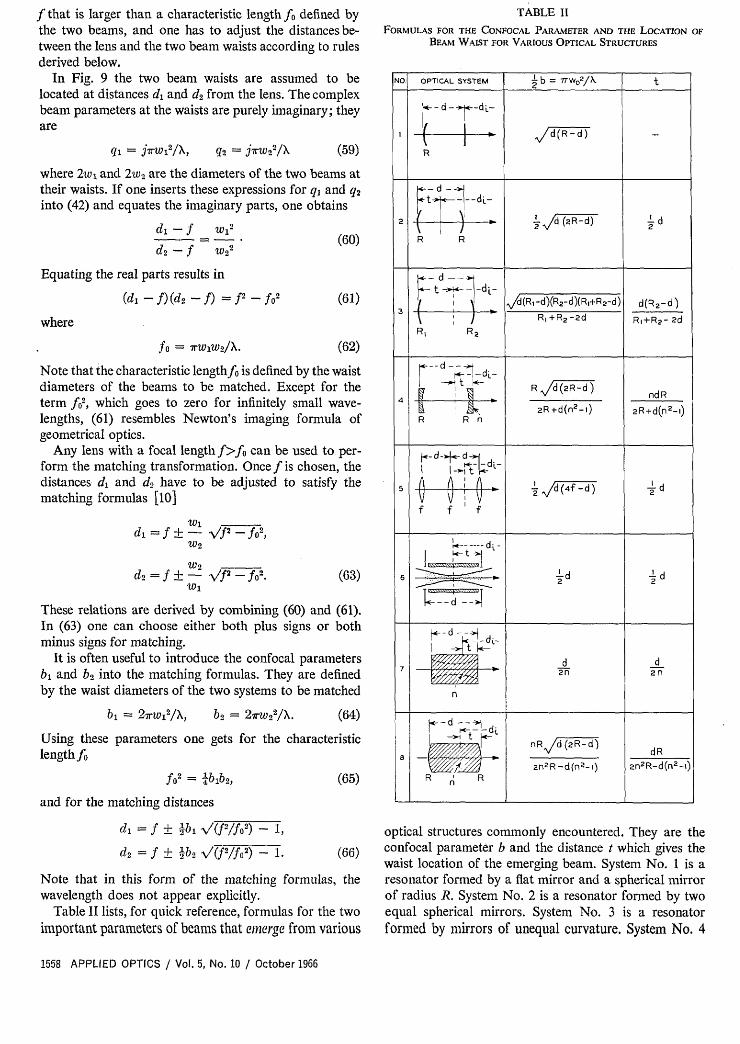
TABLE II

FORMULAS FOR THE CONFOCAL PARAMETER AND THE LOCATION OFBEAM WAIST FOR VARIOUS OPTICAL STRUCTURES

di = 1 f ± _2b1 (f 2/fo 2 )-1,

= f + 2b2 V(f2/fa2) - 1. (66)

Note that in this form of the matching formulas, thewavelength does not appear explicitly.

Table II lists, for quick reference, formulas for the twoimportant parameters of beams that emerge from various

optical structures commonly encountered. They are theconfocal parameter b and the distance t which gives thewaist location of the emerging beam. System No. 1 is aresonator formed by a flat mirror and a spherical mirrorof radius R. System No. 2 is a resonator formed by twoequal spherical mirrors. System No. 3 is a resonatorformed by mirrors of unequal curvature. System No. 4


bi °= 27rw,2/X,

I

0

-b f I

_

_ / \ N1

1.0

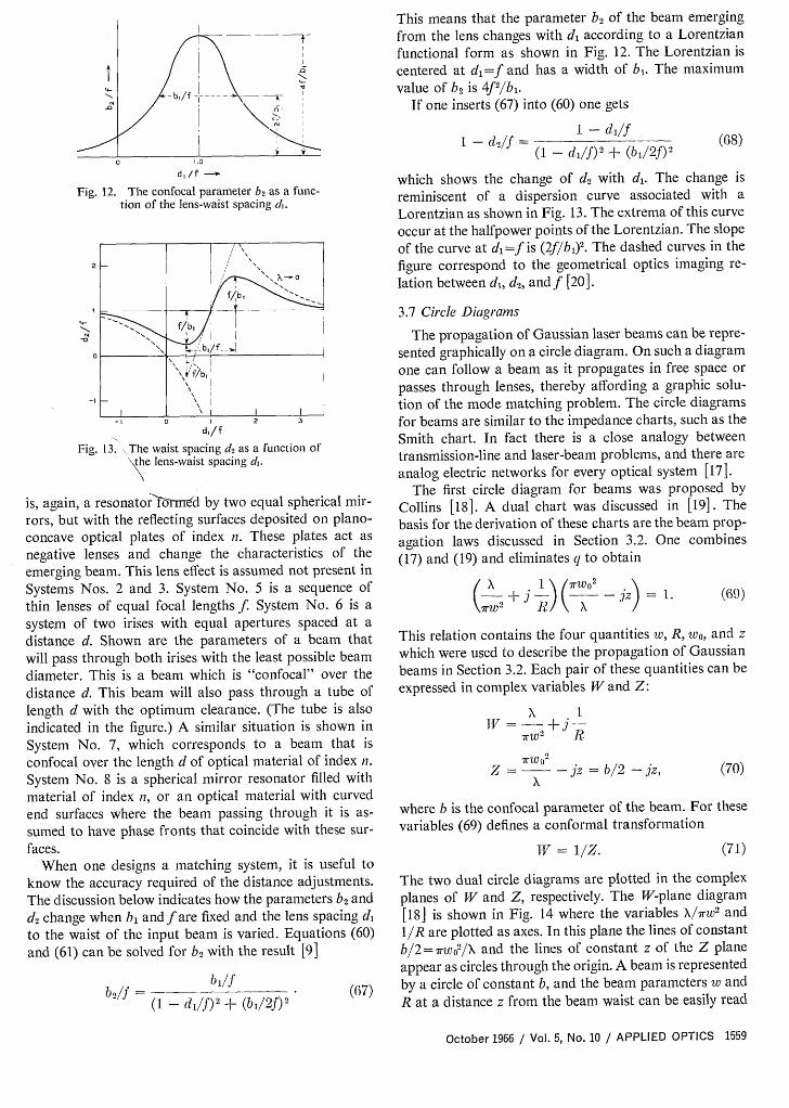
d,/fFig. 12. The confocal parameter b2 as a func-

tion of the lens-waist spacing di.

2 / ,I

- ____

s I 0 1 2 3

d,/fFig. 13. .The waist spacing d2 as a function of

the lens-waist spacing di,.

is, again, a resonator-ror-md by two equal spherical mir-rors, but with the reflecting surfaces deposited on plano-concave optical plates of index n. These plates act asnegative lenses and change the characteristics of theemerging beam. This lens effect is assumed not present inSystems Nos. 2 and 3. System No. 5 is a sequence ofthin lenses of equal focal lengths f. System No. 6 is asystem of two irises with equal apertures spaced at adistance d. Shown are the parameters of a beam thatwill pass through both irises with the least possible beamdiameter. This is a beam which is "confocal" over thedistance d. This beam will also pass through a tube oflength d with the optimum clearance. (The tube is alsoindicated in the figure.) A similar situation is shown in

System No. 7, which corresponds to a beam that isconfocal over the length d of optical material of index n.System No. 8 is a spherical mirror resonator filled withmaterial of index n, or an optical material with curvedend surfaces where the beam passing through it is as-sumed to have phase fronts that coincide with these sur-faces.

When one designs a matching system, it is useful toknow the accuracy required of the distance adjustments.The discussion below indicates how the parameters b2 andd2 change when bi andf are fixed and the lens spacing dito the waist of the input beam is varied. Equations (60)and (61) can be solved for b2 with the result [9]

bl/fb2/f - (1 - d/f) 2 + (bl/2f) 2 (67)

This means that the parameter b2 of the beam emergingfrom the lens changes with d according to a Lorentzianfunctional form as shown in Fig. 12. The Lorentzian iscentered at d1 =f and has a width of bl. The maximumvalue of b2 is 4f 2/b1 .

If one inserts (67) into (60) one gets

1 - d2/f =1 - d/f

(1 - df) 2 + (b1/2f)2 (68)

which shows the change of d2 with d. The change isreminiscent of a dispersion curve associated with aLorentzian as shown in Fig. 13. The extrema of this curveoccur at the halfpower points of the Lorentzian. The slopeof the curve at d 1 =f is (2f/b 1)2 . The dashed curves in thefigure correspond to the geometrical optics imaging re-lation between di, d2, and f [20].

3.7 Circle Diagrams

The propagation of Gaussian laser beams can be repre-sented graphically on a circle diagram. On such a diagramone can follow a beam as it propagates in free space orpasses through lenses, thereby affording a graphic solu-tion of the mode matching problem. The circle diagramsfor beams are similar to the impedance charts, such as theSmith chart. In fact there is a close analogy betweentransmission-line and laser-beam problems, and there areanalog electric networks for every optical system [17].

The first circle diagram for beams was proposed byCollins [18]. A dual chart was discussed in [19]. Thebasis for the derivation of these charts are the beam prop-agation laws discussed in Section 3.2. One combines(17) and (19) and eliminates q to obtain

X I /7rW02 \(w~fj X V-X--jz) = 1.Irw2R R"X-/

(69)

This relation contains the four quantities w, R, w0, and zwhich were used to describe the propagation of Gaussianbeams in Section 3.2. Each pair of these quantities can beexpressed in complex variables W and Z:

1IV =-- +j-

7rw2 R

7rWo2

Z = -jz = b/2-jz,X

(70)

where b is the confocal parameter of the beam. For thesevariables (69) defines a conformal transformation

IV = I/Z. (71)

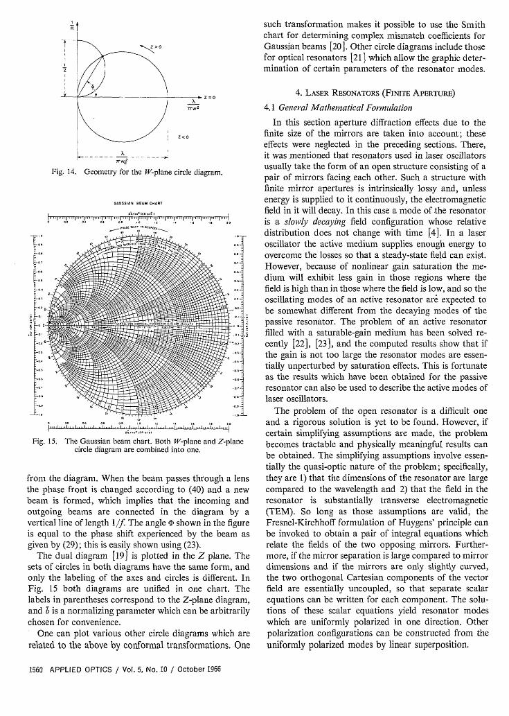
The two dual circle diagrams are plotted in the complexplanes of W and Z, respectively. The W-plane diagram[18] is shown in Fig. 14 where the variables X/7rw2 andI/R are plotted as axes. In this plane the lines of constantb/2=7rw 2/X and the lines of constant z of the Z planeappear as circles through the origin. A beam is representedby a circle of constant b, and the beam parameters w andR at a distance z from the beam waist can be easily read


R

Z

2>"~~,0

~~~~~~~~z~0x x I

77W2W

2<0

Fig. 14. Geometry for the W-plane circle diagram.

GAUSSIAN BEAM CHART

iO . 1 1 1 -b} , 11 ... p - . Cr I¢ ... I ,I ... I ... I20.

0 O.. ... . . I ~~~~~~~~~~ . . I ,, .1.,..-O, ,

Fig. 15, The Gaussian beam chart. Both W-plane and Z-planecircle diagram are combined into one.

from the diagram. When the beam passes through a lensthe phase front is changed according to (40) and a newbeam is formed, which implies that the incoming andoutgoing beams are connected in the diagram by avertical line of length I/f. The angle cP shown in the figureis equal to the phase shift experienced by the beam asgiven by (29); this is easily shown using (23).

The dual diagram [19] is plotted in the Z plane. Thesets of circles in both diagrams have the same form, andonly the labeling of the axes and circles is different. InFig. 15 both diagrams are unified in one chart. Thelabels in parentheses correspond to the Z-plane diagram,and is a normalizing parameter which can be arbitrarilychosen for convenience.

One can plot various other circle diagrams which arerelated to the above by conformal transformations. One

such transformation makes it possible to use the Smithchart for determining complex mismatch coefficients forGaussian beams [20 ]. Other circle diagrams include thosefor optical resonators [211 which allow the graphic deter-mination of certain parameters of the resonator modes.

4. LASER RESONATORS (FINITE APERTURE)

4.1 General Mathematical Formulation

In this section aperture diffraction effects due to thefinite size of the mirrors are taken into account; theseeffects were neglected in the preceding sections. There,it was mentioned that resonators used in laser oscillatorsusually take the form of an open structure consisting of apair of mirrors facing each other. Such a structure withfinite mirror apertures is intrinsically lossy and, unlessenergy is supplied to it continuously, the electromagneticfield in it will decay. In this case a mode of the resonatoris a slowly decaying field configuration whose relativedistribution does not change with time [4]. In a laseroscillator the active medium supplies enough energy toovercome the losses so that a steady-state field can exist.However, because of nonlinear gain saturation the me-dium will exhibit less gain in those regions where thefield is high than in those where the field is low, and so theoscillating modes of an active resonator are expected tobe somewhat different from the decaying modes of thepassive resonator. The problem of an active resonatorfilled with a saturable-gain medium has been solved re-cently [22], [23], and the computed results show that ifthe gain is not too large the resonator modes are essen-tially unperturbed by saturation effects. This is fortunateas the results which have been obtained for the passiveresonator can also be used to describe the active modes oflaser oscillators.

The problem of the open resonator is a difficult oneand a rigorous solution is yet to be found. However, ifcertain simplifying assumptions are made, the problembecomes tractable and physically meaningful results canbe obtained. The simplifying assumptions involve essen-tially the quasi-optic nature of the problem; specifically,they are 1) that the dimensions of the resonator are largecompared to the wavelength and 2) that the field in theresonator is substantially transverse electromagnetic(TEM). So long as those assumptions are valid, theFresnel-Kirchhoff formulation of Huygens' principle canbe invoked to obtain a pair of integral equations whichrelate the fields of the two opposing mirrors. Further-more, if the mirror separation is large compared to mirrordimensions and if the mirrors are only slightly curved,the two orthogonal Cartesian components of the vectorfield are essentially uncoupled, so that separate scalarequations can be written for each component. The solu-tions of these scalar equations yield resonator modeswhich are uniformly polarized in one direction. Otherpolarization configurations can be constructed from theuniformly polarized modes by linear superposition.


4-

MIRROR I

. s MIRROR 2

2a1 - _ - - 2a 2 -

.- d

OPAQUE ABSORBING SCREENS

4 d - d - A

LENS

-2a~ - 2 - -2a, --- 2a - __

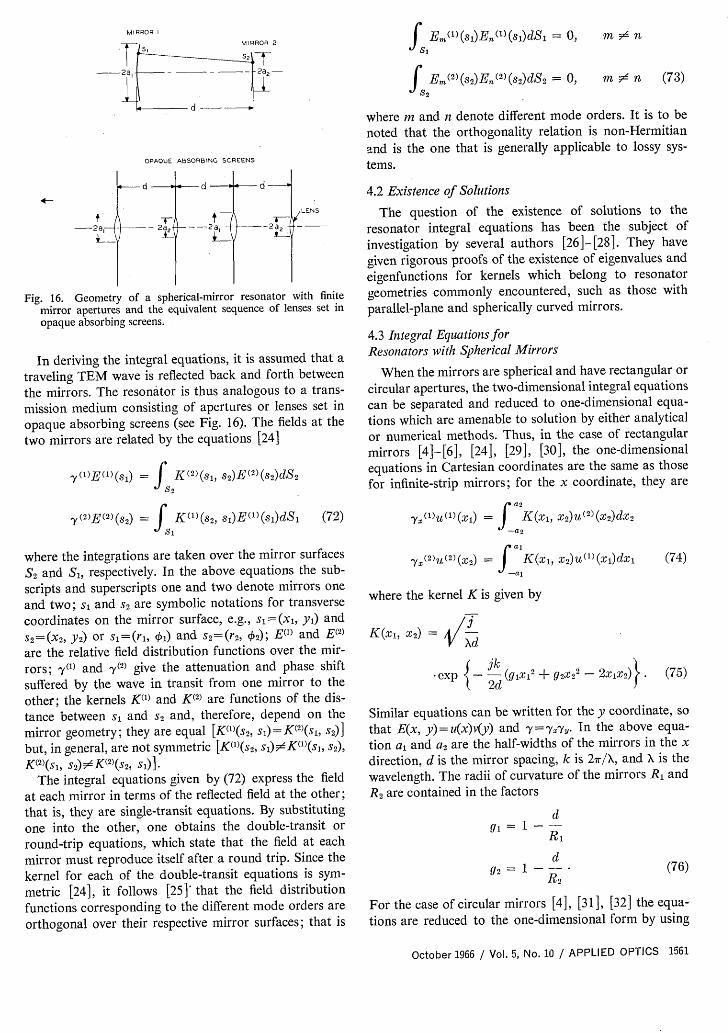
Fig. 16. Geometry of a spherical-mirror resonator with finite

mirror apertures and the equivalent sequence of lenses set inopaque absorbing screens.

In deriving the integral equations, it is assumed that a

traveling TEM wave is reflected back and forth between

the mirrors. The resonator is thus analogous to a trans-

mission medium consisting of apertures or lenses set in

opaque absorbing screens (see Fig. 16). The fields at the

two mirrors are related by the equations [24]

y(t)E(l)(si) = f Kl)(sl, s2)E(2)(s2)dS2S2

(2 )E (2)(S2)= K(')(s2 , sI)E(1)(si)dSi (72)Si

where the integrations are taken over the mirror surfaces

S2 and S1, respectively. In the above equations the sub-

scripts and superscripts one and two denote mirrors one

and two; si and s2 are symbolic notations for transverse

coordinates on the mirror surface, e.g., sl=(xi, yi) and

S2 =(X2 , y2) or si=(r,, 'k,) and s2=(r 2 , 42); E(') and E(2)

are the relative field distribution functions over the mir-

rors; 7ytl) and ya(2) give the attenuation and phase shift

suffered by the wave in transit from one mirror to the

other; the kernels K(1) and K(2) are functions of the dis-

tance between s1 and S2 and, therefore, depend on the

mirror geometry; they are equal [K(t)(s2, sl)=K(2)(sI, S2)]

but, in general, are not symmetric [K(l)(s2, si)KK(')(s1 , S2),

K(2)(Sl, s2) 5dK(2) (S2 S)]-

The integral equations given by (72) express the field

at each mirror in terms of the reflected field at the other;

that is, they are single-transit equations. By substitutingone into the other, one obtains the double-transit or

round-trip equations, which state that the field at each

mirror must reproduce itself after a round trip. Since the

kernel for each of the double-transit equations is sym-

metric [24], it follows [25]' that the field distribution

functions corresponding to the different mode orders are

orthogonal over their respective mirror surfaces; that is

f Em(l)(s)En.()(sI)dSi = 0,

j Em(2)(S2)E (2)(S2)dS2 = 0,s2

m F ( n

m 5 n (73)

where m and n denote different mode orders. It is to be

noted that the orthogonality relation is non-Hermitianand is the one that is generally applicable to lossy sys-

tems.

4.2 Existence of Solutions

The question of the existence of solutions to the

resonator integral equations has been the subject of

investigation by several authors [26]-[28]. They havegiven rigorous proofs of the existence of eigenvalues and

eigenfunctions for kernels which belong to resonatorgeometries commonly encountered, such as those withparallel-plane and spherically curved mirrors.

4.3 Integral EquationsforResonators with Spherical Mirrors

When the mirrors are spherical and have rectangular or

circular apertures, the two-dimensional integral equationscan be separated and reduced to one-dimensional equa-tions which are amenable to solution by either analyticalor numerical methods. Thus, in the case of rectangularmirrors [4]-[6], [24], [29], [30], the one-dimensionalequations in Cartesian coordinates are the same as thosefor infinite-strip mirrors; for the x coordinate, they are

,(l)U(l)(xI) = j K(x, x2)u(2)(x2)dx2- 2

(74)

where the kernel K is given by

K(x1, X2) = Vxd

*exp {- (gqX12 + 2X22 - 2xlX2 )}. (75)

Similar equations can be written for the y coordinate, so

that E(x, y)=u(x)v(y) and y-=Tyxy. In the above equa-

tion a, and a2 are the half-widths of the mirrors in the x

direction, d is the mirror spacing, k is 2 r/X, and X is thewavelength. The radii of curvature of the mirrors R1 and

R 2 are contained in the factors

d,9= 1 - -

d92 = 1 --

R2(76)

For the case of circular mirrors [4], [31], [32] the equa-

tions are reduced to the one-dimensional form by using


(2) U (2) (2) = K(x, X2 )u(')(xl)dxi

cylindrical coordinates and by assuming a sinusoidalazimuthal variation of the field; that is, E(r, 4) = R1(r)e-i0.The radial distribution functions R1 IM and R1(2) satisfy theone-dimensional integral equations:

Yz ()2Rz(1)(ri)-\'ri = a2 KI(ri, r 2 )Rz(2)(r 2 )-/r2 dr20

7i 2 )R t 2 (r2)v'r 2 = KI(r, r2)R(')(r) Vrdr (77)

where the kernel K, is given by

3 , rir2~K1(r1, r2) = ,k -) -\/lr

d( d

*exp *- - (glr12 + q2r22)I!- 2d +g2r-' (78)

same resonant frequency, and mode patterns that arescaled versions of each other. Thus, the equivalence rela-tions reduce greatly the number of calculations which arenecessary for obtaining the solutions for the variousresonator geometries.

4.5 Stability Condition and Diagram

Stability of optical resonators has been discussed inSection 2 in terms of geometrical optics. The stabilitycondition is given by (8). In terms of the stability factorsG1 and G2, it is

0 < G1 G2 < 1

or

0 < 9192 < 1. (80)

and Jz is a Bessel function of the first kind and th order.In (77), a, and a2 are the radii of the mirror apertures andd is the mirror spacing; the factors gi and g2 are given by(76).

Except for the special case of the confocal resonator[5] (gl=g2=0), no exact analytical solution has beenfound for either (74) or (77), but approximate methodsand numerical techniques have been employed with suc-cess for their solutions. Before presenting results, it isappropriate to discuss two important properties whichapply in general to resonators with spherical mirrors;these are the properties of "equivalence" and "stability."

4.4 Equivalent Resonator Systems,

The equivalence properties [24], [331 of spherical-mirror resonators are obtained by simple algebraic manip-ulations of the integral equations. First, it is obvious thatthe mirrors can be interchanged without affecting theresults; that is, the subscripts and superscripts one andtwo can be interchanged. Second, the diffraction loss andthe intensity pattern of the mode remain invariant if bothgi and g2 are reversed in sign; the eigenfunctions E andthe eigenvalues y merely take on complex conjugatevalues. An example of such equivalent systems is that ofparallel-plane (gl=g2=1) and concentric (gl=g2=-1)resonator systems.

The third equivalence property involves the Fresnelnumber N and the stability factors G1 and G2, where

a a2

xd

alG1= a'-

a2

G2 = 2-* (79)a,

If these three parameters are the same for any two resona-tors, then they would have the same diffraction loss, the

Resonators are stable if this condition is satisfied andunstable otherwise.

A stability diagram [6], [24] for the various resonatorgeometries is shown in Fig. 4 where gi and g2 are the co-ordinate axes and each point on the diagram represents aparticular resonator geometry. The boundaries betweenstable and unstable (shaded) regions are determined by(80), which is based on geometrical optics. The fields ofthe modes in stable resonators are more concentratednear the resonator axes than those in unstable resonatorsand, therefore, the diffraction losses of unstable resona-tors are much higher than those of stable resonators. Thetransition, which occurs near the boundaries, is gradualfor resonators with small Fresnel numbers and moreabrupt for those with large Fresnel numbers. The originof the diagram represents the confocal system with mirrorsof equal curvature (R 1=R 2=d) and is a point of lowestdiffraction loss for a given Fresnel number. The fact thata system with minor deviations from the ideal confocalsystem may become unstable should be borne in mindwhen designing laser resonators.

4.6 Modes of the Resonator

The transverse field distributions of the resonatormodes are given by the eigenfunctions of the integralequations. As yet, no exact analytical solution has beenfound for the general case of arbitrary G and G2, butapproximate analytical expressions have been obtained todescribe the fields in stable spherical-mirror resonators[51, [6]. These approximate eigenfunctions are the sameas those of the optical beam modes which are discussed inSection 2; that is, the field distributions are given approxi-mately by Hermite-Gaussian functions for rectangularmirrors [5], [6], [34], and by Laguerre-Gaussian func-tions for circular mirrors [6], [7]. The designation of theresonator modes is given in Section 3.5. (The modes aredesignated as TEMmnq for rectangular mirrors andTEMPI, for circular mirrors.) Figure 7 shows photo-graphs of some of the rectangular mode patterns of a


_ .,I 1l, I, l7 *1+ iAissi.,TEM,, TEM,, TEM20

f . I 1 I1

TEM,, TEM,, TEM,,

'4 t it t II

TEM,, TEM,2 TEM,,

SQUARE MIRRORS

TEM,,

( t 4;

TEMQ

TEM20

TEMo,

I i L I

TEM21

TEM0 2

ilTEM,,

TEM22

CIRCULAR MIRRORS

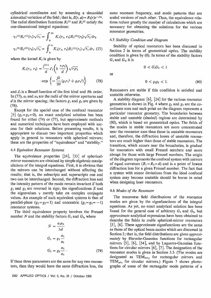
Fig. 17. Linearly polarized resonator mode configurationsfor square and circular mirrors.

I

I

+X

+m

=FR

Fig. 18. Synthesis of different polarization configurationsfrom the linearly polarized TEMO mode.

laser. Linearly polarized mode configurations for squaremirrors and for circular mirrors are shown in Fig. 17.By combining two orthogonally polarized modes of thesame order, it is possible to synthesize other polarizationconfigurations; this is shown in Fig. 18 for the TEMolmode.

Field distributions of the resonator modes for anyvalue of G could be obtained numerically by solving theintegral equations either by the method of successive ap-proximations [4], [24], [31] or by the method of kernelexpansion [30], [32]. The former method of solution isequivalent to calculating the transient behavior of theresonator when it is excited initially with a wave of arbi-trary distribution. This wave is assumed to travel backand forth between the mirrors of the resonator, under-going changes from transit to transit and losing energy bydiffraction. After many transits a quasi steady-state con-dition is attained where the fields for successive transits

differ only by a constant multiplicative factor. This steady-state relative field distribution is then an eigenfunction ofthe integral equations and is, in fact, the field distribu-tion of the mode that has the lowest diffraction loss forthe symmetry assumed (e.g., for even or odd symmetry inthe case of infinite-strip mirrors, or for a given azimuthalmode index number I in the case of circular mirrors); theconstant multiplicative factor is the eigenvalue associatedwith the eigenfunction and gives the diffraction loss andthe phase shift of the mode. Although this simple formof the iterative method gives only the lower order solu-tions, it can, nevertheless, be modified to yield higherorder ones [24], 135]. The method of kernel expansion,however, is capable of yielding both low-order and high-order solutions.

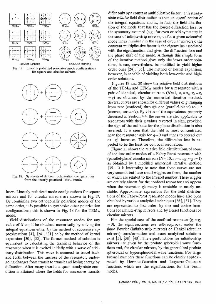
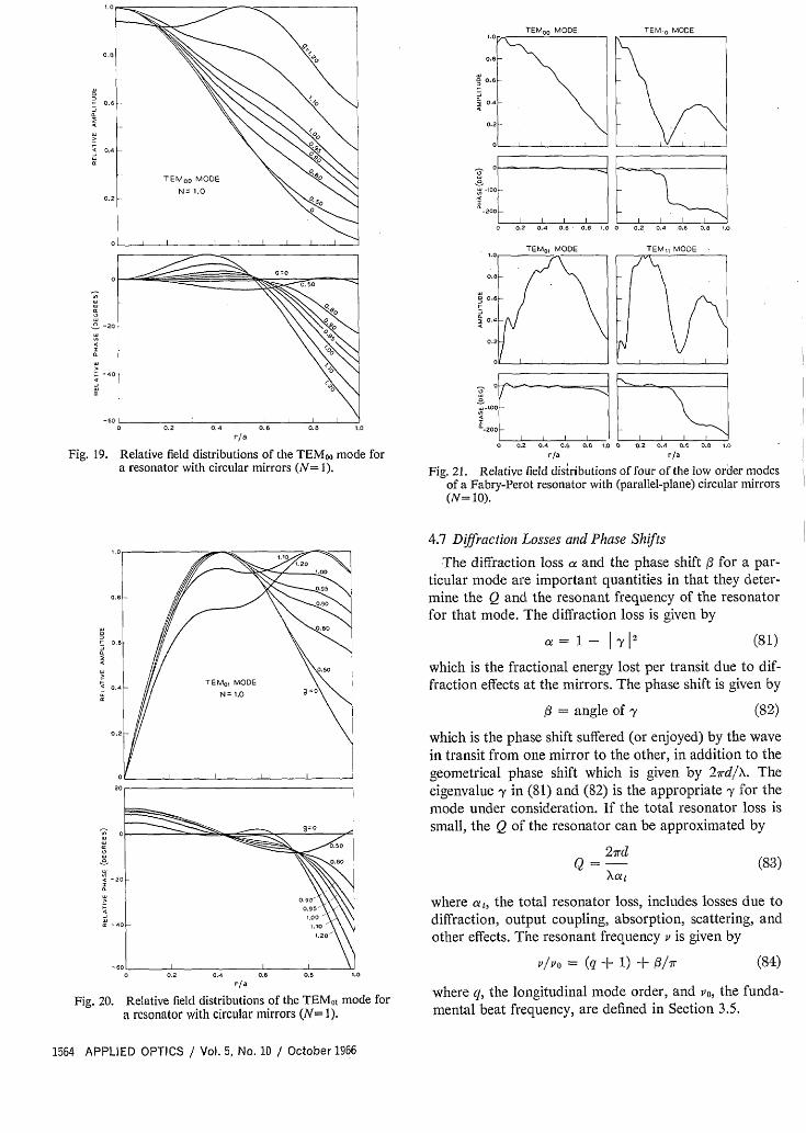
Figures 19 and 20 show the relative field distributionsof the TEM0 0 and TEMo modes for a resonator with apair of identical, circular mirrors (N=o1, al=a 2, gl=g2

= g) as obtained by the numerical iterative method.Several curves are shown for different values of g, rangingfrom zero (confocal) through one (parallel-plane) to 1.2(convex, unstable). By virtue of the equivalence propertydiscussed in Section 4.4, the curves are also applicable toresonators with their g values reversed in sign, providedthe sign of the ordinate for the phase distribution is alsoreversed. It is seen that the field is most concentratednear the resonator axis for g=0 and tends to spread outas Ig increases. Therefore, the diffraction loss is ex-pected to be the least for confocal resonators.

Figure 21 shows the relative field distributions of someof the low order modes of a Fabry-Perot resonator with(parallel-plane) circular mirrors (N= 10, a1 = a2, gl =g2 = 1)as obtained by a modified numerical iterative method[35]. It is interesting to note that these curves are notvery smooth but have small wiggles on them, the numberof which are related to the Fresnel number. These wigglesare entirely absent for the confocal resonator and appearwhen the resonator geometry is unstable or nearly un-stable. Approximate expressions for the field distribu-tions of the Fabry-Perot resonator modes have also beenobtained by various analytical techniques [36], [37]. Theyare represented to first order, by sine and cosine func-tions for infinite-strip mirrors and by Bessel functions forcircular mirrors.

For the special case of the confocal resonator (gl-=g2= 0), the eigenfunctions are self-reciprocal under the

finite Fourier (infinite-strip mirrors) or Hankel (circularmirrors) transformation and exact analytical solutionsexist [5], [38]-[40]. The eigenfunctions for infinite-stripmirrors are given by the prolate spheroidal wave func-tions and, for circular mirrors, by the generalized prolatespheroidal or hyperspheroidal wave functions. For largeFresnel numbers these functions can be closely approxi-mated by Hermite-Gaussian and Laguerre-Gaussianfunctions which are the eigenfunctions for the beammodes.


TEM0 0 MODE TEM 1 MODE

.6

.2 L

0'L~~~~~~~~~~~~~~~~~~~~~~~~~~~~~~~~~~~~~

00 VL I I I~~~~~~J 0 0.2 0.4 .6 0.6 .00 0.2 0.4 0.0 0.0 1.0

TEMQ, MODE TEM,, MODE

.0

0.2 NO 1.0

-600 0.2 0.4 0.6 0.8 1.0

r/a

Fig. 19. Relative field distributions of the TEMoo mode fora resonator with circular mirrors (N= 1).

-2

o

ZI'C-zo0

0 0.2 0.4 0.6 O.6 1.0 0 0.2 0.4 0.6 O.8 1.0

r/a r/a

Fig. 21. Relative field distributions of four of the low order modesof a Fabry-Perot resonator with (parallel-plane) circular mirrors(N = 10).

4.7 Diffraction Losses and Phase Shifts

The diffraction loss a and the phase shift for a par-ticular mode are important quantities in that they deter-mine the Q and the resonant frequency of the resonatorfor that mode. The diffraction loss is given by

ao= l- Y12 (81)

which is the fractional energy lost per transit due to dif-fraction effects at the mirrors. The phase shift is given by

/3 = angle of y

0 0.2 0.4 0.6 0.5 1.0

r/a

Fig. 20. Relative field distributions of the TEMot mode fora resonator with circular mirrors (N= 1).

(82)

which is the phase shift suffered (or enjoyed) by the wavein transit from one mirror to the other, in addition to thegeometrical phase shift which is given by 2rd/X. Theeigenvalue -y in (81) and (82) is the appropriate -y for themode under consideration. If the total resonator loss issmall, the Q of the resonator can be approximated by

27rdQ = -- (83)

where ca,, the total resonator loss, includes losses due todiffraction, output coupling, absorption, scattering, andother effects. The resonant frequency v is given by

v/v = (q + 1) + o/h (84)

where q, the longitudinal mode order, and Po, the funda-mental beat frequency, are defined in Section 3.5.


' .0

-... I 2==._ - _

TEMo, MODE TEM lo MODE

I

AI

CiI

I

I I , ,

0

6

0

(L

0.6

0.4

0.21

0.10

0.06

0.04

0.02

0.01 I I I 1 I 1 L 1 1 1 1 \ i . '

0.1 0.2 0.4 0.6 1.0 2 4 6 10 20 40 60 100

N= a2/Xd

Fig. 22. Diffraction loss per transit (in decibels) for the TEMoomode of a stable resonator with circular mirrors.

0

0

0.1 0.2 0.4 0.6 1.0 2 4 6 10 20 40 60 100

N= a2/Xd

Fig. 23. Diffraction loss per transit (in decibels) for the TEMoimode of a stable resonator with circular mirrors.

The diffraction losses for the two lowest order (TEMooand TEMoi) modes of a stable resonator with a pair ofidentical, circular mirrors (ai=a2 , gl=g2=g) are givenin Figs. 22 and 23 as functions of the Fresnel number Nand for various values of g. The curves are obtained bysolving (77) numerically using the method of successiveapproximations [31 ]. Corresponding curves for the phaseshifts are shown in Figs. 24 and 25. The horizontal por-tions of the phase shift curves can be calculated from theformula

d = (2p + I + 1) arc cos -go12

0.11 1 ! I I I, 1 1 1 1 1 1 I I I

0.1 0.2 0.4 0.6 1.0 2 4 6 10 20 40 60

N= a2/Xd

Fig. 24. Phase shift per transit for the TEMoi mode of astable resonator with circular mirrors.

400

200 9 -

100 D

620 - 0a 9

0.1 0.2 0.4 0.6 1.0 2 4 6 10 20 40 60 100

Fig. 25. Phase shift per transit for the TEM00 mode of astable resonator with circullar mirrors.

while the phase-shift curves are for positive g only; thephase shift for negative g is equal to 180 degrees minusthat for positive g.

Analytical expressions for the diffraction loss and thephase shift have been obtained for the special cases ofparallel-plane (g =1.0) and confocal (g= 0) geometries

when the Fresnel number is either very large (small dif-fraction loss) or very small (large diffraction loss) [36],[38], [39], [41], [42]. In the case of the parallel-planeresonator with circular mirrors, the approximate expres-sions valid for large N, as derived by Vainshtein [36], are

for 91 = 2 (85)

which is equal to the phase shift for the beam modesderived in Section 3.5. It is to be noted that the loss curvesare applicable to both positive and negative values of g

a = 8'1 - (A + a) [(Sit + a)2 + 2] 2

/1fA = a-I a


= (2p + + 1) arc cos g, (86)

(87)

where 3=0.824, M= /8lrN, and Kp is the (p+)th zeroof the Bessel function of order . For the confocal resona-tor with circular mirrors, the corresponding expressionsare [39]

27r(8wN) 2p+1+le-4,IN

p!(p + + 1)!

/ = (2p + + 1)

+ (2r)] (88)

(89)

Similar expressions exist for resonators with infinite-stripor rectangular mirrors [36], [39]. The agreement be-tween the values obtained from the above formulas andthose from numerical methods is excellent.

The loss of the lowest order (TEMoo) mode of anunstable resonator is, to first order, independent of themirror size or shape. The formula for the loss, which isbased on geometrical optics, is [12]

1 - N1 - (9192)'a= 1 ±1 + \-(99)

(90)

where the plus sign in front of the fraction applies for gvalues lying in the first and third quadrants of the stabilitydiagram, and the minus sign applies in the other two quad-rants. Loss curves (plotted vs. N) obtained by solving theintegral equations numerically have a ripply behaviorwhich is attributable to diffraction effects [24], [43]. I-low-ever, the average values agree well with those obtainedfrom (90).

5. CONCLUDING REMARKS

Space limitations made it necessary to concentrate thediscussion of this article on the basic aspects of laserbeams and resonators. It was not possible to include suchinteresting topics as perturbations of resonators, resona-tors with tilted mirrors, or to consider in detail the effectof nonlinear, saturating host media. Also omitted was adiscussion of various resonator structures other thanthose formed of spherical mirrors, e.g., resonators withcorner cube reflectors, resonators with output holes, orfiber resonators. Another important, but omitted, field isthat of mode selection where much research work is cur-rently in progress. A brief survey of some of these topicsis given in [44].

REFERENCES

[1] R. H. Dicke, "Molecular amplification and generation systemsand methods," U. S. Patent 2 851 652, September 9, 1958.

[2] A. M. Prokhorov, "Molecular amplifier and generator for sub-millimeter waves," JETP (USSR), vol. 34, pp. 1658-1659, June1958; Sov. Phys. JETP, vol. 7, pp. 1140-1141, December 1958.

[3] A. L. Schawlow and C. H. Townes, "Infrared and opticalmasers," Phys. Rev., vol. 29, pp. 1940-1949, December 1958.

[4] A. G. Fox and T. Li, "Resonant modes in an optical maser,"Proc. IRE(Correspondence), vol. 48, pp. 1904-1905, November1960; "Resonant modes in a maser interferometer," Bell .Sys.Tech. J., vol. 40, pp. 453-488, March 1961.

[5] G. D. Boyd and J. P. Gordon, "Confocal multimode resonatorfor millimeter through optical wavelength masers," Bell Sys.Tech. J., vol. 40, pp. 489-508, March 1961.

[6] G. D. Boyd and H. Kogelnik, "Generalized confocal resonatortheory," Bell Sys. Tech. J., vol. 41, pp. 1347-1369, July 1962.

[7] G. Goubau and F. Schwering, "On the guided propagation ofelectromagnetic wave beams," IRE Trans. o Antennas andPropagation, vol. AP-9, pp. 248-256, May 1961.

[8] J. R. Pierce, "Modes in sequences of lenses," Proc. Nat'l Acad.

Sci., vol. 47, pp. 1808-1813, November 1961.[9] G. Goubau, "Optical relations for coherent wave beams," in

Electromagnetic Theory and Antennas. New York: Macmillan,1963, pp. 907-918.

[10] H. Kogelnik, "Imaging of optical mode-Resonators withinternal lenses," Bell Sys. Tech. J., vol. 44, pp. 455-494, March1965.

[11] -, "On the propagation of Gaussian beams of light throughlenslike media including those with a loss or gain variation,"Appl. Opt., vol. 4, pp. 1562-1569, December 1965.

[12] A. E. Siegman, "Unstable optical resonators for laser applica-tions," Proc. IEEE, vol. 53, pp. 277-287, March 1965.

[13] W. Brower, Matrix Methods in Optical Istrument Design.New York: Benjamin, 1964. E. L. O'Neill, Itroduction to Sta-tistical Optics. Reading, Mass.: Addison-Wesley, 1963.

[14] M. Bertolotti, "Matrix representation of geometrical proper-ties of laser cavities," Nuovo Cimento, vol. 32, pp. 1242-1257,June 1964. V. P. Bykov and L. A. Vainshtein, "Geometricaloptics of open resonators," JETP (USSR), vol. 47, pp. 508-517, August 1964. B. Macke, "Laser cavities in geometricaloptics approximation," J. Pys. (Paris), vol. 26, pp. 104A-112A, March 1965. W. K. Kahn, "Geometric optical deriva-tion of formula for the variation of the spot size in a sphericalmirror resonator," Appl. Opt., vol. 4, pp. 758-759, June 1965.

[15] J. R. Pierce, Theory and Design of Electron Beams. New York:Van Nostrand, 1954, p. 194.

[16] H. Kogelnik and W. W. Rigrod, "Visual display of isolatedoptical-resonator modes," Proc. IRE (Correspondence), vol.50, p. 220, February 1962.

[17] G. A. Deschamps and P. E. Mast, "Beam tracing and applica-tions," in Proc. Symposium on Quasi-Optics. New York: Poly-technic Press, 1964, pp. 379-395.

[18] S. A. Collins, "Analysis of optical resonators involving focus-ing elements," Appl. Opt., vol. 3, pp. 1263-1275, November1964.

[19] T. Li, "Dual forms of the Gaussian beam chart," Appl. Opt.,vol. 3, pp. 1315-1317, November 1964.

[20] T. S. Chu, "Geometrical representation of Gaussian beampropagation," Bell Sys. Tech. J., vol. 45, pp. 287-299, Febru-ary 1966.

[21] J. P. Gordon, "A circle diagram for optical resonators," Bell

Sys. Tech. J., vol. 43, pp. 1826-1827, July 1964. M. J. Offer-haus, "Geometry of the radiation field for a laser interferom-eter," Philips Res. Rept., vol. 19, pp. 520-523, December 1964.

[22] H. Statz and C. L. Tang, "Problem of mode deformation inoptical masers," J. Appl. Phys., vol. 36, pp. 1816-1819, June1965.

[23] A. G. Fox and T. Li, "Effect of gain saturation on the oscillat-ing modes of optical masers," IEEE J. of Quantum Electronics,vol. QE-2, p. xii, April 1966.

[24] -- , "Modes in a maser interferometer with curved and tiltedmirrors," Proc. IEEE, vol. 51, pp. 80-89, January 1963.

[25] F. B. Hildebrand, Methods of Applied Mathematics. EnglewoodCliffs, N. J.: Prentice Hall, 1952, pp. 412-413.

[26] D. J. Newman and S. P. Morgan, "Existence of eigenvalues ofa class of integral equations arising in laser theory," Bell Sys.

Tech. J., vol. 43, pp. 113-126, January 1964.[27] J. A. Cochran, "The existence of eigenvalues for the integral

equations of laser theory," Bell Sys. Tech. J., vol. 44, pp. 77-88,January 1965.

[28] H. Hochstadt, "On the eigenvalue of a class of integral equa-tions arising in laser theory," SIAM Rev., vol. 8, pp. 62-65,January 1966.

[29] D. Gloge, "Calculations of Fabry-Perot laser resonators byscattering matrices," Arch. Elect. Ubertrag., vol. 18, pp. 197-203, March 1964.

[30] W. Streifer, "Optical resonator modes-rectangular reflectorsof spherical curvature," J. Opt. Soc. Ain., vol. 55, pp. 868-877,July 1965

[31] T. Li, "Diffraction loss and selection of modes in maser reso-nators with circular mirrors," Bell Sys. Tech. J., vol. 44, pp.917-932, May-June, 1965.

[32] J. C. Heurtley and W. Streifer, "Optical resonator modes-


circular reflectors of spherical curvature," J. Opt. Soc. Am.,vol. 55, pp. 1472-1479, November 1965.

[33] J. P. Gordon and H. Kogelnik, "Equivalence relations amongspherical mirror optical resonators," Bell Sys. Tech. J., vol.43, pp. 2873-2886, November 1964.

[34] F. Schwering, "Reiterative wave beams of rectangular sym-metry," Arch. Elect. bertrag., vol. 15, pp. 555-564, Decem-ber 1961

[35] A. G. Fox and T. Li, to be published.[36] L. A. Vainshtein, "Open resonators for lasers," JETP (USSR),

vol. 44, pp. 1050-1067, March 1963; Sov. Phys. JETP, vol. 17,pp. 709-719, September 1963.

[37] S. R. Barone, "Resonances of the Fabry-Perot laser," J. Appl.Phys., vol. 34, pp. 831-843, April 1963.

[38] D. Slepian and H. 0. Pollak, "Prolate spheroidal wave func-tions, Fourier analysis and uncertainty-I," Bell Sys. Tech. J.,vol. 40, pp. 43-64, January 1961.

[39] D. Slepian, "Prolate spheroidal wave functions, Fourier anal-

ysis and uncertainty-IV: Extensions to many dimensions;generalized prolate spheroidal functions," Bell Svs. Tech. J.,vol. 43, pp. 3009-3057, November 1964.

[40] J. C. Heurtley, "Hyperspheroidal functions-optical resonatorswith circular mirrors," in Proc. Symposium on Quasi-Optics.New York: Polytechnic Press, 1964, pp. 367-375.

[41] S. R. Barone and M. C. Newstein, "Fabry-Perot resonances atsmall Fresnel numbers," Appl. Opt., vol. 3, p. 1194, October1964.

[42] L. Bergstein and H. Schachter, "Resonant modes of optic cavi-ties of small Fresnel numbers," J. Opt. Soc. Am., vol. 55, pp.1226-1233, October 1965.

[431 A. G. Fox and T. Li, "Modes in a maser interferometer withcurved mirrors," in Proc. Third International Congress olQuantum Electronics. New York: Columbia University Press,1964, pp. 1263-1270.

[44] H. Kogelnik, "Modes in optical resonators," in Lasers,A. K. Levine, Ed. New York: Dekker, 1966.

Modes, Phase Shifts, and Losses of Flat-RoofOpen Resonators

P. F. CHECCACCI, ANNA CONSORTINI, AND ANNAMARIA SCHEGGI

Abstract-The integral Squation of a "flat-roof resonator" issolved by the Fox and Li method of iteration in a number of particularcases.

Mode patterns, phase shifts, and power losses are derived. A goodoverall agreement is found with the approximate theory previouslydeveloped by Toraldo di Francia.

Some experimental tests carried out on a microwave model give afurther confirmation of the theoretical predictions.

I. INTRODUCTION

A PARTICULAR type of open resonator terminatedby roof reflectors with very small angles, the so-called "flat-roof resonator" (Fig. 1) was recently

described by Toraldo di Francia [1].The mathematical approach consisted in considering

the solutions of the wave equation (for the electric ormagnetic field) in the two halves of a complete "diamondcavity" whose normal cross section is shown in Fig. 2,ignoring the fact that the reflectors are finite.

The two half-cavities were referred to cylindrical co-ordinates centered at G and H, respectively, and solutionswere given in terms of high-order cylindrical waves. Thefield in the two half-cavities was matched over the median

Manuscript received May 4, 1966. The research reported herewas supported in part by the Air Force Cambridge Research Labo-ratories through the European Office of Aerospace Research (OAR),U. S. Air Force, under Contract AF 61(052)-871.

The authors are with the Centro Microonde, Consiglio Na-zionale delle Ricerche, Florence, Italy.

Fig. 1. The flat-roof resonator.

B

4:H-- __ | ___- H -

E

Fig. 2. The diamond cavity.

plane BE by simply requiring that this plane coincidewith a node or an antinode. Obviously the a angle of theroof must be so small that the curvature of the nodal orantinodal surfaces can be neglected. Due to the high orderof the cylindrical waves, the field in the central region ofthe cavity approaches the form of a standing wave be-tween the two roof reflectors, while it decays so rapidlyfrom the central region toward the vertices G and H,that the absence of the complete metal walls of the dia-mond outside the resonator will have very little impor-tance. This treatment, although approximate, allowed theauthor to understand how the resonator actually worked


Laser Beams and Resonators - physics.byu.edu beams and resonators, ... this will be discussed in...

Documents

Transcript of Laser Beams and Resonators - physics.byu.edu beams and resonators, ... this will be discussed in...