To appear in: The International Journal of Computer Vision

Large Occlusion Stereo

Aaron F. Bobick and Stephen S. Intille

bobick@media.mit.edu and intille@media.mit.edu

The Media Laboratory

Massachusetts Institute of Technology

20 Ames St., Cambridge MA 02139

Abstract: A method for solving the stereo matching problem in the presence of large occlusion is

presented. A data structure | the disparity space image | is de�ned to facilitate the description of

the e�ects of occlusion on the stereo matching process and in particular on dynammic programming

(DP) solutions that �nd matches and occlusions simultaneously. We signi�cantly improve upon existing

DP stereo matching methods by showing that while some cost must be assigned to unmatched pixels,

sensitivity to occlusion-cost and algorithmic complexity can be signi�cantly reduced when highly-

reliable matches, or ground control points, are incorporated into the matching process. The use of

ground control points eliminates both the need for biasing the process towards a smooth solution and

the task of selecting critical prior probabilities describing image formation. Finally, we describe how the

detection of intensity edges can be used to bias the recovered solution such that occlusion boundaries

will tend to be proposed along such edges, re ecting the observation that occlusion boundaries usually

cause intensity discontinuities.

Key words: stereo; occlusion; dynamic-programming stereo; disparity-space, ground-control points.

1 Introduction

Our world is full of occlusion. In any scene, we are likely to �nd several, if not several hundred, occlusion

edges. In binocular imagery, we encounter occlusion times two. Stereo images contain occlusion edges

that are found in monocular views and occluded regions that are unique to a stereo pair[7]. Occluded

regions are spatially coherent groups of pixels that can be seen in one image of a stereo pair but not in

the other. These regions mark discontinuities in depth and are important for any process which must

preserve object boundaries, such as segmentation, motion analysis, and object identi�cation. There is

psychophysical evidence that the human visual system uses geometrical occlusion relationships during

binocular stereopsis[28, 25, 1] to reason about the spatial relationships between objects in the world.

In this paper we present a stereo algorithm that does so as well.

Although absolute occlusion sizes in pixels depend upon the con�guration of the imaging system,

images of everyday scenes often contain occlusion regions much larger than those found in popular stereo

Figure 1: Noisy stereo pair of a man and kids. The largest occlusion region in this image is 93 pixels wide, or

13 percent of the image.

test imagery. In our lab, common images like Figure 1 contain disparity shifts and occlusion regions over

eighty pixels wide.1 Popular stereo test images, however, like the JISCT test set[9], the \pentagon"

image, the \white house" image, and the \Renault part" image have maximum occlusion disparity

shifts on the order of 20 pixels wide. Regardless of camera con�guration, images of the everyday world

will have substantially larger occlusion regions than aerial or terrain data. Even processing images with

small disparity jumps, researchers have found that occlusion regions are a major source of error[3].

Recent work on stereo occlusion, however, has shown that occlusion processing can be incorporated

directly into stereo matching[7, 18, 14, 21]. Stereo imagery contains both occlusion edges and occlusion

regions[18]. Occlusion regions are spatially coherent groups of pixels that appear in one image and

not in the other. These occlusion regions are caused by occluding surfaces and can be used directly in

stereo and occlusion reasoning.2

This paper divides into two parts. The �rst several sections concentrate on the recovery of stereo

matches in the presence of signi�cant occlusion. We begin by describing previous research in stereo

processing in which the possibility of unmatched pixels is included in the matching paradigm. Our

approach is to explicitly model occlusion edges and occlusion regions and to use them to drive the

matching process. We develop a data structure which we will call the disparity-space image (DSI),

and we use this data structure to describe the the dynamic-programming approach to stereo (as in

[18, 14, 19]) that �nds matches and occlusions simultaneously. We show that while some cost must be

incurred by a solution that proposes unmatched pixels, an algorithm's occlusion-cost sensitivity and

algorithmic complexity can be signi�cantly reduced when highly-reliable matches, or ground control

points (GCPs), are incorporated into the matching process. Experimental results demonstrate robust

behavior with respect to occlusion pixel cost if the GCP technique us employed.

The second logical part of the paper is motivated by the observation that monocular images also

contain information about occlusion. Di�erent objects in the world have varying texture, color, and

illumination. Therefore occlusion edges | jump edges between these objects or between signi�cantly

disparate parts of the same object | nearly always generate intensity edges in a monocular image. The

�nal sections of this paper consider the impact of intensity edges on the disparity space images and

extends our stereo technique to exploit information about intensity discontinuities. We note that recent

1Typical set up is two CCD cameras, with 12mm focal length lenses, separated by a baseline of about 30cm.2Belhumeur and Mumford [7] refer to these regions as \half-occlusion" areas as they are occluded from only one eye.However, since regions occluded from both eyes don't appear in any image, we �nd the distinction unneccesary hereand use \occluded region" to refer to pixels visible in only one eye.

2

psychophysical evidence strongly supports the importance of edges in the perception of occlusion.

2 Previous Occlusion and Stereo Work

Most stereo researchers have generally either ignored occlusion analysis entirely or treated it as a

secondary process that is postponed until matching is completed and smoothing is underway[4, 15].

A few authors have proposed techniques that indirectly address the occlusion problem by minimizing

spurious mismatches resulting from occluded regions and discontinuities[20, 11, 2, 26, 2, 24, 12].

Belhumeur has considered occlusion in several papers. In [7], Belhumeur and Mumford point out

that occluded regions, not just occlusion boundaries, must be identi�ed and incorporated into matching.

Using this observation and Bayefsian reasoning, an energy functional is derived using pixel intensity as

the matching feature, and dynamic programming is employed to �nd the minimal-energy solution. In

[5] and [6] the Bayesian estimator is re�ned to deal with sloping and creased surfaces. Penalty terms

are imposed for proposing a break in vertical and horizontal smoothness or a crease in surface slope.

Belhumeur's method requires the estimation of several critical prior terms which are used to suspend

smoothing operations.

Geiger, Ladendorf, and Yuille[18, 19] also directly address occlusion and occlusion regions by de�n-

ing an a priori probability for the disparity �eld based upon a smoothness function and an occlusion

constraint. For matching, two shifted windows are used in the spirit of [26] to avoid errors over discon-

tinuity jumps. Assuming the monotonicity constraint, the matching problem is solved using dynamic

programming. Unlike in Belhumeur's work, the stereo occlusion problem is formulated as a path-�nding

problem in a left-scanline to right-scanline matching space. Geiger et al. make explicit the observation

that \a vertical break (jump) in one eye corresponds to a horizontal break (jump) in the other eye."

Finally, Cox et al.[14] have proposed a dynamic programming solution to stereo matching that

does not require the smoothing term incorporated into Geiger and Belhumeur's work. They point out

that several equally good paths can be found through matching space using only the occlusion and

ordering constraints. To provide enough constraint for their system to select a single solution, they

optimize a Bayesian maximum-likelihood cost function minimizing inter- and intra-scanline disparity

discontinuities. The work of Cox et al. is the closest to the work we present here in that we also do

not exploit any explicit smoothness assumptions in our DP solution.

3 The DSI Representation

In this section we describe a data structure we call the disparity-space image, or DSI. We have used

the data structure to explore the occlusion and stereo problem and it facilitated our development of a

dynamic programming algorithm that uses occlusion constraints. The DSI is an explicit representation

of matching space; it is related to �gures that have appeared in previous work [26, 31, 13, 18, 19].

3.1 DSI Creation for Ideal Imagery

We generate the DSI representation for ith scanline in the following way: Select the ith scanline of the

left and right images, sLiand sR

irespectively, and slide them across one another one pixel at a time.

At each step, the scanlines are subtracted and the result is entered as the next line in the DSI. The

DSI representation stores the result of subtracting every pixel in sLiwith every pixel sR

iand maintains

the spatial relationship between the matched points. As such, it may be considered an (x, disparity)

matching space, with x along the horizontal, and disparity d along the vertical. Given two images IL

3

Right ImageLeft Image

Result: DSI iL

Crop

One pixel overlap (negative disparity)

Two pixel overlap (negative disparity)

N pixel overlap (zero disparity)

One pixel overlap (positive disparity)

.

.

.

.

.

.

.

.

.

.

.

.

Slide Right over Leftand subtract

scanline i

N N

scanline i

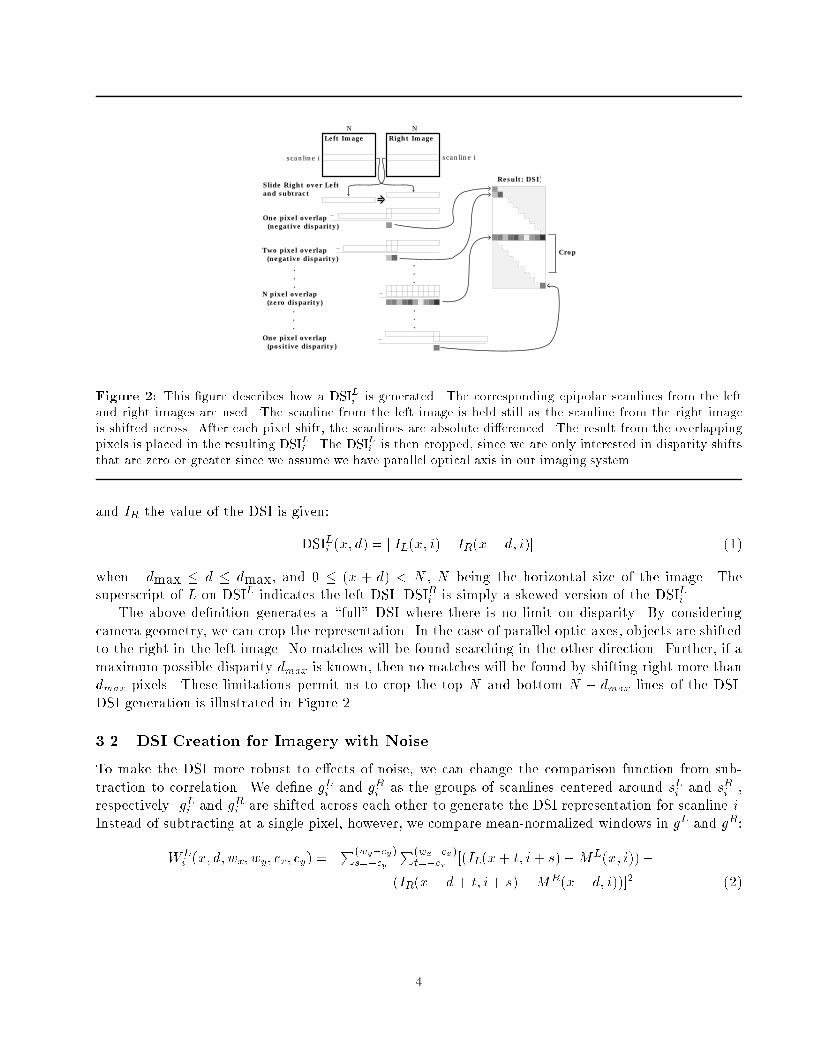
Figure 2: This �gure describes how a DSILiis generated. The corresponding epipolar scanlines from the left

and right images are used. The scanline from the left image is held still as the scanline from the right image

is shifted across. After each pixel shift, the scanlines are absolute di�erenced. The result from the overlapping

pixels is placed in the resulting DSILi . The DSIL

i is then cropped, since we are only interested in disparity shifts

that are zero or greater since we assume we have parallel optical axis in our imaging system.

and IR the value of the DSI is given:

DSILi(x; d) = kIL(x; i)� IR(x� d; i)k (1)

when �dmax � d � dmax, and 0 � (x + d) < N , N being the horizontal size of the image. The

superscript of L on DSIL indicates the left DSI. DSIRiis simply a skewed version of the DSIL

i.

The above de�nition generates a \full" DSI where there is no limit on disparity. By considering

camera geometry, we can crop the representation. In the case of parallel optic axes, objects are shifted

to the right in the left image. No matches will be found searching in the other direction. Further, if a

maximum possible disparity dmax is known, then no matches will be found by shifting right more than

dmax pixels. These limitations permit us to crop the top N and bottom N � dmax lines of the DSI.

DSI generation is illustrated in Figure 2.

3.2 DSI Creation for Imagery with Noise

To make the DSI more robust to e�ects of noise, we can change the comparison function from sub-

traction to correlation. We de�ne gLiand gR

ias the groups of scanlines centered around sL

iand sR

i,

respectively. gLiand gR

iare shifted across each other to generate the DSI representation for scanline i.

Instead of subtracting at a single pixel, however, we compare mean-normalized windows in gL and gR:

WL

i(x; d; wx; wy; cx; cy) =

P(wy�cy)s=�cy

P(wx�cx)t=�cx

[(IL(x+ t; i+ s)�ML(x; i))�

(IR(x� d+ t; i+ s)�MR(x� d; i))]2 (2)

4

Figure 3: To reduce the e�ects of noise in DSI generation, we have used 9 window matching, where window

centers (marked in black) are shifted to avoid spurious matches at occlusion regions and discontinuity jumps.

where wx�wy is the size of the window, (cx; cy) is the location of the reference point (typically the

center) of the window, and ML (MR) is the mean of the window in the left (right) image:

ML(x; y) =1

wy � wx

(wy�cy)X

s=�cy

(wx�cx)X

t=�cx

IL(x+ t; y + s) (3)

Normalization by the mean eliminates the e�ect of any additive bias between left and right images. If

there is a multiplicative bias as well, we could perform normalized correlation instead [20].

Using correlation for matching reduces the e�ects of noise. However, windows create problems at

vertical and horizontal depth discontinuities where occluded regions lead to spurious matching. We

solve this problem using a simpli�ed version of adaptive windows[23]. At every pixel location we use

9 di�erent windows to perform the matching. The windows are shown in Figure 3. Some windows

are designed so that they will match to the left, some are designed to match to the right, some are

designed to match towards the top, and so on. At an occlusion boundary, some of the �lters will match

across the boundary and some will not. At each pixel, only the best result from matching using all 9

windows is stored. Bad matches resulting from occlusion tend to be discarded. If we de�ne Cx; Cy tobe the possible window reference points cx; cy, respectively, then DSIL

iis generated by:

DSILi(x; d; wx; wy) = min

cx2Cx;cy2C

yWL

i(x; d; wx; wy; cx; cy) (4)

for 0 � (x� d) < N .

To test the correlation DSI and other components of our stereo method, we have produced a more

interesting version of the three-layer stereo wedding cake image frequently used by stereo researchers

to assess algorithm performance. Our cake has three square layers, a square base, and two sloping

sides. The cake is \iced" with textures cropped from several images. A side view of a physical model

of the sloping wedding cake stereo pair is shown in Figure 4a, a graph of the depth pro�le of a scanline

throught the center of the cake is shown in Figure 4b, and a noiseless simulation of the wedding cake

stereo pair is shown in Figure 4c. The sloping wedding cake is a challenging test example since it has

textured and homogeneous regions, huge occlusion jumps, a disparity shift of 84 pixels for the top level,

and at and sloping regions. The enhanced, cropped DSI for the noiseless cake is shown in Figure 4d.

Note that this is a real, enhanced image. The black-line following the depth pro�le has not been added,

but results from enhancing near-zero values.

A noisy image cake was generated with Gaussian white noise (SNR = 18 dB) The DSI generated

for the noisy cake is displayed in Figure 4e. Even with large amounts of noise, the \near-zero" dark

path through the DSI disparity space is clearly visible and sharp discontinuities have been preserved.

5

a)

b) c)

d)

DD

V

V

e)

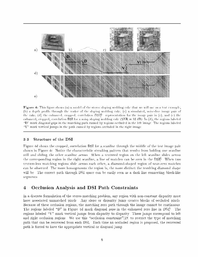
Figure 4: This �gure shows (a) a model of the stereo sloping wedding cake that we will use as a test example,

(b) a depth pro�le through the center of the sloping wedding cake, (c) a simulated, noise-free image pair of

the cake, (d) the enhanced, cropped, correlation DSILi

representation for the image pair in (c), and (e) the

enhanced, cropped, correlation DSI for a noisy sloping wedding cake (SNR = 18 dB). In (d), the regions labeled

\D" mark diagonal gaps in the matching path caused by regions occluded in the left image. The regions labeled

\V" mark vertical jumps in the path caused by regions occluded in the right image.

3.3 Structure of the DSI

Figure 4d shows the cropped, correlation DSI for a scanline through the middle of the test image pair

shown in Figure 4c. Notice the characteristic streaking pattern that results from holding one scanline

still and sliding the other scanline across. When a textured region on the left scanline slides across

the corresponding region in the right scanline, a line of matches can be seen in the DSILi. When two

texture-less matching regions slide across each other, a diamond-shaped region of near-zero matches

can be observed. The more homogeneous the region is, the more distinct the resulting diamond shape

will be. The correct path through DSI space can be easily seen as a dark line connecting block-like

segments.

4 Occlusion Analysis and DSI Path Constraints

In a discrete formulation of the stereo matching problem, any region with non-constant disparity must

have associated unmatched pixels. Any slope or disparity jump creates blocks of occluded pixels.

Because of these occlusion regions, the matching zero path through the image cannot be continuous.

The regions labeled \D" in Figure 4d mark diagonal gaps in the enhanced zero line in DSILi. The

regions labeled \V" mark vertical jumps from disparity to disparity. These jumps correspond to left

and right occlusion regions. We use this \occlusion constraint"[18] to restrict the type of matching

path that can be recovered from each DSIi. Each time an occluded region is proposed, the recovered

path is forced to have the appropriate vertical or diagonal jump.

6

The fact that the disparity path moves linearly through the disparity gaps does not imply that

we presume the a linear interpolation of diparities or a smooth interpolation of depth in the occluded

regions. Rather, the line simply relfects the occlusion constraint that a set of occluded pixels must be

accounted for by a disparity jump of an equal number of pixels.

Nearly all stereo scenes obey the ordering constraint (or monotonicity constraint [18]): if object

a is to the left of object b in the left image then a will be to the left of b in the right image. Thin

objects with large disparities violate this rule, but they are rare in many scenes of interest. Exceptions

to the monotonicity constraint and a proposed technique to handle such cases is given in [16]. By

assuming the ordering rule we can impose a second constraint on the disparity path through the DSI

that signi�cantly reduces the complexity of the path-�nding problem. In the DSILi, moving from left

to right, diagonal jumps can only jump forward (down and across) and vertical jumps can only jump

backwards (up).

It is interesting to consider what happens when the ordering constraint does not hold. Consider

an example of skinny pole or tree signi�cantly in front of a building. Some region of the building

will be seen in the left eye as being to the left of the pole, but in the right eye as to the right of the

pole. If a stereo system is enforcing the ordering constraint it can generate two possible solutions. IN

one case it can ignore the pole completely, considering the pole pixels in the left and right image as

simply noise. More likely, the system will generate a surface the extends sharply forward to the pole

and then back again to the background. The pixels on these two surfaces would actually be the same,

but the system would consider them as unmatched, each surface being occluded from one eye by the

pole. Later, where we decsribe the e�ect of ground control points, we will see how our system chooses

between these solutions.

5 Finding the Best Path

Using the occlusion constraint and ordering constraint, the correct disparity path is highly constrained.

From any location in the DSILi, there are only three directions a path can take { a horizontal match, a

diagonal occlusion, and a vertical occlusion. This observation allows us to develop a stereo algorithm

that integrates matching and occlusion analysis into a single process.

However, the number of allowable paths obeying these two constraints is still huge.3 As noted

by previous researchers [18, 14, 19] one can formulate the task of �nding the best path through the

DSI as a dynamic programming (DP) path-�nding problem in (x; disparity) space. For each scaneline

i, we wish to �nd the minimum cost traversal through the DSIi image which satis�es the occlusion

constraints.

5.1 Dynamic Programming Constraints

DP algorithms require that the decision making process be ordered and that the decision at any state

depend only upon the current state. The occlusion constraint and ordering constraint severely limit

the direction the path can take from the path's current endpoint. If we base the decision of which path

to choose at any pixel only upon the cost of each possible next step in the path and not on any previous

moves we have made, we satisfy the DP requirements and can use DP to �nd the optimal path.

As we traverse through the DSI image constructing the optimal path, we can consider the system

as being in any one of three states: match (M), vertical occlusion (V), or diagonal occlusion (D).

3For example, given a 256 pixel-wide scan-line with a maximum disparity shift of 45 pixels there are 3e+191 possiblelegal paths.

7

M V D

M V DM V D

M V D

Current state &Location

MVD

= Match state= Vertical occlusion= Horizontal occlusion

d j

d j-1

d j+1

x i x i+1

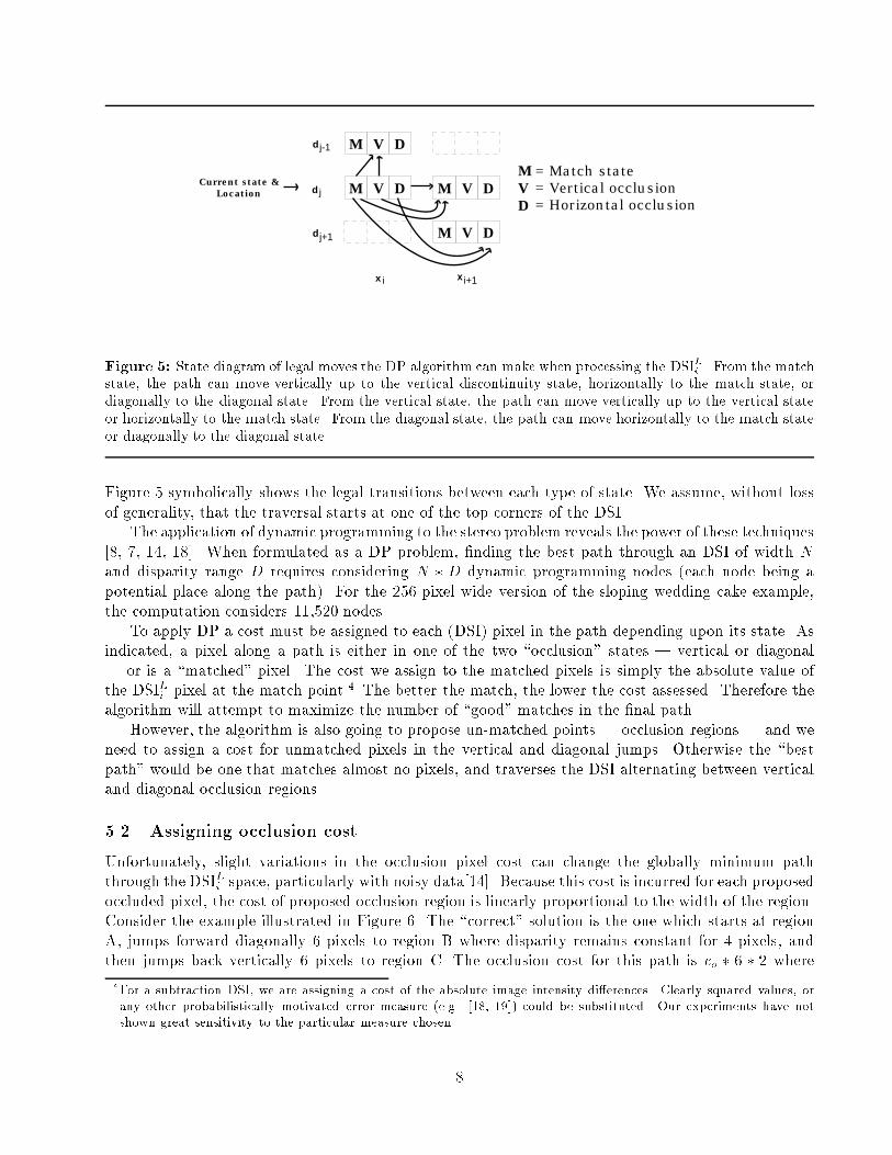
Figure 5: State diagram of legal moves the DP algorithm can make when processing the DSILi. From the match

state, the path can move vertically up to the vertical discontinuity state, horizontally to the match state, or

diagonally to the diagonal state. From the vertical state, the path can move vertically up to the vertical state

or horizontally to the match state. From the diagonal state, the path can move horizontally to the match state

or diagonally to the diagonal state.

Figure 5 symbolically shows the legal transitions between each type of state. We assume, without loss

of generality, that the traversal starts at one of the top corners of the DSI.

The application of dynamic programming to the stereo problem reveals the power of these techniques

[8, 7, 14, 18]. When formulated as a DP problem, �nding the best path through an DSI of width N

and disparity range D requires considering N � D dynamic programming nodes (each node being a

potential place along the path). For the 256 pixel wide version of the sloping wedding cake example,

the computation considers 11,520 nodes.

To apply DP a cost must be assigned to each (DSI) pixel in the path depending upon its state. As

indicated, a pixel along a path is either in one of the two \occlusion" states | vertical or diagonal

| or is a \matched" pixel. The cost we assign to the matched pixels is simply the absolute value of

the DSILipixel at the match point.4 The better the match, the lower the cost assessed. Therefore the

algorithm will attempt to maximize the number of \good" matches in the �nal path.

However, the algorithm is also going to propose un-matched points | occlusion regions | and we

need to assign a cost for unmatched pixels in the vertical and diagonal jumps. Otherwise the \best

path" would be one that matches almost no pixels, and traverses the DSI alternating between vertical

and diagonal occlusion regions.

5.2 Assigning occlusion cost

Unfortunately, slight variations in the occlusion pixel cost can change the globally minimum path

through the DSILispace, particularly with noisy data[14]. Because this cost is incurred for each proposed

occluded pixel, the cost of proposed occlusion region is linearly proportional to the width of the region.

Consider the example illustrated in Figure 6. The \correct" solution is the one which starts at region

A, jumps forward diagonally 6 pixels to region B where disparity remains constant for 4 pixels, and

then jumps back vertically 6 pixels to region C. The occlusion cost for this path is co � 6 � 2 where

4For a subtraction DSI, we are assigning a cost of the absolute image intensity di�erences. Clearly squared values, orany other probabilistically motivated error measure (e.g. [18, 19]) could be substituted. Our experiments have notshown great sensitivity to the particular measure chosen.

8

Desired path

Path chosen if occlusion cost too high

= Occluded Pixel

A

B

C

(light arrow) = Bad matches substituted for occlusion pixels

(bold arrow) = Path selected using good matches and occlusion pixels

Figure 6: The total occlusion cost for an object shifted D pixels can be costocclusion �D �2. If the cost becomes

high, a string of bad matches may be a less expensive path. To eliminate this undesirable e�ect, we must impose

another constraint.

co is the pixel occlusion cost. If the co is too great, a string of bad matches will be selected as the

lower-cost path, as shown. The fact that previous DP solutions to stereo matching (e.g. [19]) present

results where they vary the occlusion cost from one example to the next indicates the sensitivity of

these approaches to this parameter.

In the next section we derive an additional constraint which greatly mitigates the e�ect of the choice

of the occlusion cost co. In fact, all the results of the experiments section use the same occlusion cost

across widely varying imaging conditions.

5.3 Ground control points

In order to overcome this occlusion cost sensitivity, we need to impose another constraint in addition

to the occlusion and ordering constraints. However, unlike previous approaches we do not want to

bias the solution towards any generic property such as smoothness across occlusions[18], inter-scanline

consistency[26, 14], or intra-scanline \goodness"[14].

Instead, we use high con�dence matching guesses: Ground control points (GCPs). These points are

used to force the solution path to make large disparity jumps that might otherwise have been avoided

because of large occlusion costs. The basic idea is that if a few matches on di�erent surfaces can

identi�ed before the DP matching process begins, these points can be used to drive the solution.

Figure 7 illustrates this idea showing two GCPs and a number of possible paths between them. We

note that regardless of the disparity path chosen, the discrete lattice ensures that path-a, path-b, and

path-c all require 6 occlusion pixels. Therefore, all three paths incur the same occlusion cost. Our

algorithm will select the path that minimizes the cost of the proposed matches independent of where

occlusion breaks are proposed and (almost) independent of the occlusion cost value. If there is a single

occlusion region between the GCPs in the original image, the path with the best matches is similar to

path-a or path-b. On the other hand, if the region between the two GCPs is sloping gently, then a

path like path-c, with tiny, interspersed occlusion jumps will be preferred, since it will have the better

matches.5 The path through (x, disparity) space, therefore, will be constrained solely by the occlusion

5There is a problem of semantics when considering sloping regions in a lattice-based matching approach. As is apparentfrom the state diagram in Figure 5 the only depth pro�le that can be represented without occlusion is constant disparity.Therefore a continuous surface which is not fronto-parallel with respect to the camera will be represented by a staircase

9

= Ground Control Point

= Occluded Pixel

Path A

Path B

Path C

Path D

Paths A,B, and C have 6 occludedpixels.

Path D has 14 occluded pixels.

Figure 7: Once a GCP has forced the disparity path through some disparity-shifted region, the occlusion will

be proposed regardless of the cost of the occlusion jump. The path between two GCPs will depend only upon the

good matches in the path, since the occlusion cost is the same for each path A,B, and C. path D is an exception,

since an additional occlusion jump has been proposed. While that path is possible, it is unlikely the globally

optimum path through the space will have any more occlusion jumps than necessary unless the data supporting

a second occlusion jump is strong.

and ordering constraints and the goodness of the matches between the GCPs.

Of course, we are limited to how small the occlusion cost can be. If it is smaller than the typical

value of correct matches (non-zero due to noise)6 then the algorithm proposes additional occlusion

regions such as in path-d of Figure 7. For real stereo images (such as the JISCT test set [9]) the typical

DSI value for incorrectly matched pixels is signi�cantly greater than that of correctly matched ones

and performance of the algorithm is not particularly sensitive to the occlusion cost.

Also, we note that while we have attempted to remove smoothing in uences entirely, there are

situations in which the occlusion cost induces smooth solutions. If no GCP is proposed on a given

surface, and if the stereo solution is required to make a disarity jump across an occlusion region to

reach the correct disparity level for that surface, then if the occlusion cost is high, the preferred solution

will be a at, \smooth" surface. As we will show in some of our results, even scenes with thin surfaces

separated by large occlusion regions tend to give rise to an adequate number of GCPs (the next section

describes our method for selecting such points). This experience is in agreement with results indicating

a substantial percentage of points in a stereo pair can be matched unambiguously, such as Hannah's

\anchor points" [20].

5.4 Why ground control points provide additional constraint

Before proceeding it is important to consider why ground control points provide any additional con-

straint to the dynamic programming solution. Given that they represent excellent matches and there-

fore have very low match costs it is plausible to expect that the lowest cost paths through disparity

space would naturally include these points. While this is typically the case when the number of oc-

clusion pixels is small compared to the number of matched pixels, it is not true in general, and is

of constant disparity regions interspersed with occlusion pixels, even though there are no \occluded" pixels in theordinary sense. In [19] they refer to these occlusions as lattice-induced, and recommend using sub-pixel resolution to�nesse the problem. An alternative would be to use an iterative warping technique as �rst proposed in [27].

6Actually, it only has to be greater than half the typical value of the correct matches. This is because each diagonalpixel jumping forward must have a corresponding vertical jump back to end up at the same GCP.

10

= GCP = Occluded Pixel= Multi-valued GCP

Path A Path B Path C

= Prohibited Pixel

Figure 8: The use of multiple GCPs per column. Each path through the two outside GCPs have exactly the

same occlusion cost, 6co. As long as the path passes through one of the 3 multi-GCPs in the middle column it

avoids the (in�nite) penalty of the prohibited pixels.

particularly problematic in situations with large disparity regions.

Consider again Figure 6. Let us assume that region B represents perfect matches and therefore

has a match cost of zero. These are the types of points which will normally be selected as GCPs (as

described in the next section). Whether the minimal cost path from A to C will go through region

B is dependent upon the relative magnitude between the occlusion cost incurred via the diagonal and

vertical jumps required to get to region B and the incorrect match costs of the horizontal path from

A to C. It is precisely this sensitivity to the occlusion cost that has forced previous approaches to

dynamic programming solutions to enforce a smoothness constraint.

5.5 Selecting and enforcing GCPs

If we force the disparity path through GCPs, their selection must be highly reliable. We use several

heuristic �lters to identify GCPs before we begin the DP processing; several of these are similar to

those used by Hannah [20] to �nd highly reliable matches. The �rst heuristic requires that a control

point be both the best left-to-right and best right-to-left match. In the DSI approach these points are

easy to detect since such points are those which are the best match in both their diagonal and vertical

columns. Second, to avoid spurious \good" matches in occlusion regions, we also require that a control

point have match value that is smaller than the occlusion cost. Third, we require su�cient texture

in the GCP region to eliminate homogenous patches that match a disparity range. Finally, to further

reduce the likelihood of a spurious match, we exclude any proposed GCPs that have no immediate

neighbors that are also marked as GCPs.

Once we have a set of control points, we force our DP algorithm to choose a path through the

points by assigning zero cost for matching with a control point and a very large cost to every other

path through the control point's column. In the DSILi, the path must pass through each column at

some pixel in some state. By assigning a large cost to all paths and states in a column other than a

match at the control point, we have guaranteed that the path will pass through the point.

An important feature of this method of incorporating GCPs is that it allows us to have more than

one GCP per column. Instead of forcing the path through one GCP, we force the path through one of

a few GCPs in a column as illustrated in Figure 8. Even if using multiple windows and left-to-right,

right-to-left matching, it is still possible that we will label a GCP in error if only one GCP per column

is permitted. It is unlikely, however, that none of several proposed GCPs in a column will be the

correct GCP. By allowing multiple GCPs per column, we have eliminated the risk of forcing the path

through a point erroneously marked as high-con�dence due image noise without increasing complexity

or weakening the GCP constraint. This technique also alows us to handle the \wallpaper" problem of

11

GCP 1

= Legal Area = Excluded Area = Ground Control Point

GCP2

D

Figure 9: GCP constraint regions. Each GCP removes a pair of similar triangles from the possible solution

path. If the GCP is at one extreme of the disparity range (GCP 1), then the area excluded is maximized at

D2=2. If the GCP is exactly in the middle of the disparity range (GCP 2) the areas is minimized at D2=4.

matching in the presence of a repeated pattern in the scene: multiple GCPs allow the elements of the

pattern to repeatedly matched (locally) with high con�dence while ensuring a global minimum.

5.6 Reducing complexity

Without GCPs, the DP algorithm must consider one node for every point in the DSI, except for the

boundary conditions near the edges. Speci�cation of a GCP, however, essentially introduces an in-

tervening boundary point and prevents the solution path from traversing certain regions of the DSI.

Because of the occlusion and monotonicity constraints, each GCP carves out two complimentary tri-

angles in the DSI that are now not valid. Figure 9 illustrates such pairs of triangles. The total area

of the two triangles, A, depends upon at what disparity d the GCP is located, but is known to lie

within the range D2=4 � A � D2=2 where D is the allowed disparity range. For the 256 pixel wedding

cake image, 506 � A � 1012. Since the total number of DP nodes for that image is 11,520 each GCP

whose constraint triangles do not overlap with another pair of GCP constraint triangles reduces the DP

complexity by about 10%. With several GCPs the complexity is less than 25% of the original problem.

6 Results using GCPs

Input to our algorithm consists of a stereo pair. Epipolar lines are assumed to be known and corrected

to correspond to horizontal scanlines. We assume that additive and multiplicative photometric bias

between the left and right images is minimized allowing the use of a substraction DSI for matching. As

mentioned, such baises can be handled by using the appropriate correlation operator. The birch tree

example shows that the subtraction DSI performs well even with signi�cant additive di�erences.

The dynamic programming portion of our algorithm is quite fast; almost all time was spent in

creating the correlation DSI used for �nding GCPs. Generation time for each scanline depends upon

the e�ciency of the correlation code, the number and size of the masks, and the size of the original

imagery. Running on a HP 730 workstation with a 515x512 image using nine 7x7 �lters and a maximum

disparity shift of 100 pixels, our current implementation takes a few seconds per scanline. However, since

the most time consuming operations are simple window-based cross-correlation, the entire procedure

could be made to run near real time with simple dedicated hardware. Furthermore, this step was used

solely to provide GCPs; a faster high con�dence match detector would eliminate most of this overhead.

12

a) b)

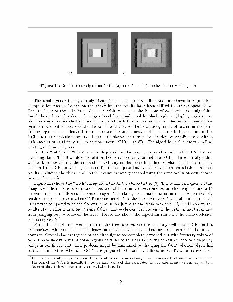
Figure 10: Results of our algorithm for the (a) noise-free and (b) noisy sloping wedding cake.

The results generated by our algorithm for the noise-free wedding cake are shown in Figure 10a.

Computation was performed on the DSILibut the results have been shifted to the cyclopean view.

The top layer of the cake has a disparity with respect to the bottom of 84 pixels. Our algorithm

found the occlusion breaks at the edge of each layer, indicated by black regions. Sloping regions have

been recovered as matched regions interspersed with tiny occlusion jumps. Because of homogenous

regions many paths have exactly the same total cost so the exact assignment of occlusion pixels in

sloping regions is not identical from one scane line to the next, and is sensitive to the position of the

GCPs in that particular scanline. Figure 10b shows the results for the sloping wedding cake with a

high amount of arti�cially generated noise noise (SNR = 18 dB). The algorithm still performs well at

locating occlusion regions.

For the \kids" and \birch" results displayed in this paper, we used a subtraction DSI for our

matching data. The 9-window correlation DSI was used only to �nd the GCPs. Since our algorithm

will work properly using the subtraction DSI, any method that �nds highly-reliable matches could be

used to �nd GCPs, obviating the need for the computationally expensive cross correlation. All our

results, including the \kids" and \birch" examples were generated using the same occlusion cost, chosen

by experimentation.

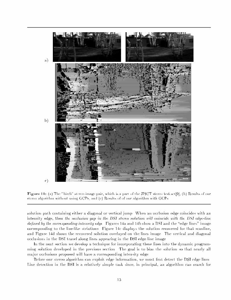
Figure 11a shows the \birch" image from the JISCT stereo test set[9]. The occlusion regions in this

image are di�cult to recover properly because of the skinny trees, some texture-less regions, and a 15

percent brightness di�erence between images. The skinny trees make occlusion recovery particularly

sensitive to occlusion cost when GCPs are not used, since there are relatively few good matches on each

skinny tree compared with the size of the occlusion jumps to and from each tree. Figure 11b shows the

results of our algorithm without using GCPs. The occlusion cost prevented the path on most scanlines

from jumping out to some of the trees. Figure 11c shows the algorithm run with the same occlusion

cost using GCPs.7

Most of the occlusion regions around the trees are recovered reasonably well since GCPs on the

tree surfaces eliminated the dependence on the occlusion cost. There are some errors in the image,

however. Several shadow regions of the birch �gure are completely washed-out with intensity values of

zero. Consequently, some of these regions have led to spurious GCPs which caused incorrect disparity

jumps in our �nal result. This problem might be minimized by changing the GCP selection algorithm

to check for texture wherever GCPs are proposed. On some scanlines, no GCPs were recovered on

7The exact value of co depends upon the range of intensities in an image. For a 256 grey level image we use co = 12:The goal of the GCPs is insensitivity to the exact value of this parameter. In our experiments we can vary co by afactor of almost three before seeing any variation in reults.

13

some trees which led to the scanline gaps in some of the trees.

Note the large occlusion regions generated byd the third tree from the left. This example of small

foreground object generating a large occlusion region is a violation of the ordering contraint. As

decsribed previously, if the DP solution includes the trees it cannot also include the common region

of the building. If there are GCPs on both the building and the trees, only one set of GCPs can be

accomodated. Because of the details of how we incorporated GCPs into the DP algorithm, the surface

with the greater number will dominate. In the tree example, the grass regions were highly shadowed

and typically did not generate many GCPs.8

Figure 12a is an enlarged version of the left image of Figure 1. Figure 12b shows the results obtained

by the algorithm developed by Cox et al.[14]. The Cox algorithm is a similar DP procedure which uses

inter-scanline consistency instead of GCPs to reduce sensitivity to occlusion cost.

Figure 12c shows our results on the same image. These images have not been converted to the

cyclopean view, so black regions indicate regions occluded in the left image. The Cox algorithm does

a reasonably good job at �nding the major occlusion regions, although many rather large, spurious

occlusion regions are proposed.

When the algorithm generates errors, the errors are more likely to propagate over adjacent lines,

since inter-and intra-scanline consistency are used[14]. To be able to �nd the numerous occlusions,

the Cox algorithm requires a relatively low occlusion cost, resulting in false occlusions. Our higher

occlusion cost and use of GCPs �nds the major occlusion regions cleanly. For example, the man's head

is clearly recovered by our approach. The algorithm did not recover the occlusion created by the man's

leg as well as hoped since it found no good control points on the bland wall between the legs. The wall

behind the man was picked up well by our algorithm, and the structure of the people in the scene is

quite good. Most importantly, we did not use any smoothness or inter- and intra-scanline consistencies

to generate these results.

We should note that our algorithm does not perform as well on images that only have short match

regions interspersed with many disparity jumps. In such imagery our conservative method for selecting

GCPs fails to provide enough constraint to recover the proper surface. However, the results on the

birch imagery illustrate that in real imagery with many occlusion jumps, there are likely to be enough

stable regions to drive the computation.

7 Edges in the DSI

Figure 13 displays the DSILi

for a scanline from the man and kids stereo pair in Figure 12; this

particular scanline runs through the man's chest. Both vertical and diagonal striations are visible in

the DSI data structure. These line-like striations are formed wherever a large change in intensity (i.e.

an \edge") occurs in the left or right scan line. In the DSILithe vertical striations correspond to

large changes in intensity in IL and the diagonal striations correspond to changes in IR. Since the

interior regions of objects tend to have less intensity variation than the edges, the subtraction of an

interior region of one line from an intensity edge of the other tends to leave the edge structure in tact.

The persistence of the edge traces a linear structure in the DSI. We refer to the lines in the DSI as

\edge-lines."

As mentioned in the introduction, occlusion boundaries tend to induce discontinuities in image

intensity, resulting in intensity edges. Recall that an occlusion is represented in the DSI by the stereo

8In fact the birch tree example is a highly pathological case because of the unbalanced dynamic range of the two images.For example while 23% of the pixels in the left image have an intensity value of 0 or 255, only 6% of the pixels in theright image were similarly clipped. Such extreme clipping limited the ability of the GCP �nder to �nd unambiguousmatches in these regions.

14

a)

b)

c)

Figure 11: (a) The "birch" stereo image pair, which is a part of the JISCT stereo test set[9], (b) Results of our

stereo algorithm without using GCPs, and (c) Results of of our algorithm with GCPs.

solution path containing either a diagonal or vertical jump. When an occlusion edge coincides with an

intensity edge, then the occlusion gap in the DSI stereo solution will coincide with the DSI edge-line

de�ned by the corresponding intensity edge. Figures 14a and 14b show a DSI and the \edge-lines" image

corresponding to the line-like striations. Figure 14c displays the solution recovered for that scanline,

and Figure 14d shows the recovered solution overlayed on the lines image. The vertical and diagonal

occlusions in the DSI travel along lines appearing in the DSI edge-line image.

In the next section we develop a technique for incorporating these lines into the dynamic program-

ming solution developed in the previous section. The goal is to bias the solution so that nearly all

major occlusions proposed will have a corresponding intensity edge.

Before our stereo algorithm can exploit edge information, we must �rst detect the DSI edge-lines.

Line detection in the DSI is a relatively simple task since, in principal, an algorithm can search for

15

a)

b)

c)

Figure 12: Results of two stereo algorithms on Figure 1. (a) Original left image. (b) Cox et al. algorithm[14],

and (c) the algorithm described in this paper.

diagonal and vertical lines only. For our initial experiments, we implemented such an edge �nder.

However, the computational ine�ciencies of �nding edges in the DSI for every scan line led us to seek

a one pass edge detection algorithm that would approximate the explicit search for lines in every DSI.

Our heuristic is to use a standard edge-�nding procedure on each image of the original image pair

and use the recovered edges to generate an edge-lines image for each DSI. We have used a simpli�ed

Canny edge detector to �nd possible edges in the left and right image[10] and combined the vertical

components of those edges to recover the edge-lines.

The use of a standard edge operator introduces a constraint into the stereo solution that we pur-

posefully excluded until now: inter-scanline consistency. Because any spatial operator will tend to �nd

coherent edges, the result of processing one scanline will no longer be independent of its neighboring

scanlines. However, since the inter-scanline consistency is only encouraged with respect to edges and

occlusion, we are willing to include this bias in return for the computationally e�ciency of single pass

edge detection.

16

Figure 13: A subtraction DSILi

for the imagery of Figure 12, where i is a scanline through the man's chest.

Notice the diagonal and vertical striations that form in the DSILi due to the intensity changes in the image pair.

These edge-lines appear at the edges of occlusion regions.

a)

b)

c)

d)

Figure 14: (a) A cropped, subtraction DSILi. (b) The lines corresponding to the line-like striations in (a). (c)

The recovered path. (d) The path and the image from (b) overlayed. The paths along occlusions correspond to

the paths along lines.

17

Ground Control Point (GCP)

Line in lines DSI

Ideal path

Other possible paths

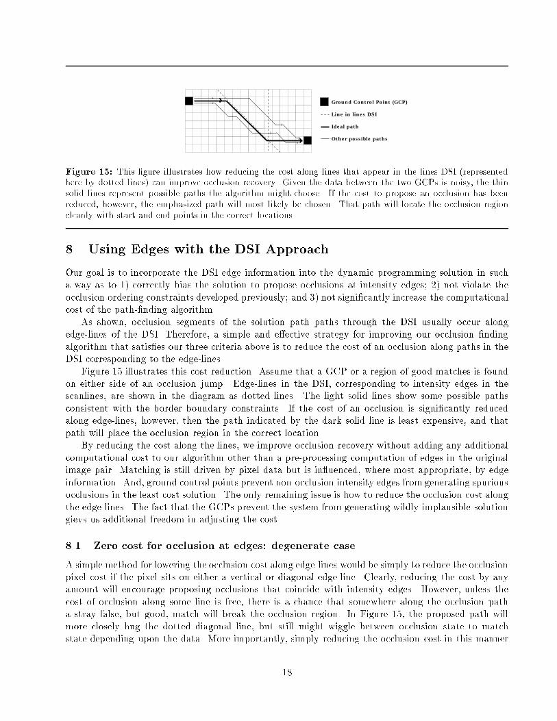
Figure 15: This �gure illustrates how reducing the cost along lines that appear in the lines DSI (represented

here by dotted lines) can improve occlusion recovery. Given the data between the two GCPs is noisy, the thin

solid lines represent possible paths the algorithm might choose. If the cost to propose an occlusion has been

reduced, however, the emphasized path will most likely be chosen. That path will locate the occlusion region

cleanly with start and end points in the correct locations.

8 Using Edges with the DSI Approach

Our goal is to incorporate the DSI edge information into the dynamic programming solution in such

a way as to 1) correctly bias the solution to propose occlusions at intensity edges; 2) not violate the

occlusion ordering constraints developed previously; and 3) not signi�cantly increase the computational

cost of the path-�nding algorithm.

As shown, occlusion segments of the solution path paths through the DSI usually occur along

edge-lines of the DSI. Therefore, a simple and e�ective strategy for improving our occlusion �nding

algorithm that satis�es our three criteria above is to reduce the cost of an occlusion along paths in the

DSI corresponding to the edge-lines.

Figure 15 illustrates this cost reduction. Assume that a GCP or a region of good matches is found

on either side of an occlusion jump. Edge-lines in the DSI, corresponding to intensity edges in the

scanlines, are shown in the diagram as dotted lines. The light solid lines show some possible paths

consistent with the border boundary constraints. If the cost of an occlusion is signi�cantly reduced

along edge-lines, however, then the path indicated by the dark solid line is least expensive, and that

path will place the occlusion region in the correct location.

By reducing the cost along the lines, we improve occlusion recovery without adding any additional

computational cost to our algorithm other than a pre-processing computation of edges in the original

image pair. Matching is still driven by pixel data but is in uenced, where most appropriate, by edge

information. And, ground control points prevent non-occlusion intensity edges from generating spurious

occlusions in the least cost solution. The only remaining issue is how to reduce the occlusion cost along

the edge-lines. The fact that the GCPs prevent the system from generating wildly implausible solution

gievs us additional freedom in adjusting the cost.

8.1 Zero cost for occlusion at edges: degenerate case

A simple method for lowering the occlusion cost along edge-lines would be simply to reduce the occlusion

pixel cost if the pixel sits on either a vertical or diagonal edge-line. Clearly, reducing the cost by any

amount will encourage proposing occlusions that coincide with intensity edges. However, unless the

cost of occlusion along some line is free, there is a chance that somewhere along the occlusion path

a stray false, but good, match will break the occlusion region. In Figure 15, the proposed path will

more closely hug the dotted diagonal line, but still might wiggle between occlusion state to match

state depending upon the data. More importantly, simply reducing the occlusion cost in this manner

18

Proposed Match

Proposed Occlusion

Lines (from edges)

L R

(a) (b)

Figure 16: (a) When the occlusion cost along both vertical and diagonal edge-lines is set to zero, the recovered

path will maximize the number of proposed occlusions and minimize the number of matches. Although real

solutions of this nature do exist, an example of which is shown in (b), making both vertical and diagonal

occlusion costs free generates these solutions even when enough matching data exists to support a more likely

result.

re-introduces a sensitivity to the value of that cost; the goal of the GCPs was the elimination of that

sensitivity.

If the dotted path in Figure 15 were free, however, spurious good matches would not a�ect the

recovered occlusion region. An algorithm can be de�ned in which any vertical or diagonal occlusion

jump corresponding to an edge-line has zero cost. This method would certainly encourage occlusions

to be proposed along the lines.

Unfortunately, this method is a degenerate case. The DP algorithm will �nd a solution that

maximizes the number of occlusion jumps through the DSI and minimizes the number of matches,

regardless of how good the matches may be. Figure 16a illustrates how a zero cost for both vertical

and diagonal occlusion jumps leads to nearly no matches begin proposed. Figure 16b shows that this

degenerate case does correspond to a potentially real camera and object con�guration. The algorithm

has proposed a feasible solution. The problem, however, is that the algorithm is ignoring huge amounts

of well-matched data by proposing occlusion everywhere.

8.2 Focusing on occlusion regions

In the previous section we demonstrated that one cannot allow the traversal of both diagonal and

vertical lines in the DSI to be cost free. Also, a compromise of simply lowering the occlusion cost along

both types of edges re-introduces dependencies on that cost. Because one of the goals of our approach is

the recovery of the occlusion regions, we choose to make the diagonal occlusion segments free, while the

vertical segments maintain the normal occlusion pixel cost. The expected result is that the occlusion

regions corresponding to the diagonal gaps in the DSI should be nicely delineated while the occlusion

edges (the vertical jumps) are not changed. Furthermore, we expect no increased sensitivity to the

occlusion cost.9

9The alternative choice of making the vertical segments free might be desired in the case of extensive limb edges. Assumethe system is viewing a sharply rounded surface (e.g. a telephone pole) in front of some other surface, and considerthe image from the left eye. Interiror to left edge of the pole as seen in the left eye are some pole pixels that are notviewed by the right eye. From a stereo matching perspective, these pixels are identical to the other occlusion pixelsvisible in the left but not right eyes. However, the edge is in the wrong place if focusing on the occlusion regions, e.g.the diagonal disparity jumps in the left image for the left side of the pole. In the right eye, the edge is at the correctplace and could be used to bias the occulsion recovery. Using the right eye to establish the edges for a left occlusionregion (visible only in the left eye) and visa versa, is accomplished by biasing the vertical lines in the DSI. Because wedo not have imagery wth signi�cant limb boundaries we have not experimented with this choice of bias.

19

(a)

(c)

(b)

(d)

Figure 17: (a) Synthetic trees left image, (b) occlusion result without GCPs or edge-lines, (c) occlusion result

with GCPs only, and (d) result with GCPs and edge-lines.

Figure 17a shows a synthetic stereo pair from the JISCT test set[9] of some trees and rocks in a �eld.

Figure 17b shows the occlusion regions recovered by our algorithm when line information and GCP

information is not used, comparable to previous approaches (e.g. [14]). The black occlusion regions

around the trees and rocks are usually found, but the boundaries of the regions are not well de�ned and

some major errors exist. Figure 17c displays the results of using only GCPs, with no edge information

included. The dramatic improvement again illustrates the power of the GCP constraint. Figure 17d

shows the result when both GCPs and edges have been used. Though the improvement over GCPs

alone is not nearly as dramatic, the solution is better. For example, the streaking at the left edge of the

crown of the rightmost tree has been reduced. In general, the occlusion regions have been recovered

almost perfectly, with little or no streaking or false matches within them. Although the overall e�ect

of using the edges is small, it is important in that it biases the occlusion discontinuities to be proposed

in exactly the right place.

20

9 Non-cyclopean Views: Stereo Layers

Occlusion regions can be used to label object boundaries and layers of objects in a scene. For many, if

not most, applications qualitative information that segments the scene into layers is more useful than

precise, quantitative depth measurement. Object segmentation, motion analysis, object recognition,

and image coding algorithms would all bene�t from depth layering that preserves sharp `silouhette"

discontinuity boundaries[30].

Most previous work on detecting depth discontinuities in stereo (e.g. [17]) proposes some operation

on the recovered depth map. For example, Terzopolous proposed a thin-metal plate interpolation

technique[29] and fracturing the plate at areas of high strain. But a much more direct method of

detecting the depth discontinuities is to make explicit use of the discovered occlusion regions.

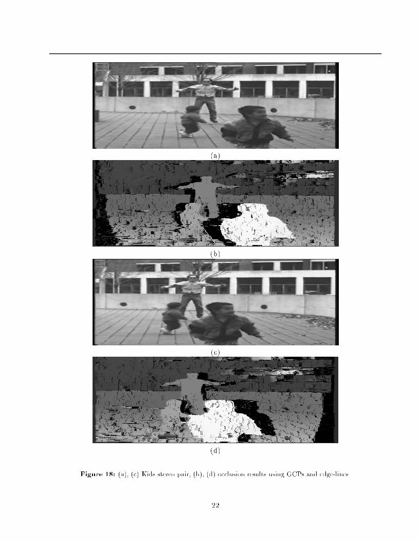
Figures 18a and 18c are a stereo pair from a sequence of a man and two kids; this type of imagery

has very large occlusion regions. For most computer vision applications such as tracking or modeling,

segmentation of the man's arms and legs is more valuable information than the exact leg curvature.

The outline shape of the man and his layered position with respect to the other objects in the scene

(the background and two kids) is critical information that can be provided reliably by stereo algorithms

that include occlusion analysis.

Our method uses edge information asymmetrically, concentrating on recovering the occlusion regions

(as opposed to edges) in each image of the stereo pair. Thus, our algorithm generates two occlusion

maps, one optimized to �nd each type of occlusion. Figures 18b and 18d show the stereo disparities

and occlusion regions recovered using the DSILiand the DSIR

i, respectively. Studying the left and

right occlusion regions in these �gures, the advantage of using a dual-image solution becomes clear. In

the left result (18c), the left occlusion regions are generally correct, but the right occlusion edges still

have a \ragged" quality, like at the right edge of the man's left leg (marked as region A). In the dual,

right solution (18d), however, the right occlusion region of the same leg is recovered more precisely

(marked as region B). Other parts of the occlusion recovery are also improved using dual solutions,

such as the left edge of the rightmost kids's head. The right occlusion result recovers a \ragged" left

occlusion edge (marked as region C), but the left occlusion result �nds the left occlusion region and

the boundary of the kids's head more cleanly (marked as region D). Instead of generating a single,

mediocre, cyclopean reconstruction by reducing the occlusion cost by half for occlusion regions and

occlusion edges, we produce two: one with better left occlusion regions and the other with better right

occlusion regions.

We have just begun to explore the idea of stereo layers and have not yet constructed methods for

using the occlusion maps to de�ne the layers. Also, because the idea of layers becomes particularly

useful when considering image sequences[30] we will need to consider any interaction between layers

de�ned by motion and those de�ned by stereo.

10 Conclusion

10.1 Summary

We have presented a stereo algorithm that incorporates the detection of occlusion regions directly

into the matching process, yet does not use smoothness or intra- or inter-scanline consistency criteria.

Employing a dynamic programming solution that obeys the occlusion and ordering constraints to �nd

a best path through the disparity space image, we eliminate sensitivity to the occlusion cost by the

use of ground control points (GCPs)| high con�dence matches. These points improve results, reduce

complexity, and minimize dependence on occlusion cost without arbitrarily restricting the recovered

21

(a)

A D

(b)

(c)

CB

(d)

Figure 18: (a), (c) Kids stereo pair, (b), (d) occlusion results using GCPs and edge-lines.

22

solution. Finally, we extend the technique to exploit the relationship between occlusion jumps and

intensity edges. Our methd is to reduce the cost of proposed occlusion edges that coincide with

intensity edges. The result is an algorithm that extracts large occlusion regions accurately without

requiring external smoothness criteria.

10.2 Relation to psychophysics

As mentioned at the outset, there is considerable psychophysical evidence that occlusion regions �gure

somewhat prominently in the human perception of depth from stereo (e.g. [28, 25]). And, it has become

common (e.g. [19]) to cite such evidence in support of computational theories of stereo matching that

explicitly model occlusion.

However, for the approach we have presented here we believe such reference would be a bit disin-

genuous. Dynamic programming is a powerful tool for a serial machine attacking a locally decided,

global optimization problem. But given the massively parallel computations performed by the human

vision system, it seems unlikely that such an approach is particularly relevant to understanding human

capabilities.

However, we note that the two novel ideas of this paper | the use of ground control points to drive

the stereo solution in the presence of occlusion, and the integration of intensity edges into the recovery

of occlusion regions | are of interest to those considering human vision.

One way of interpreting ground control points is as unambiguous matches that drive the resulting

solution such that points whose matches are more ambiguous will be correctly mapped. The algorithm

presented in this paper has been constructed so that relatively few GCPs (one per surface plane) are

needed to result in an entirely unambiguous solution. This result is consistent with the \pulling e�ect"

reported in the psychophysical literature (e.g. [22]) in which very few unambiguous \bias" dots (as

little as 2%) are needed to pull an ambiguous stereogram to the depth plane of the unambiguous

points. Although several interpretations of this e�ect are possible (e.g. see [1]) we simply note that it

is consistent with the idea of a few cleanly matched points driving the solution.

Second, there has been recent work [1] demonstrating the importance of edges in the perception

of occlusion. Besides providing some wonderful demonstrations of the impact of intensity edges in

the perception of occlusion, they also develop a receptive-�eld theory of occlusion detection. Their

receptive �elds require a vertical decorrelation edge where on one side of the edge the images are

correlated (matched), while on the other they are not. Furthermore, they �nd evidence that the

strength the edge directly a�ects the stability of the perception of occlusion. Though the mechanism

they propose is quite di�erent than those discussed here, this is the �rst strong evidence we have seen

supporting the importance of edges in the perception of occlusion. Our interpretation is that the human

visual system is exploiting the occlusion edge constraint developed here: occlusion edges usually fall

along intensity edges.

10.3 Open questions

Finally we mention a few open questions that should be addressed if the work presented here is to be

further developed or applied. The �rst involves the recovery of the GCPs. As indicated, having a well

distributed set of control points mostly eliminates the sensitivity ofthe algorithm to the occlsuion cost,

and reduces the computational complexity of the dense match. Our initial experiments using a robust

estimator similar to [20] have been successful, but we feel that a robust estimator explicitly designed

to provide GCPs could be more e�ective.

Second, we are not satis�ed with the awkward manner in which lattice matching techniques | no

subpixel matches and every pixel is either matched or occluded | handle sloping regions. While a

23

staircase of macthed and occluded pixels is to be expected (mathematically) whenever a surface is not

parallel to the image plane, its presence re ects the inability of the lattice to match a region of one

image to a di�erently-sized region in the other. [7] suggests using super resolution to achieve subpixel

matches. While this approach will allow for smoother changes in depth, and should help with matching

by reducing aliasing, it does not really address the issue of non-constant disparity. As we suggested

here, one could apply an iterative warping technique as in [27], but the computational cost may be

excessive.

Finally, there is the problem of order constraint violations as in some of the birch tree examples.

Because of the dynamic programming formulation we use, we cannot incorporate these exceptions,

except perhaps in a post hoc analysis that notices that sharp occluding surfaces actually match. Because

our main emphasis is on demonstrating the e�ectiveness of GCPs we have not energetically explored

this problem.

References

[1] B. Anderson and K. Nakayama. Toward a general theory of stereopsis: Binocular matching,

occluding contour, and fusion. Psychological Review, 101(3):414{445, 1995.

[2] H.H. Baker and T.O. Binford. Depth from edge and intensity based stereo. In Proc. 7th Int. Joint

Conf. Art. Intel., pages 631{636, 1981.

[3] H.H. Baker, R.C. Bolles, and J. Wood�ll. Realtime stereo and motion integration for navigation.

In Proc. Image Understanding Workshop, pages 1295{1304, 1994.

[4] F. Barnard. Computational stereo. Computing Surveys, 14:553{572, 1982.

[5] P. Belhumeur. Bayesian models for reconstructing the scene geometry in a pair of stereo images.

In Proc. Info. Sciences Conf., Johns Hopkins University, 1993.

[6] P. Belhumeur. A binocular stereo algorithm for reconstructing sloping, creased, and broken surfaces

in the presence of half-occlusion. In Proc. Int. Conf. Comp. Vis., 1993.

[7] P. Belhumeur and D. Mumford. A bayseian treatment of the stereo correspondence problem using

half-occluded regions. In Proc. Comp. Vis. and Pattern Rec., 1992.

[8] R.E. Bellman. Dynamic Programming. Princeton University Press, 1957.

[9] R. Bolles, H. Baker, and M. Hannah. The JISCT stereo evaluation. In Proc. Image Understanding

Workshop, pages 263{274, 1993.

[10] J. Canny. A computational approach to edge detection. IEEE Trans. Patt. Analy. and Mach.

Intell., 8(6):679{698, 1986.

[11] C. Chang, S. Catterjee, and P.R. Kube. On an analysis of static occlusion in stereo vision. In

Proc. Comp. Vis. and Pattern Rec., pages 722{723, 1991.

[12] R. Chung, , and R. Nevatia. Use of monocular groupings and occlusion analysis in a hierarchical

stereo system. In Proc. Comp. Vis. and Pattern Rec., pages 50{55, 1991.

[13] S.D. Cochran and G. Medioni. 3-d surface description from binocular stereo. IEEE Trans. Patt.

Analy. and Mach. Intell., 14(10):981{994, 1992.

24

[14] I.J. Cox, S. Hingorani, S.Rao, and B. Maggs. A maximum likelihood stereo algorithm. Comp.

Vis. and Img. Und., 63(3):542{568, 1996.

[15] U.R. Dhond and J.K. Aggarwal. Structure from stereo { a review. IEEE Trans. Sys., Man and

Cyber., 19(6):1489{1510, 1989.

[16] U.R. Dhond and J.K. Aggarwal. Stero matching in the presence of narrow occluding objects using

dynamic disparity search. IEEE Trans. Patt. Analy. and Mach. Intell., 17(7):719{724, 1995.

[17] P. Fua. Combining stereo and monocular information to compute dense depth maps that preserve

depth discontinuities. In Proc. Int. Joint Conf. Art. Intel., pages 1292{1298, 1991.

[18] D. Geiger, B. Ladendorf, and A. Yuille. Occlusions and binocular stereo. In Proc. European Conf.

Comp. Vis., pages 425{433, 1992.

[19] D. Geiger, B. Ladendorf, and A.L. Yuille. Occlusions and binocular stereo. Int. J. of Comp. Vis.,

14(3):211{226, 1995.

[20] M.J. Hannah. A system for digital stereo image matching. Photogrammetric Eng. and Remote

Sensing, 55(12):1765{1770, 1989.

[21] S.S. Intille and A.F. Bobick. Disparity-space images and large occlusion stereo. In Proc. European

Conf. Comp. Vis., pages 179{186, Stockholm, 1994.

[22] B. Julesz and J. Chang. Interaction between pools of binocular disparity detectors tuned to

di�erent disparities. Biological Cybernetics, 22:107{119, 1976.

[23] T. Kanade and M. Okutomi. A stereo matching algorithm with an adaptive window: theory and

experiment. In Proc. Image Understanding Workshop, pages 383{389, 1990.

[24] J.J. Little and W.E. Gillett. Direct evidence for occlusion in stereo and motion. Image and Vision

Comp., 8(4):328{340, 1990.

[25] K. Nakayama and S. Shimojo. Da Vinci stereopsis: depth and subjective occluding contours from

unpaired image points. Vision Research, 30(11):1811{1825, 1990.

[26] Y. Ohta and T. Kanade. Stereo by intra- and inter-scanline search using dynamic programming.

IEEE Trans. Patt. Analy. and Mach. Intell., 7:139{154, 1985.

[27] L.H. Quam. Hierachical warp stereo. In Proc. Image Understanding Workshop, pages 149{155,

New Orleans, LA, 1984.

[28] S. Shimojo and K. Nakayama. Real world occlusion constraints and binocular rivalry. Vision

Research, 30(1):69{80, 1990.

[29] D. Terzopoulos. Regularization of inverse problems involving discontinuities. IEEE Trans. Patt.

Analy. and Mach. Intell., 8(4):413{424, 1986.

[30] J.Y.A. Wang and E.H. Adelson. Layered representation for motion analysis. In Proc. Comp. Vis.

and Pattern Rec., pages 361{366, New York City, June 1993.

[31] Y. Yang, A. Yuille, and J. Lu. Local, global, and multilevel stereo matching. In Proc. Comp. Vis.

and Pattern Rec., 1993.

25