LARGE EDDY SIMULATION IN PEBBLE BED GAS COOLED CORE REACTORS

Yassin A. Hassan Texas A&M University, Texas, USA

Abstract

A High Temperature Gas-cooled Reactor (HTGR) is one of the renewed reactor designs to play a role in nuclear power generation. This reactor design concept is currently under consideration and development worldwide. The combination of coated particle fuel, inert helium gas as coolant and graphite moderated reactor makes possible to operate at high temperature yielding a high efficiency. In this study the simulation of turbulent transport for the gas through the gaps of the spherical fuel elements (fuel pebbles) was performed using the large eddy simulation. This would help in understanding the highly three-dimensional, complex flow phenomena caused by flow curvature in the pebble bed. Resolving all the scales of a turbulent flow is too costly, while employing highly empirical turbulence models to complex problems could give inaccurate simulation results. The large eddy simulation (LES) method would overcome these shortcomings. An attempt to obtain experimental velocity flow patterns using particle image velocimetry technique combined with matched refractive index liquid was pursued.

Introduction

The Generation IV International Forum findings relative to the future nuclear systems (sustainability, security and reliability, economy, non-proliferation and physical protection) have given new impetus to graphite-moderated high-temperature gas cooled reactors (HTGRs). The high modular HTGR concept exhibits inherent safety features due to the low power density and the large amount of graphite present in the core which gives a large thermal inertia in the event of accidents as loss of coolant. These passive concepts were first introduced in German HTR-Module (pebble fuel) design [1, 2]. The fuel design of fissile kernels coated with carbon and silicon carbide layers mixed with graphite is suitable for reaching very high burnup and ensures a full confinement of volatile fission products during normal and abnormal situations. Other characteristics of HTGR are the capability of providing high temperature heat and suitability for various power conversion cycles.

In pebble bed reactor cores, the gas flows around randomly distributed spheres. The understanding of such complex unsteady flows is important. This requires a variety of analysis techniques and simulation tools. These range from simple one-dimensional models [3] that do not capture all the significant physical phenomena to large scale three dimensional computational fluid dynamics (CFD) codes [4]. A huge number of grids is needed to resolve the flow structure around the spheres that require huge CPU time and memory. Unfortunately, there are only few studies [5] which represent a similar flow around randomly distributed spheres as in Pebble Bed Modular Reactors (PBMR) under high Reynolds number flow conditions. Furthermore, most of the turbulence models

331

that were used for these simulations are eddy viscosity models which does not resolve the flow field appropriately where curved flows exist.

Heat transfer in both laminar and turbulent flows varies noticeably around curved surfaces.

Curved flows would be present in the presence of contiguous curved surfaces. In laminar flow condition and appreciable effect of thermo gravitational forces, the Nusselt (Nu) number depends significantly on the curvature shape of the surface. It changes with order of 10 times. The flow passages through the gap between the fuel balls have concave and convex configurations. The action of the centrifugal forces manifests itself differently on convex and concave parts of the flow path (suppression or stimulation of turbulence). This type of flow has distinctive features. In such flows, there is a pressure gradient, which strongly affects the boundary layer behavior. The transition from a laminar to turbulent flow around this curved flow occurs at different Reynolds numbers for conventional circular geometry. Consequently, noncircular curved flows as in the pebble-bed situation, in detailed local sense, is interesting to be investigated. No detailed complete calculations for this kind of reactor to address these local phenomena are available. This work is an attempt to bridge this gap by evaluating this effect.

In CFD calculations, selections of the turbulence models have great importance in accurate

predictions and capturing the details of the flow parameters. Given the complexity of the effects of flow pathline curvature on the turbulence, it is not surprising that most of the attempts to simulate the flow around curved surfaces using Reynolds-averaged Navier-Stokes (RANS) equations have not been very successful [6], particularly in the case of concave surfaces. This limitation may be related to the difficulties that eddy-viscosity models for the RANS equations encounter in predicting accurately the development of longitudinal vortices. More advanced modeling techniques, such as direct numerical simulations (DNS) or large-eddy simulation (LES), are beneficial in studying this type of flows, since they allow us to couple studies of the statistical features of the flow, which can be compared with experiments and serve as a database for the development of lower-level turbulence models, with visualization of the instantaneous of flow field, which are useful to enhance the understanding of the physics.

The objective of this paper is to present the results of large-eddy simulation of the flow within a

segment of pebble bed core (several fuel spheres). It is also sufficiently simple geometrically to allow us to perform accurate calculations with reasonable number of grids and at the same time presents significant challenges from modeling point of view. The simulation was performed with Reynolds number of 8x105 based on effective diameter of pebble bed.

Mesh Generation

Computational Fluid Dynamics (CFD) simulations start with the selection of the proper geometry that is going to be modeled for analyzing the effects of fluid flow and heat transfer on the system behavior. Since a compromise is needed between accuracy of results and time/cost effort in acquiring accurate prediction, the size of the computational domain becomes an important factor in selecting the turbulence model. In some systems, a certain geometric pattern repeats itself as in the case of PBMR core. Therefore symmetry boundary condition approximation can be applied on the boundaries of selected central region of the core (away from the walls). This would, most importantly, decrease the time/cost effort in achieving the results. In the present study, a small segment of the central core region was studied with appropriate boundary conditions. CFX5-Build was used as a geometry and mesh generation pre-processor module. It is an interactive program which enables to build the system and generate the mesh for the CFX5-Pre module, the physics pre-processor component of CFX-5 [7].

A closed packed modeling of spheres requires points where two pebbles are touching to each

other. At the stage of building the geometry by using external CAD software, it was recognized that these commercial CAD tools don’t allow zero spacing between the objects. However, CFX-5 Build

332

module allows generating touching objects by creating a common point on the vertices of a plane as can be seen in Fig. 1. The left of Fig. 1 does not allow the sphere to be touched. However, the right figure allows pebble touching with zero separation at point X.

Fig. 1 Plane constructions at common points

Figure 2 shows the selected core configuration that was constructed for the simulation of PBMR

core using CFX-5 computer program [7]. In this configuration, each full pebble touches surrounding eight spheres at common points (zero spacing). Likewise, each half and quarter pebble touches surrounding four and two spheres respectively. The geometry was built by using different fractions of a full pebble. Number of pebbles used in the simulated segment is 24 and number of the elements and nodes in the simulated mesh are 332,759 and 1.7 millions, respectively. The surface mesh was created using a Delaunay method and the volume mesh was created through Advancing Front and Inflation (AFI) method.

Fig. 2 Simulated core region Fig. 3 Mesh distribution through the mid plane

333

The Maximum Edge Length which is a term used to describe the relative size of a mesh element with respect to the overall size of the model was selected to be less than 1% of the maximum extent of the geometry which is 2.113 mm. A second length scale, generated near surfaces or as a result of a mesh control, was used to locally modify the size of mesh elements. This is particularly beneficial in an area of highly irregular flow or in a local area of interest. The length scales were selected to reflect the features of the flow. The ratio of the maximum to minimum element length (maximum element aspect ratio) was 6. The mesh distribution through the middle plan is shown in Fig. 3. The mesh elements on the curved surfaces were refined to improve the accuracy in these regions. The Edge Proximity option was enabled. This effect can be seen in Fig. 4 where the mesh was refined when Edge Proximity was ON.

Edge Proximity ON Edge Proximity OFF

Fig. 4 Edge refinement Boundary conditions and simulation parameters

The operating parameters of the simulated PBMR core were taken from the 110 MWe class demonstration reactor at Koeberg near Cape Town [8]. Reactor core operating and geometric parameters of PBMR are summarized in the Table 1.

Table 1 Summary of Operating Parameters of PBMR Core

Power (Thermal) 250 MWth Thermal Efficiency 48 %

Power (Electric) 120 MWe Pressure 8.5 MPa

Inlet Temperature 500 0C Outlet Temperature 900 0C

Core Diameter 3.7 m Core Height 9.0 m

Number of Fuel Pebbles 380000 - Number of Graphite Pebbles 150000 -

Total Number of Pebbles 530.000 - Fuel Diameter 0.06 m

334

The boundary mass flow rate was specified at the inlet. No slip boundary condition was applied on the surface of the pebbles. The heat flux at the wall was specified. A value of heat flux of 5.8194 kW/m2 was imposed. The symmetry plane boundary condition imposed which “mirror” the flow on either side. The normal velocity component at the symmetry plane was set to zero and scalar variable gradients normal to the symmetry plane was set to zero. The outlet boundary condition pressure was specified.

Turbulence modelling

In CFD calculations, selection of the turbulence model has great importance to make an accurate prediction and to capture the details of the flow parameters. Depending on complexity of the geometry, the magnitude of the Reynolds number, Re, and time/cost factors, the appropriate turbulence model should be pursued. In this study, large eddy simulation (LES) of turbulence was applied as well as Eddy Viscosity and Reynolds Stress models.

In large eddy simulation the large-scale motions are explicitly resolved while small-scale

motions, taking place below the limits of numerical resolution, are represented by a subgrid model. The underling premise is that the largest eddies are directly effected by the boundary conditions and should be computed. By contrast, the small-scale turbulence far from the wall is more nearly isotropic and has universal characteristics; it is thus more amenable to modeling.

The large eddy simulation (LES) of turbulence is a compromise between direct numerical

simulation (DNS) and Reynolds-averaged Navier-stokes (RANS) solution of turbulence transport models. In the RANS solution, all dynamical degrees of freedom smaller than the size of the largest (energy containing) eddies are averaged, consequently, there is no dynamical information about smaller scales. On the other hand, in DNS, all eddies down to dissipation scale must be simulated with accuracy. LES seems to lie between the two extremes of DNS and RANS. In LES, a fine grid (with grid size ∆ ) is used to calculate a system of modified Navier-Stokes equations in which eddies of size less then O ( ∆ ) are removed from the dynamics. Thus, in LES, eddies significantly larger than ∆ are calculated in detail so their statistical properties (like correlation functions, structure functions and spectra) are computable. Eddies smaller than, ∆ are treated by turbulence modeling techniques. Therefore, the information available about them includes only the single point quantities like the dissipation at subgrid scales.

The difference between LES and RANS is the definition of small scales; in LES, small scales

are smaller than the grid size ∆ , while in RANS small scales are smaller than the largest eddies, of size L (maximum domain size). If the grid size of an LES simulation is taken larger and larger, self-consistency requires that LES results approach the RANS results. If enough grid resolution can be achieved, various turbulent flows can be simulated accurately by LES. In fact, given sufficiently fine resolution, LES approaches direct numerical simulation (DNS) whose accuracy is large. Unfortunately, for flows of practical importance, CPU and memory requirements of DNS or fine grid LES render such simulations unfeasible. Even with the introduction of massively parallel machines, the cost of such simulations is out of reach except for a limited range of well-chosen flows. Since LES involves modeling the smallest eddies, the smallest cell can be larger than Kolmogorov length, and larger time steps can be taken than in a DNS computation. The principal advantage of LES over DNS is the fact that it allows to compute flows at Reynolds numbers much higher than those feasible in DNS.

It is also important to note that in engineering turbulent flows, turbulent eddies are three

dimensional and unsteady even at the largest scales, LES also posses these characteristics. Unlike the molecular viscosity which is the property of the fluid, the eddy viscosity depends upon many details of the flow under consideration. It is affected by the shape and nature of the solid boundaries, free stream turbulence intensity, and, perhaps significantly flow history effects.

335

Subgrid Modelling

The Navier-Stokes equations are filtered resulting into equations for the large scale component

of the velocity contain terms representing the effect of small scales on the large ones. These subgrid (SGS) Reynolds Stresses should be modeled. When the SGS Reynolds stress is a small part of the total time-averaged turbulence, the results produced by LES are relatively insensitive to the quality of the model. The choice of model and values of parameters are of only moderate importance. On the other hand, when LES is applied to complex and or high Reynolds number flows, much of the Reynolds stresses lies in the unresolved scales and model quality becomes more important [10, 11, 12].

The non filtered Navier Stokes equations for incompressible flows can be represented as:

jj

i

jjj

jii

xxu

ρµ

xxp

ρxuu

tu

∂∂∂

+∂∂

∂−=

∂

∂+

∂∂ 21

(1)

Prior to performing large eddy simulation, the governing equations are spatially filtered to remove motions at length (and time) scales not resolvable on the computational mesh. Thus only the “large eddies” are simulated. The flow variable can be decomposed into a large scale (resolved) and a small scale (unresolved) parts and any flow variable f can be written such as:

'fff += (2) where f , the large scale part and is defined through volume averaging as:

( ) ( ) ( )∫ −−=Vol

iiiiii dxxxfxxGtxf '', (3)

where ( )'

ii xxG − is the filter function (It can be box filter, Gaussian filter, etc.). After performing the volume averaging, the filtered Navier Stokes equations become:

jj

i

ij

jii

xxu

xp

xuu

tu

∂∂∂

+∂∂

−=∂

∂+

∂∂ 21

ρµ

ρ (4)

The non linear transport term in the filtered equation can be expressed as:

))(( ''jjiiji uuuuuu −−=

''''jiijjiji uuuuuuuu +++= (5)

(1) (2) (3) (4) In time averaging, the terms (2) and (3) vanish, but when using volume averaging this is no longer valid. Introducing the sub-grid scale (SGS) stresses, ijτ , as:

iijiij uuuu −=τ (6) The filtered Navier Stokes equations can be written as:

336

( )

jj

i

ij

jiiji

xxu

xp

xuu

tu

∂∂∂

+∂∂

−=∂

+∂+

∂∂ 21

ρµ

ρτ

(7)

j

ij

jj

i

ij

jii

xxxu

xp

xuu

tu

∂

∂−

∂∂∂

+∂∂

−=∂

∂+

∂∂ τ

ρµ

ρ

21)( (8)

where,

jijiij uuuu −=τ

ji'j

'i

'ij

'jiji uuuuuuuuuu −+++=

ijijij RCL ++= (9) and,

iiiiij uuuuL −= Leonard Stresses ''ijjiij uuuuC += Cross Term

''jiij uuR = SGS Reynolds Stresses

Leonard (1974) showed that the Leonard stress term removes significant energy from the resolvable scales. It can be computed directly and does not need be modeled. The cross-term stress tensor ijC also drains significant energy from the resolvable scales. Current efforts are to model the sum ijC and

ijR . Clearly, the accuracy of a LES depends upon the model used for these terms. Smagorinsky model

The Smagorinsky model can be thought of as combining the Reynolds averaging assumptions given by 0=+ ijij CL with a mixing-length based eddy viscosity model for the Reynolds SGS tensor. It is thereby assumed that the SGS stresses are proportional to the modulus of the strain rate tensor,

ijS , of the filtered large-scale flow:

i

j

j

iSGSijSGSkkij x

uxu

S∂

∂+

∂∂

⋅=⋅⋅−=−= υυττ 231

(10)

To close the equation, a model for the SGS viscosity SGSυ is assumed. Based on dimensional analysis the SGS viscosity can be expressed as:

SGSSGS lq∞υ (11) where l is the length scale of the unresolved motion (usually the grid size ( ) 3/1Vol=∆ and SGSq is the velocity of the unresolved motion.

337

In the Smagorinsky model which is based on an analogy to the Prandtl mixing length model, the velocity scale is related to the gradients of the filtered velocity:

SqSGS ∆= (13)

where

( ) 2/12 ijij SSS = (14)

This yields the Smagorinsky model for the SGS viscosity:

( ) SCSSGS2∆=υ (15)

with SC the Smagorinsky constant. The value of the Smagorinsky constant for isotropic turbulence with inertial range spectrum is:

( ) 3/53/2 −= kCkE kε (16)

18.03

214/3

=⎟⎟⎠

⎞⎜⎜⎝

⎛=

kS C

Cπ

(17)

For practical calculations the value of SC is changed depending on the type of flow. Its value is found to vary between a value of 0.065 (channel flows) and 0.25. Often a value of 0.1 is used. Wall damping

Near the wall region, the turbulent viscosity can be damped using a combination of a mixing length minimum function, and a viscosity damping function µf :

( ) ijijSmixT SShCfl 2,min 2µρµ ⋅= (18)

with Swallmix Cyl ⋅⋅= κ and κ can be set by the user. By default, the damping function µf is 1.0. A Van Driest and a Piomelli like damping can be specified by the user. For the Van Driest case, the damping function is:

( )Ayf /exp1 ∗−−=µ (19) with A = 25. For the Piomelli case it is:

( )3/exp1 Ayf ∗−−=µ (20) with A = 25. The normalized wall distance is computed from:

( ) υ/~uyy ⋅=∗ (21)

338

where y is the distance from the wall, υ is the kinematic viscosity and u~ is the local velocity scale. The Van Driest or Piomelli wall damping can be switched on when the LES turbulence model is selected. The damping factor A is defaulted to a value of 25.0 [10]. A scalable wall function is used. The basic idea behind this approach is to assume the surface coincides with the edge of the viscous sublayer which is defined to be at y+= 11. In scalable wall function, y+ can be less than 10. This is not the case of standard wall function which y+ should be more than 11. Results and discussion

The simulation of turbulent transport using the Helium gas through the gaps of the spherical fuel elements (fuel pebbles) was performed with and without thermal energy model [9]. Complex flow structure was obtained due to of the highly three-dimensional in pebble bed caused by flow curvature. Initial flow fields were generated by Zero Equation turbulence model before invoking large eddy simulation option because of its robustness and fast convergence rate. As a result of this approach, total number of iterations for convergence required by LES was substantially reduced. To obtain the LES calculations, periodic inlet boundary conditions was used. The statistical quantities of the flow at several points were monitored. Several cycles of 2048 were stored and used as inlet conditions for the heated case with thermal energy model. This approach insures that the inlet flow conditions were suitable for LES simulations.

The velocity field was computed for several time steps of more than 512 after achieving steady

state conditions. Figure 5 presents the snap-shot of velocity field at time of 2.56 s through the middle plane. The velocity fields revealed separation and oscillation of the flow within the pebbles gaps. Considerably large velocity gradients within the pebble gaps were identified. Strong flow circulation close to the touching points of the pebbles took place. The instantaneous vorticity field Ω is calculated and the instantaneous y-component vorticity distribution through the quarter plane where the pebbles were touching is presented in Fig. 6. It is interesting to note the positive and negative vorticity rotations within the pebble gaps. The computations become significantly complicated with the variation in physical properties in the gaseous working fluids. Consequently calculation of heat transfer and drag without the basis of information about the flow structure in the space between the spheres and also about the distributions of temperature and pressure over the sphere perimeters is probably unachievable.

Figure 7 presents calculated pressure distribution across the mid-plane of the simulated core

segment. The pressure drop across the simulated packed bed is about 350KPa. Also several points in the computational domain for the tracking the instantaneous velocity components to compute power spectral density functions and statistical correlations were selected. Fast Fourier Transform (FFT) of 2048 points of a velocity at a location close to the outlet is presented in Fig. 8. The power spectral density is decreased as expected. The slope of -5/3 is also shown in the figure. This may indicate that the selected computational time step is adequate in resolving the flow turbulent scales.

The temperature distribution within the packed bed was calculated. Figure 9 present the temperature distribution on the pebbles of the bottom region of simulated bed. It is clear that higher temperature was obtained at several local positions where fluid separation took place. It should be noted that the difference between the high temperature (red) and low temperature (blue) is about 5o C.

339

Figure 5 Vector plot of velocity field at t= 2.56 s.

Experimental results

Most the previous experimental studies were restricted to understand the global parameters such as pressure drop and overall voidage of the bed. The local information of the flow velocity and patterns are scare. However, spurred by new developments in experimental as well as computational techniques, it is now possible to gain detailed insight into the packed bed to monitor and optimize the performance. Recent advancements in experimental techniques such as MRI, ultrasonic, neutron and radiation methods, and optical systems such as shadowgraph, interferometric techniques including laser-Doppler systems and particle image velocimetry.

Preliminary experiment was performed with fluid flowing into packed bed randomly filled up

with glass spheres to obtain full-field velocity components of the flow. The particle tracking velocimetry (PTV) technique is used to obtain instantaneous accurate flow fields and detailed information of the flow patterns. A refractive index matching liquid is used to provide the required transparency, so the measurements could be performed at the middle plain of the packed bed reactor. When immersion optical methods are applied to explore transfer phenomena in multiphase granular beds, an additional need arises. The physical properties of the refractive index matched fluid (density, viscosity and surface tension) must match those of the actual working fluid in the system being studied. In this research, P-Cymene 99% is investigated as the working fluid in a packed bed vertical square channel for the immersed method. P-cymene is chosen because its physical properties have

340

Figure 6 Vorticity component distributions through the quarter plane.

Figure 7 Pressure distribution

341

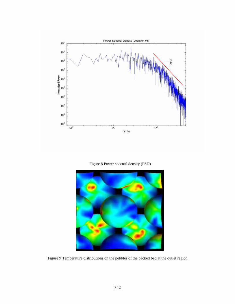
Figure 8 Power spectral density (PSD)

Figure 9 Temperature distributions on the pebbles of the packed bed at the outlet region

342

close similarity to those of water. More details can be obtained from reference 13. Schematic of the test facility is presented in Fig. 10.

The use of p-cymene allowed PTV measurements to be preformed at the center of the packed bed

square channel. The results in this investigation showed the velocity distribution at the pore scale level. Various pore geometries were observed at the column’s midplane. These geometries elucidate the complexity of the flow paths within the pore (Figure 11). Vortices were identified in the pores between beads. The preliminary results indicate that the amount and size of the vortices increased with the pore size and flow velocity. Vorticity maps were calculated from the obtained velocity fields at the pore level. Higher vorticity zones were identified near the boundary of the packing material.

Conclusion

Simulation of flow through the pebbles in the PBMR core was performed with large eddy

simulation techniques. The calculations manifested the complex flow structure within the gaps between the fuel pebbles. Vorticity in the y direction perpendicular to the flow was investigated. It was observed that eddies were created and destroyed fast between the pebbles. This was expected because of the high Reynolds number in this simulation. Although small time step was employed in LES simulations, suitability of transient time steps should investigated. The dynamic subgrid model should be studied to reveal the impact of SGS viscosity model on the flow predictions.

A preliminary experimental setup resembling the pebble bed core was constructed. Velocity field

between the pebble gaps using particle image velocimetry technique with fluid had the same refractive index of the glass pebbles. References

1. Lohnert, G., 1990. Technical design features and essential safety-related properties of the HTR-module, Nucl. Eng. Des. 121.

2. Lohnert, G., Reutler, H., 1983. The modular HTR-a new design of high temperature pebble bed reactor. J. Br. Nucl. Energy Soc. 22 (June (3)).197.

3. Rousseau, P.G., Greyvenstein G.P., 2002. One-dimensional reactor model for the integrated simulation of the PBMR power plant, in: J.P. Meyer (ed.), Proceedings of 1st Int. Conf. on Heat Transfer Fluid Mechanics and Thermodynamics, Kruger Park, South Africa.

4. Van Staden, M. P., Janse Van Rensburg C., Viljoen, C. F., 2002. CFD simulation of helium gas cooled pebble bed reactor, in: J.P. Meyer (ed.), Proceedings of 1st Int. Conf. on Heat Transfer Fluid Mechanics and Thermodynamics, Kruger Park, South Africa.

5. Calis H.P.A., Nijenhuis J., Paikert B.C., Dautzenberg F.M., Van Den Bleek C.M., 2001. CFD modeling and experimental validation of pressure drop and flow profile in a novel structured catalytic reactor packing. Chemical Engineering Science 56:1713-1720.

6. Patel, V. C., Sotiropoulos F., 1997. Longitudinal curvature effects in turbulent boundary

layers. Progress in Aerospace Sciences, 33, 1-70.

7. AEA Technology Engineering Software Ltd. (1996-2003) CFX5.6b User Manual http://www.cfx.aeat.com.

343

Figure 10 Experimental set-up

8. Pebble bed modular reactor (Pty) Ltd. PBMR Technical information. http://www.pbmr.com/

9. Yesilyurt, G., 2003. Numerical simulation of flow distribution for pebble bed high temperature gas cooled reactors. M.S. thesis, Texas A&M University.

10. Barsamian H. R., 2000. New near-wall models with dynamic subgrid scale closure for Large Eddy Simulation in curvilinear coordinates for complex geometries. Ph.D. dissertation, Texas A&M University, College Station, Texas.

Flow meter

Valve

High Power Laser

Pump

High resolution cameras

Packed Bed

Laser sheet

344

Figure 11 Example of the measured average velocity field inside the packed bed

11. Hassan, Y. A., Barsamian, H. R 2001. Near-wall modeling for complex flows using the large

eddy simulation techniques in curvilinear coordinates. International Journal of Heat and Mass Transfer, Vol. 44, issues 21, pp. 4009-4026.

12. Hassan, Y., A., and Barsamian, H. R., 2004. “Tube bundle flows with the large eddy simulation technique in curvilinear coordinates. International Journal of Heat and Mass Transfer, Vol. 47, issues 14-16, pp. 3057-3071, 2004.

13. Dominguez-Ontiveros, et al., 2005. PIV measurements in a matched refractive index packed bed. ANS Transaction, Vol. 93.

345

346