Laplace and Z transforms - Springer

3Laplace and Z transforms

3.1 The Laplace transform

Let f be a function defined on the interval R+ = [0,∞[. Alternatively, wecan think of f(t) as being defined for all real t, but satisfying f(t) = 0 forall t < 0. This can be expressed by writing

f(t) = f(t)H(t),

where H is the Heaviside function. Now let s be a real (or complex, if youlike) number. If the integral

f(s) =∫ ∞

0f(t) e−st dt (3.1)

exists (with a finite value), we say that it is the Laplace transform of f ,evaluated at the point s. We shall write, interchangeably, f(s) or L[f ](s).In applications, one also often uses the notation F (s) (capital letter for thetransform of the corresponding lower-case letter).

Example 3.1. Let f(t) = eat, t ≥ 0. Then,∫ ∞

0f(t) e−st dt =

∫ ∞

0eat−st dt =

[e(a−s)t

a− s

]∞

t=0=

1s− a

,

provided that a− s < 0 so that the evaluation at infinity yields zero. Thuswe have f(s) = 1/(s− a) for s > a, or

L[eat](s) =1

s− a, s > a.

40 3. Laplace and Z transforms

In particular, if a = 0, we have the Laplace transform of the constantfunction 1: it is equal to 1/s for s > 0. ��Example 3.2. Let f(t) = t, t > 0. Then, integrating by parts, we get

f(s) =∫ ∞

0t e−st dt =

[t · e

−st

−s]∞

t=0+

1s

∫ ∞

01 · e−st dt

= 0 +1sL[1](s) =

1s2.

This works for s > 0. ��It may happen that the Laplace transform does not exist for any real

value of s. Examples of this are given by f(t) = 1/t, f(t) = et2 .A profound understanding of the workings of the Laplace transform re-

quires considering it to be a so-called analytic function of a complex vari-able, but in most of this book we shall assume that the variable s is real. Weshall, however, permit the function f to take complex values: it is practicalto be allowed to work with functions such as f(t) = eiαt.

Furthermore, we shall assume that the integral (3.1) is not merely conver-gent, but that it actually converges absolutely. This enables us to estimateintegrals, using the inequality | ∫ f | ≤ ∫ |f |.Example 3.3. Let f(t) = eibt. Then we can imitate Example 3.1 aboveand write ∫ ∞

0f(t) e−st dt=

∫ ∞

0e(ib−s)t dt =

[e(ib−s)t

ib− s

]∞

t=0

=1

ib− s

[e−st(cos bt+ i sin bt)

]∞t=0.

For s > 0 the substitution as t → ∞ will tend to zero, because the factore−st tends to zero and the rest of the expression is bounded. The result isthus that L[eibt](s) = 1/(s − ib), which means that the formula that weproved in Example 3.1 holds true also when a is purely imaginary. It isleft to the reader to check that the same formula holds if a is an arbitrarycomplex number and s > Re a. ��

It would be convenient to have some simple set of conditions on a functionf that ensure that the Laplace transform is absolutely convergent for somevalue of s. Such a set of conditions is given in the following definition.

Definition 3.1 Let k be a positive number. Assume that f has the follow-ing properties:(i) f is continuous on [0,∞[ except possibly for a finite number of jump

discontinuities in every finite subinterval;(ii) there is a positive number M such that |f(t)| ≤ Mekt for all t ≥ 0.Then we say that f belongs to the class Ek. If f ∈ Ek for some value of k,we say that f ∈ E.

3.1 The Laplace transform 41

Using set notation we can say that E =⋃k>0

Ek. Condition (ii) means that

f grows at most exponentially; this word lies behind the use of the letterE. If f ∈ Ek for one value of k, then also f ∈ Ek for all larger k.

Theorem 3.1 If f ∈ Ek, then f(s) exists for all s > k.

Proof. We begin by observing that condition (i) for the class Ek impliesthat the integral ∫ T

0f(t) e−st dt

exists finitely for all s and all T > 0. Now assume s > k. Thus there existsa number M and a number t0 so that f(t)e−kt ≤ M for t > t0. Then wecan estimate as follows:∫ T

t0

|f(t)| e−st dt=∫ T

t0

|f(t)| e−kt e−(s−k)t dt ≤∫ T

t0

Me−(s−k)t dt

≤M

∫ ∞

t0

e−(s−k)t dt ≤ M

∫ ∞

0e−(s−k)t dt =

M

s− k< ∞.

This means that the generalized integral over [t0,∞[ converges absolutely,and then this is equally true for the integral over [0,∞[. ��

The result of the theorem can be “bootstrapped” in the following way.If σ0 = inf{k : f ∈ Ek}, then the Laplace transform exists for all s > σ0.Indeed, let k = (s + σ0)/2, so that σ0 < k < s; then f ∈ Ek (why?), andthe theorem can be applied. The number σ0 is a reasonably exact measureof the rate of growth of the function f . In what follows we shall sometimesuse the notation σ0 or σ0(f) for this measure.

As a consequence of the theorem we now know that a large set of commonfunctions do have Laplace transforms. Among them are, e.g., polynomials,trigonometric functions such as sin and cos and ordinary exponential func-tions; also sums and products of such functions. If you have studied simpledifferential equations you may recall that these functions are precisely thepossible solutions of homogeneous linear differential equations with con-stant coefficients, such as, for example,

y(v) + 4y(iv) − 8y′′′ + 15y′′ − 24y′ = 0.

We shall soon see that Laplace transforms give us a new technique for solv-ing these equations. We shall also be able to solve more general problems,like integral equations of this kind:∫ t

0f(t− x) f(x) dx+ 3

∫ t

0f(x) dx+ 2t = 0, t > 0. (3.2)

Another consequence of the theorem is worth emphasizing: if a Laplacetransform exists for one value of s, then it is also defined for all larger


values of s. If we are dealing with several different transforms having variousdomains, we can always be sure that they are all defined at least in onecommon semi-infinite interval. It is customary to be rather sloppy aboutspecifying the domains of definition for Laplace transforms: we make a tacitagreement that s is large enough so that all transforms occuring in a givensituation are defined.

Exercises3.1 Let f(t) = et2 , g(t) = e−t2 . Show that f /∈ E, whereas g ∈ Ek for all k.3.2 Compute the Laplace transform of f(t) = eat, where a = α + iβ is a

complex constant.3.3 Let f(t) = sin t for 0 ≤ t ≤ π, f(t) = 0 otherwise. Find f(s).

3.2 Operations

The Laplace transformation obeys some simple rules of computation andalso some less simple rules. The simplest ones are collected in the follow-ing table. Everywhere we assume that s takes sufficiently large values, asdiscussed at the end of the preceding section.

1. L[αf + βg](s) = αf(s) + βg(s), if α and β are constants.

2. L[eatf(t)](s) = f(s− a), if a is a constant (damping rule).

3. If we define f(t) = 0 for t < 0 and if a > 0, then

L[f(t− a)](s) = e−asf(s) (delaying rule).

4. L[f(at)](s) =1af(s/a), if a > 0.

The proofs of these rules are easy. As an example we give the computa-tions that yield rules 3 and 4:

L[f(t− a)](s) =∫ ∞

0f(t− a) e−st dt

u= t− adu= dt

t = 0 ⇔ u = −a

=∫ ∞

−a

f(u) e−s(u+a) du = e−as

∫ ∞

−a

f(u) e−su du

= e−as

∫ ∞

0f(u) e−su du = e−asf(s);

L[f(at)](s) =∫ ∞

0f(at) e−st dt

{u= atdu= a dt

}=∫ ∞

0f(u) e−s·u/a du

a

=1a

∫ ∞

0f(u) exp

(− s

a· u)du =

1af

(s

a

).

3.2 Operations 43

Example 3.4. Using rule 1 and the result of Example 3.3 in the precedingsection, we can find the Laplace transforms of cos and sin:

L[cos bt](s) = 12L[eibt + e−ibt](s) = 1

2

(1

s− ib+

1s+ ib

)=

s

s2 + b2,

L[sin bt](s) =12i

L[eibt − e−ibt](s) =12i

(1

s− ib− 1s+ ib

)=

b

s2 + b2.

��Example 3.5. Applying rule 2 to the result of Example 3.4 we get

L[eat cos bt](s) =s− a

(s− a)2 + b2, L[eat sin bt](s) =

b

(s− a)2 + b2.

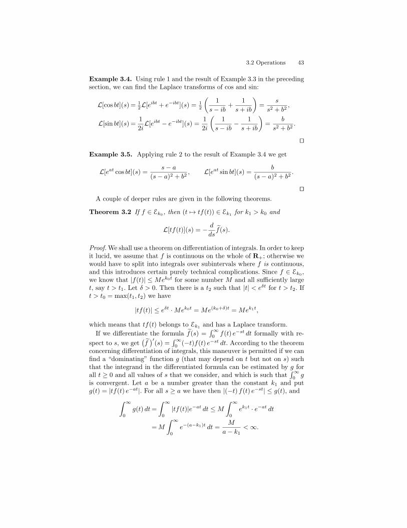
��A couple of deeper rules are given in the following theorems.

Theorem 3.2 If f ∈ Ek0 , then (t �→ tf(t)) ∈ Ek1 for k1 > k0 and

L[tf(t)](s) = − d

dsf(s).

Proof. We shall use a theorem on differentiation of integrals. In order to keepit lucid, we assume that f is continuous on the whole of R+; otherwise wewould have to split into integrals over subintervals where f is continuous,and this introduces certain purely technical complications. Since f ∈ Ek0 ,we know that |f(t)| ≤ Mek0t for some number M and all sufficiently larget, say t > t1. Let δ > 0. Then there is a t2 such that |t| < eδt for t > t2. Ift > t0 = max(t1, t2) we have

|tf(t)| ≤ eδt ·Mek0t = Me(k0+δ)t = Mek1t,

which means that tf(t) belongs to Ek1 and has a Laplace transform.If we differentiate the formula f(s) =

∫∞0 f(t) e−st dt formally with re-

spect to s, we get(f)′(s) =

∫∞0 (−t)f(t) e−st dt. According to the theorem

concerning differentiation of integrals, this maneuver is permitted if we canfind a “dominating” function g (that may depend on t but not on s) suchthat the integrand in the differentiated formula can be estimated by g forall t ≥ 0 and all values of s that we consider, and which is such that

∫∞0 g

is convergent. Let a be a number greater than the constant k1 and putg(t) = |tf(t) e−at|. For all s ≥ a we have then |(−t) f(t) e−st| ≤ g(t), and∫ ∞

0g(t) dt=

∫ ∞

0|tf(t)|e−at dt ≤ M

∫ ∞

0ek1t · e−at dt

=M

∫ ∞

0e−(a−k1)t dt =

M

a− k1< ∞.


This shows that the conditions for differentiating formally are fulfilled, andthe theorem is proved. ��Example 3.6. We know that L[1](s) = 1/s for s > 0. Then we can saythat

L[t](s) = L[t · 1](s) = − d

ds

1s

= −(

− 1s2

)=

1s2, s > 0.

Repeating this argument (do it!) we find that

L[tn](s) =n!sn+1 , s > 0.

��Example 3.7. Also, rule 2 allows us to conclude that

L[tn eat](s) =n!

(s− a)n+1 , s > 0.

��A sort of reverse of Theorem 3.2 is the following. The notation f(0+)

stands for the right-hand limit limt→0+

f(t) = limt↘0

f(t).

Theorem 3.3 Assume that f ∈ E is continuous on R+. Also assume thatthe derivative f ′(t) exists for all t ≥ 0 (with f ′(0) interpreted as the right-hand derivative) and that f ′ ∈ E. Then

L[f ′](s) = s f(s) − f(0+).

Proof. Suppose that f ∈ Ek0 and f ′ ∈ Ek1 , and take s to be larger thanboth k0 and k1. Let T be a positive number. Integration by parts gives∫ T

0f ′(t) e−st dt = f(T ) e−sT − f(0+) e0 + s

∫ T

0f(t) e−st dt.

When T → ∞, the first term in the right-hand member tends to zero, andthe result is the desired formula. ��

Theorem 3.3 will be used for solving differential equations.

The following theorem states a few additional properties of the Laplacetransform.

Theorem 3.4 (a) If f ∈ E, then

lims→∞ f(s) = 0. (3.3)

(b) The initial value rule: If f(0+) exists, then

lims→∞ sf(s) = f(0+). (3.4)

3.2 Operations 45

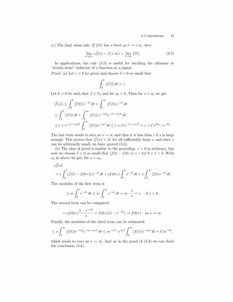
(c) The final value rule: If f(t) has a limit as t → +∞, then

lims↘0+

sf(s) = f(+∞) = limt→∞ f(t). (3.5)

In applications, the rule (3.5) is useful for deciding the ultimate or“steady-state” behavior of a function or a signal.Proof. (a) Let ε > 0 be given and choose δ > 0 so small that∫ δ

0|f(t)| dt < ε.

Let k > 0 be such that f ∈ Ek and let s0 > k. Then for s > s0 we get

|f(s)| ≤∫ δ

0|f(t)| e−st dt+

∫ ∞

δ

|f(t)| e−st dt

≤∫ δ

0|f(t)| dt+

∫ ∞

δ

|f(t)| e−s0te−(s−s0)t dt

≤ ε+ e−(s−s0)δ∫ ∞

δ

|f(t)|e−s0t dt ≤ ε+ Ce−(s−s0)δ = ε+ Ceδs0 · e−δs.

The last term tends to zero as s → ∞ and thus it is less than ε if s is largeenough. This proves that |f(s)| < 2ε for all sufficiently large s, and since εcan be arbitrarily small, we have proved (3.3).

(b) The idea of proof is similar to the preceding. ε > 0 is arbitrary, butnow we choose δ > 0 so small that |f(t) − f(0+)| < ε for 0 < t < δ. Withs0 as above we get, for s > s0,

sf(s)

= s

∫ δ

0(f(t) − f(0+)) e−st dt+ sf(0+)

∫ δ

0e−st dt+ s

∫ ∞

δ

f(t) e−st dt.

The modulus of the first term is

≤ sε

∫ δ

0e−st dt ≤ sε

∫ ∞

0e−st dt = sε · 1

s= ε, if s > 0.

The second term can be computed:

= sf(0+)1 − e−sδ

s= f(0+)(1 − e−sδ) → f(0+) as s → ∞.

Finally, the modulus of the third term can be estimated:

≤ s

∫ ∞

δ

|f(t)|e−s0te−(s−s0)t dt ≤ se−sδ · es0δ

∫ ∞

δ

|f(t)| e−s0t dt = Cse−δs,

which tends to zero as s → ∞. Just as in the proof of (3.3) we can drawthe conclusion (3.4).


(c) This proof also runs along similar paths. We begin by writing

sf(s) = s

∫ T

0f(t) e−st dt+ s

∫ ∞

T

(f(t) − f(∞))e−st dt+ f(∞)e−sT .

Choose T so large that |f(t) − f(∞)| < ε for t ≥ T . The modulus of the

first term can be estimated by s∫ T

0 |f | → 0 as s → 0+, and the modulusof the second one is

≤ s

∫ ∞

T

ε · e−st dt = ε e−sT ≤ ε.

The proof is finished in an analogous way to the others. ��We round off this section by a generalization of the rule for Laplace

transformation of a power t (cf. Example 3.6). To this end we need a gener-alization of factorials to non-integers. This is provided by Euler’s Gammafunction, whis is defined by

Γ(x) =∫ ∞

0ux−1e−u du, x > 0.

It is easy to see that this integral converges for positive x. It is also easyto see that Γ(1) = 1. Integrating by parts we find

Γ(x+ 1) =∫ ∞

0uxe−u du =

[−uxe−u

]∞

0+ x

∫ ∞

0ux−1e−u du = xΓ(x).

From this we deduce that Γ(2) = 1 · Γ(1) = 1, Γ(3) = 2, and, by induction,Γ(n + 1) = n! for integral n. Thus, this function can be viewed as aninterpolation of the factorial.

Now we let f(t) = ta, where a > −1. It is then clear that f has a Laplacetransform, and we find, for s > 0,

f(s) =∫ ∞

0tae−st dt

{st = udt = du/s

}=∫ ∞

0

(us

)ae−u du

s

=1

sa+1

∫ ∞

0uae−u du =

Γ(a+ 1)sa+1 .

If a is an integer, this reduces to the formula of Example 3.6.

Exercises3.4 Find the Laplace transforms of (a) 2t2 − e−t

(b) (t2 + 1)2 (c) (sin t− cos t)2 (d) cosh2 4t (e) e2t sin 3t (f) t3 sin 3t.

3.5 Compute the Laplace transform of f(t) =

{1/ε for 0 < t < ε,

0 otherwise.

3.6 Find the transform of f(t) =

{(t− 1)2 for t > 1,0 otherwise.

3.3 Applications to differential equations 47

3.7 Solve the same problem for f(t) =∫ t

0

1 − e−u

udu.

3.8 Compute∫ ∞

0

t e−3t sin t dt. (Hint: f(3) !)

3.9 Find the Laplace transform of f , if we define f(t) = t sin t for 0 ≤ t ≤ π,f(t) = 0 otherwise. (Hint: use the result of Exercise 3.3, p. 42.)

3.10 Find the Laplace transform of the function f defined by

f(t) = na for n− 1 ≤ x < n, n = 1, 2, 3, . . . .

3.11 Compute L[te−t sin t](s).

3.12 Explain why the functions2

s2 + 1cannot be the Laplace transform of any

f ∈ E.

3.13 Show that if f is periodic with period a, then

f(s) =1

1 − e−as

∫ a

0

f(t) e−st dt.

(Hint:∫∞0

=∑∞

0

∫ a(k+1)

ak. Let u = t− ak, use the formula for the sum of

a geometric series.)

3.14 Find the Laplace transform of the function with period 1 that is describedby f(t) = t for 0 < t < 1.

3.15 Verify the final value rule (3.5) for f(s) = 1/(s(s+ 1)) by comparing f(t)and lim

s→0+sf(s).

3.16 Prove that Γ(

12

)=

√π. What are the values of Γ

(32

)and Γ

(52

)?

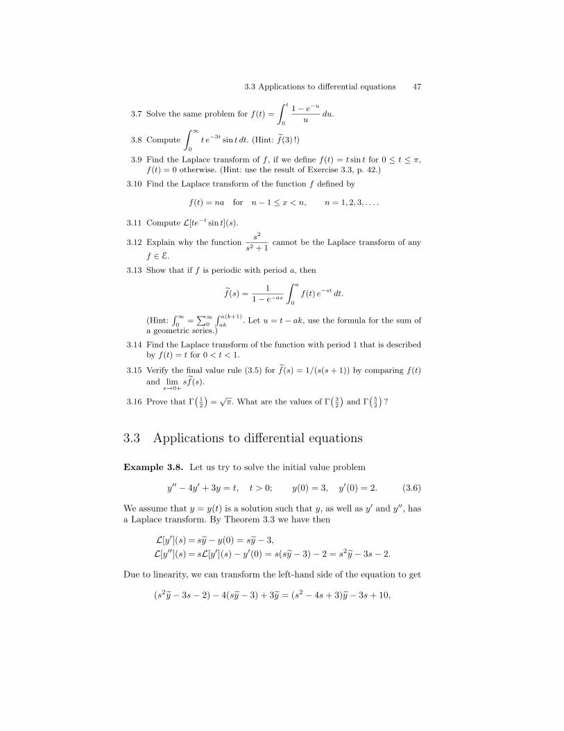
3.3 Applications to differential equations

Example 3.8. Let us try to solve the initial value problem

y′′ − 4y′ + 3y = t, t > 0; y(0) = 3, y′(0) = 2. (3.6)

We assume that y = y(t) is a solution such that y, as well as y′ and y′′, hasa Laplace transform. By Theorem 3.3 we have then

L[y′](s) = sy − y(0) = sy − 3,L[y′′](s) = sL[y′](s) − y′(0) = s(sy − 3) − 2 = s2y − 3s− 2.

Due to linearity, we can transform the left-hand side of the equation to get

(s2y − 3s− 2) − 4(sy − 3) + 3y = (s2 − 4s+ 3)y − 3s+ 10,


and this must be equal to the transform of the right-hand side, which is1/s2. The result is an algebraic equation, which we can solve for y:

(s2 −4s+3)y−3s+10 =1s2

⇐⇒ y =3s3 − 10s2 + 1s2(s2 − 4s+ 3)

=3s3 − 10s2 + 1s2(s− 1)(s− 3)

.

The last expression can be expanded into partial fractions. Assume that

3s3 − 10s2 + 1s2(s− 1)(s− 3)

=A

s2+B

s+

C

s− 1+

D

s− 3.

Multiplying by the common denominator and identifying coefficients wefind that A = 1

3 , B = 49 , C = 3, and D = − 4

9 . Thus we have

y = 13 · 1

s2+ 4

9 · 1s

+ 3 · 1s− 1

− 49 · 1

s− 3.

It so happens that there exists a function with precisely this Laplace trans-form, namely, the function

z = 13 t+ 4

9 + 3et − 49e

3t.

Could it be the case that y = z ? One way of finding this out is by differ-entiating and investigating if indeed z does satisfy the equation and initialconditions. And it does (check for yourself)! By the general theory of dif-ferential equations, the problem (3.6) has a unique solution, and it followsthat z must be the solution we are looking for. ��

The example demonstrates a very useful method for treating linear in-titial value problems. There is one difficulty that is revealed at the end ofthe example: could it be possible that two different functions might havethe same Laplace transform? This question is answered by the followingtheorem.

Theorem 3.5 (Uniqueness for Laplace transforms) If f and g bothbelong to E, and f(s) = g(s) for all (sufficiently) large values of s, thenf(t) = g(t) for all values of t where f and g are continuous.

We omit the proof of this at this point. It is given in Sec. 7.10. In thatsection we also prove a formula for the reconstruction of f(t) when f(s)is known — a so-called inversion formula for the Laplace transform. Thepresent theorem, however, gives us the possibility to invert Laplace trans-forms by recognizing functions, just as we did in the example.

This requires that we have access to a table of Laplace transforms ofsuch functions that can be expected to occur. Such a table is found at theend of the book (p. 247 ff), and similar tables are included in all decenthandbooks on the subject. Several of the entries in such tables have alreadybeen proved in the examples of this chapter; others can be done as exercisesby the interested student.


We point out that the uniqueness result as such does not rule out thepossibility that a differential equation (or other problem) may have solu-tions that have no Laplace transforms, e.g., solutions that grow faster thanexponentially. To preclude such solutions one must look into the theoryof differential equations. For linear equations there is a result on uniquesolutions for initial value problems, which may serve the purpose. If thecoefficients are constants and the equation is homogeneous, one actuallyknows that all solutions have at most exponential growth.

The Laplace transform method is ideally adapted to solving initial valueproblems. Strictly speaking, the method takes into consideration only whatgoes on for t ≥ 0. Very often, however, the expressions obtained for thesolutions are also valid for t < 0.

We include some examples on using a table of Laplace transforms in afew more complicated situations. The technique may remind the reader ofthe integration of rational functions.

Example 3.9. Find f(t), when f(s) =2s+ 3

s2 + 4s+ 13.

Solution. Complete the square in the denominator: s2+4s+13 = (s+2)2+9.Then split the numerator to enable us to recognize transforms of cosinesand sines:

2s+ 3s2 + 4s+ 13

=2(s+ 2) − 1(s+ 2)2 + 32 = 2 · s+ 2

(s+ 2)2 + 32 − 13 · 3

(s+ 2)2 + 32 ,

and now we can see that this is the transform of f(t) = 2e−2t cos 3t −13e

−2t sin 3t. ��

Example 3.10. Find g(t), if g(s) =2s

(s2 + 1)2.

Solution. We recognize the transform as a derivative:

g(s) = − d

ds

1s2 + 1

.

By Theorem 3.2 and the known transform of the sine we get g(t) = t sin t.��

Example 3.11. Solve the initial value problem

y′′ + 4y′ + 13y = 13, y(0) = y′(0) = 0.

Solution. Transformation gives

(s2 + 4s+ 13)y =13s

⇐⇒ y =13

s((s+ 2)2 + 9

) .


Expand into partial fractions:

y =1s

− s+ 4(s+ 2)2 + 9

=1s

− s+ 2(s+ 2)2 + 9

− 23 · 3

(s+ 2)2 + 9.

The solution is found to be

y(t) =(1 − e−2t(cos 3t+ 2

3 sin 3t))H(t).

(Here we have multiplied the result by a Heaviside factor, to indicate thatwe are considering the solution only for t ≥ 0. This factor is often omitted.Whether or not it should be there is often a matter of dispute among usersof the transform.) ��

We can also treat systems of differential equations.

Example 3.12. Solve the initial value problem{x′ = x+ 3y,y′ = 3x+ y;

x(0) = 5, y(0) = 1.

Solution. Laplace transformation gives{sx− 5 = x+ 3ysy − 1 = 3x+ y

⇐⇒{

(1 − s)x+ 3y = −53x+ (1 − s)y = −1

We can, for example, solve the second equation for x = 13 (s− 1)y − 1

3 andsubstitute this into the first, whereupon simplification yields (s2−2s−8)y =s+ 14 and

y =s+ 14

(s− 4)(s+ 2)=

3s− 4

− 2s+ 2

.

We see that y = 3e4t − 2e−2t, and then we deduce, in one way or another,that x = 3e4t +2e−2t. (Think of at least three different ways of performingthis last step!) ��

Finally, we demonstrate how even a partial differential equation can betreated by Laplace transforms. The trick is to transform with respect to oneof the independent variables and let the others stand. Using this techniqueoften involves taking rather bold chances in the hope that rules of compu-tation be valid. One way of regarding this is to view it precisely as takingchances – if we arrive at a tentative solution, it can always be checked bysubstitution in the original problem.

Example 3.13. Find a solution of the problem

∂2u

∂x2 =∂u

∂t, 0 < x < 1, t > 0;

u(0, t) = 1, u(1, t) = 1, t > 0;u(x, 0) = 1 + sinπx, 0 < x < 1.


Solution. We introduce the Laplace transform U(x, s) of u(x, t), i.e.,

U(x, s) = L[t �→ u(x, t)](s) =∫ ∞

0u(x, t) e−st dt.

Here, x is thought of as a constant. Then we change our attitude andassume that this integral can be differentiated with respect to x, indeedtwice, so that

∂2U

∂x2 =∂2

∂x2

∫ ∞

0u(x, t) e−st dt =

∫ ∞

0

∂2

∂x2u(x, t) e−st dt.

The differential equation is then transformed into

∂2U

∂x2 = sU − (1 + sinπx), 0 < x < 1,

and the boundary conditions into

U(0, s) =1s, U(1, s) =

1s.

Now we switch attitudes again: think of s as a constant and solve theboundary value problem. Just to feel comfortable we could write the equa-tion as

U ′′ − sU = −1 − sinπx. (3.7)

The homogeneous equation has a characteristic equation r2 − s = 0 andits solution is UH = Aex

√s + Be−x

√s. (Here, the “constants” A and B

are in general functions of s.) A particular solution to the inhomogeneousequation could have the form UP = a + b sinπx + c cosπx, and insertionand identification gives a = 1/s, b = 1/(s + π2), c = 0. Thus the generalsolution of (3.7) is

U(x, s) = A(s)ex√

s +B(s)e−x√

s +1s

+sinπxs+ π2 .

The boundary conditions force us to take A(s) = B(s) = 0, so we are left

with U(x, s) =1s

+sinπxs+ π2 . Now we again consider x as a constant and

recognize that U is the Laplace transform of u(x, t) = 1 + e−π2t sinπx.The fact that this function really does solve the original problem must bechecked directly (since we have made an assumption on differentiability ofan integral, which might have been too bold). ��Remark. This problem can also be attacked by other methods developed in laterparts of the book (Chapter 6). ��


Exercises

3.17 Invert the following Laplace transforms: (a)1

s(s+ 1)(b)

3(s− 1)2

(c)1

s(s+ 2)2(d)

5s2(s− 5)2

(e)1

(s− a)(s− b)(f)

1s2 + 4s+ 29

.

3.18 Use partial fractions to find f when f(s) is given by(a) s−2(s+ 1)−1, (b) b2s−1(s2 + b2)−1, (c) s(s− 3)−5,(d) (s2 + 2)s−1(s+ 1)−1(s+ 2)−1.

3.19 Invert the following Laplace transforms: (a)1 + e−s

s(b)

e−s

(s− 1)(s− 2)

(c) lns+ 3s+ 2

(d) lns2 + 1s(s+ 3)

(e)s+ 1s4/3 (f)

√s− 1s

.

3.20 Solve the initial value problem y′′ + y = 2et, t > 0, y(0) = y′(0) = 2.

3.21 Solve the initial value problem

{y′′(t) − 2y′(t) + y(t) = t et sin t,y(0) = 0, y′(0) = 0.

3.22 Solve

{y(3)(t) − y′′(t) + 4y′(t) − 4y(t) = −3et + 4e2t,

y(0) = 0, y′(0) = 5, y′′(0) = 3.

3.23 Solve the system

x′(t) + y′(t) = t,

x′′(t) − y(t) = e−t,

x(0) = 3, x′(0) = −2, y(0) = 0.

3.24 Solve the system

x′(t) − y′(t) − 2x(t) + 2y(t) = sin t,x′′(t) + 2y′(t) + x(t) = 0,x(0) = x′(0) = y(0) = 0.

3.25 Solve the problem

y′′(t) − 3y′(t) + 2y(t) =

{1, t > 20, t < 2

; y(0) = 1, y′(0) = 0.

3.26 Solve the systemdy

dt= 2z − 2y + e−t

dz

dt= y − 3z

t > 0; y(0) = 1, z(0) = 2.

3.27 Solve the differential equation

2y(iv) + y′′′ − y′′ − y′ − y = t+ 2, t > 0,

with initial conditions y(0) = y′(0) = 0, y′′(0) = y′′′(0) = 1.

3.28 Solve the differential equation

y′′ + 3y′ + 2y = e−t sin t, t > 0; y(0) = 1, y′(0) = −3.

3.4 Convolution 53

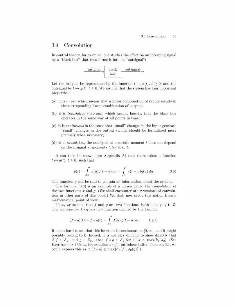
3.4 Convolution

In control theory, for example, one studies the effect on an incoming signalby a “black box” that transforms it into an “outsignal”:

insignal black outsignal→ →box

Let the insignal be represented by the function t �→ x(t), t ≥ 0, and theoutsignal by t �→ y(t), t ≥ 0. We assume that the system has four importantproperties:

(a) it is linear, which means that a linear combination of inputs results inthe corresponding linear combination of outputs;

(b) it is translation invariant, which means, loosely, that the black boxoperates in the same way at all points in time;

(c) it is continuous in the sense that “small” changes in the input generate“small” changes in the output (which should be formulated moreprecisely when necessary);

(d) it is causal, i.e., the outsignal at a certain moment t does not dependon the insignal at moments later than t.

It can then be shown (see Appendix A) that there exists a functiont �→ g(t), t ≥ 0, such that

y(t) =∫ t

0x(u)g(t− u) du =

∫ t

0x(t− u)g(u) du. (3.8)

The function g can be said to contain all information about the system.The formula (3.8) is an example of a notion called the convolution of

the two functions x and g. (We shall encounter other versions of convolu-tion in other parts of this book.) We shall now study this notion from amathematical point of view.

Thus, we assume that f and g are two functions, both belonging to E.The convolution f ∗ g is a new function defined by the formula

(f ∗ g)(t) = f ∗ g(t) =∫ t

0f(u) g(t− u) du, t ≥ 0.

It is not hard to see that this function is continuous on [0,∞[, and it mightpossibly belong to E. Indeed, it is not very difficult to show directly thatif f ∈ Ek1 and g ∈ Ek2 , then f ∗ g ∈ Ek for all k > max(k1, k2). (SeeExercise 3.38.) Using the notation σ0(f), introduced after Theorem 3.1, wecould express this as σ0(f ∗ g) ≤ max

(σ0(f), σ0(g)

).)


Convolution can be regarded as an operation for functions, a sort of“multiplication.” For this operation a few simple rules hold; the reader isinvited to check them out:

f ∗ g = g ∗ f (commutative law)f ∗ (g ∗ h) = (f ∗ g) ∗ h (associative law)f ∗ (g + h) = f ∗ g + f ∗ h (distributive law)

Example 3.14. Let f(t) = et, g(t) = e−2t. Then

f ∗ g(t) =∫ t

0eu e−2(t−u) du =

∫ t

0eu−2t+2u du = e−2t

∫ t

0e3u du

= e−2t[ 13 e

3u]u=t

u=0 = 13e

−2t(e3t − 1

)=et − e−2t

3.

��Example 3.15. If g(t) = 1, then f ∗g(t) =

∫ t

0 f(u) du. Thus, “integration”can be considered to be convolution with the function 1. ��

When dealing with convolutions, the Laplace transform is useful becauseof the following theorem.

Theorem 3.6 The Laplace transform of a convolution is the product ofthe Laplace transforms of the two convolution factors:

L[f ∗ g](s) = f(s) g(s).

Proof. Let s be so large that both f(s) and g(s) exist. We have agreedin section 3.1 that this means that the corresponding integrals convergeabsolutely. Now consider the improper double integral∫∫

Q

|f(u)g(v)|e−s(u+v) du dv,

where Q is the first quadrant in the uv plane. The integrated function beingpositive, the integral can be calculated just as we choose. For example, wecan write∫∫

Q

|f(u)g(v)|e−s(u+v) du dv =∫ ∞

0du

∫ ∞

0|f(u)||g(v)|e−sue−sv dv

=∫ ∞

0|f(u)|e−su du

∫ ∞

0|g(v)|e−sv dv.

The two one-dimensional integrals here are assumed to be convergent,which means that the double integral also converges. But this in turn meansthat the improper double integral without modulus signs,

Φ(s) =∫∫

Q

f(u)g(v)e−s(u+v) du dv

3.4 Convolution 55

is absolutely convergent. It can then also be computed in any manner, andwe do it in two ways. One way is imitating the previous calculation:

Φ(s) =∫ ∞

0du

∫ ∞

0f(u)g(v)e−sue−sv dv

=∫ ∞

0f(u)e−su du

∫ ∞

0g(v)e−sv dv = f(s) g(s).

Another way is integrating on triangles DT : u ≥ 0, v ≥ 0, u+ v ≤ T . But∫ T

0f ∗ g(t)e−st dt =

∫ T

0

(∫ t

0f(u)g(t− u) du

)e−su dt

=∫ T

0dt

∫ t

0f(u)e−su g(t− u)e−s(t−u) du

=∫ T

0f(u)e−su du

∫ T

u

g(t− u)e−s(t−u) dt ={t− u = vdt = dv

}=∫ T

0f(u)e−su du

∫ T−u

0g(v)e−sv dv

=∫∫DT

f(u)g(v)e−sue−sv du dv → Φ(s)

as T → ∞. This proves the formula in the theorem. ��Example 3.16. As an illustration of the theorem we can take the situationin Example 3.14. There we have

f(s) =1

s− 1, g(s) =

1s+ 2

,

f(s)g(s) =1

(s− 1)(s+ 2)=

13

s− 1−

13

s+ 2= L[f ∗ g](s).

��Example 3.17. Find a function f that satisfies the integral equation

f(t) = 1 +∫ ∞

0f(t− u) sinu du, t ≥ 0.

Solution. Suppose that f ∈ E. Then we can transform the equation to get

f(s) =1s

+ f(s) · 1s2 + 1

,

from which we solve

f(s) =s2 + 1s2

· 1s

=s2 + 1s3

=1s

+1s3,


and we see that f(t) = 1 + 12 t

2 ought to be a solution. Indeed it is, be-cause this function belongs to E, and then our successive steps make up asequence of equivalent statements. (It is also possible to check the solutionby substitution in the given integral equation. This should be done, if timepermits.) ��

Exercises

3.29 Calculate directly the convolution of eat and ebt (consider separately thecases a �= b and a = b). Check the result by taking Laplace transforms.

3.30 Use the convolution formula to determine f if f(s) is given by(a) s−1(s+ 1)−1, (b) s−1(s2 + a2)−1.

3.31 Find a function with the Laplace transforms2

(s2 + 1)2.

3.32 Find a function f such that∫ x

0

e−y cos y f(x− y) dy = x2 e−x, x ≥ 0.

3.33 Find a solution of the integral equation∫ t

0

(t− u)2f(u) du = t3, t ≥ 0.

3.34 Find two solutions of the integral equation (3.2) on page 41.

3.35 Find a function y(t) that satisfies y(0) = 0 and

2∫ t

0

(t− u)2 y(u) du+ y′(t) = (t− 1)2 for t > 0.

3.36 Find a function f(t) for t ≥ 0, that satisfies

f(0) = 1, f ′(t) + 3f(t) +∫ t

0

f(u)eu−t du =

{0, 0 ≤ t < 2,1, t > 2

.

3.37 Find a solution f of the integral-differential equation

5e−t

∫ t

0

ey cos 2(t− y) f(y) dy = f ′(t) + f(t) − e−t, f(0) = 0.

3.38 Prove the following result: if f ∈ Ek1 and g ∈ Ek2 , then f ∗ g ∈ Ek for allk > max{k1, k2}.

3.5 *Laplace transforms of distributions 57

3.5 *Laplace transforms of distributions

Laplace transforms can be used in the study of physical phenomena thattake place in a time interval that starts at a certain moment, at which theclock is set to t = 0. It is possible to allow the functions to include instan-taneous pulses and even more far-reaching generalizations of the classicalnotion of a function – i.e., to allow so-called distributions into the game.When we do so, it will normally be a good thing to allow such things tohappen also at the very moment t = 0, so we modify slightly the definitionof the Laplace transform into the following formula:

f(s) =∫ ∞

0−f(t)e−st dt = lim

ε↘0

∫ ∞

−ε

f(t)e−st dt.

If f is an ordinary function, the modified definition agrees with the formerone. But if f is a distribution, something new may occur.

As an example, let δa(t) be the Dirac pulse at the point a, where a ≥ 0.Then

δa(s) =∫ ∞

0−δa(t)e−st dt = e−as.

In particular, if a = 0, we get δ(s) = 1. We see that the rule that a Laplacetransform must tend to zero as s → ∞ no longer need hold for transformsof distributions.

The formula for the transform of a derivative must also be slightly mod-ified. Indeed, integration by parts gives

f ′(s) =∫ ∞

0−f ′(t)e−st dt =

[f(t)e−st

]∞

0−+s

∫ ∞

0−f(t)e−st dt = sf(s)−f(0−),

where f(0−) is the left-hand limit of f(t) at 0. This may cause some confu-sion when dealing with functions that are considered to be zero for negativet but nonzero for positive t. In this case it may now happen that f ′ includesa multiple of δ, which explains the different appearance of the formula. Inthis situation, it is preferable to be very explicit in supplying the factorH(t) in the description of functions.

Example 3.18. Solve the initial value problem

y′′ + 4y′ + 13y = δ′(t), y(0−) = y′(0−) = 0.

Solution. Transformation gives

(s2+4s+13)y = s ⇐⇒ y =s

(s+ 2)2 + 9=

s+ 2(s+ 2)2 + 9

− 23· 3(s+ 2)2 + 9

.


The solution is found to be

y(t) = e−2t(cos 3t− 23 sin 3t)H(t).

We check it by differentiating:

y′(t) = e−2t(−2 cos 3t+ 43 sin 3t− 3 sin 3t− 2 cos 3t)H(t) + δ(t)

= e−2t(−4 cos 3t− 53 sin 3t)H(t) + δ(t),

y′′(t) = e−2t(8 cos 3t+ 103 sin 3t+ 12 sin 3t− 5 cos 3t)H(t) − 4δ(t) + δ′(t)

= e−2t(3 cos 3t+ 463 sin 3t)H(t) − 4δ(t) + δ′(t).

Substituting this into the left-hand member of the equation, one sees thatit indeed solves the problem. ��Example 3.19. Find the general solution of the differential equationy′′ + 3y′ + 2y = δ.

Solution. It should be wellknown that the solution can be written as thesum of the general solution yH of the corresponding homogeneous equationy′′ +3y′ +2y = 0, and one particular solution yP of the given equation. Weeasily find yH = C1e

−t +C2e−2t, and proceed to look for yP . In doing this

we assume that yP (0−) = y′P (0−) = 0, which gives the simplest Laplace

transforms. Indeed, y′P = syP and y′′

P = s2yP , so that

s2yP + 3syP + 2yP = 1 ⇐⇒ yP =1

(s+ 1)(s+ 2)=

1s+ 1

− 1s+ 2

.

Thus it turns out that

yP =(e−t − e−2t

)H(t).

This means that the solution of the given problem is

y =C1e−t + C2e

−2t +(e−t − e−2t

)H(t)

= (C1+H(t))e−t + (C2−H(t))e−2t

={C1e

−t + C2e−2t, t < 0,

(C1 + 1)e−t + (C2 − 1)e−2t, t > 0.

We can see that in each of the intervals t < 0 and t > 0 these expressionsare solutions of the homogeneous equation, which is in accordance withthe fact that δ = 0 in the intervals. What happens at t = 0 is that theconstants change value in such a way that the first derivative has a jumpdiscontinuity and the second derivative contains a δ pulse (draw pictures!).

��The particular solution yP found in the preceding problem is called a

fundamental solution of the equation. Let us now denote it by E; thus,

E(t) =(e−t − e−2t

)H(t).

3.5 *Laplace transforms of distributions 59

It is useful in the following situation. Let f be any function, continuous fort ≥ 0. We want to find a solution of the problem y′′ + 3y′ + 2y = f . If weassume y(0−) = y′(0−) = 0, we get

y =f(s)

s2 + 3s+ 2= f(s) · 1

s2 + 3s+ 2= f(s)E(s).

This means that y can be found as the convolution of f and E:

y(t) = f ∗ E(t) =∫ t

0f(t− u)

(e−u − e−2u

)du.

The fundamental solution thus provides a means for finding a particularsolution for any inhomogeneuous equation with the given left-hand side.

This idea can be applied to any linear differential equation with constantcoefficients. The left-hand member of such an equation can be written inthe form P (D)y, where D is the differentiation operator and P (·) is apolynomial. For example, if P (r) = r2 + 3r + 2, then

P (D)y = (D2 + 3D + 2)y = y′′ + 3y′ + 2y.

The fundamental solution E is, in the general case, the function such that

E(s) =1

P (s), E(t) = 0 for t < 0.

Exercises

3.39 Find a solution of the differential equation y′′′ +3y′′ +3y′ +y = H(t−1)+δ(t− 2), that satisfies y(0) = y′(0) = y′′(0) = 0.

3.40 Solve the differential equation y′′ +4y′ +5y = δ(t), y(t) = 0 for t < 0. Thendeduce a formula for a particular solution of the equation y′′ + 4y′ + 5y =f(t), where f is any continuous function such that f(t) = 0 for t < 0.

3.41 Find fundamental solutions for the following equations: (a) y′′ + 4y = δ,(b) y′′ + 4y′ + 8y = δ, (c) y′′′ + 3y′′ + 3y′ + y = δ.

3.42 Find a function y such that y(t) = 0 for t ≤ 0 and

y′(t) + 3y(t) + 2∫ t

0

y(u) du = 2(H(t− 1) −H(t− 2)

)for t > 0.

3.43 Find a function f(t) such that f(t) = 0 for t < 0 and

e−t

∫ t+

0−f(p) ep dp− f(t) + f ′(t) = δ(t) − t e−t H(t), −∞ < t < ∞.


3.6 The Z transform

In this section we sketch the theory of a discrete analogue of the Laplacetransform. We have so far been considering functions t �→ f(t), where t is areal variable (mostly thought of as representing time). Now, we shall thinkof t as a variable that only assumes the values 0, 1, 2, . . . , i.e., non-negativeinteger values. In applications, this is sometimes more realistic than con-sidering a continuous variable; it corresponds to taking measurements atequidistant points in time.

A function of an integer variable is mostly written as a sequence of num-bers. This will be the way we do it, at least at the beginning of the section.

Let {an}∞n=0 be a sequence of numbers. We form the infinite series

A(z) =∞∑

n=0

an

zn=

∞∑n=0

anz−n .

If the series is convergent for some z, then it converges absolutely outside ofsome circle in the complex plane. More precisely, the domain of convergenceis a set of the type |z| > σ, where 0 ≤ σ ≤ ∞. (It may also happen thatthe series converges at certain points on the circle |z| = σ, but this israrely of any importance.) Power series of this kind, that may encompassboth positive and negative powers of z, are called Laurent series. (Aparticular case is Taylor series that do not contain any negative powers of z;in the present situation we are considering a reversed case, with no positivepowers.) A necessary and sufficient condition for the series to converge atall is that there exist constants M and R such that |an| ≤ MRn for alln. This condition is analogous to the condition of exponential growth forfunctions to have a Laplace transform.

The function A(z) is called the Z transform of the sequence {an}∞n=0.

It can be employed to solve certain problems concerning sequences, in amanner that is largely analogous to the way that Laplace transforms canbe used for solving problems for ordinary functions. Important applicationsoccur in the theory of electronics, systems engineering, and automatic con-trol.

When working with the Z transformation, one should be familiar withthe geometric series. Recall that this is the series

∞∑n=0

wn,

where w is a real or complex number. It is convergent precisely if |w| < 1,and its sum is then 1/(1−w). This fact is used “in both directions,” as thefollowing example shows.

3.6 The Z transform 61

Example 3.20. If an = 1 for all n ≥ 0, the Z transform is

∞∑n=0

1zn

=∞∑

n=0

(1z

)n=

1

1 − 1z

=z

z − 1,

which is convergent for all z such that |z| > 1. On the other hand, if λ is anonzero complex number, we can rewrite the function B(z) = z/(z − λ) inthis way:

B(z) =z

z − λ=

1

1 − λ

z

=∞∑

n=0

(λz

)n=

∞∑n=0

λn

zn, |z| > |λ|,

which shows that B(z) is the transform of the sequence bn = λn (n ≥ 0).(Here we actually use the fact that Laurent expansions are unique, whichimplies that two different sequences cannot have the same transform.) ��

We next present a simple, but typical, problem where the transform canbe used.

Example 3.21. If we know that a0 = 1, a1 = 2 and

an+2 = 3an+1 − 2an , n = 0, 1, 2, . . . , (3.9)

find a formula for an.An equation of the type (3.9) is often called a difference equation. In many

respects, it is analogous to a differential equation: if differential equationsare used for the description of processes taking place in “continuous time,”difference equations can do the corresponding thing in “discrete time.”

To solve the problem in Example 3.21, we multiply the formula (3.9) byz−n and add up for n = 0, 1, 2, . . .:

∞∑n=0

an+2z−n = 3

∞∑n=0

an+1z−n − 2

∞∑n=0

anz−n. (3.10)

Now we introduce the Z transform of the sequence {an}∞n=0:

A(z) =∞∑

n=0

anz−n = 1 +

2z

+a2

z2 +a3

z3 + · · · . (3.11)

We notice that, firstly,

∞∑n=0

an+1z−n =

∞∑k=1

akz−(k−1) = z

( ∞∑k=1

akz−k

)= z

( ∞∑n=0

anz−n − a0

)= z(A(z) − 1),

and, secondly,


∞∑n=0

an+2z−n =

∞∑k=2

akz−(k−2) = z2

( ∞∑k=2

akz−k

)

= z2

( ∞∑n=0

anz−n − a0 − a1

z

)= z2

(A(z) − 1 − 2

z

).

Thus, the equation (3.10) can be written as

z2(A(z) − 1 − 2

z

)= 3z(A(z) − 1) − 2A(z),

from which A(z) can be solved. After simplification we have

A(z) =z

z − 2.

We saw in the preceding example that this is the Z transform of the se-quence

an = 2n, n = 0, 1, 2, . . . .

We can check the result by returning to the statement of the problem:a0 = 1 and a1 = 2 are all right; and if an = 2n and an+1 = 2n+1, then

3an+1 − 2an = 3 · 2n+1 − 2 · 2n = 3 · 2n+1 − 2n+1 = 2 · 2n+1 = 2n+2,

which is also right. ��In the example, it is obvious from the beginning that the solution is

unique. If a0 and a1 are given, the formula (3.9) produces the subsequentvalues of the an in an unequivocal way. In general, problems about numbersequences are often uniquely determined in the same manner. However,just as for the Laplace transform, the Z transform cannot be expected togive solutions if these are very fast-growing sequences.

We take a closer look at the correspondence between sequences {an}∞n=0

and their Z transforms A(z). In order to have an efficient notation we writea = {an}∞

n=0 and A = Z[a]. Thus, Z denotes a mapping from (a subset of)the set of number sequences to the set of Laurent series convergent outsideof some circle.

Example 3.22. We have already seen that if a = {λn}∞0 , then

Z[a](z) =∞∑

n=0

λnz−n =z

z − λ, |z| > |λ|.

��

Example 3.23. If a = {1/n!}∞0 , then Z[a](z) =

∞∑n=0

z−n

n!= e1/z, |z| > 0.

��


Example 3.24. The sequence a = {n!}∞0 has no Z transform, because

the series∞∑

n=0

n! z−n diverges for all z. ��

As stated at the beginning of this section, a sufficient (and actually nec-essary) condition for A(z) to exist is that the numbers an grow at mostexponentially: |an| ≤ MRn for some numbers M and R. It is easy tosee that this condition implies the convergence of the series for all z with|z| > R.

Some computational rules for the transformation Z have been collected inthe following theorem. In the interest of brevity we introduce some notationfor operations on number sequences (which can be viewed as functions N →C). If we let a = {an}∞

n=0 and b = {bn}∞n=0, we write a+ b = {an + bn}∞

n=0;and if furthermore λ is a complex number, we put λa = {λan}∞

n=0. We alsoagree to write

A = Z[a], B = Z[b].

The “radius of convergence” of the Z transform of a is denoted by σa:this means that the series is convergent for |z| > σa (and divergent for|z| < σa).

Theorem 3.7 (i) The transformation Z is linear, i.e.,

Z[λa](z) = λZ[a](z), |z| > σa,

Z[a+ b](z) = Z[a](z) + Z[b](z), |z| > max(σa, σb).

(ii) If λ is a complex number and bn = λnan, n = 0, 1, 2, . . ., then

B(z) = A(z/λ), |z| > λσa.

(iii) If k is a fixed integer > 0 and bn = an+k, n = 0, 1, 2, . . ., then

B(z) = zk

(A(z) − a0 − a1

z− · · · − ak−1

zk−1

)= zkA(z) − a0z

k − a1zk−1 − · · · − ak−1z, |z| > σa.

(iv) Conversely, if k is a positive integer and bn = an−k for n ≥ k andbn = 0 for n < k, then B(z) = z−kA(z).

(v) If bn = nan, n = 0, 1, 2, . . ., then

B(z) = −z A′(z), |z| > σa.

Proof. The assertions follow rather immediately from the definitions. Wesaw a couple of cases of (iii) in Example 3.21 above. We content ourselvesby sketching the proofs of (ii) and (v). For (ii) we find

B(z) =∞∑

n=0

bnz−n =

∞∑n=0

λnanz−n =

∞∑n=0

an

(z

λ

)−n

= A(z/λ).


And as for (v), the right-hand side is

−z· ddz

∞∑n=0

anz−n = −z

∞∑n=0

(−n)anz−n−1 =

∞∑n=0

nanz−n = left-hand side.

��Example 3.25. Example 3.23 and rule (ii) give us the transform of thesequence {λn/n!}∞

0 , viz.,

Λ(z) = e1/(z/λ) = eλ/z.

��When solving problems concerning the Z transform, you should have a

table at hand, containing rules of computation as well as actual transforms.Such a table is included at the end of this book (p. 250).

Example 3.26. Find a formula for the so-called Fibonacci numbers,which are defined by f0 = f1 = 1, fn+2 = fn+1 + fn for n ≥ 0.

Solution. Let F = Z[f ]. If we Z-transform the recursion formula, using (iii)from the theorem, we get

z2F (z) − z2 − z = (zF (z) − z) + F (z),

whence (z2 − z − 1)F (z) = z2 and

F (z) =z2

z2 − z − 1= z · z

z2 − z − 1.

In order to recover fn, a good idea would be to expand into partial fractions,in the hope that simple expressions could be looked up in the table onpage 250. A closer look at this table reveals, however, that it would be agood thing to have a z in the numerator of the partial fractions, insteadof just a constant. Thus, here we have peeled off a factor z from F (z) andproceed to expand the remaining expression:

F (z)z

=z

z2 − z − 1=

A

z − α+

B

z − β,

where

α =1 +

√5

2, β =

1 − √5

2, A =

√5 + 12√

5, B =

√5 − 12√

5.

This gives

F (z) =Az

z − α+

Bz

z − β


and from the table we conclude that

fn = Aαn +Bβn =√

5 + 12√

5

(1 +

√5

2

)n

+√

5 − 12√

5

(1 − √

52

)n

.

This can be rewritten as

fn =1√5

[(1 +

√5

2

)n+1

−(

1 − √5

2

)n+1], n = 0, 1, 2, . . . .

(In spite of all the appearances of√

5 in the expression, it is an integer forall n ≥ 0.) ��

As you can see in this example, the method of expanding rational func-tions into partial fractions can be useful in dealing with Z transforms,provided one starts out by securing an extra factor z to be reintroduced inthe numerators after the expansion.

If a and b are two number sequences, we can form a third sequence, c,called the convolution of a and b, by writing

cn =n∑

k=0

an−kbk =n∑

k=0

akbn−k, n = 0, 1, 2, . . . .

One writes c = a ∗ b, and we also permit ourselves to write things likecn = (a ∗ b)n. We determine the Z transform C = Z[c]:

C(z) =∞∑

n=0

n∑k=0

an−kbk z−n =

∞∑k=0

∞∑n=k

an−kbk z−n

=∞∑

k=0

∞∑n=k

an−kz−(n−k) bkz

−k =∞∑

k=0

bkz−k

∞∑n=k

an−kz−(n−k)

=∞∑

k=0

bkz−k

∞∑m=0

amz−m = A(z)B(z).

The manipulations of the double series are permitted for |z| > max(σa, σb),because in that region everything converges absolutely.

This notion of convolution appears in, e.g., control theory, if a system isconsidered in discrete time (see Appendix A).

Example 3.27. Find x(t), t = 0, 1, 2, . . ., from the equation

t∑k=0

3−k x(t− k) = 2−t, t = 0, 1, 2, . . . .


Solution. The left-hand side is the convolution of x and the function t �→(1/3)t, so that taking Z transforms of both members gives

z

z − 13

·X(z) =z

z − 12

.

(We have used the result of Example 3.22.) We get

z) =z − 1

3

z − 12

=z

z − 12

− 13 · 1

z − 12

,

and, using Example 3.22 and rule (iv) of Theorem 3.7, we see that

x(t) =

{1 for t = 0,( 1

2

)t − 13 · ( 1

2

)t−1 for t ≥ 1.

The final expression can be rewritten as

x(t) =( 1

2 − 13

) · ( 12

)t−1 = 16 · 21−t = 1

3 · 2−t, t ≥ 1.

��In a final example, we indicate a way of viewing the Z transform as

a particular case of the Laplace transform. Here we use translates of theDirac delta “function,” as in Sec. 3.5.

Example 3.28. Let {an}∞n=0 be a sequence having a Z transform A(z),

and define a function f by

f(t) =∞∑

n=0

anδn(t) =∞∑

n=0

anδ(t− n).

The convergence of this series is no problem, because for any particular tat most one of the terms is different from zero. Its Laplace transform mustbe

f(s) =∞∑

n=0

∫ ∞

0−e−stanδ(t− n) dt =

∞∑n=0

ane−ns =

∞∑n=0

an

(es)−n = A(es).

Thus, via a change of variable z = es, the two transforms are more or lessthe same thing. ��

Exercises3.44 Determine the Z transforms of the following sequences {an}∞

n=0 :

(a) an =12n

(b) an = n · 3n (c) an = n2 · 2n

(d) an =

(n

p

)=n(n− 1) · · · (n− p+ 1)

p!for n ≥ p, = 0 for 0 ≤ n ≤ p (p

is a fixed integer).

3.7 Applications in control theory 67

3.45 Determine the sequence a = {an}∞n=0, if its Z transform is (a) A(z) =

z

3z − 2, (b) A(z) =

1z

.

3.46 Determine the numbers an and bn, n = 0, 1, 2, . . ., if a0 = 0, b0 = 1 and{an+1 + bn = −2n,an + bn+1 = 1,

n = 0, 1, 2, . . . .

3.47 Find the numbers an and bn, n = 0, 1, 2, . . ., if a0 = 0, b0 = 1 and{an+1 + bn = 2,an − bn+1 = 0,

n = 0, 1, 2, . . . .

3.48 Find an, n = 0, 1, 2, . . ., such that a0 = a1 = 0 and an+2 − 3an+1 + 2an =1 − 2n for n = 0, 1, 2, . . ..

3.49 Find an, n = 0, 1, 2, . . ., if a0 = a1 = 0 and

an+2 + 2an+1 + an = (−1)nn, n = 0, 1, 2, . . . .

3.50 Find an, n = 0, 1, 2, . . ., if a0 = 1, a1 = 3 and an+2 + an = 2n + 4 whenn ≥ 0.

3.51 Determine the numbers y(t) for t = 0, 1, 2, . . . , so that

t∑k=0

(t− k) 3t−k y(k) =

{0, t = 0,1, t = 1, 2, 3, . . . .

3.52 Find an for n ≥ 0, if a0 = 0 andn∑

k=0

kan−k − an+1 = 2n for n ≥ 0.

3.53 Determine x(n) for n = 0, 1, 2, . . ., so that

x(n) + 2n∑

k=0

(n− k)x(k) = 2n, n = 0, 1, 2, . . . .

3.7 Applications in control theory

We return to the “black box” of Sec. 3.4 (p. 53). Such a box can often bedescribed by a differential equation of the type P (D)y(t) = x(t), where x isthe input and y the output. If x(t) is taken to be a unit pulse, x(t) = δ(t),the solution y(t) with y(t) = 0 for t < 0 is called the pulse response, orimpulse response, of the black box. The pulse response is the same thing asthe fundamental solution. In the general case, Laplace transformation willgive P (s)y(s) = 1 and thus y(s) = 1/P (s). The function

G(s) =1

P (s)


is called the transfer function of the box. When solving the general problem

P (D)y(t) = x(t), y(t) = 0 for t < 0,

Laplace transformation will now result in

P (s)y(s) = x(s)

ory(s) = G(s)x(s).

This formula is actually the Laplace transform of the convolution formula(3.8) of page 53. It provides a quick way of finding the outsignal y toany insignal x. The function g in the convolution is actually the impulseresponse.

In control theory, great importance is attached to the notion of stability.A black box is stable, if its impulse response is transient, i.e., g(t) tendsto zero as time goes by. This means that disturbances in the input willaffect the output only for a short time and will not accumulate. If P (s) isa polynomial, the impulse response will be transient if and only if all itszeroes have negative real parts.

Example 3.29. The polynomial P1(s) = s2 + 2s + 2 has zeroes s =−1±i. Both have real part −1, so that the device described by the equationy′′+2y′+2y = x(t) is stable. In contrast, the polynomial P2(s) = s2+2s−1has zeroes s = −1 ± √

2. One of these is positive, which implies that thecorresponding black box is unstable. Finally, the polynomial P3(s) = s2 +1has zeroes s = ±i. These have real part zero; the impulse reponse is g(t) =sin t, which is not transient. The situation is considered as unstable. (It isunstable also inasmuch as a small disturbance of the coefficients of P3(s)can cause the zeroes to move into the right half-plane, which gives rise toexponentially growing solutions.) ��

So far, we have assumed that the black box is described in continuoustime. In the real world, it is often more realistic to assume that time isdiscrete, i.e., that input and output are sampled at equidistant points intime. For simplicity, we assume that the sampling is done at t = 0, 1, 2, . . .,and that the input signal x(t) and the output y(t) are both zero for t < 0.Then, of course, the Z transform is the adequate tool.

A black box is often described by a difference equation of the type

y(t+k)+ak−1y(t+k−1)+· · ·+a2y(t+2)+a1y(t+1)+a0y(t) = x(t), t ∈ Z.(3.12)

We introduce the characteristic polynomial

P (z) = zk + ak−1zk−1 + · · · + a2z

2 + a1z + a0.

We assumed that x(t) and y(t) were both zero for negative t. Puttingt = −k in (3.12), we find that

y(0) = x(−k) − ak−1y(−1) − · · · − a1y(−k + 1) − a0y(−k),

3.7 Applications in control theory 69

which implies that also y(0) = 0. Consequently, putting t = −k + 1, alsoy(1) = 0, and so on. Not until we have an x(t) that is different fromzero do we find a y(t + k) different from zero. Thus we have initial valuesy(0) = · · · = y(k − 1) = 0. By the rules for the Z transform, we can theneasily transform the equation (3.12). With obvious notation we get

P (z)Y (z) = X(z).

Thus,

Y (z) =X(z)P (z)

= G(z)X(z),

where G(z) = 1/P (z) is the transfer function. Just as in the previoussituation, it is also the impulse response, because it is the output resultingfrom inputting the signal

δ(t) = 1 for t = 0, δ(t) = 0 otherwise.

The stability of equation (3.12) hinges on the localization of the zeroesof the polynomial P (z). As can be seen from a table of Z transforms, azero a of P (z) implies that the solution contains terms involving at. Thuswe have stability precisely if all the zeroes of P (z) are in the interior of theunit disc |z| < 1.

Example 3.30. The difference equation y(t+2)+ 12y(t+1)+ 1

4y(t) = x(t)has P (z) = z2+ 1

2z+14 with zeroes z = − 1

4 ±√

34 i. These satisfy |z| = 1

2 < 1,so that the equation is stable. The equation

y(t+ 3) + 2y(t+ 2) − y(t+ 1) + 2y(t) = x(t)

is unstable. This can be seen from the constant term (= 2) of the char-acteristic polynomial; as is well known, this term is (plus or minus) theproduct of the zeroes, which implies that these cannot all be of modulusless than one. ��

More sophisticated methods for localizing the zeroes of polynomials canbe found in the literature on complex analysis and in books dealing withthese applications.

Exercises

3.54 Investigate the stability of the following equations:(a) y′′+2y′+3y = x(t), (b) y′′′+3y′′+3y′+y = x(t), (c) y′′+4y = x(t).

3.55 Are these difference equations stable or unstable?(a) 2y(t+ 2) − 2y(t+ 1) + y(t) = x(t),(b) y(t+ 2) − y(t+ 1) + y(t) = x(t),(c) 2y(t+ 3) − y(t+ 2) + 3y(t+ 1) + 3y(t) = x(t).


Summary of Chapter 3

To provide an overview of the results of this chapter, we collect the main defini-tions and theorems here. The precise details of the conditions for the validity ofthe results are sometimes indicated rather sketchily. Thus, this summary shouldserve as a memory refresher. Details should be looked up in the core of the text.Facts that rather belong in a table of transforms, such as rules of computation,are not included here, but can be found at the end of the book (p. 247 ff).

DefinitionIf f(t) is defined for t ∈ R and f(t) = 0 for t < 0, its Laplace transform isdefined by

f(s) =∫ ∞

0f(t)e−st dt,

provided the integral is abolutely convergent for some value of s.

TheoremFor f to exist it is sufficient that f grows at most exponentially, i.e., that|f(t)| ≤ Mekt for some constants M and k.

TheoremIf f(s) = g(s) for all (sufficiently large) s, then f(t) = g(t) for all t whereboth f and g are continuous.

TheoremIf we define the convolution h = f ∗ g by

h(t) = f ∗ g(t) =∫ t

0f(t− u)g(u) du =

∫ t

0f(u)g(t− u) du,

then its Laplace transform is h = f g.

DefinitionIf {an}∞

n=0 is a sequence of numbers, its zeta transform is defined by

A(z) =∞∑

n=0

anz−n,

provided the series is convergent for some value of z. This holds if |an| ≤MRn for some constants M and R.

Historical notes

The Laplace transform is, not surprisingly, found in the works of Pierre Simonde Laplace, notably his Theorie analytique des probabilites of 1812. In this book,he made free use of Laplace transforms and also generating functions (which arerelated to the Z transform) in a way that baffled his contemporaries. During the

Problems for Chapter 3 71

nineteenth century, the technique was developed further, and also influenced bysimilar ideas such as the “operational calculus” of Oliver Heaviside (Britishphysicist and applied mathematician, 1850–1925). With the development of mod-ern technology in computing and control theory, the importance of these methodshas grown enormously.

Problems for Chapter 3

3.56 Solve the system y′ − 2z = (1 − t)e−t, z′ + 2y = 2te−t, t > 0, with initialconditions y(0) = 0, z(0) = 1.

3.57 Solve the problem y′′ + 2y′ + 2y = 5et, t > 0; y(0) = 1, y′(0) = 0.

3.58 Solve the problem y′′′ + y′′ + y′ − 3y = 1, t > 0, when y(0) = y′(0) = 0,y′′(0) = 1.

3.59 Solve the problem y′′ + 4y = f(t), t > 0; y(0) = 0, y′(0) = 1, where

f(t) =

{(t− 1)2, t ≥ 10, 0 < t < 1.

3.60 Find y = y(t) for t > 0 that solves y′′−4y′+5y = ϕ(t), y(0) = 2, y′(0) = 0,where ϕ(t) = 0 for t < 2, ϕ(t) = 5 for t > 2.

3.61 Find f(t) for t ≥ 0, such that f(0) = 1 and

8∫ t

0

f(t− u) e−u du+ f ′(t) − 3f(t) + 2e−t = 0, t > 0.

3.62 Let f be the function described by

f(t) = 0, t ≤ 0; f(t) = t, 0 < t ≤ 1; f(t) = 1, t > 1.

Solve the differential equation y′′(t)+y(t) = f(t) with initial values y(0) =0, y′(0) = 1.

3.63 Solve y′′′ + y′ = t− 1, y(0) = 2, y′(0) = y′′(0) = 0.

3.64 Solve y′′′ + 3y′′ + 3y′ + y = t+ 3, t > 0; y(0) = 0, y′(0) = 1, y′′(0) = 2.

3.65 Solve the initial value problem{z′′ − y′ = e−t,

y′′ + y′ + z′ + z = 0,t > 0;

y(0) = 0, y′(0) = 1;z(0) = 0, z′(0) = −1.

3.66 Find f such that f(0) = 1 and

2e−t

∫ t

0

(t− u) eu f(u) du+ f ′(t) + 2t2e−t = 0.

3.67 Solve the problem{y′′(t) + 2z′(t) − y(t) = 4et,

z′′(t) − 2y′(t) − z(t) = 0,t > 0;

y(0) = 0, y′(0) = 2,z(0) = z′(0) = 0.


3.68 Solve y′′′ + y′′ + y′ + y = 4e−t, t > 0; y(0) = 0, y′(0) = 3, y′′(0) = −6.

3.69 Find f that solves∫ t

0

f(u)(t− u) sin(t− u) du− 2f ′(t) = 12e−t, t > 0; f(0) = 6.

3.70 Solve y′′′ + 3y′′ + y′ − 5y = 0, t > 0; y(0) = 1, y′(0) = −2, y′′(0) = 3.

3.71 Solve y′′′(t) + y′′(t) + 4y′(t) + 4y(t) = 8t + 4, t > 0, with initial valuesy(0) = −1, y′(0) = 4, y′′(0) = 0.

3.72 Solve y′′′ + y′′ + y′ + y = 2e−t, t > 0; y(0) = 0, y′(0) = 2, y′′(0) = −2.

3.73 Find a solution y = y(t) for t > 0 to the initial value problem y′′ + 2ty′ −4y = 1, y(0) = y′(0) = 0.

3.74 Find a solution of the partial differential equation utt +2ut +xux +u = xtfor x > 0, t > 0, such that u(x, 0) = ut(x, 0) = 0 for x > 0 and u(0, t) = 0for t > 0.

3.75 Use Laplace transformation to find a solution of

y′′(t) − ty′(t) + y(t) = 5, t > 0; y(0) = 5, y′(0) = 3.

3.76 Find f such that f(t) = 0 for t < 0 and

5e−t

∫ t

0

ey cos 2(t− y) f(y) dy = f ′(t) + f(t) − e−t, t > 0.

3.77 Solve the integral equation y(t) +∫ t

0(t− u) y(u) du = 3 sin 2t.

3.78 Solve the difference equation an+2 − 2an+1 +an = bn for n ≥ 0 with initialvalues a0 = a1 = 0 and right-hand member (a) bn = 1, (b) bn = en,(c) b0 = 1, bn = 0 for n > 0.

http://www.springer.com/978-0-387-00836-3

Laplace and Z transforms - Springer

Documents

Transcript of Laplace and Z transforms - Springer