Langmuir probe and corpuscular plasma diagnostic
102
Langmuir probe and corpuscular plasma diagnostic Milan Tichý, CU in Prague, FMP The data used in presentation originated from cooperation of CU in Prague, FMP, EMA Universität Greifswald, BRD and University of South Bohemia in České Budějovice The work is part of the research program MSM 0021620834, which is financed by MŠMT ČR
Transcript of Langmuir probe and corpuscular plasma diagnostic
Langmuir probe and corpuscular plasma diagnostic
Milan Tichý, CU in Prague, FMP
The data used in presentation originated from cooperation of CU in Prague, FMP, EMA Universität Greifswald, BRD and University of South Bohemia in České Budějovice
The work is part of the research program MSM 0021620834, which is financed by MŠMT ČR
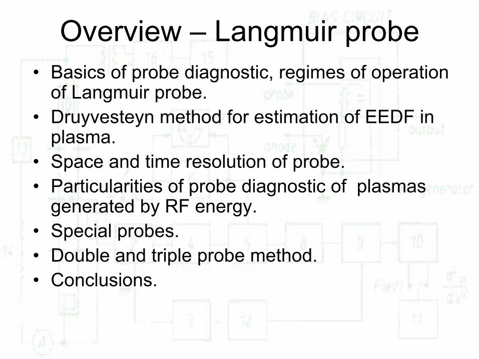
Overview – Langmuir probe• Basics of probe diagnostic, regimes of operation
of Langmuir probe.• Druyvesteyn method for estimation of EEDF in
plasma.• Space and time resolution of probe.• Particularities of probe diagnostic of plasmas
generated by RF energy.• Special probes.• Double and triple probe method.• Conclusions.
Overview – mass-spectrometry
• Principles of mass-spectrometers.• Detectors for mass-spectrometers.• Application of mass-spectrometry for
diagnostic of low-temperature plasmas.• Mass-spectra interpretation, examples,
methods PTR-MS and EA-MS.• Conclusions.
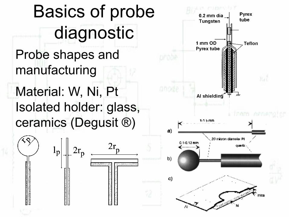
Basics of probe diagnostic
Probe shapes and manufacturing
Material: W, Ni, PtIsolated holder: glass, ceramics (Degusit ®)
Basics of probe diagnostic
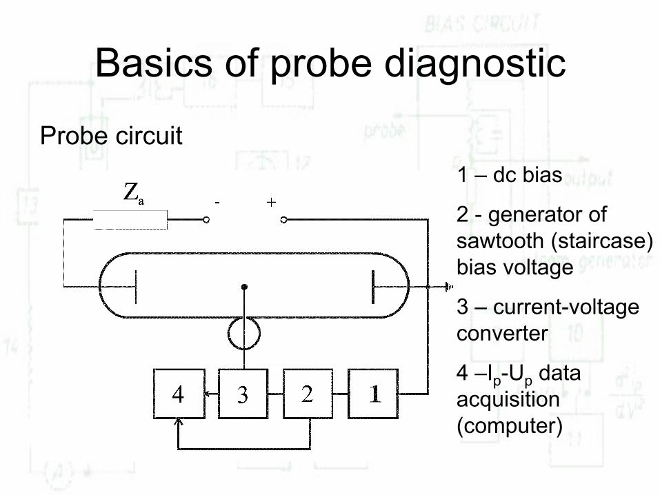
Probe circuit1 – dc bias
2 - generator of sawtooth (staircase) bias voltage
3 – current-voltage converter
4 –Ip-Up data acquisition (computer)
Basics of probe diagnostic
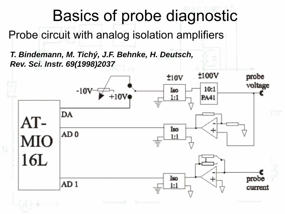
T. Bindemann, M. Tichý, J.F. Behnke, H. Deutsch, Rev. Sci. Instr. 69(1998)2037
Probe circuit with analog isolation amplifiers
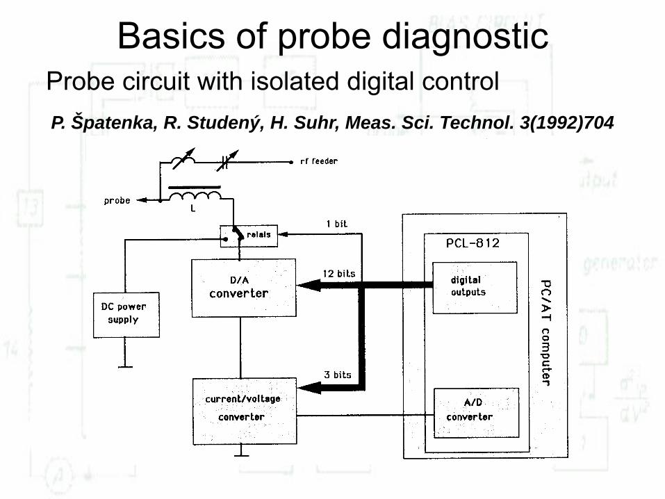
Basics of probe diagnostic
P. Špatenka, R. Studený, H. Suhr, Meas. Sci. Technol. 3(1992)704
Probe circuit with isolated digital control
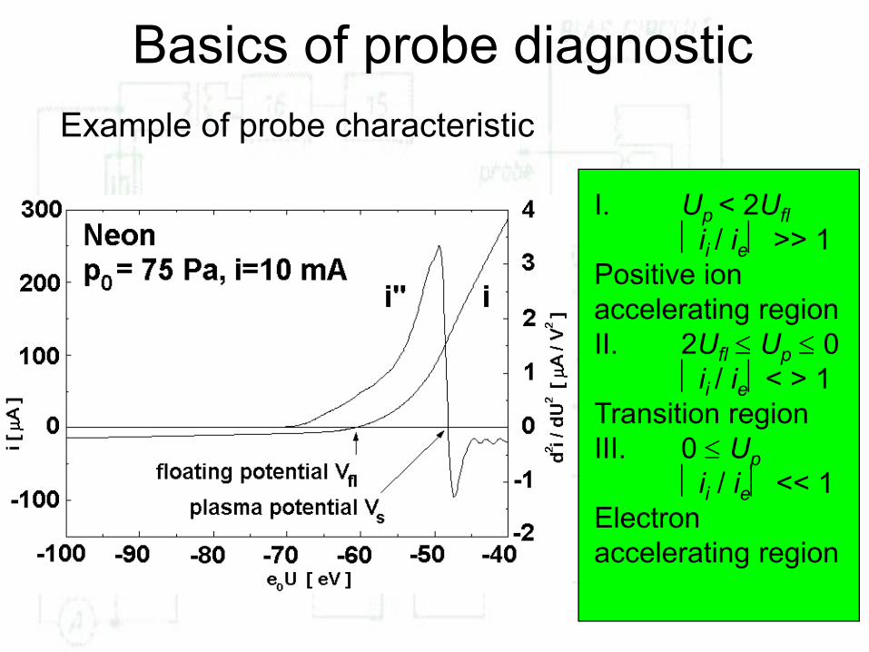
Basics of probe diagnosticExample of probe characteristic
I. Up < 2Ufl⏐ii / ie⏐ >> 1
Positive ion accelerating regionII. 2Ufl ≤ Up ≤ 0
⏐ii / ie⏐< > 1Transition regionIII. 0 ≤ Up
⏐ii / ie⏐ << 1Electron accelerating region
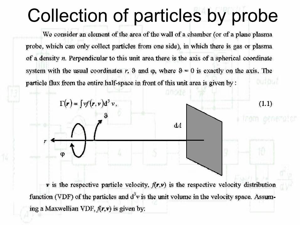
Collection of particles by probe
Collection of particles by probe

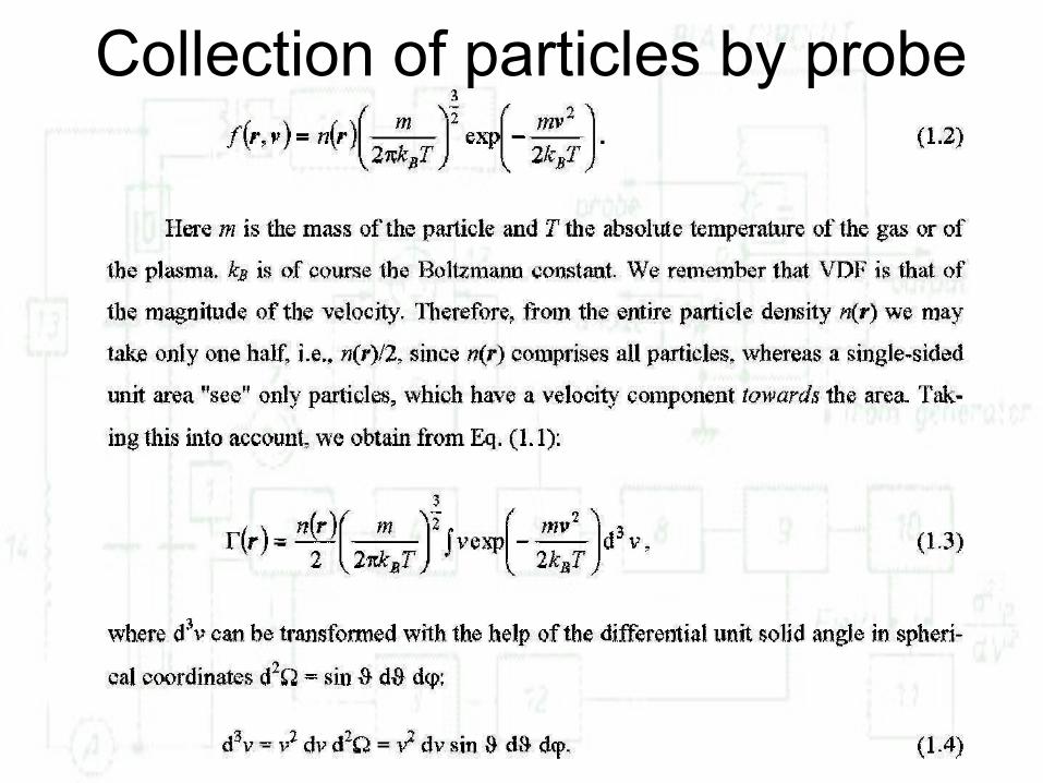
Collection of particles by probe
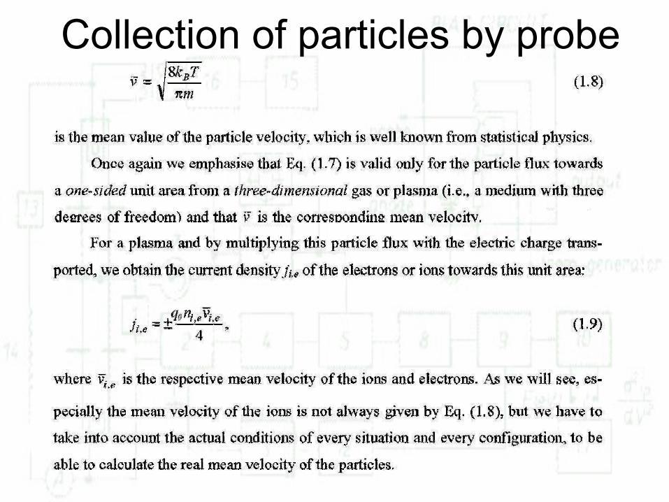
Collection of particles by probe

Working regimes of Langmuir probe
e
eBD nq
Tk20
0ελ =
Parameters:•Characteristic probe dimension rp,•Mean free path for ions, electrons, λi, λe,•Debye shielding length λD,•Degree of plasma anisothermicity τ =Te / Ti.
The thickness of the probe sheath is of the order of several λD‘s.We distinguish the following working regimes:
1. λi,e >> rp >> λD Collision-free movement of charge carriers in thin sheath (space charge limit).
2. λi,e >> λD >> rp Collision-free movement of charge carriers in thick sheath (orbital motion limit, OML).
3. λD >> λi,e >> rp Probe current is determined by collisions of charged and neutral particles in space-charge sheath around the probe.
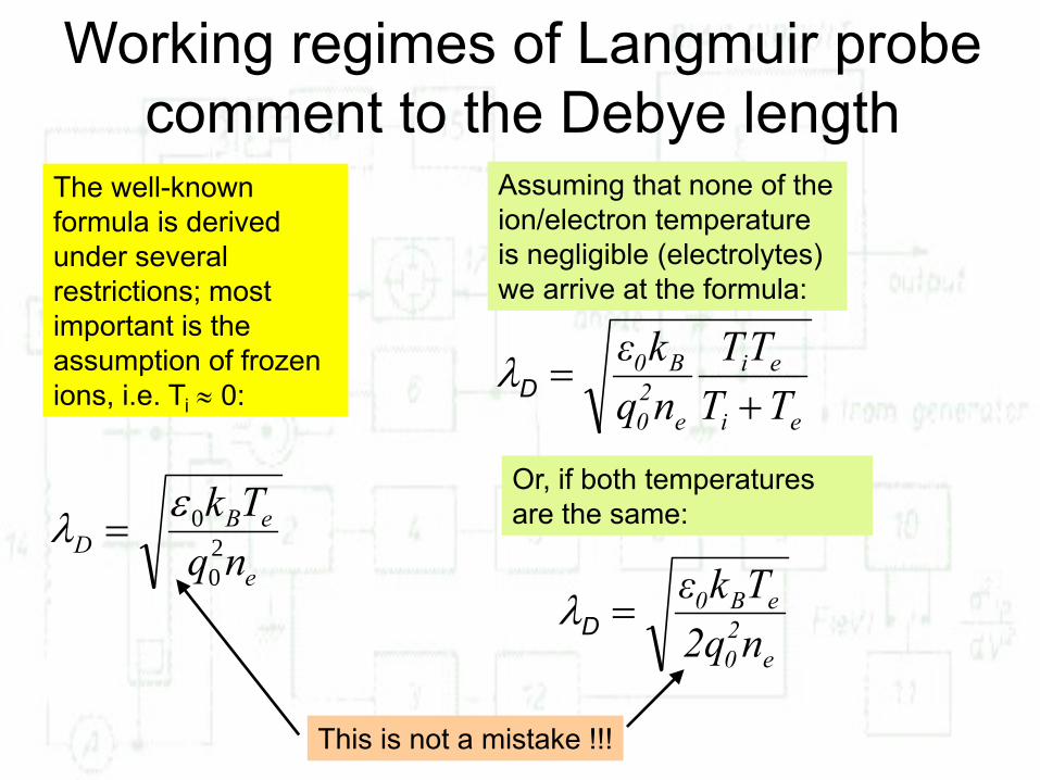
This is not a mistake !!!
Working regimes of Langmuir probecomment to the Debye length
e
eBD nq
Tk20
0ελ =
The well-known formula is derived under several restrictions; most important is the assumption of frozen ions, i.e. Ti ≈ 0:
ei
ei
e20
B0
TTTT
nqkε
+=Dλ
Assuming that none of the ion/electron temperature is negligible (electrolytes) we arrive at the formula:
Or, if both temperatures are the same:
e20
eB0
n2qTkε
=Dλ
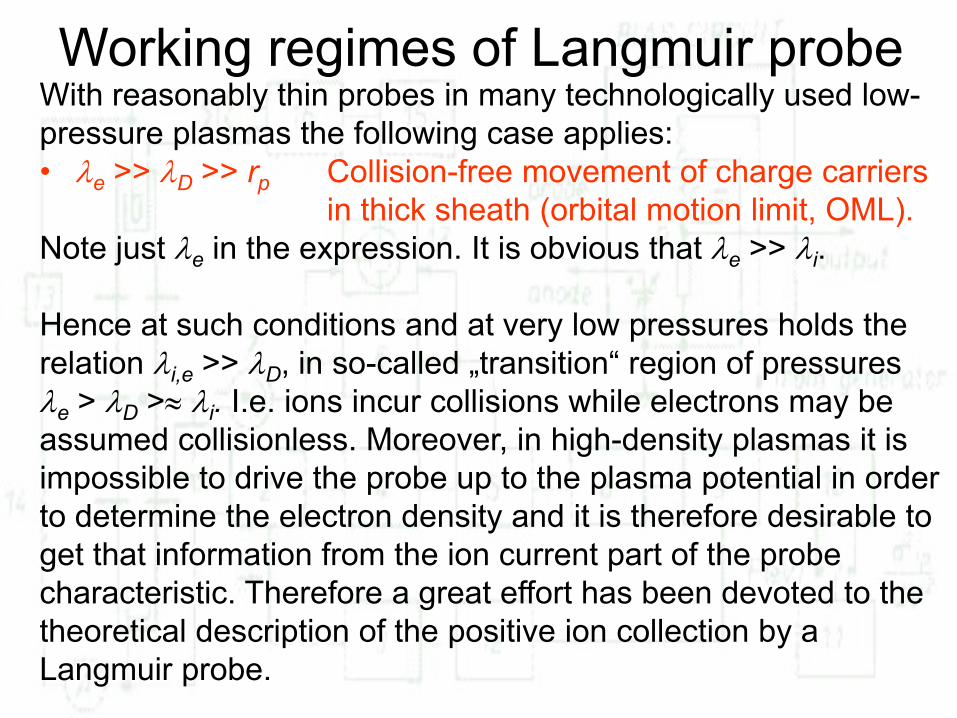
Working regimes of Langmuir probeWith reasonably thin probes in many technologically used low-pressure plasmas the following case applies: • λe >> λD >> rp Collision-free movement of charge carriers
in thick sheath (orbital motion limit, OML).Note just λe in the expression. It is obvious that λe >> λi.
Hence at such conditions and at very low pressures holds therelation λi,e >> λD, in so-called „transition“ region of pressuresλe > λD >≈ λi. I.e. ions incur collisions while electrons may beassumed collisionless. Moreover, in high-density plasmas it isimpossible to drive the probe up to the plasma potential in orderto determine the electron density and it is therefore desirable toget that information from the ion current part of the probecharacteristic. Therefore a great effort has been devoted to thetheoretical description of the positive ion collection by aLangmuir probe.
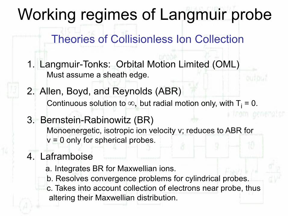
Theories of Collisionless Ion Collection
1. Langmuir-Tonks: Orbital Motion Limited (OML)Must assume a sheath edge.
2. Allen, Boyd, and Reynolds (ABR)Continuous solution to ∞, but radial motion only, with Ti = 0.
3. Bernstein-Rabinowitz (BR)Monoenergetic, isotropic ion velocity v; reduces to ABR for v = 0 only for spherical probes.
4. Laframboisea. Integrates BR for Maxwellian ions. b. Resolves convergence problems for cylindrical probes.c. Takes into account collection of electrons near probe, thusaltering their Maxwellian distribution.
Working regimes of Langmuir probe
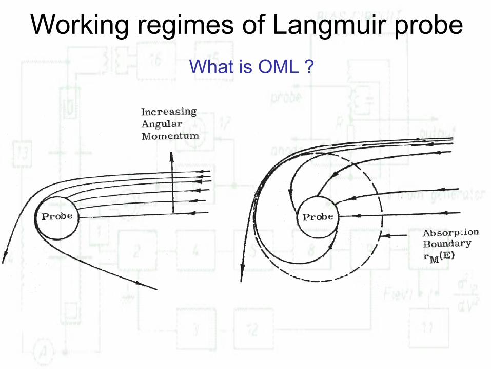
Working regimes of Langmuir probeWhat is OML ?

Working regimes of Langmuir probeCOLLISIONLESS CASE
NON-ISOTHERMAL PLASMATi<TeBohm criterion – probe potential is screened only to kBTe/2q0. Consequence: the positive ions get accelerated in the pre-sheath and the ion current is determined by Te. Anisothermicity parameter τ=Te/Tiis introduced. For the purpose of theoretical calculations the probe current and voltage is normalised:
ine,
ie,*ie, II
I =( )
eB
pp Tk
VVq 00 −=η
D. Bohm, E.H.S. Burhop, H.S.W. Massey, The Characteristics of Electrical Discharges in Magnetic Fields, A. Guthrie, R.K. Wakerling, Eds., (McGraw-Hill, New York 1949) p.77.
21
ie,
eBpie,0ine, m2
TkAnqI ⎟⎟⎠
⎞⎜⎜⎝
⎛=
π
Working regimes of Langmuir probe
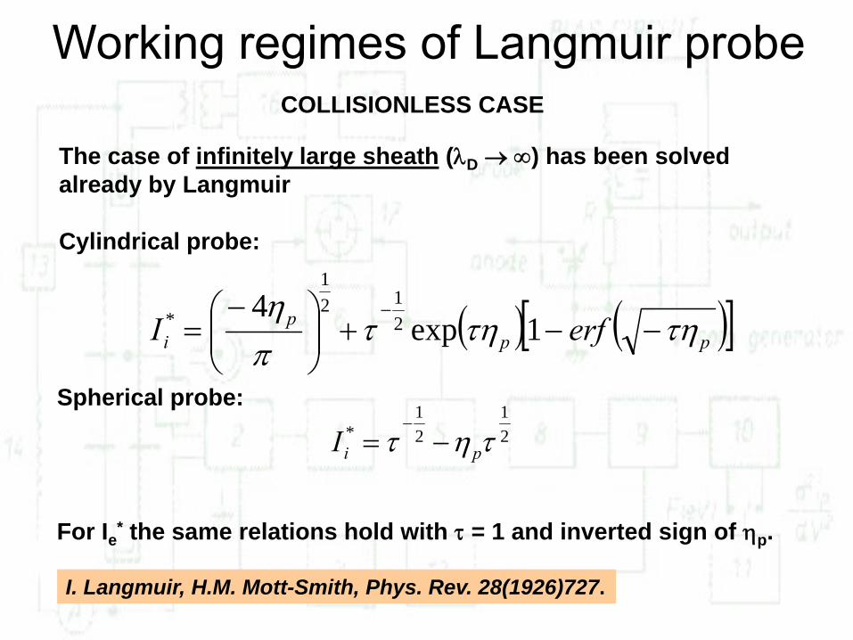
The case of infinitely large sheath (λD → ∞) has been solved already by Langmuir
Cylindrical probe:
( ) ( )[ ]ppp
i erfI τητητπη
−−+⎟⎟⎠
⎞⎜⎜⎝
⎛ −=
−1exp
4212
1
*
Spherical probe:21
21
* τητ piI −=−
For Ie* the same relations hold with τ = 1 and inverted sign of ηp.
COLLISIONLESS CASE
I. Langmuir, H.M. Mott-Smith, Phys. Rev. 28(1926)727.
Working regimes of Langmuir probeCOLLISIONLESS CASE
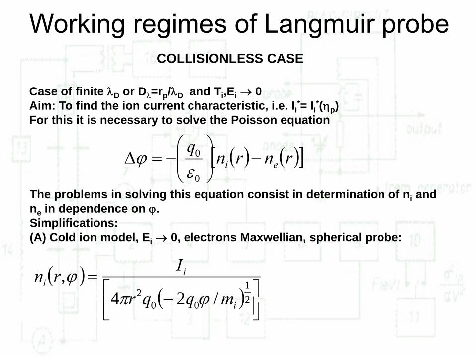
Case of finite λD or Dλ=rp/λD and Ti,Ei → 0Aim: To find the ion current characteristic, i.e. Ii*= Ii*(ηp)For this it is necessary to solve the Poisson equation
( ) ( )[ ]rnrnqei −⎟⎟
⎠
⎞⎜⎜⎝
⎛−=Δ
0
0
εϕ
The problems in solving this equation consist in determination of ni and ne in dependence on ϕ.Simplifications:(A) Cold ion model, Ei → 0, electrons Maxwellian, spherical probe:
( )( ) ⎥⎦
⎤⎢⎣⎡ −
=21
002 /24
,i
ii
mqqr
Irnϕπ
ϕ
Working regimes of Langmuir probeCOLLISIONLESS CASE
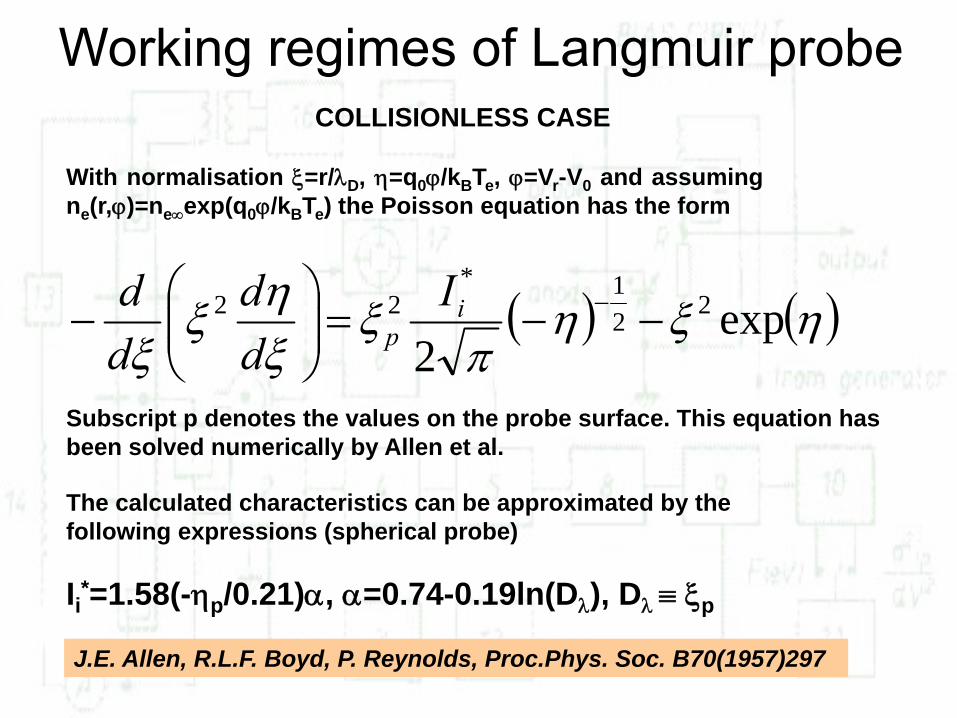
With normalisation ξ=r/λD, η=q0ϕ/kBTe, ϕ=Vr-V0 and assumingne(r,ϕ)=ne∞exp(q0ϕ/kBTe) the Poisson equation has the form
( ) ( )ηξηπ
ξξηξ
ξexp
222
1*22 −−=⎟⎟
⎠
⎞⎜⎜⎝
⎛− −i
pI
dd
dd
Subscript p denotes the values on the probe surface. This equation has been solved numerically by Allen et al.
J.E. Allen, R.L.F. Boyd, P. Reynolds, Proc.Phys. Soc. B70(1957)297
The calculated characteristics can be approximated by the following expressions (spherical probe)
Ii*=1.58(-ηp/0.21)α, α=0.74-0.19ln(Dλ), Dλ ≡ ξp

Working regimes of Langmuir probeCOLLISIONLESS CASE
Absorption radius
Allen, Boyd, Reynolds theory: radial motion theory (does not assume orbital motion)
Radial motion theory of cylindrical probe has been treated by Chen. The calculated characteristics can again be approximated by analytical formulae; practical expressions were derived by
S. Klagge, DSc dissertation, EMA UNI Greifswald, 1988 Ii*=a(-ηp/b)α with a=(Dλ+0.6)0.05+0.04, b=0.09[exp(1/Dλ)+0.08]α=(Dλ+3.1)-0.6
Formulae are valid for 0.25<Dλ<100, 0.5<ηp<50.F.F. Chen, Plasma Phys. 7(1965)47
probe

Working regimes of Langmuir probeCOLLISIONLESS CASE
B) Case of finite λD or Dλ=rp/λD and Ei > 0
spherical probe, monoenergetic ionsI.B. Bernstein, I. Rabinowitz, Phys. Fluids 2(1959)112
spherical and cylindrical probe, Ei monoenergetic and Ei MaxwellianJ.G. Laframboise, UTIAS Report 100(1966)(sometimes referred to as BRL theory)
For cylindrical probe and Ei>0, however, Ii*(Laframboise)<Ii*(Chen)
Reason for this sometimes called Chen-Laframboise paradoxon lies in different assumption of the charged particle angular momentum distribution far from the probe: (Laframboise – isotropic, ABR-Chen - δ function)
The more general model for Ei>0 (electrons Maxwellian) has been developed byJ.I. Fernández Palop, J. Ballesteros, V. Colomer, M.A. Hernández, J. Phys. D: Appl. Phys. 29(1996)2832This model includes the ABR-Chen model for Ei=0 as a special case.
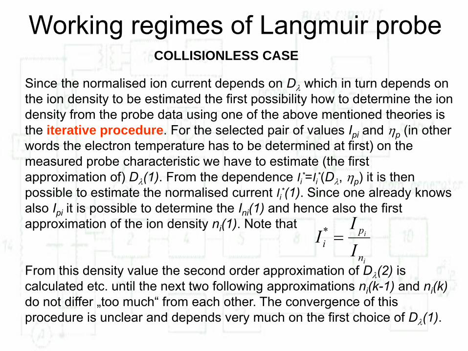
Since the normalised ion current depends on Dλ which in turn depends on the ion density to be estimated the first possibility how to determine the ion density from the probe data using one of the above mentioned theories is the iterative procedure. For the selected pair of values Ipi and ηp (in other words the electron temperature has to be determined at first) on the measured probe characteristic we have to estimate (the first approximation of) Dλ(1). From the dependence Ii*=Ii*(Dλ, ηp) it is then possible to estimate the normalised current Ii*(1). Since one already knows also Ipi it is possible to determine the Ini(1) and hence also the first approximation of the ion density ni(1). Note that
From this density value the second order approximation of Dλ(2) is calculated etc. until the next two following approximations ni(k-1) and ni(k)do not differ „too much“ from each other. The convergence of this procedure is unclear and depends very much on the first choice of Dλ(1).
Working regimes of Langmuir probeCOLLISIONLESS CASE
i
i
n
p*i II
I =
Working regimes of Langmuir probeCOLLISIONLESS CASE
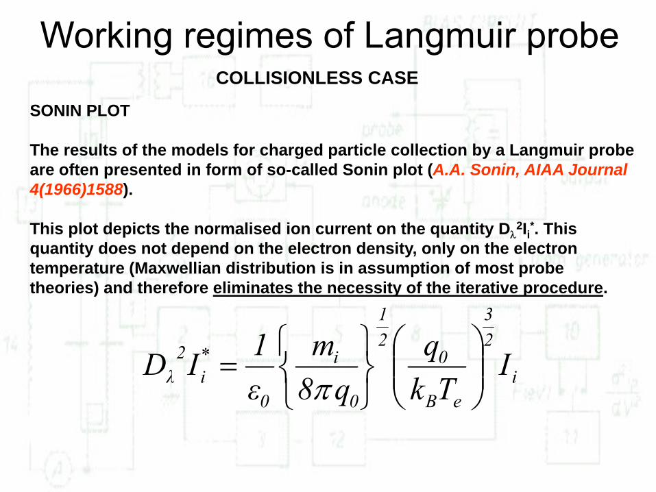
SONIN PLOT
The results of the models for charged particle collection by a Langmuir probe are often presented in form of so-called Sonin plot (A.A. Sonin, AIAA Journal 4(1966)1588).
This plot depicts the normalised ion current on the quantity Dλ2Ii*. This
quantity does not depend on the electron density, only on the electron temperature (Maxwellian distribution is in assumption of most probe theories) and therefore eliminates the necessity of the iterative procedure.
i
23
eB
021
0
i
0
*i
2λ I
Tkq
q8m
ε1ID ⎟⎟
⎠
⎞⎜⎜⎝
⎛
⎭⎬⎫
⎩⎨⎧
=π
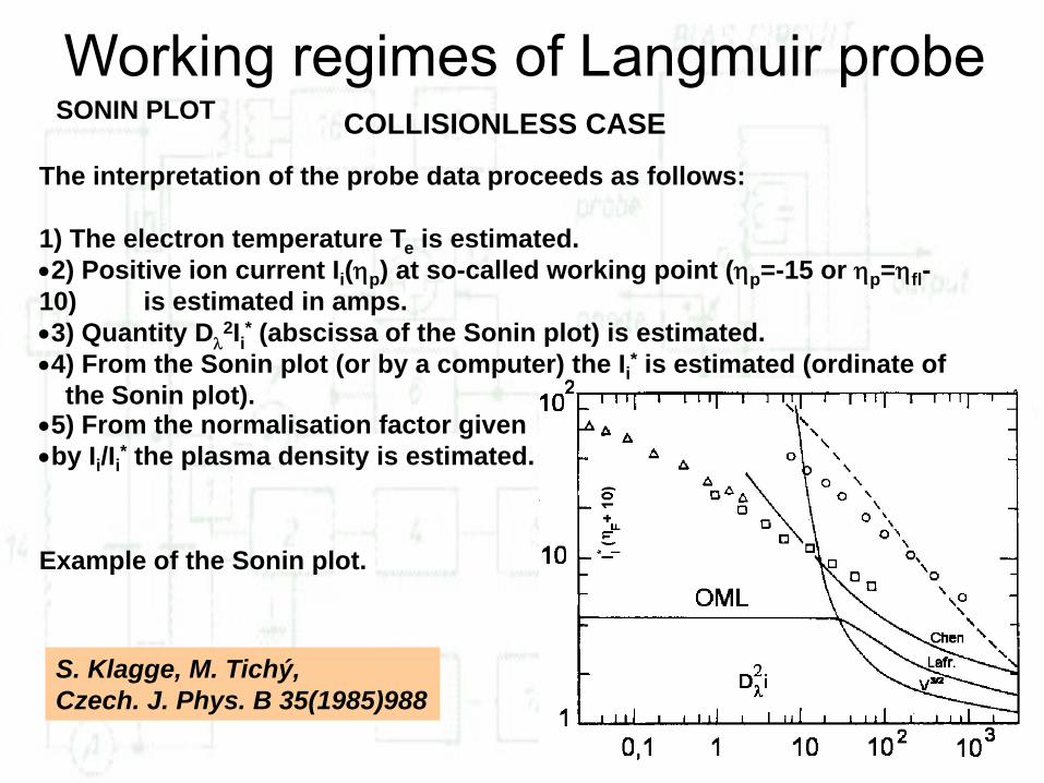
Working regimes of Langmuir probeCOLLISIONLESS CASESONIN PLOT
The interpretation of the probe data proceeds as follows:
1) The electron temperature Te is estimated.•2) Positive ion current Ii(ηp) at so-called working point (ηp=-15 or ηp=ηfl-10) is estimated in amps.•3) Quantity Dλ
2Ii* (abscissa of the Sonin plot) is estimated.•4) From the Sonin plot (or by a computer) the Ii* is estimated (ordinate of
the Sonin plot).
Example of the Sonin plot.
S. Klagge, M. Tichý, Czech. J. Phys. B 35(1985)988
•5) From the normalisation factor given •by Ii/Ii* the plasma density is estimated.
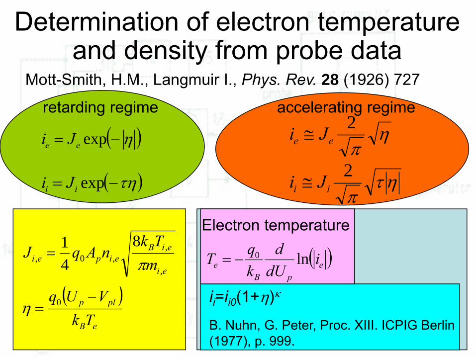
Determination of electron temperature and density from probe data
ei
eiBeipei m
TknAqJ
,
,,0,
841
π=
( )eB
plp
TkVUq −
= 0η
ηπ2
ee Ji ≅
ητπ2
ii Ji ≅
Mott-Smith, H.M., Langmuir I., Phys. Rev. 28 (1926) 727
retarding regime accelerating regime
( )η−= expee Ji
( )τη−= expii Ji
B. Nuhn, G. Peter, Proc. XIII. ICPIG Berlin (1977), p. 999.
ii=ii0(1+η)κ
Electron temperature
( )epB
e idUd
kqT ln0−=
Determination of electron temperature and density from probe data
When determining the electron temperature we have to keep in mind that we measure the SUM of electron and positive ion currents. While for the determination of Te we need the slope of the semilogarithmic plot of ie only. The original procedure how to eliminate ii consists in linear extrapolation of ii using the „saturated“ part of the probe characteristic back to plasma potential. However, except in the case of spherical probe we do no have theoretical basis for linear extrapolation. For the double-logarithmic approximation using the Nuhn and Peter formula we need to know the Tesince the formula uses probe potential normalized to Te (and, in addition, knowledge of the plasma potential is also necessary).The way out offers the use of second derivative of the probe characteristics with respect to the probe potential; if it is possible to obtain it either directly by measurement or off-line using numerical differentiation. Since the derivative of an exponential function is again exponential function, the slope in semilogarithmic scale of the second derivative yields immediately the electron temperature.
Determination of electron temperature and density from probe data
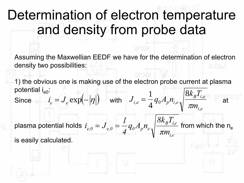
Assuming the Maxwellian EEDF we have for the determination of electron density two possibilities:
1) the obvious one is making use of the electron probe current at plasma potential ie0:Since with at
plasma potential holds from which the ne
is easily calculated.
( )η−= expee Jiei
eiBeipei m
TknAqJ
,
,,0,
841
π=
ei,
ei,Bep0e,0e,0 πm
T8knAq
41Ji ==

Determination of electron temperature and density from probe data
2) Provided that we are able to measure in the electron accerating region (typically in the afterglow plasma, but also in lower density active plasma) and that the OML model for electrons holds, we can estimate the ne from
so-called i2 vs V plot. Since in this region we arrive at the following expression for ie2:
The i2 vs V plot is therefore linear and its slope yields the (squared) electron density. Note that in this method we need to estimate neither the electron temperature nor the plasma potential prior to this procedure. However, especially in dense plasmas we are unable to measure within enough voltage range into the electron accelerating region.
ηπ2
ee Ji ≅
( )plpe
2
2e
2p
302
e VUmπnAq
2i −=
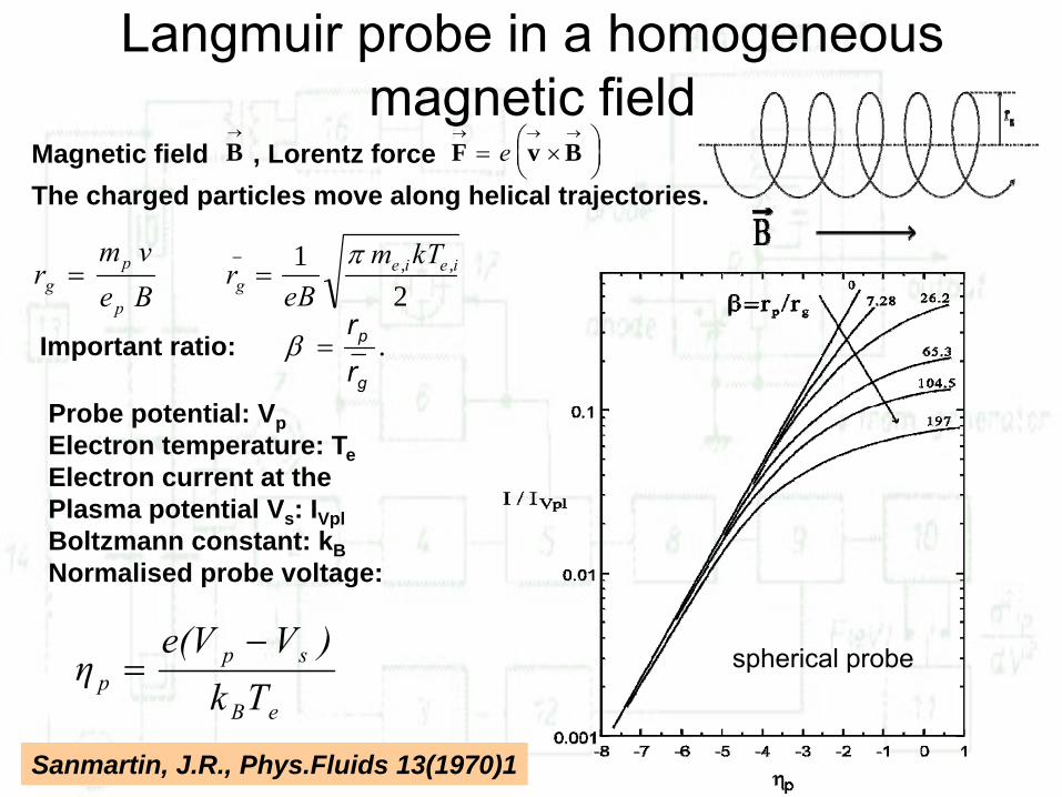
Magnetic field , Lorentz force
Langmuir probe in a homogeneous magnetic field
B→
F v B→ → →
= ×⎛⎝⎜
⎞⎠⎟
e
The charged particles move along helical trajectories.
rm ve Bgp
p
= reB
m kTg
e i e i_
, ,=1
2π
Sanmartin, J.R., Phys.Fluids 13(1970)1
Important ratio: ._g
p
rr
=β
eB
spp Tk
)Ve(Vη
−=
Probe potential: VpElectron temperature: TeElectron current at the Plasma potential Vs: IVplBoltzmann constant: kBNormalised probe voltage:
spherical probe

Langmuir probe in a homogeneous magnetic field
Cylindrical probe; infinitely large λD
Laframboise, J.G., Rubinstein, J., Phys. Fluids 19(1976)1900
Important parameter: angle Θ between the probe axis and the vector of the magnetic field
Consequence: Effect of magnetic field on the probe is smallest when the probe is oriented perpendicular to magnetic field.
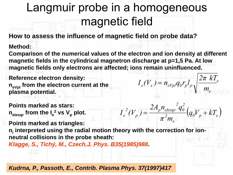
Langmuir probe in a homogeneous magnetic field
How to assess the influence of magnetic field on probe data?
Kudrna, P., Passoth, E., Contrib. Plasma Phys. 37(1997)417
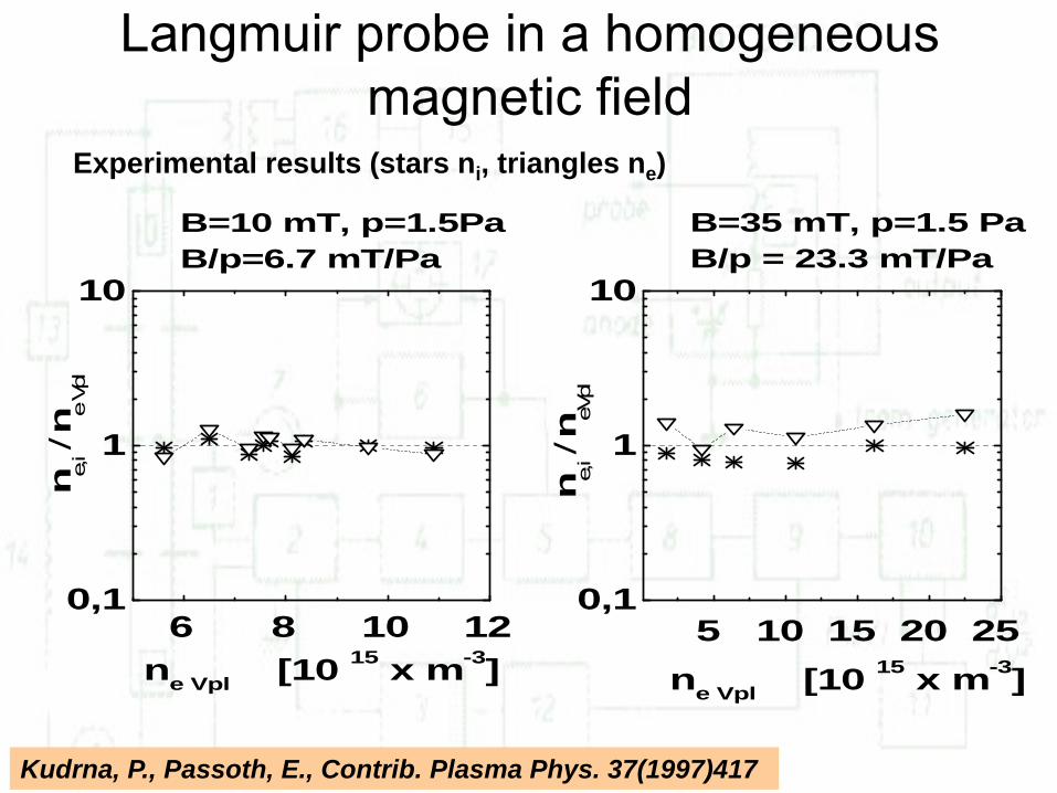
Method: Comparison of the numerical values of the electron and ion density at different magnetic fields in the cylindrical magnetron discharge at p=1,5 Pa. At low magnetic fields only electrons are affected; ions remain uninfluenced.
e
epp0eVplse m
kT2πlrqn)(VI =Reference electron density:neVpl from the electron current at the plasma potential.
( )ep0e
2
20
2eIesqrp
p2e kTVq
mπqn2A
)(VI +=Points marked as stars:neIesqr from the Ie2 vs Vp plot.
Points marked as triangles: ni interpreted using the radial motion theory with the correction for ion-neutral collisions in the probe sheath: Klagge, S., Tichý, M., Czech.J. Phys. B35(1985)988.
Langmuir probe in a homogeneous magnetic field
Experimental results (stars ni, triangles ne)
Kudrna, P., Passoth, E., Contrib. Plasma Phys. 37(1997)417
5 10 15 20 250,1
1
10
B=35 mT, p=1.5 PaB/p = 23.3 mT/Pa
B=10 mT, p=1.5PaB/p=6.7 mT/Pa
n e,i / n
eVpl
ne Vpl [10 15 x m-3]
6 8 10 120,1
1
10
n e,i / n
e Vp
l
ne Vpl [10 15 x m-3]

Druyvesteyn method for determination of EEDF in plasma M.J. Druyvesteyn, Z. Physik 64(1930)781
( ) 121
0
=∫∞
ppp duuuf
( )ppeep
e ufAnmqdUid 2
1
23
23
02
2
2
−=
pp
ep
p
ee dU
dUidU
Am
qn ∫
∞
⎟⎟⎠
⎞⎜⎜⎝
⎛=
02
2212
123
0
2
pp
ep
pp
ep
m
dUdUidU
dUdUidUq
uq
2
2
0
21
2
2
0
23
0
0
∫
∫∞
∞
=
Druyvesteyn method for determination of EEDF in plasma
The second derivative necessary for the estimation of the EEDF can be either directly measured (on-line methods) or computed numerically from the experimental data (off-line methods).
Experimental set-ups for on-line measurement of the second derivative of the total probe current work on following principles:
- use of the non-linearity of the probe characteristic, i.e. the relation between the „curvature“ of the characteristic and second harmonic generation [G.R. Branner, E.M. Friar, G. Medicus, Rev. Sci. Instr. 34(1963)231], mixing [S.C.M. Luijendijk, J. Van Eck, Physica 36(1967)49], detection of the modulated signal [N.A. Vorobjeva, J.M. Kagan, V.M. Milenin, Zhurnal tekhnicheskoi fiziki (J.Tech.Phys. USSR) 34(1964)2079] etc.,- direct analog differentiators using operational amplifiers and sawtooth-like probe voltage [V.A. Godyak, R.B. Piejak, B.M. Alexandrovich, Plasma Sources Sci. Technol. 1(1992)36],- analog difference amplifiers and stepwise-like probe voltage [B. Saggau, Zeitschrift für angewandte Physik 32(1972)324].
Druyvesteyn method for determination of EEDF in plasma
The off-line differentiating methods are either based on algorithms of the numerical analysis or on direct numeric solution of the integral equation [L.M. Volkova, A.M. Devyatov, G.A. Kralkina, N.N. Sedov, M.A. Sherif: Vestnik Mosk.Univ.(fizika, astronomija) 16(1957)502]
or on the non-recursive digital filtering of a dependence given as a set of data [M. Hannemann, INP-Report VII. Institute for Low-Temperature Plasma Physics, Greifswald, 1995, D. Trunec, Contrib. Plasma Phys. 32(1992)523, J.I. Fernández Palop, J. Ballesteros, V. Colomer, M.A. Hernández, Rev. Sci. Instr. 66(1995)4625].
It is important to note that the Druyvesteyn formula includes second derivative of just electron current. To replace the electron by the total probe current is permissible only when the ion current can be approximated by linear relation. Since that is not always the case the residual influence of the second derivative of the ion current leads to lower dynamics of the estimated EEDF (2-3 orders of magnitude compared to 4 orders of magnitude when Ii“ is eliminated.

Druyvesteyn method for determination of EEDF in plasma
The most common procedure for differentiation of noisy experimental data is the „sliding polynomial approximation“. This represents approximation of the selected odd number M=2m+1 (m=1,2,...) adjacent data points around selected xl by a second order polynomial p(x)=a0+a1x+a2x2 (for xl-m*h ≤ x ≤ xl+m*h). The second derivative at xl is hence
Since the coefficient a2 is a weighted sum of the ordinates yi(for l-m ≤ i ≤ l+m) this method may be regarded as the digital filtering where the weights are the filter coefficients ci / (h2). Tables of such coefficients are given by Savitzky and Golay [i] and formulae for the evaluation of these filter coefficients in [ii]. Computer programs that make use of this procedure have already been constructed and reported [iii].
[i] A. Savitzky, M.J.E. Golay, Anal. Chem. 36(1964)1627.[ii] H. Madden, Anal. Chem. 50(1978)1383.[iii] M. Tichý, P. Kudrna, J.F. Behnke, C. Csambal, S. Klagge,
Journal de Physique IV France 7(1997)C4-397.
( ) ( )y x al2
0 22=

Druyvesteyn method for determination of EEDF in plasma
In all procedures for the estimation of the second derivative of the probe characteristic the second derivative is estimated not from the infinitesimally small vicinity of the point where the derivative is estimated, but from the finite voltage (energy) interval around this point. This leads to a distortion of the estimated second derivative in comparison with the theoretical one. It
can be shown [i] that the estimated second derivative is related to the theoretical one via convolution with so-called apparatus
function :
T ≠ 0 only within
( )′′I up
( )′′I up( )T u up p− ′
( ) ( ) ( ) ppppp uduuTuIuI ′′−′′′′=′′ ∫+∞
∞−
A typical course of the apparatus function (case of the second harmonic procedure [ii]) is
[i] H. Amemyia, J.Appl.Phys. 15(1976)1767.[ii] V.I. Demidov, N.B. Kolokolov, Zhurnal tekhnicheskoi fiziki (J.Tech.Phys.
USSR) 51(1981)888 (in Russian).
( )T u uu uap p
p p− ′ = −− ′⎛
⎝⎜
⎞
⎠⎟
⎛
⎝⎜⎜
⎞
⎠⎟⎟
83
12
32
π
− ≤− ′
≤1 1u ua
p p
Druyvesteyn method for determination of EEDF in plasma
Generally, one has to be careful in the choice of the degree of smoothness in any of the methods mentioned above. Secondary maximums or local deficits on the EEDF due to elementary processes that create or require electrons at a certain range of energies that do come from the nature of the investigated plasma should not be suppressed. When in doubt whether a particular irregularity on the EEDF is due to the plasma processes or due to noise the best recommendation is to process one set of data with different kinds of differentiating methods and compare the results with theoretical expectations.
Also, practice has shown that in order to get EEDF’s that are close to reality it is a better way to enhance the signal-to-noise ratio of the measured signal from the probe than to try to process numerically the data with a bad signal-to-noise ratio.
i
ipi m
nq
0
20
εω =
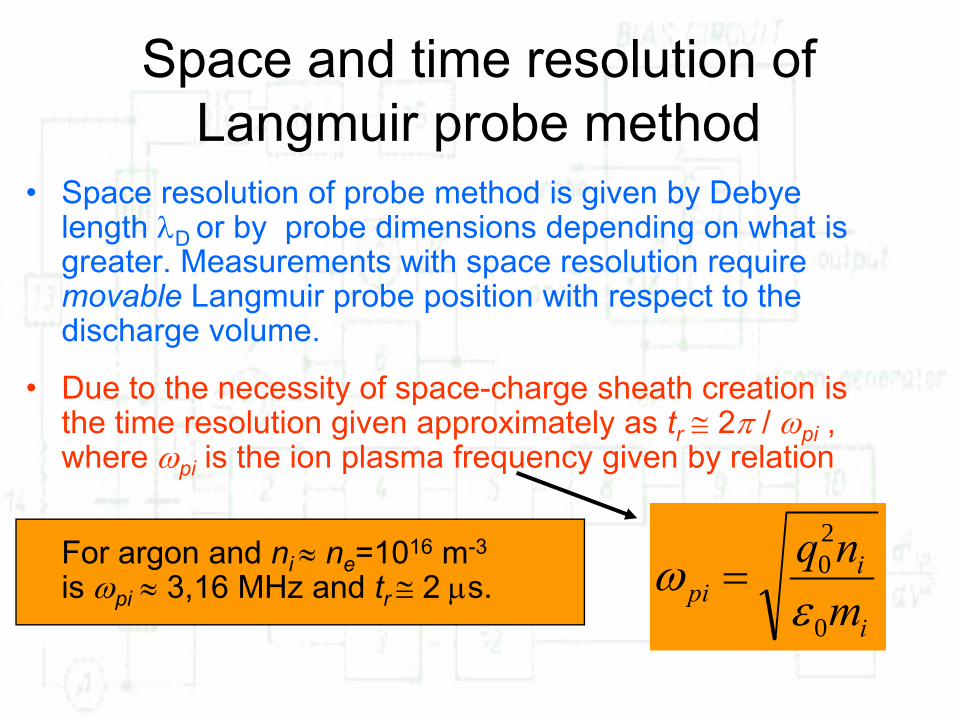
Space and time resolution of Langmuir probe method
• Space resolution of probe method is given by Debye length λD or by probe dimensions depending on what is greater. Measurements with space resolution require movable Langmuir probe position with respect to the discharge volume.
• Due to the necessity of space-charge sheath creation is the time resolution given approximately as tr ≅ 2π / ωpi , where ωpi is the ion plasma frequency given by relation
For argon and ni ≈ ne=1016 m-3
is ωpi ≈ 3,16 MHz and tr ≅ 2 μs.
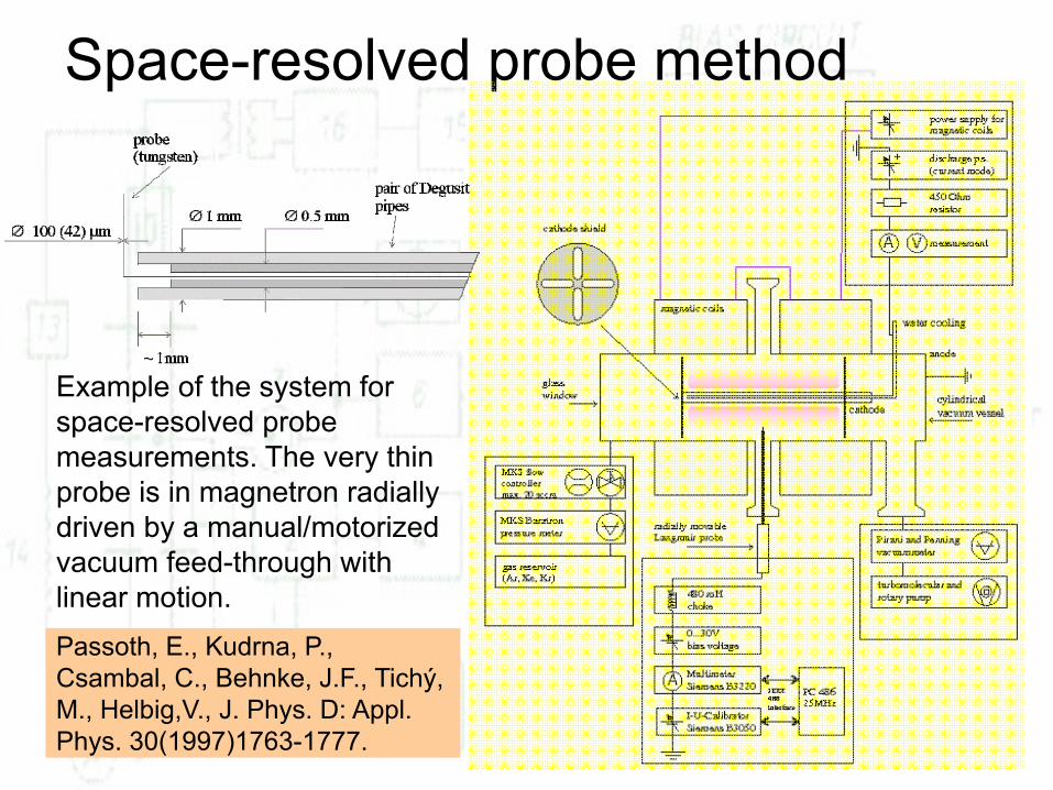
Space-resolved probe method
Example of the system for space-resolved probe measurements. The very thin probe is in magnetron radially driven by a manual/motorized vacuum feed-through with linear motion.Passoth, E., Kudrna, P., Csambal, C., Behnke, J.F., Tichý, M., Helbig,V., J. Phys. D: Appl. Phys. 30(1997)1763-1777.

Space-resolved probe method
510
15
0,20,4
0,60,8
1,0
10-3
10-2
10-1
100
f0 [ V-3/2 ]
εp [eV]x = r / R A
J.F. Behnke, E. Passoth, C. Csambal, M. Tichý, P. Kudrna, D. Trunec, A. Brablec,Czechoslovak Journal of Physics B 49(1999)483-498 .
Measured EEDF‘s in dependence on the radial coordinate. With increasing distance from the cathode to the anode the EEDF changes shape from Maxwellian with higher electron temperature to „double temperature“ EEDF with very low temperature of the EEDF body.
6 8 10 12 14 16 18 20 22 24 26 28 300
2
4
6
8
black 0o
red 45o
green 90o
E mea
n [eV
]
r [mm]
0,5
1,0
1,5
2,0
2,5
3,0
3,5
4,0
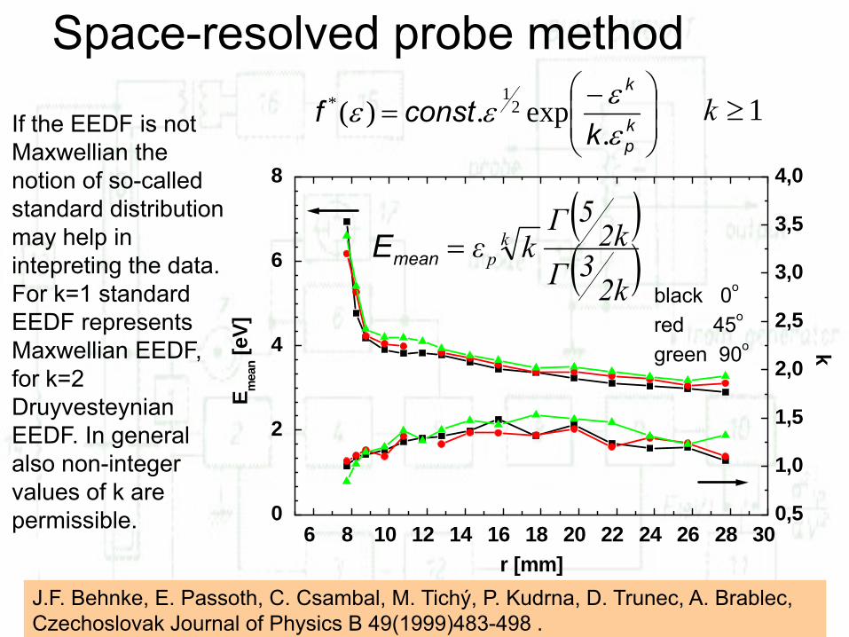
kSpace-resolved probe method
J.F. Behnke, E. Passoth, C. Csambal, M. Tichý, P. Kudrna, D. Trunec, A. Brablec,Czechoslovak Journal of Physics B 49(1999)483-498 .
⎟⎟⎠
⎞⎜⎜⎝
⎛ −= k
p
k
kconstf
εεεε.
exp.)( 21* 1≥kIf the EEDF is not
Maxwellian the notion of so-called standard distribution may help in intepreting the data. For k=1 standard EEDF represents Maxwellian EEDF, for k=2 Druyvesteynian EEDF. In general also non-integer values of k are permissible.
( )( )2k3Γ2k5Γ
kε kp=meanE
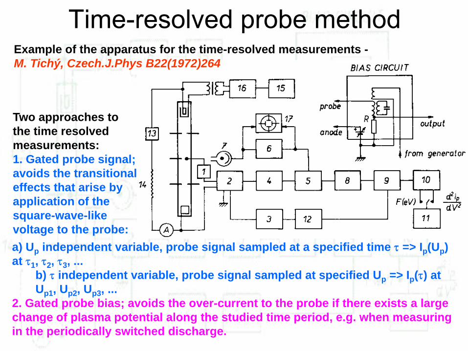
Time-resolved probe methodExample of the apparatus for the time-resolved measurements -M. Tichý, Czech.J.Phys B22(1972)264
a) Up independent variable, probe signal sampled at a specified time τ => Ip(Up) at τ1, τ2, τ3, ...
b) τ independent variable, probe signal sampled at specified Up => Ip(τ) at Up1, Up2, Up3, ...
2. Gated probe bias; avoids the over-current to the probe if there exists a large change of plasma potential along the studied time period, e.g. when measuring in the periodically switched discharge.
Two approaches to the time resolved measurements:1. Gated probe signal; avoids the transitional effects that arise by application of the square-wave-like voltage to the probe:
Direction-resolved Langmuir probe method
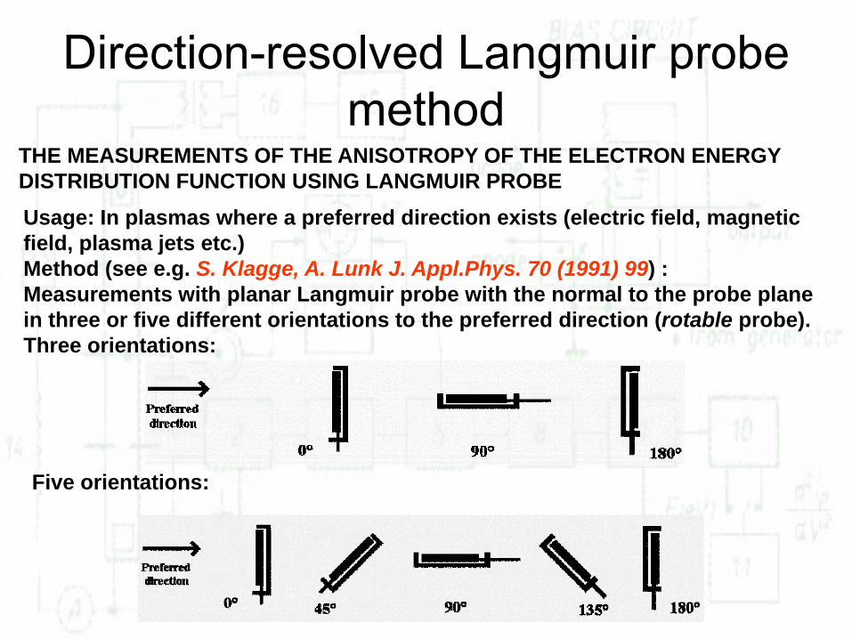
THE MEASUREMENTS OF THE ANISOTROPY OF THE ELECTRON ENERGY DISTRIBUTION FUNCTION USING LANGMUIR PROBEUsage: In plasmas where a preferred direction exists (electric field, magnetic field, plasma jets etc.)Method (see e.g. S. Klagge, A. Lunk J. Appl.Phys. 70 (1991) 99) :Measurements with planar Langmuir probe with the normal to the probe plane in three or five different orientations to the preferred direction (rotable probe).Three orientations:
Five orientations:
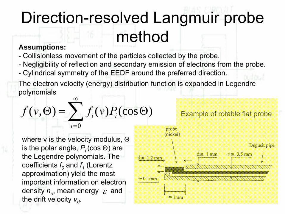
where v is the velocity modulus, Θis the polar angle, Pi (cos Θ) are the Legendre polynomials. The coefficients f0 and f1 (Lorentz approximation) yield the most important information on electron density ne, mean energy and the drift velocity vd.
Direction-resolved Langmuir probe method
Assumptions:- Collisionless movement of the particles collected by the probe.- Negligibility of reflection and secondary emission of electrons from the probe.- Cylindrical symmetry of the EEDF around the preferred direction.The electron velocity (energy) distribution function is expanded in Legendre polynomials
∑∞
=
Θ=Θ0
)(cos)(),(i
ii Pvfvf
ε
Example of rotable flat probe
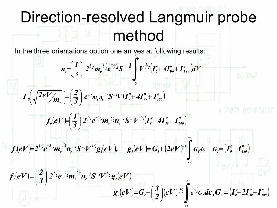
In the three orientations option one arrives at following results:
Direction-resolved Langmuir probe method
( )∫∞
−′′+′′+′′−⎟
⎠⎞
⎜⎝⎛=
0
18090021
23
21e
21
e dVII4IV1Sem231n
( )18090011
ee2
e0 II4IVSe3
2m2eVF nm ′′+′′+′′= −−−
⎟⎟⎠
⎞⎜⎜⎝
⎛⎟⎠
⎞⎜⎝
⎛
( ) ( )1809002111
e21e
25
21
o II4IVSnme231eVf ′′+′′+′′= −−−
⎟⎟⎠
⎞⎜⎜⎝
⎛
( ) ( ) ( ) ( ) ∫∞
−−−− +==eV
11
1112111
e
21
e25
21
1 dεG2eVGeVg,eVgVSnme2eVf ( )18001 IIG ′′−′′=
( ) ( )eVgVSnme232eVf 2
2111
e21
e25
21
2−−−
⎟⎟⎠
⎞⎜⎜⎝
⎛=
( ) ( ) ( )18090022
eV
21
23
22 II2IG,dεeV23GeVg Gε ′′+′′−′′=+= ∫
∞
−
⎟⎟⎠
⎞⎜⎜⎝
⎛
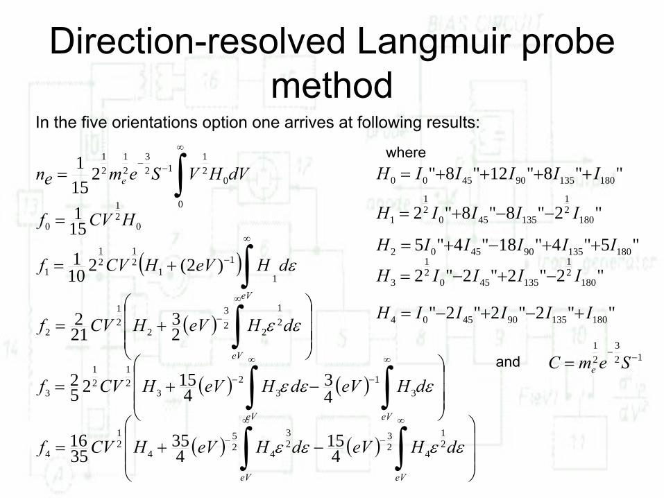
In the five orientations option one arrives at following results:
Direction-resolved Langmuir probe method
dVHVSemen e 0
0
21
123
21
21
2151 ∫
∞
−−=
021
0 151 HCVf =
( )∫∞
−+=
eV
dHeVHCVf ε1
11
21
21
1 )2(2101
( )⎟⎟⎟
⎠
⎞
⎜⎜⎜
⎝
⎛+= ∫
∞
−
eV
dHeVHCVf εε 21
223
221
2 23
212
( ) ( )⎟⎟⎟
⎠
⎞
⎜⎜⎜
⎝
⎛−+= ∫∫
∞
−
∞
−
eVeV
dHeVdHeVHCVf εεε 31
32
321
21
3 43
41525
2
( ) ( )⎟⎟⎟
⎠
⎞
⎜⎜⎜
⎝
⎛−+= ∫∫
∞
−
∞
−
eVeV
dHeVdHeVHCVf εεεε 21
423
23
425
421
4 415
435
3516
""8"12"8" 180135904500 IIIIIH ++++=
"2"8"8"2 18021
13545021
1 IIIIH −−+=
"5"4"18"4"5 180135904502 IIIIIH ++−+=
"2"2"2"2 18021
13545021
3 IIIIH −+−=
""2"2"2" 180135904504 IIIIIH +−+−=
and 123
21
−−= SemC e
where
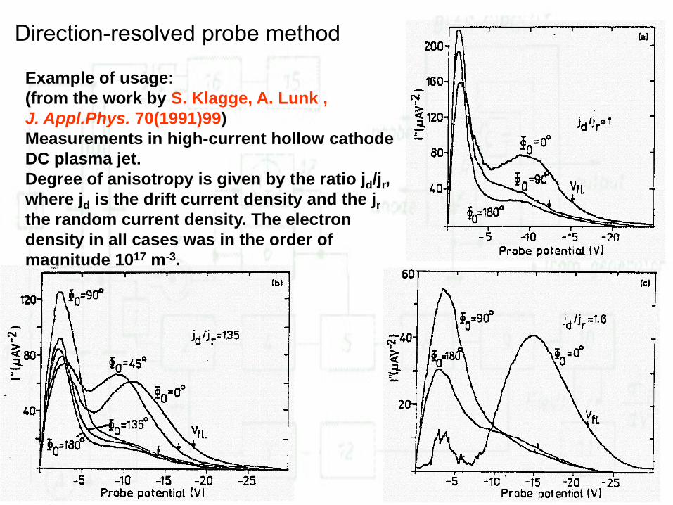
Direction-resolved probe method
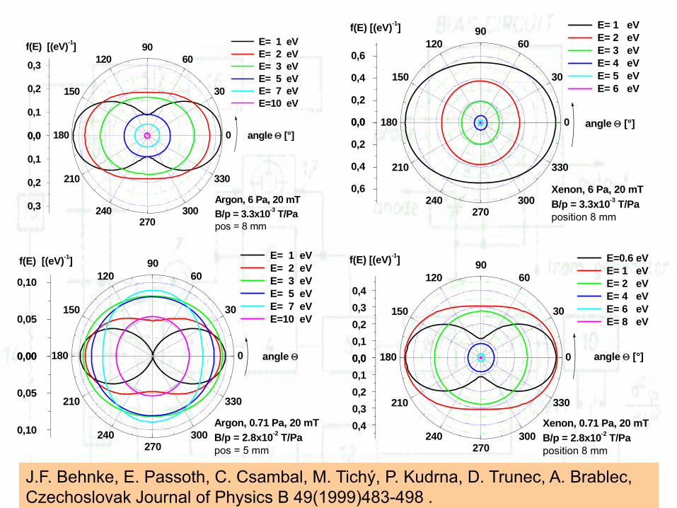
Example of usage:(from the work by S. Klagge, A. Lunk , J. Appl.Phys. 70(1991)99)Measurements in high-current hollow cathode DC plasma jet. Degree of anisotropy is given by the ratio jd/jr, where jd is the drift current density and the jrthe random current density. The electron density in all cases was in the order of magnitude 1017 m-3.
0,00,10,20,30,4
0
30
6090
120
150
180
210
240270
300
330
0,00,10,20,30,4
angle Θ [°]
f(E) [(eV)-1]
Xenon, 0.71 Pa, 20 mTB/p = 2.8x10⁻² T/Paposition 8 mm
E=0.6 eV E= 1 eV E= 2 eV E= 4 eV E= 6 eV E= 8 eV
0,0
0,2
0,4
0,6
0
30
6090
120
150
180
210
240270
300
330
0,0
0,2
0,4
0,6 Xenon, 6 Pa, 20 mTB/p = 3.3x10⁻³ T/Paposition 8 mm
f(E) [(eV)-1]
angle Θ [°]
E= 1 eV E= 2 eV E= 3 eV E= 4 eV E= 5 eV E= 6 eV
0,0
0,1
0,2
0,3
0
30
6090
120
150
180
210
240270
300
330
0,0
0,1
0,2
0,3
angle Θ [°]
f(E) [(eV)-1] E= 1 eV E= 2 eV E= 3 eV E= 5 eV E= 7 eV E=10 eV
Argon, 6 Pa, 20 mTB/p = 3.3x10⁻³ T/Papos = 8 mm
0,00
0,05
0,10
0
30
6090
120
150
180
210
240270
300
330
0,00
0,05
0,10
f(E) [(eV)-1]
angle Θ
E= 1 eV E= 2 eV E= 3 eV E= 5 eV E= 7 eV E=10 eV
Argon, 0.71 Pa, 20 mTB/p = 2.8x10⁻² T/Papos = 5 mm
J.F. Behnke, E. Passoth, C. Csambal, M. Tichý, P. Kudrna, D. Trunec, A. Brablec,Czechoslovak Journal of Physics B 49(1999)483-498 .
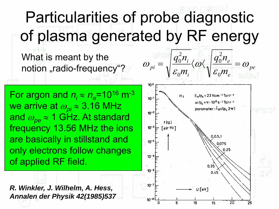
Particularities of probe diagnostic of plasma generated by RF energy
pee
e
i
ipi m
nqmnq ω
εω
εω =⟨⟨=
0
20
0
20What is meant by the
notion „radio-frequency“?
For argon and ni ≈ ne=1016 m-3
we arrive at ωpi ≈ 3.16 MHzand ωpe ≈ 1 GHz. At standard frequency 13.56 MHz the ions are basically in stillstand and only electrons follow changes of applied RF field.
R. Winkler, J. Wilhelm, A. Hess, Annalen der Physik 42(1985)537
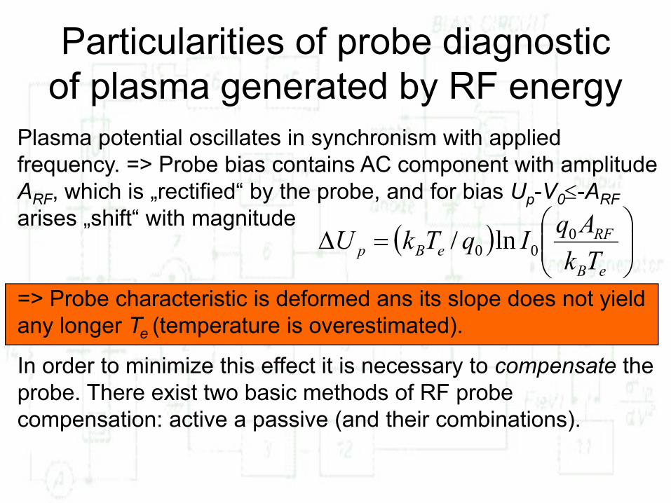
Plasma potential oscillates in synchronism with applied frequency. => Probe bias contains AC component with amplitude ARF, which is „rectified“ by the probe, and for bias Up-V0≤-ARFarises „shift“ with magnitude
=> Probe characteristic is deformed ans its slope does not yield any longer Te (temperature is overestimated).
In order to minimize this effect it is necessary to compensate the probe. There exist two basic methods of RF probe compensation: active a passive (and their combinations).
Particularities of probe diagnostic of plasma generated by RF energy
( ) ⎟⎟⎠
⎞⎜⎜⎝
⎛=Δ
eB
RFeBp Tk
AqIqTkU 000 ln/
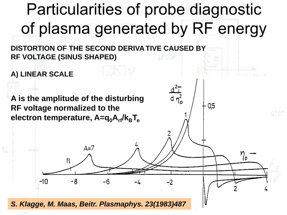
Particularities of probe diagnostic of plasma generated by RF energy
DISTORTION OF THE SECOND DERIVA TIVE CAUSED BY RF VOLTAGE (SINUS SHAPED)
A) LINEAR SCALE
S. Klagge, M. Maas, Beitr. Plasmaphys. 23(1983)487
A is the amplitude of the disturbing RF voltage normalized to the electron temperature, A=q0Arf/kBTe

Particularities of probe diagnostic of plasma generated by RF energy
DISTORTION OF THE SECOND DERIVA TIVE CAUSED BY RF VOLTAGE (SINUS SHAPED)
A) SEMILOGARITHMIC SCALE
H. Sabadil, S. Klagge, M. Kammayer, Plasma Chemistry and Plasma Processing 8(1988)425
Since ΔUp is constant with respect to η, RF distortion does not affect Te if estimated from the slope of second derivative of electron current.
The second derivatives at different A‘s have been shifted correspondingly along the voltage axis so that their slopes overlap overeach other.
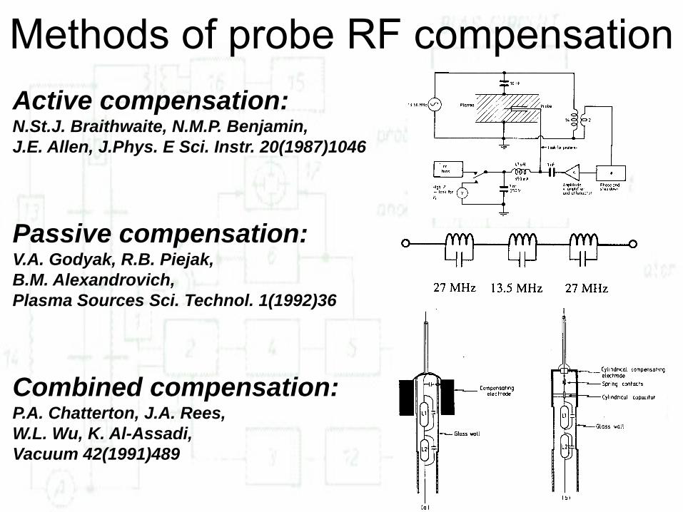
Methods of probe RF compensationActive compensation:N.St.J. Braithwaite, N.M.P. Benjamin, J.E. Allen, J.Phys. E Sci. Instr. 20(1987)1046
Passive compensation:V.A. Godyak, R.B. Piejak, B.M. Alexandrovich, Plasma Sources Sci. Technol. 1(1992)36
Combined compensation:P.A. Chatterton, J.A. Rees, W.L. Wu, K. Al-Assadi, Vacuum 42(1991)489
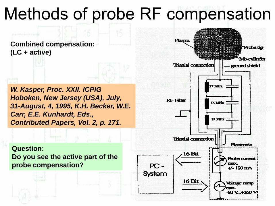
Methods of probe RF compensation
W. Kasper, Proc. XXII. ICPIG Hoboken, New Jersey (USA), July, 31-August, 4, 1995, K.H. Becker, W.E. Carr, E.E. Kunhardt, Eds., Contributed Papers, Vol. 2, p. 171.
Combined compensation:(LC + active)
Question:Do you see the active part of the probe compensation?

Methods of probe RF compensationCombined compensation (RC circuits+LC circuits+ active):
U. Flender, B.H. Nguyen Thi, K. Wiesemann, N.A. Khromov, N.B. Kolokolov, Plasma Sources Sci. Technol. 5(1996)61
Note: This method requires larger DC power supply for probe bias since a large resistor is inserted into the probe current path.
Advantage of this method consists in the fact that it is a broadband RF compensation.
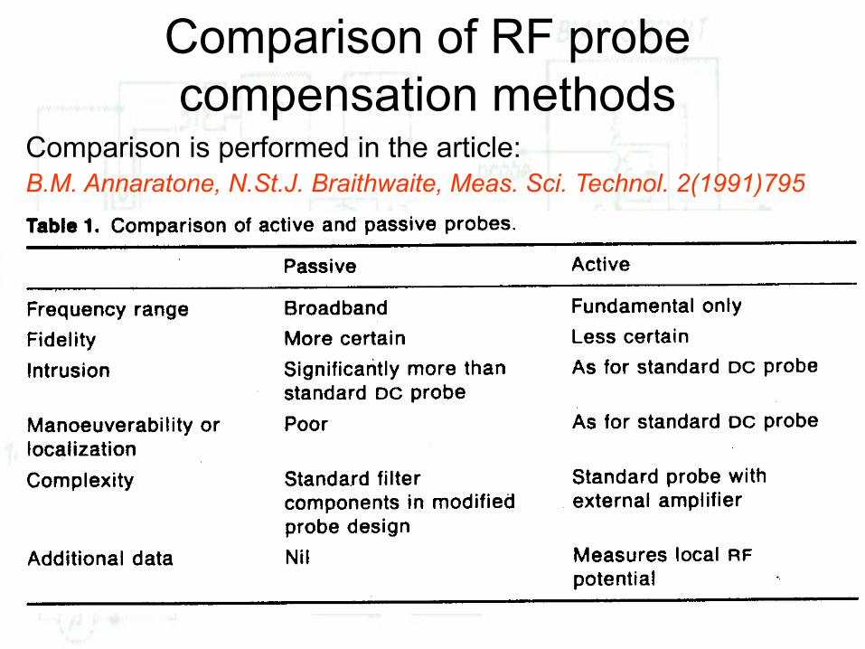
Comparison of RF probecompensation methods
Comparison is performed in the article:B.M. Annaratone, N.St.J. Braithwaite, Meas. Sci. Technol. 2(1991)795
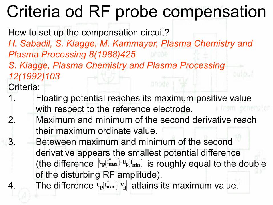
Criteria od RF probe compensationHow to set up the compensation circuit?H. Sabadil, S. Klagge, M. Kammayer, Plasma Chemistry and Plasma Processing 8(1988)425S. Klagge, Plasma Chemistry and Plasma Processing 12(1992)103Criteria:1. Floating potential reaches its maximum positive value
with respect to the reference electrode.2. Maximum and minimum of the second derivative reach
their maximum ordinate value.3. Beteween maximum and minimum of the second
derivative appears the smallest potential difference (the difference is roughly equal to the doubleof the disturbing RF amplitude).
4. The difference attains its maximum value.
⎛ ⎞ ⎛ ⎞⎜ ⎟ ⎜ ⎟⎝ ⎠ ⎝ ⎠
−" "U I U Ip max p min
⎛ ⎞⎜ ⎟⎝ ⎠
−"U I Vp max fl
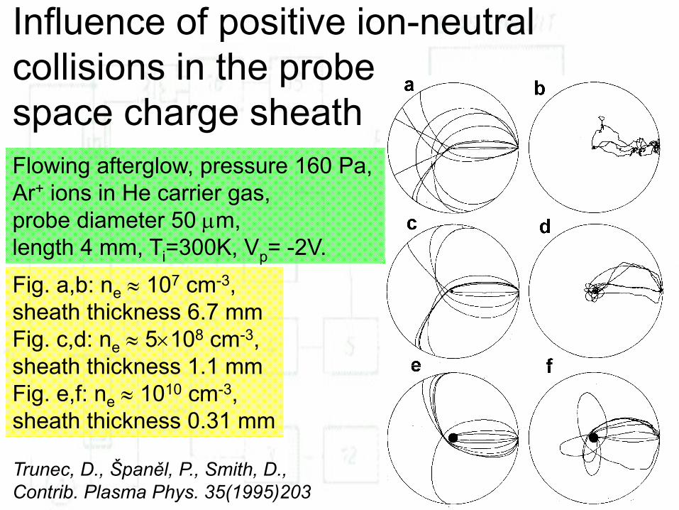
Fig. a,b: ne ≈ 107 cm-3, sheath thickness 6.7 mmFig. c,d: ne ≈ 5×108 cm-3, sheath thickness 1.1 mmFig. e,f: ne ≈ 1010 cm-3, sheath thickness 0.31 mm
Flowing afterglow, pressure 160 Pa, Ar+ ions in He carrier gas, probe diameter 50 μm, length 4 mm, Ti=300K, Vp= -2V.
Trunec, D., Španěl, P., Smith, D., Contrib. Plasma Phys. 35(1995)203
Influence of positive ion-neutral collisions in the probe space charge sheath
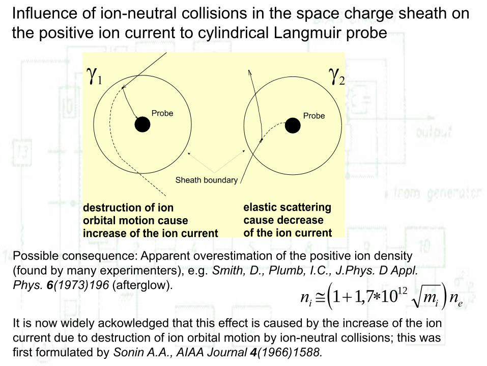
Influence of ion-neutral collisions in the space charge sheath on the positive ion current to cylindrical Langmuir probe
Possible consequence: Apparent overestimation of the positive ion density (found by many experimenters), e.g. Smith, D., Plumb, I.C., J.Phys. D Appl. Phys. 6(1973)196 (afterglow). ( )n m ni i e≅ + ∗1 1 7 1012,It is now widely ackowledged that this effect is caused by the increase of the ion current due to destruction of ion orbital motion by ion-neutral collisions; this was first formulated by Sonin A.A., AIAA Journal 4(1966)1588.

Influence of ion-neutral collisions in the space charge sheath on the positive ion current to cylindrical Langmuir probe
Quantitative assessment of the effect of orbital motion destruction has been introduced by Zakrzewski Z., Kopiczynski T., Plasma Phys. 16(1974)1195.
I Ii iL* *= ∞γ γ1 2 I I
II A kT
mnqi
ip
e
io
** , *= =where
2π
γλ1 1= +
−⎛⎝⎜
⎞⎠⎟∞ ∞
∞
I II
SiABR
iL
iL
i
* *
sheath thickness S is determined after Basu J. Sen C., Japan.J.Appl.Phys. 12(1973)1081.
Here γ1 represents the influence of the effect of orbital motion destruction (causing
the increase of the ion current) and γ2 the effect of ion scattering due to collisions
with neutrals (causing decrease of the ion current).
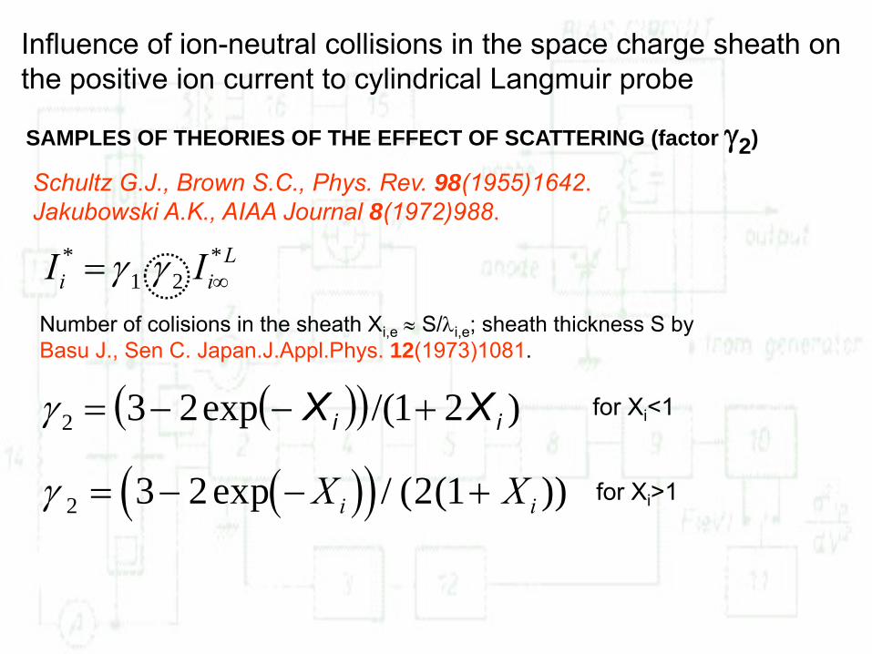
Influence of ion-neutral collisions in the space charge sheath on the positive ion current to cylindrical Langmuir probe
SAMPLES OF THEORIES OF THE EFFECT OF SCATTERING (factor γ2)
Schultz G.J., Brown S.C., Phys. Rev. 98(1955)1642.Jakubowski A.K., AIAA Journal 8(1972)988.
I Ii iL* *= ∞γ γ1 2
Number of colisions in the sheath Xi,e ≈ S/λi,e; sheath thickness S by Basu J., Sen C. Japan.J.Appl.Phys. 12(1973)1081.
( )( ) )21/(exp232 ii XX +−−=γ for Xi<1
( )( )γ 2 3 2 2 1= − − +exp / ( ( ))X Xi i for Xi>1
Influence of ion-neutral collisions in the space charge sheath on the positive ion current to cylindrical Langmuir probe
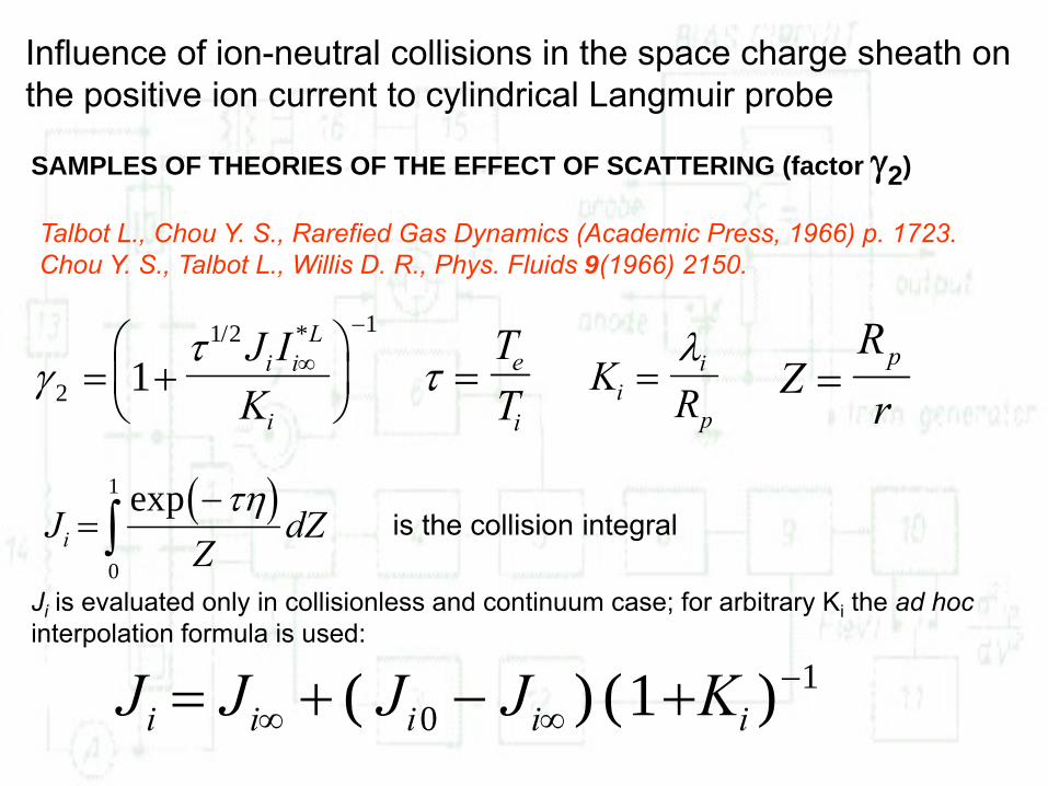
SAMPLES OF THEORIES OF THE EFFECT OF SCATTERING (factor γ2)
Talbot L., Chou Y. S., Rarefied Gas Dynamics (Academic Press, 1966) p. 1723.Chou Y. S., Talbot L., Willis D. R., Phys. Fluids 9(1966) 2150.
γτ
2
1 2 1
1= +⎛⎝⎜
⎞⎠⎟∞
−/ *J IKi i
L
iτ =
TTe
iK
Rii
p=
λ
( )JZ
dZi =−
∫exp τη
0
1
is the collision integral
ZRrp
=
Ji is evaluated only in collisionless and continuum case; for arbitrary Ki the ad hocinterpolation formula is used:
J J J J Ki i i i i= + − +∞ ∞−( ) ( )0
11
Influence of ion-neutral collisions in the space charge sheath on the positive ion current to cylindrical Langmuir probe
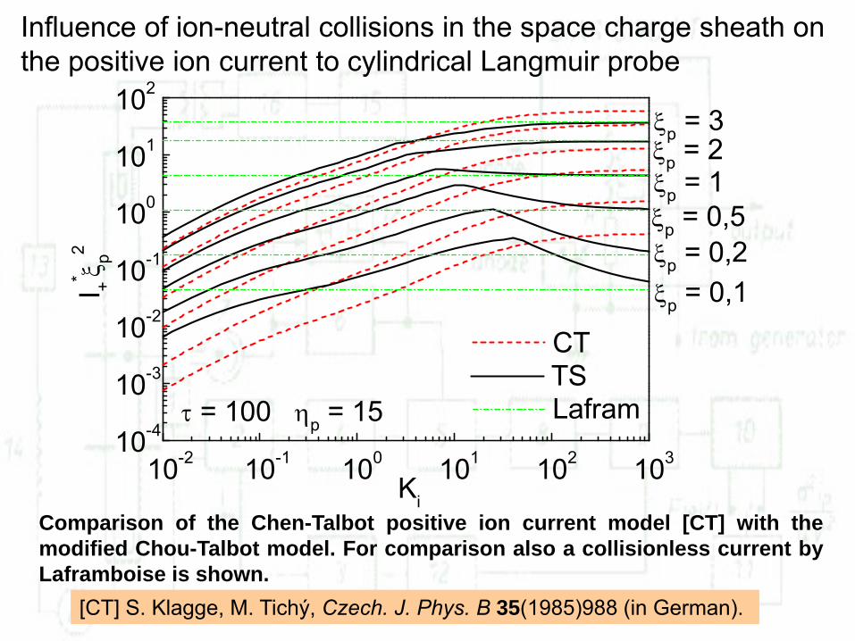
[CT] S. Klagge, M. Tichý, Czech. J. Phys. B 35(1985)988 (in German).
10-2 10-1 100 101 102 10310-4
10-3
10-2
10-1
100
101
102
CT
τ = 100 ηp = 15
I +* ξ p2
Ki
TS Lafram
ξp = 3ξp = 2ξp = 1ξp = 0,5ξp = 0,2ξp = 0,1
Comparison of the Chen-Talbot positive ion current model [CT] with themodified Chou-Talbot model. For comparison also a collisionless current byLaframboise is shown.
10-2 10-1 100 101 102 10310-4
10-3
10-2
10-1
100
101
102
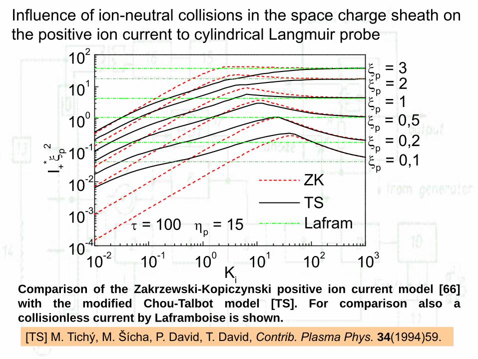
ZK
τ = 100 ηp = 15
I +* ξ p2
Ki
TS Lafram
ξp = 3ξp = 2ξp = 1ξp = 0,5ξp = 0,2ξp = 0,1
Comparison of the Zakrzewski-Kopiczynski positive ion current model [66]with the modified Chou-Talbot model [TS]. For comparison also acollisionless current by Laframboise is shown.
Influence of ion-neutral collisions in the space charge sheath on the positive ion current to cylindrical Langmuir probe
[TS] M. Tichý, M. Šícha, P. David, T. David, Contrib. Plasma Phys. 34(1994)59.

Influence of positive ion-neutral collisions in the probe space charge sheath
SUMMARYNo collisionless theory can be used to calculate the
positive ion density accurately from ion saturation currents in partially ionized plasmas.
Collisions in the presheath can destroy the ions’ angular momentum, thus increasing the ion current over the BRL value. Some orbiting still remains, however, so that ABR predicts at lower pressures (<≅1 Pa) too large a current.
At moderate pressures in active plasma the Chen-Talbot theory describes best the experimental data.

Probes in the chemically activeplasma
Problem: Distortion of the probe characteristic due to the non-conducting layer on the probe surface and/or on the reference electrode. The growth of the layer with time causes the „hysteresis“ of the probe characteristic curve. Processing of the distorted probe data by conventional methods leads to erroneous values of plasma parameters.
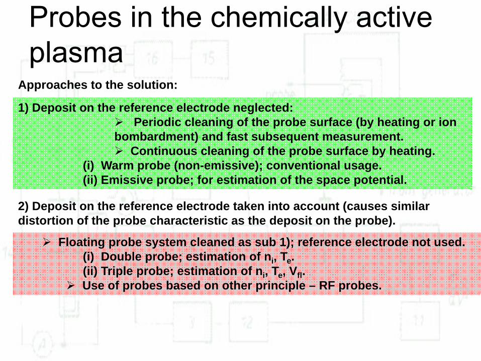
Probes in the chemically activeplasma
1) Deposit on the reference electrode neglected:Periodic cleaning of the probe surface (by heating or ion
bombardment) and fast subsequent measurement.Continuous cleaning of the probe surface by heating.
(i) Warm probe (non-emissive); conventional usage.(ii) Emissive probe; for estimation of the space potential.
Approaches to the solution:
Floating probe system cleaned as sub 1); reference electrode not used.(i) Double probe; estimation of ni, Te.(ii) Triple probe; estimation of ni, Te, Vfl.Use of probes based on other principle – RF probes.
2) Deposit on the reference electrode taken into account (causes similar distortion of the probe characteristic as the deposit on the probe).
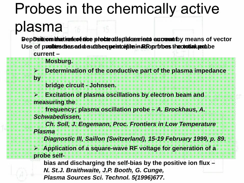
Determination of the probe displacement current by means of vectorvoltmeter and subsequent elimination from the total probe
current –Mosburg.Determination of the conductive part of the plasma impedance
bybridge circuit - Johnsen.Excitation of plasma oscillations by electron beam and
measuring thefrequency; plasma oscillation probe – A. Brockhaus, A.
Schwabedissen,Ch. Soll, J. Engemann, Proc. Frontiers in Low Temperature
Plasma Diagnostic III, Saillon (Switzerland), 15-19 February 1999, p. 89.Application of a square-wave RF voltage for generation of a
probe self-bias and discharging the self-bias by the positive ion flux –N. St.J. Braithwaite, J.P. Booth, G. Cunge, Plasma Sources Sci. Technol. 5(1996)677.
Deposit on the reference electrode taken into accountUse of probes based on other principle – RF probes - continued.
Probes in the chemically activeplasma
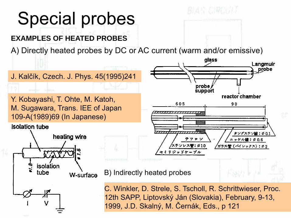
Special probesEXAMPLES OF HEATED PROBESA) Directly heated probes by DC or AC current (warm and/or emissive)
J. Kalčík, Czech. J. Phys. 45(1995)241
C. Winkler, D. Strele, S. Tscholl, R. Schrittwieser, Proc. 12th SAPP, Liptovský Ján (Slovakia), February, 9-13, 1999, J.D. Skalný, M. Černák, Eds., p 121
Y. Kobayashi, T. Ohte, M. Katoh, M. Sugawara, Trans. IEE of Japan 109-A(1989)69 (In Japanese)
B) Indirectly heated probes
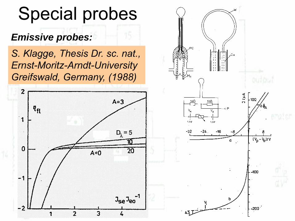
Special probes
S. Klagge, Thesis Dr. sc. nat., Ernst-Moritz-Arndt-University Greifswald, Germany, (1988)
Emissive probes:
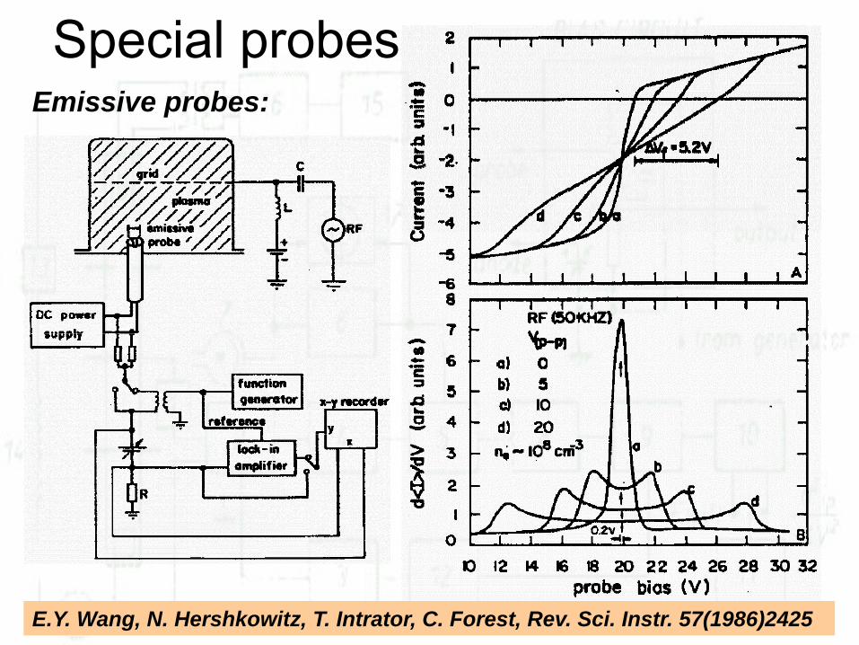
Special probesEmissive probes:
E.Y. Wang, N. Hershkowitz, T. Intrator, C. Forest, Rev. Sci. Instr. 57(1986)2425
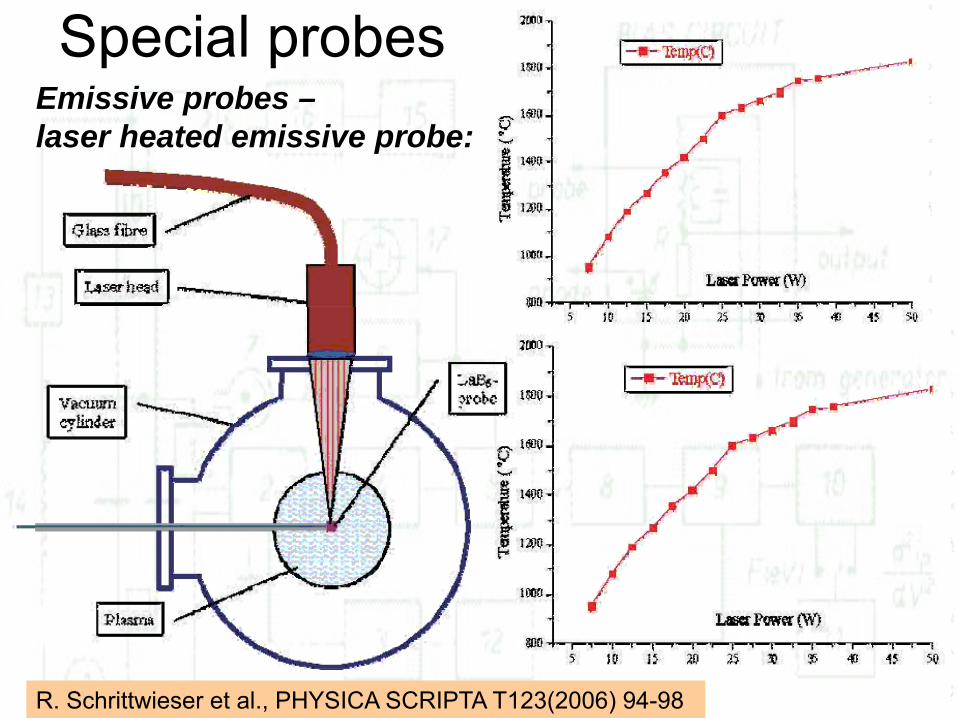
Special probesEmissive probes –laser heated emissive probe:
R. Schrittwieser et al., PHYSICA SCRIPTA T123(2006) 94-98
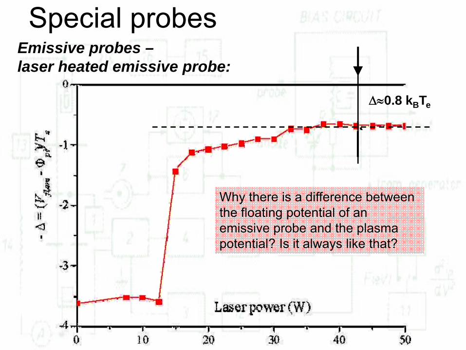
Special probesEmissive probes –laser heated emissive probe:
Δ≈0.8 kBTe
Why there is a difference between the floating potential of an emissive probe and the plasma potential? Is it always like that?

Special probesEmissive probe – creation of negative potential barrier due to emitted electrons
Schematics of formation of the potential barrier in front of the floating emitting probe.
strong emission
critical emission
weak emission
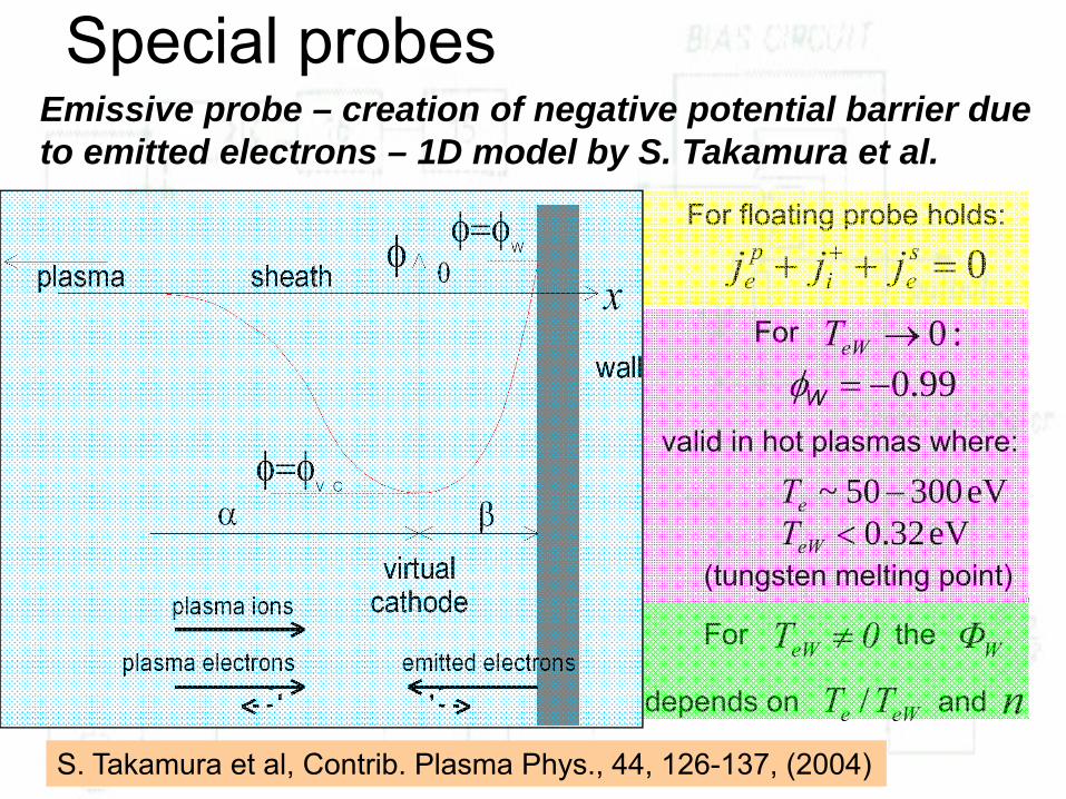
Special probesEmissive probe – creation of negative potential barrier due to emitted electrons – 1D model by S. Takamura et al.
S. Takamura et al, Contrib. Plasma Phys., 44, 126-137, (2004)
0TeW ≠
99.0−=Wφvalid in hot plasmas where:
0=++ + sei
pe jjj
For floating probe holds:
eV30050~ −eT
depends on and
eV32.0<eWT(tungsten melting point)
:0→eWTFor
For the
eWe TT / nWΦ
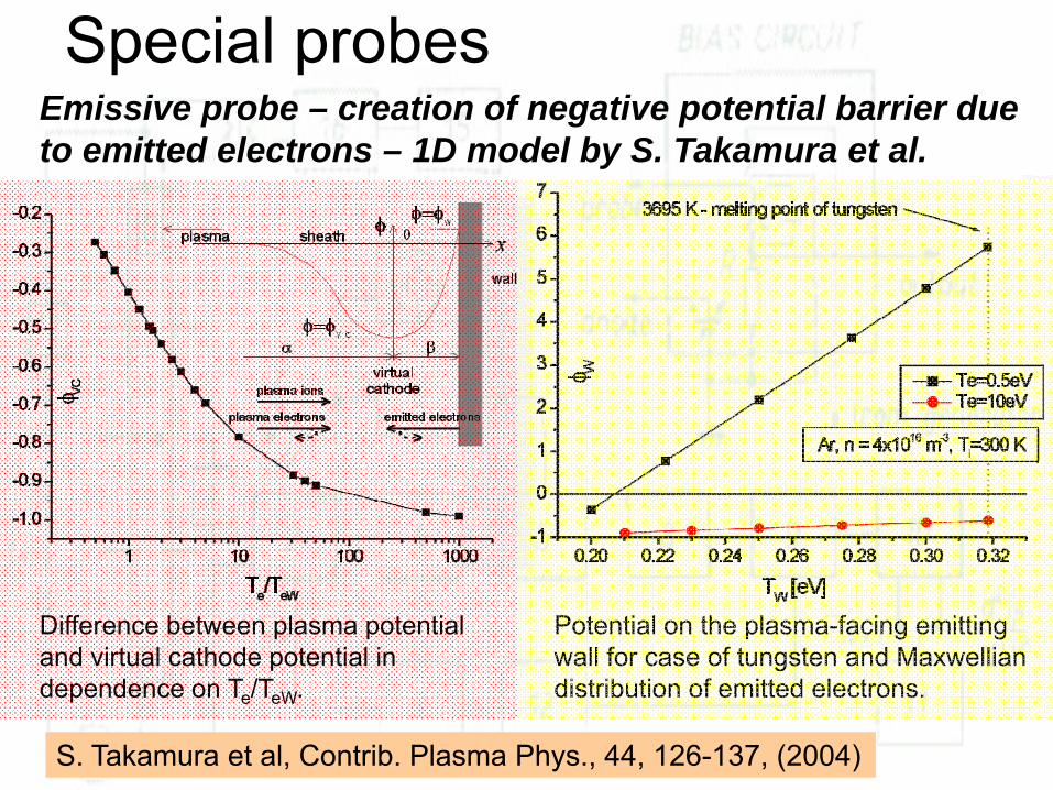
Special probesEmissive probe – creation of negative potential barrier due to emitted electrons – 1D model by S. Takamura et al.
S. Takamura et al, Contrib. Plasma Phys., 44, 126-137, (2004)
Difference between plasma potential and virtual cathode potential in dependence on Te/TeW.
Potential on the plasma-facing emitting wall for case of tungsten and Maxwellian distribution of emitted electrons.

Special probesOscillating probe:A. Brockhaus, A. Schwabedissen, Ch. Soll, J. Engemann, Proc. Frontiers in Low Temperature Plasma Diagnostic III, Saillon (Switzerland), 15-19 February 1999, p. 89
20
0
epe
e
q nm
ωε
=
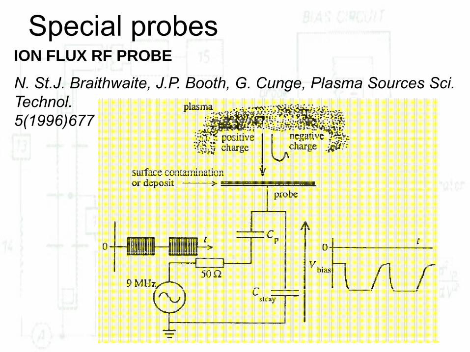
Special probesION FLUX RF PROBE
N. St.J. Braithwaite, J.P. Booth, G. Cunge, Plasma Sources Sci. Technol. 5(1996)677
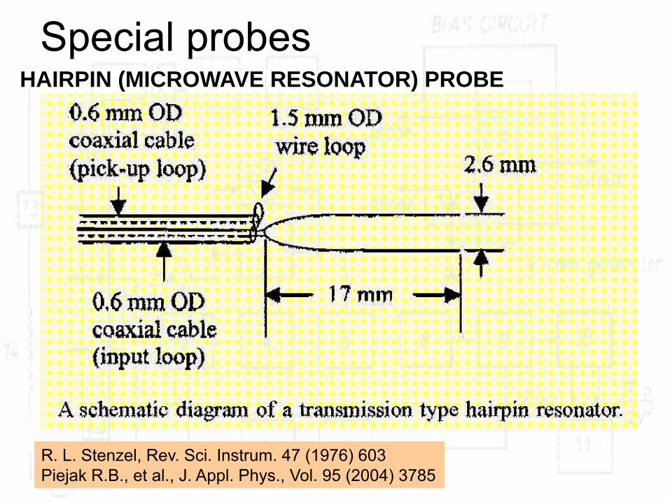
Special probesHAIRPIN (MICROWAVE RESONATOR) PROBE
R. L. Stenzel, Rev. Sci. Instrum. 47 (1976) 603Piejak R.B., et al., J. Appl. Phys., Vol. 95 (2004) 3785
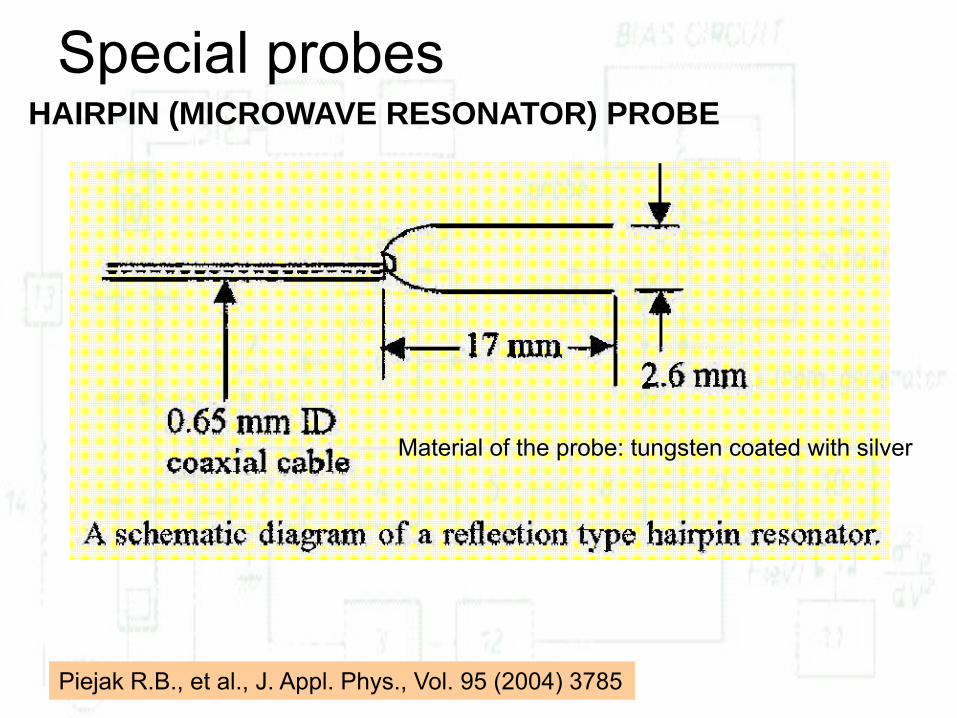
Special probesHAIRPIN (MICROWAVE RESONATOR) PROBE
Piejak R.B., et al., J. Appl. Phys., Vol. 95 (2004) 3785
Material of the probe: tungsten coated with silver
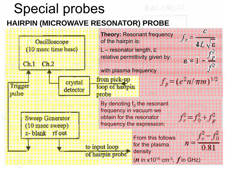
Special probesHAIRPIN (MICROWAVE RESONATOR) PROBE
Theory: Resonant frequency of the hairpin is:L – resonator length, εrelative permittivity given by:
with plasma frequency
By denoting f0 the resonant frequency in vacuum we obtain for the resonator frequency the expression:
From this followsfor the plasma density (n in x1010 cm-3, f in GHz)
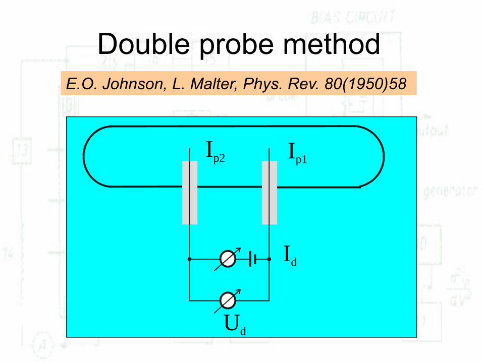
Double probe methodE.O. Johnson, L. Malter, Phys. Rev. 80(1950)58
Ip2 Ip1
Id
Ud
Double probe method
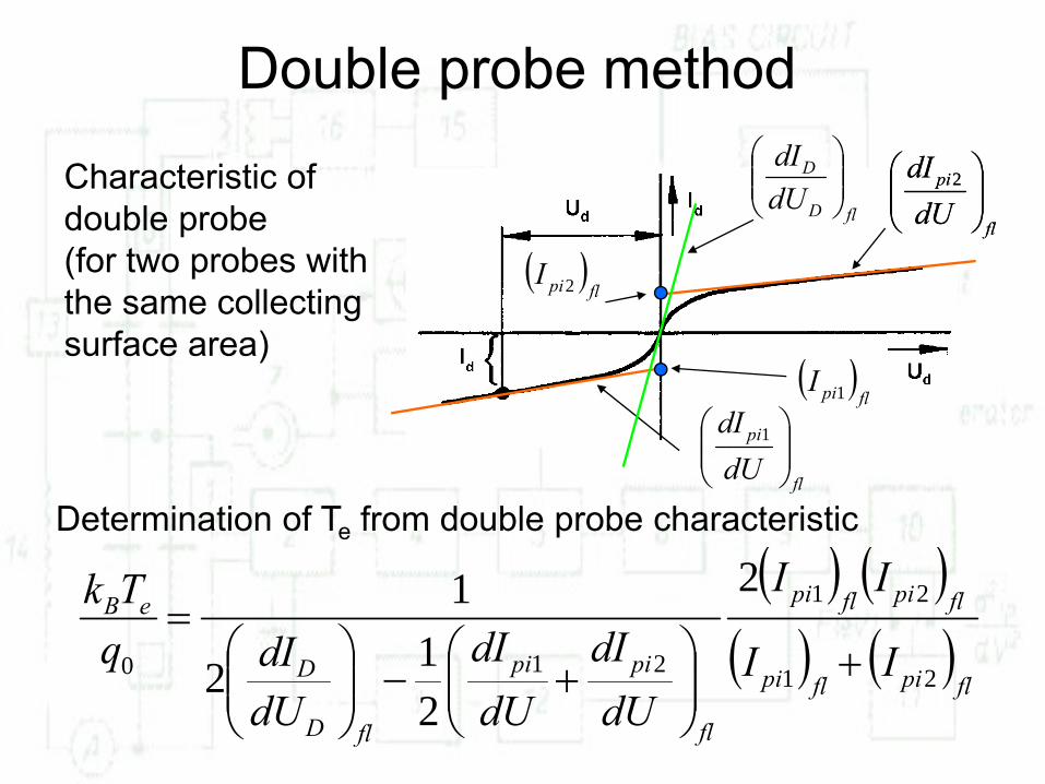
Characteristic of double probe (for two probes with the same collecting surface area)
Determination of Te from double probe characteristic
( ) ( )( ) ( )
flpiflpi
flpiflpi
fl
pipi
flD
D
eB
II
II
dUdI
dUdI
dUdIq
Tk
21
21
210
2
212
1
+⎟⎟⎠
⎞⎜⎜⎝
⎛+−⎟⎟
⎠
⎞⎜⎜⎝
⎛=
( )flpiI 1
( )flpiI 2
fl
pi
dUdI
⎟⎟⎠
⎞⎜⎜⎝
⎛ 1
fl
pi
dUdI
⎟⎟⎠
⎞⎜⎜⎝
⎛ 2
fl
pi
dUdI
⎟⎟⎠
⎞⎜⎜⎝
⎛ 2
flD
D
dUdI
⎟⎟⎠
⎞⎜⎜⎝
⎛
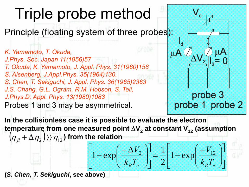
In the collisionless case it is possible to evaluate the electron temperature from one measured point ΔV2 at constant V12 (assumption
) from the relation
(S. Chen, T. Sekiguchi, see above)
Triple probe methodPrinciple (floating system of three probes):
K. Yamamoto, T. Okuda, J.Phys. Soc. Japan 11(1956)57T. Okuda, K. Yamamoto, J. Appl. Phys. 31(1960)158S. Aisenberg, J.Appl.Phys. 35(1964)130.S. Chen, T. Sekiguchi, J. Appl. Phys. 36(1965)2363J.S. Chang, G.L. Ogram, R.M. Hobson, S. Teii, J.Phys.D: Appl. Phys. 13(1980)1083Probes 1 and 3 may be asymmetrical.
( ) 122 ηηη ⟩⟩Δ+fl
⎥⎦
⎤⎢⎣
⎡⎟⎟⎠
⎞⎜⎜⎝
⎛ −−=⎥
⎦
⎤⎢⎣
⎡⎟⎟⎠
⎞⎜⎜⎝
⎛ Δ−−
eBeB TkV
TkV 122 exp1
21exp1
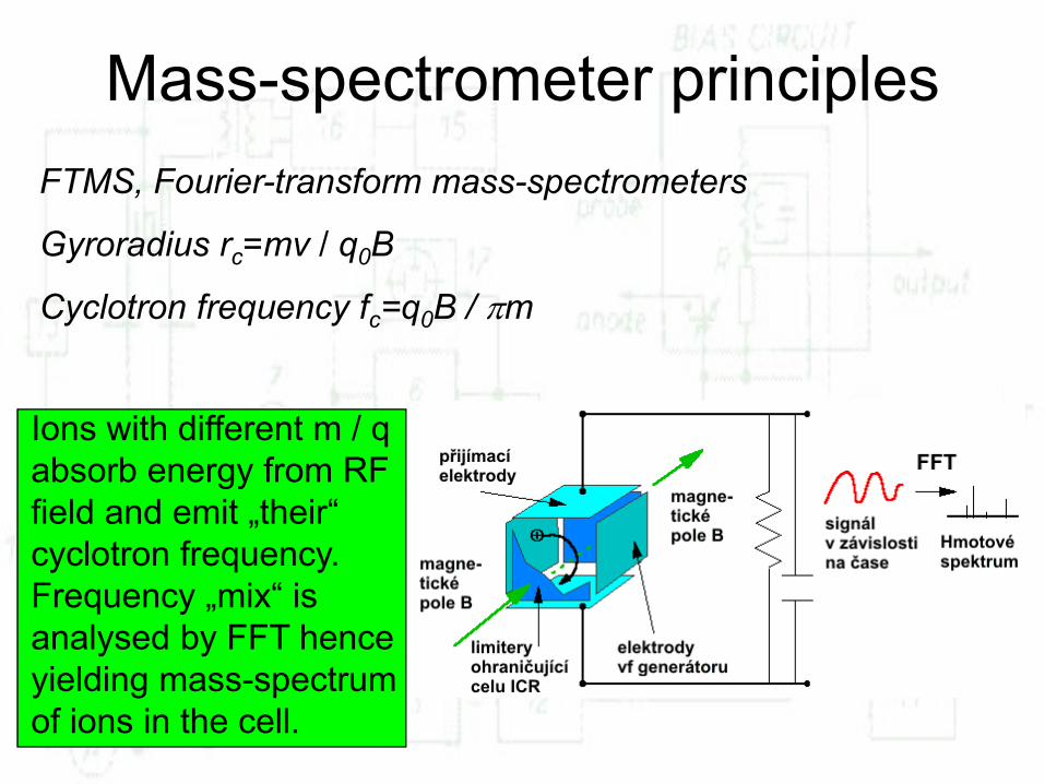
Ions with different m / q absorb energy from RF field and emit „their“ cyclotron frequency. Frequency „mix“ is analysed by FFT hence yielding mass-spectrum of ions in the cell.
Mass-spectrometer principles FTMS, Fourier-transform mass-spectrometers
Gyroradius rc=mv / q0B
Cyclotron frequency fc=q0B / πm
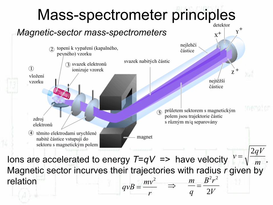
Mass-spectrometer principlesMagnetic-sector mass-spectrometers
Ions are accelerated to energy T=qV => have velocity .Magnetic sector incurves their trajectories with radius r given by relation
mqVv 2
=
rmvqvB
2
= VrB
qm
2
22
=⇒

Mass-spectrometer principlesTOFMS, time-of-flight mass-spectrometersIons are accelerated to energy T=qV => have velocity . They pass the same route L, mass-indicator is time t.
Since t = L / v, hence and .
Removal of thermal velocity spread – reflectron.
mqVv 2
=
VqmLt
21
= 2
22LVt
qm
=

Mass-spectrometer principlesQuadrupole mass-spectrometer
Mass spectrum is typically measured by varying amplitudes U (dc component) and V (ac component) whilekeeping constant the ratio U/Vat constant frequency. Mass resolution – stability diagram: A~U/m, Q~V/m. Quadrupole transparency decreases with increasing resolution power (adjustable by varying the ratio U/V).
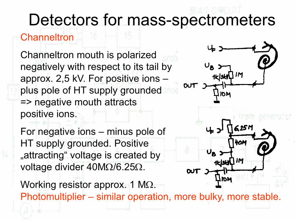
Channeltron
Channeltron mouth is polarized negatively with respect to its tail by approx. 2,5 kV. For positive ions –plus pole of HT supply grounded => negative mouth attracts positive ions.
For negative ions – minus pole of HT supply grounded. Positive „attracting“ voltage is created by voltage divider 40MΩ/6.25Ω.
Working resistor approx. 1 MΩ.
Detectors for mass-spectrometers
Photomultiplier – similar operation, more bulky, more stable.
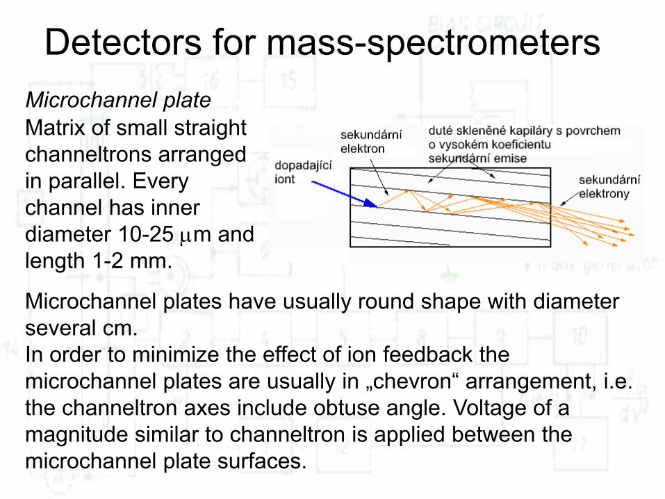
Detectors for mass-spectrometersMicrochannel plateMatrix of small straight channeltrons arranged in parallel. Every channel has inner diameter 10-25 μm and length 1-2 mm.
Microchannel plates have usually round shape with diameter several cm. In order to minimize the effect of ion feedback the microchannel plates are usually in „chevron“ arrangement, i.e. the channeltron axes include obtuse angle. Voltage of a magnitude similar to channeltron is applied between the microchannel plate surfaces.
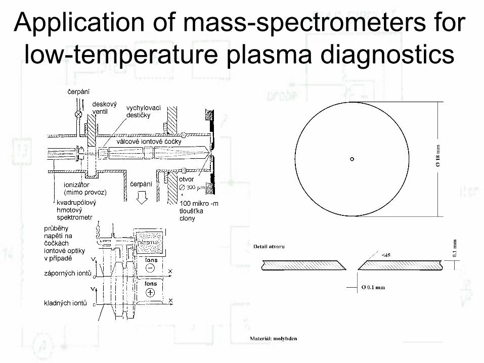
Application of mass-spectrometers for low-temperature plasma diagnostics

Application of mass-spectrometers for low-temperature plasma diagnostics
FALP apparatus (flowing afterglow Langmuir probe)Study of gas phase ion-molecule reactions
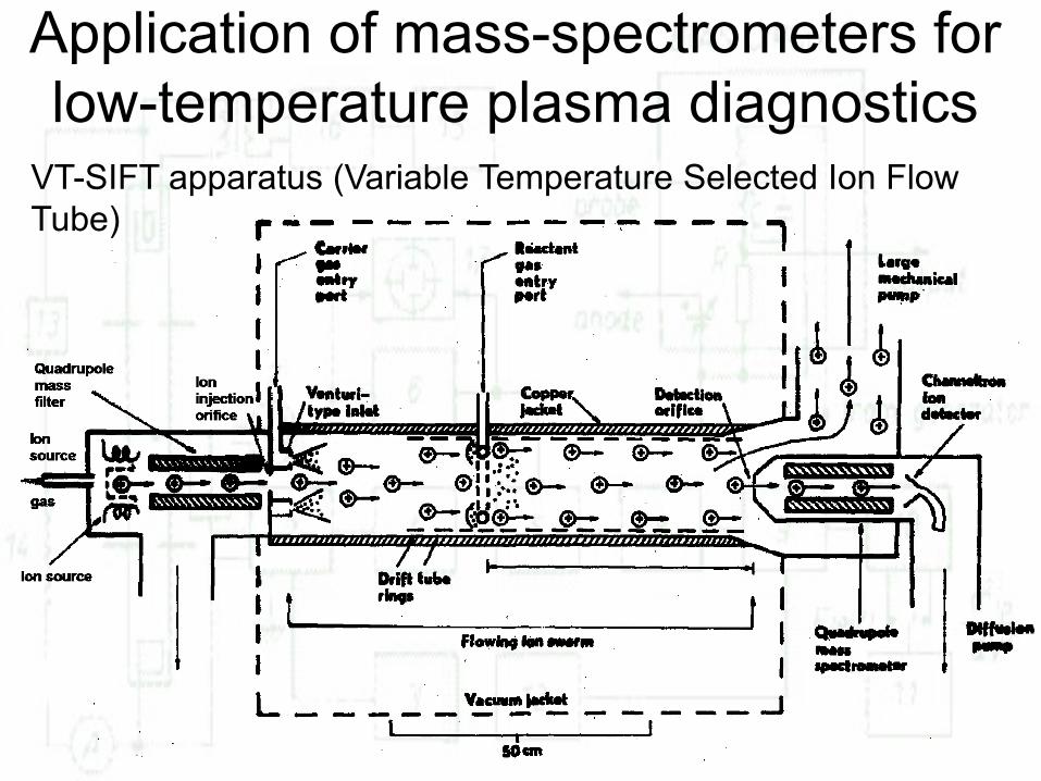
Application of mass-spectrometers for low-temperature plasma diagnostics
VT-SIFT apparatus (Variable Temperature Selected Ion Flow Tube)
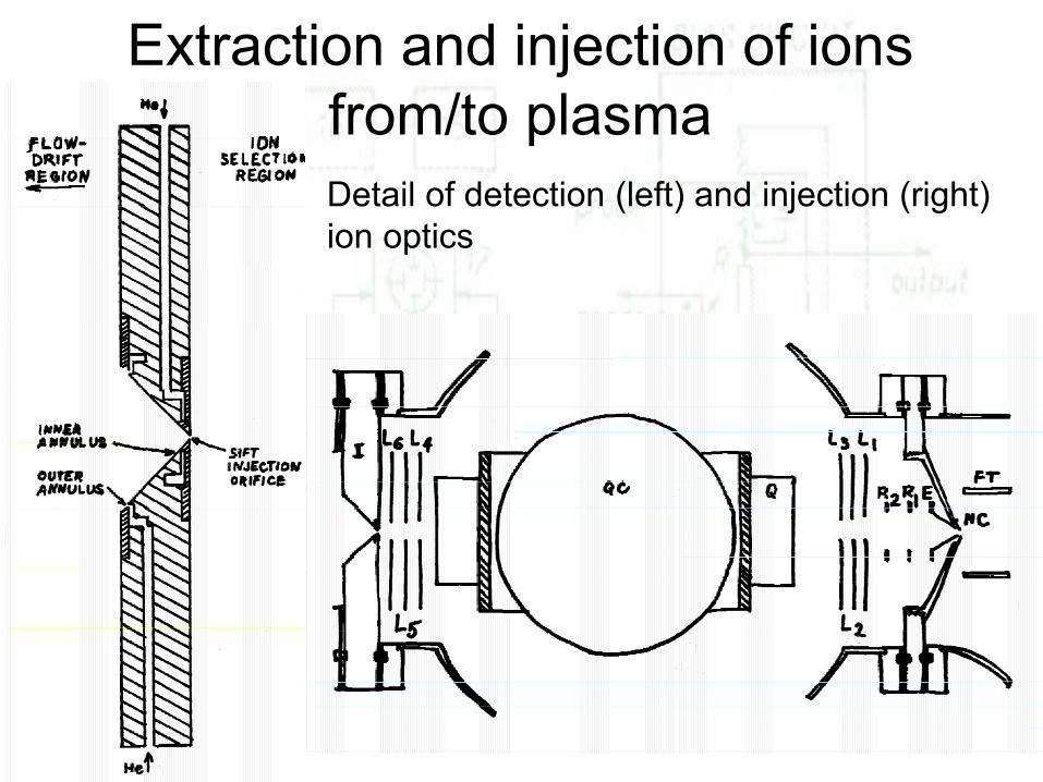
Extraction and injection of ions from/to plasmaDetail of detection (left) and injection (right) ion optics
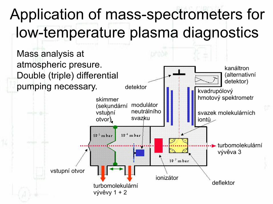
Application of mass-spectrometers for low-temperature plasma diagnosticsMass analysis at atmospheric presure. Double (triple) differential pumping necessary.
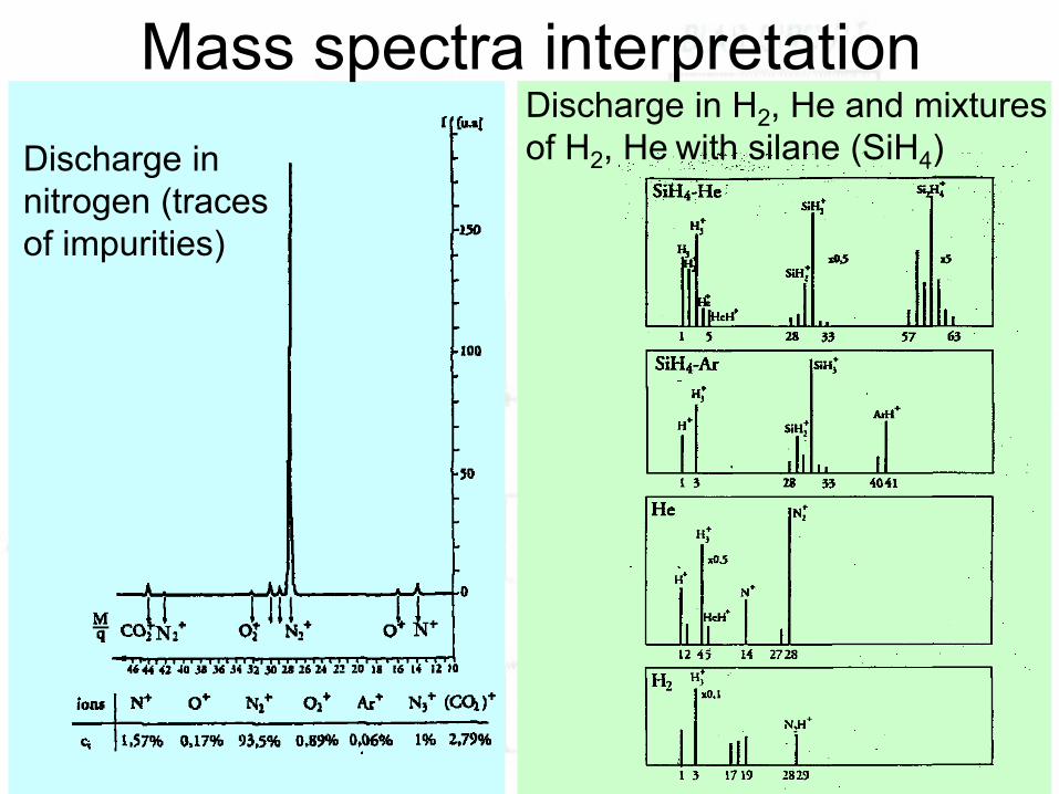
Mass spectra interpretationDischarge in nitrogen (traces of impurities)
Discharge in H2, He and mixtures of H2, He with silane (SiH4)
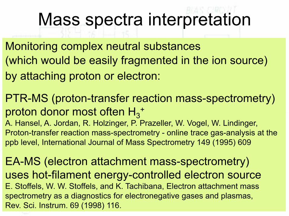
Mass spectra interpretationMonitoring complex neutral substances (which would be easily fragmented in the ion source) by attaching proton or electron:
PTR-MS (proton-transfer reaction mass-spectrometry)proton donor most often H3
+
A. Hansel, A. Jordan, R. Holzinger, P. Prazeller, W. Vogel, W. Lindinger, Proton-transfer reaction mass-spectrometry - online trace gas-analysis at the ppb level, International Journal of Mass Spectrometry 149 (1995) 609
EA-MS (electron attachment mass-spectrometry)uses hot-filament energy-controlled electron source E. Stoffels, W. W. Stoffels, and K. Tachibana, Electron attachment mass spectrometry as a diagnostics for electronegative gases and plasmas, Rev. Sci. Instrum. 69 (1998) 116.
Conclusion
• At the study of ion-molecule chemical reactions and at optimization of technological processes in low-temperature plasma the mass-spectrometer appears to be indispensable equipment.
• It is advantageous to combine the probe and the mass-spectrometer diagnostics together with other types of diagnostics, e.g. optical emission/absorption spectroscopy, microwave diagnostics, LIF, etc.

Thank you for your attention