Lam MasterTechWisk
55
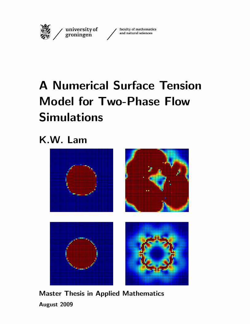
A Numerical Surface Tension Model for Two-Phase Flow Simulations K.W. Lam Master Thesis in Applied Mathematics August 2009
-
Upload
vinay-gupta -
Category
Documents
-
view
235 -
download
0
Transcript of Lam MasterTechWisk
A Numerical Surface Tension
Model for Two-Phase Flow
Simulations
K.W. Lam
Master Thesis in Applied Mathematics
August 2009

A Numerical Surface Tension Modelfor Two-Phase Flow Simulations
Summary
In two-phase flow simulations (for example air and water) the description of the fluid interfaceis important. For these simulations we have used a surface tension model. From literature weknow that the approximation of the surface curvature is important, for badly approximatedsurface curvatures will lead to spurious (unphysical) velocities.To track the surface interface we use a Volume of Fluid (VoF) method. Some researchers(Brackbill et al, Williams et al) say that this method will not work properly, so they modifiedit.By looking at the structure of our model, we thought that VoF would also work unmodified.We have tested our methods on a stationary bubble case, because then spurious currentsare best seen. The goal is to reduce these spurious currents, because they should not occur.During the talk we will compare results of our methods with results of the method that isbeing used in ComFlo.
Master Thesis in Applied MathematicsAuthor: K.W. LamSupervisor(s): A.E.P. Veldman and R. LuppesDate: August 2009
Institute of Mathematics and Computing ScienceP.O. Box 4079700 AK GroningenThe Netherlands

I would like to dedicate this thesis to my parents:To my mother, Cheung Pik Lin, who always is there for us.And to the memories of my father, Lam Tung Sing.
Contents
1 Introduction 1
2 The model 3
3 Literature review 53.1 A continuum method for modeling surface tension . . . . . . . . . . . . . . . 53.2 Accuracy and convergence of continuum surface tension models . . . . . . . . 63.3 A novel technique for including surface tension in PLIC-VOF methods . . . . 83.4 A front-tracking algorithm for accurate representation of surface tension . . . 103.5 Method used at RuG (program: ComFlo) . . . . . . . . . . . . . . . . . . . . 113.6 Height functions for applying contact angles to 3D VOF simulations . . . . . 123.7 Summary of methods . . . . . . . . . . . . . . . . . . . . . . . . . . . . . . . . 12
4 Discretization 154.1 The delta function δΓ = |∇C| . . . . . . . . . . . . . . . . . . . . . . . . . . . 154.2 Discretization of κ in 5 cells . . . . . . . . . . . . . . . . . . . . . . . . . . . . 154.3 Discretization of κ in > 5 cells . . . . . . . . . . . . . . . . . . . . . . . . . . 16
4.3.1 9 cells discretization . . . . . . . . . . . . . . . . . . . . . . . . . . . . 164.3.2 25 cells discretization based on Shirani et al. . . . . . . . . . . . . . . 18
4.4 3D discretizations . . . . . . . . . . . . . . . . . . . . . . . . . . . . . . . . . . 204.4.1 Discretization of κ in 27 cells (3D) . . . . . . . . . . . . . . . . . . . . 204.4.2 3D discretization based on Shirani et al. (125 cells) . . . . . . . . . . . 23
4.5 Free-surface displacement . . . . . . . . . . . . . . . . . . . . . . . . . . . . . 27
5 Results 315.1 Simulation done with the delta function 4C(1− C) . . . . . . . . . . . . . . . 315.2 5 cells vs. 9 cells discretization . . . . . . . . . . . . . . . . . . . . . . . . . . 335.3 Comparison with the height function method . . . . . . . . . . . . . . . . . . 35
5.3.1 The height function method vs. 9 cells discretization method . . . . . 355.3.2 The height function method vs. method based on Shirani’s unit normal 39
5.4 Results of 3D methods . . . . . . . . . . . . . . . . . . . . . . . . . . . . . . . 43
6 Conclusion 47
iii

iv CONTENTS
Chapter 1
Introduction
Two-phase flow problems, for example of a liquid and a gas, separated by a moving, deform-ing interface, are of interest in many research fields. Ranging from environmental sciencesto nuclear industries (power plants). It is desirable for researchers to be able to predict thebehaviour. To get more knowledge of such flows, they simulate these flows.In two-phase flow simulations, approximating the surface tension force term accurately isimportant, for not approximating this term properly will lead to spurious (non-physical) ve-locities. These spurious velocities are caused by the way the surface tension force is discretizedand the way the surface curvature κ is approximated [11]. Researchers all over the world aretrying to reduce these spurious velocities. Especially the curvature part is the subject ofstudy by many.To locate and track the surface interface the Volume of Fluid method (VoF) is widely used,because of its abilty to conserve mass, even when the topology changes. (As in joining orbreaking up of the fluids.)
Since the curvature κ = ∇ · ∇C
|∇C|, one might think that it can be approximated well by a
finite difference discretization method (FDM), but VoF turns out to be too abrupt for a finitedifference discretization. We can see that the values of the volume fractions function1 in thecells are changing abruptly. To be able to use a FDM, Brackbill et al. [1] are creating adifferent volume fraction function by mollifying (smoothing) the abrupt one. The alternativevolume fraction function is smooth enough, and Brackbill et al. are applying FDM to themollified volume fraction function to approximate κ. This method to approximate κ is usedby many researchers. Alternatively at the Groningen University the height function methodis used to approximate κ [8].Looking at the Navier-Stokes equations we wondered if it is really necessary to mollify first,and then use a FDM, since the pressure gradient shows the exact same abruptness. In thisproject we have looked at several finite difference discretizations, and we have compared thesediscretizations with the height function method. The discretizations will be given in chapter4. What we do looks like smoothing, since we use more and more cells, but the main differencewith Brackbill et al. [1] is that we do not change the volume fraction function, we use theoriginal abrupt one.First we will start with a literature review, where some other methods for approximating κwill pass by. Then we will give the discretizations of the methods that we have tried, and
1There will be an explanation in the next chapter what volume fractions are.
1

2 CHAPTER 1. INTRODUCTION
we will compare the results of these methods with the height function method. To test thesemethods, we have made use of a stationary bubble test-case, for it is easy to determine thespurious currents. More about the stationary bubble we can see in chapter 5. At the endsome conclusions will be given.
Chapter 2
The model
A two-phase flow is modelled with the Navier-Stokes equation
ρ
(∂u∂t
+ (u · ∇)u)
= −∇p +∇ · (µS) + F (2.1)
where ρ is the density (which is assumed to be piecewise constant in this thesis, therefore∇ · u = 0), µ the viscosity and S the rate of strain tensor
Sij =12
(∂uj
∂xi+
∂ui
∂xj
)and F = σκnδΓ+(∇σ)δΓ is the surface tension force, with σ the surface tension coefficient andδΓ a delta function concentrated on the surface interface Γ. The surface tension coefficient σis assumed to be constant, therefore the second term (∇σ)δΓ is neglected. So
F = σκnδΓ, (2.2)
where δΓ is a delta function. For δΓ there are many options.To model a two-phase flow problem we need to track the interface. For this the Volume ofFluid (VoF) method is used. A short explanation about this method will be given now.
Volume of Fluid method
In a VoF-method for a two-phase system a color function c, defined as
c(x) =
1 if x lies in fluid 1,
0 < c(x) < 1 if x lies in interface,0 if x lies in fluid 2
is used. The volume fraction function C is defined as
Ci =
∫Ωi
c(x)dΩi
|Ωi|, (2.3)
where Ωi is the corresponding cell. In 2D simulations |Ωi| is the area of the cell Ωi, in 3Dsimulations |Ωi| is the volume of Ωi.It then follows that a cell filled with fluid 1 has value C = 1, and a cell filled with fluid 2 has
3
4 CHAPTER 2. THE MODEL
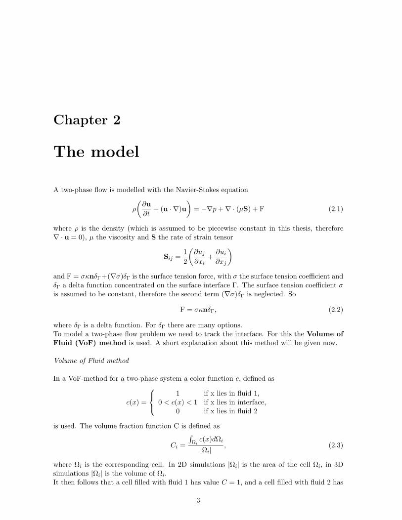
Figure 2.1: left: picture of the interface, right: corresponding volume fraction function
value C = 0. So when 0 < C < 1 (fluid 1 and fluid 2 mixed) holds for a given cell, this is aninterface cell. (See figure 2.1 for an example.)In this study we have done simulations with two discrete formulations of the delta functionsδΓ. We have also looked at how the curvature of the surface is determined numerically. Forthe curvature κ we use the following formulation
κ = ∇ · n with n =∇C
|∇C|(2.4)
where C is the volume fraction function, and n is the unit normal to the surface interface Γ.First a few methods of reseachers around the world are summarized in the next chapter, thenthe method that is being used at RuG will be explained.
Chapter 3
Literature review
As we have seen in the introduction, one of the reasons for the existence of spurious currentsis the bad approximations of interface curvature. Therefore to reduce spurious currents, re-searchers around the world have tried to improve the approximations of the curvature of theinterface. During a literature study we have studied several methods. Some of these methodsare summarized in this chapter.
3.1 A continuum method for modeling surface tension
J. U. Brackbill, D. B. Kothe and C. Zemach
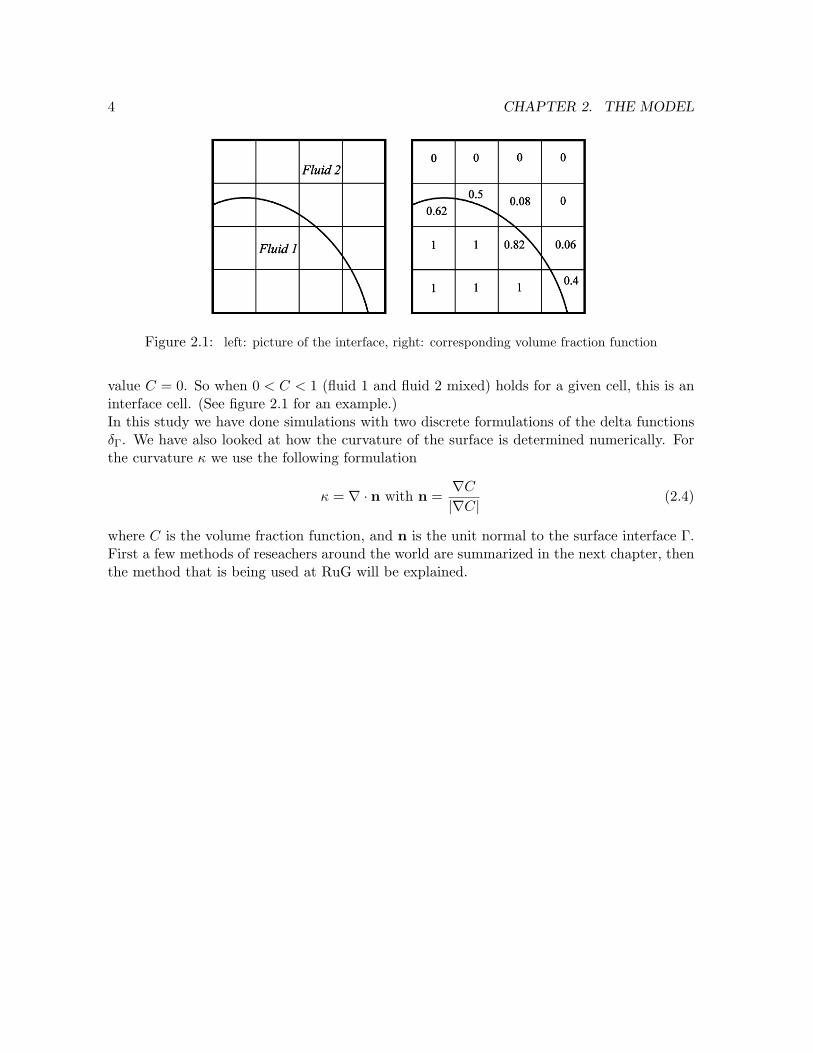
Figure 3.1: A surface interface with the corresponding volume fraction function.
In figure 3.1 we can see an example of a volume fraction function. We can see that it changesabruptly across the interface. Since we need the first and second derivative of the volumefraction function C to determine an approximation to n and κ respectively, this abruptnessof C might cause a problem.Brackbill et al. proposed a solution to this problem by first convolving C with a smooth
5
6 CHAPTER 3. LITERATURE REVIEW
kernel K to construct a smoothed or mollified function C.
C(x) = K ∗ C(x) =∫
Ωk
C(x′)K (x′ − x)dx′ (3.1)
Now n and κ follows from n =∇C
|∇C|and κ = −∇ · n
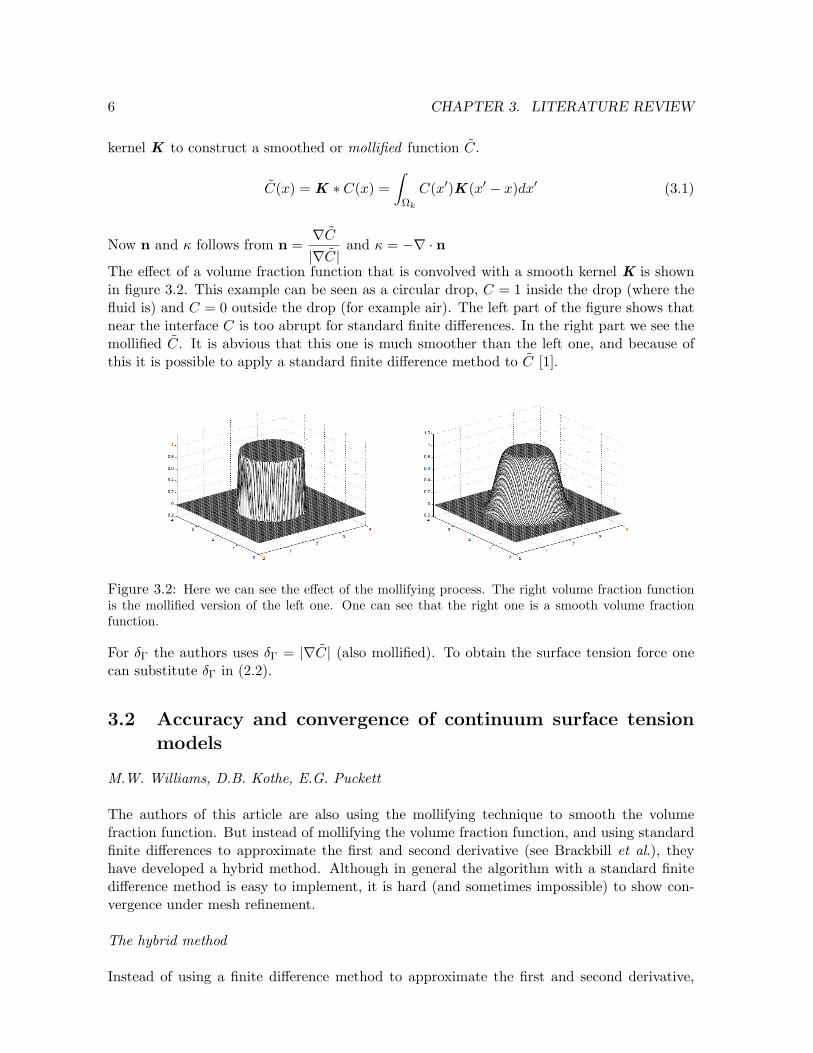
The effect of a volume fraction function that is convolved with a smooth kernel K is shownin figure 3.2. This example can be seen as a circular drop, C = 1 inside the drop (where thefluid is) and C = 0 outside the drop (for example air). The left part of the figure shows thatnear the interface C is too abrupt for standard finite differences. In the right part we see themollified C. It is abvious that this one is much smoother than the left one, and because ofthis it is possible to apply a standard finite difference method to C [1].
Figure 3.2: Here we can see the effect of the mollifying process. The right volume fraction functionis the mollified version of the left one. One can see that the right one is a smooth volume fractionfunction.
For δΓ the authors uses δΓ = |∇C| (also mollified). To obtain the surface tension force onecan substitute δΓ in (2.2).
3.2 Accuracy and convergence of continuum surface tensionmodels
M.W. Williams, D.B. Kothe, E.G. Puckett
The authors of this article are also using the mollifying technique to smooth the volumefraction function. But instead of mollifying the volume fraction function, and using standardfinite differences to approximate the first and second derivative (see Brackbill et al.), theyhave developed a hybrid method. Although in general the algorithm with a standard finitedifference method is easy to implement, it is hard (and sometimes impossible) to show con-vergence under mesh refinement.
The hybrid method
Instead of using a finite difference method to approximate the first and second derivative,
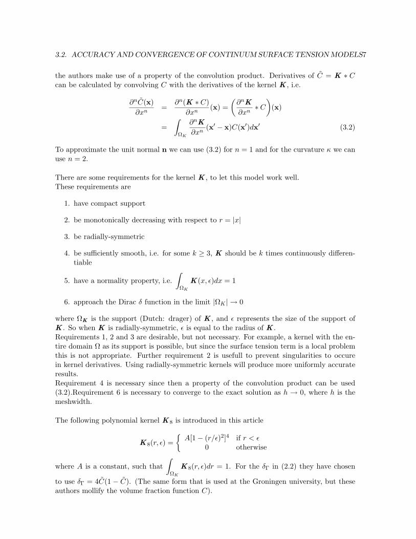
3.2. ACCURACY AND CONVERGENCE OF CONTINUUM SURFACE TENSION MODELS7
the authors make use of a property of the convolution product. Derivatives of C = K ∗ Ccan be calculated by convolving C with the derivatives of the kernel K , i.e.
∂nC(x)∂xn
=∂n(K ∗ C)
∂xn(x) =
(∂nK
∂xn∗ C
)(x)
=∫
ΩK
∂nK
∂xn(x′ − x)C(x′)dx′ (3.2)
To approximate the unit normal n we can use (3.2) for n = 1 and for the curvature κ we canuse n = 2.
There are some requirements for the kernel K , to let this model work well.These requirements are
1. have compact support
2. be monotonically decreasing with respect to r = |x|
3. be radially-symmetric
4. be sufficiently smooth, i.e. for some k ≥ 3, K should be k times continuously differen-tiable
5. have a normality property, i.e.∫
ΩK
K (x, ε)dx = 1
6. approach the Dirac δ function in the limit |ΩK | → 0
where ΩK is the support (Dutch: drager) of K , and ε represents the size of the support ofK . So when K is radially-symmetric, ε is equal to the radius of K .Requirements 1, 2 and 3 are desirable, but not necessary. For example, a kernel with the en-tire domain Ω as its support is possible, but since the surface tension term is a local problemthis is not appropriate. Further requirement 2 is usefull to prevent singularities to occurein kernel derivatives. Using radially-symmetric kernels will produce more uniformly accurateresults.Requirement 4 is necessary since then a property of the convolution product can be used(3.2).Requirement 6 is necessary to converge to the exact solution as h → 0, where h is themeshwidth.
The following polynomial kernel K 8 is introduced in this article
K 8(r, ε) =
A[1− (r/ε)2]4 if r < ε0 otherwise
where A is a constant, such that∫
ΩK
K 8(r, ε)dr = 1. For the δΓ in (2.2) they have chosen
to use δΓ = 4C(1 − C). (The same form that is used at the Groningen university, but theseauthors mollify the volume fraction function C).
8 CHAPTER 3. LITERATURE REVIEW
3.3 A novel technique for including surface tension in PLIC-VOF methods
Markus Meier, George Yadigaroglu, Brian L. Smith
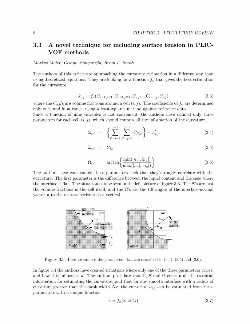
The authors of this article are approaching the curvature estimation in a different way thanusing discretized equations. They are looking for a function fκ that gives the best estimationfor the curvature.
ki,j = fκ(Ci±1,j±1, Ci±1,j∓1, Ci,j±1, Ci±1,j , Ci,j) (3.3)
where the Ca,b’s are volume fractions around a cell (i, j). The coefficients of fκ are determinedonly once and in advance, using a least-squares method against reference data.Since a function of nine variables is not convenient, the authors have defined only threeparameters for each cell (i, j), which should contain all the information of the curvature.
Σi,j = i+1∑
i′=i−1
j+1∑j′=j−1
Ci′,j′
−A′
i,j (3.4)
Ξi,j = Ci,j (3.5)
Ωi,j = arctan
min(|nx|, |ny|)max(|nx|, |ny|)
(3.6)
The authors have constructed these parameters such that they strongly correlate with thecurvature. The first parameter is the difference between the liquid content and the case wherethe interface is flat. The situation can be seen in the left picture of figure 3.3. The Ξ’s are justthe volume fractions in the cell itself, and the Ω’s are the tilt angles of the interface-normalvector n to the nearest horizontal or vertical.
Figure 3.3: Here we can see the parameters that are described in (3.4), (3.5) and (3.6).
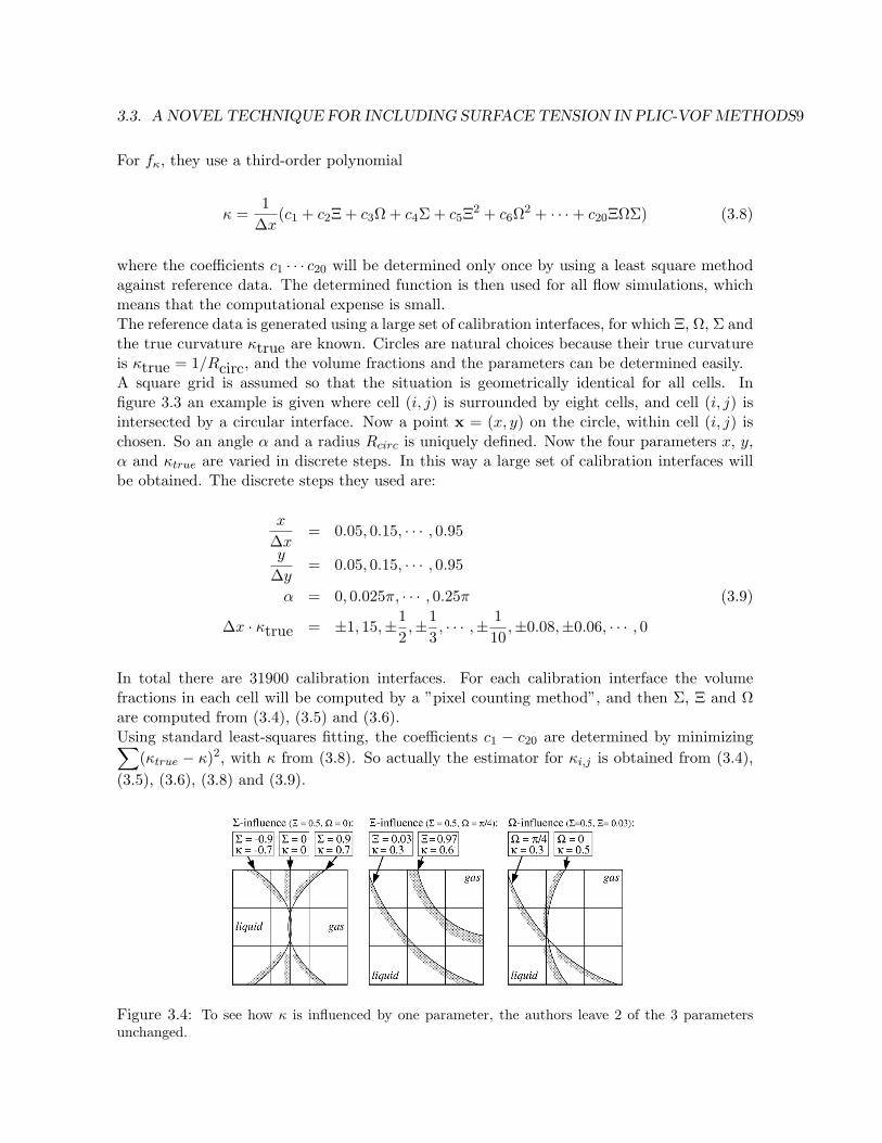
In figure 3.4 the authors have created situations where only one of the three parameters varies,and how this influences κ. The authors postulate that Σ, Ξ and Ω contain all the essentialinformation for estimating the curvature, and that for any smooth interface with a radius ofcurvature greater than the mesh-width ∆x, the curvature κi,j can be estimated from theseparameters with a unique function
κ = fκ(Σ,Ξ,Ω) (3.7)
3.3. A NOVEL TECHNIQUE FOR INCLUDING SURFACE TENSION IN PLIC-VOF METHODS9
For fκ, they use a third-order polynomial
κ =1
∆x(c1 + c2Ξ + c3Ω + c4Σ + c5Ξ2 + c6Ω2 + · · ·+ c20ΞΩΣ) (3.8)
where the coefficients c1 · · · c20 will be determined only once by using a least square methodagainst reference data. The determined function is then used for all flow simulations, whichmeans that the computational expense is small.The reference data is generated using a large set of calibration interfaces, for which Ξ, Ω, Σ andthe true curvature κtrue are known. Circles are natural choices because their true curvatureis κtrue = 1/Rcirc, and the volume fractions and the parameters can be determined easily.A square grid is assumed so that the situation is geometrically identical for all cells. Infigure 3.3 an example is given where cell (i, j) is surrounded by eight cells, and cell (i, j) isintersected by a circular interface. Now a point x = (x, y) on the circle, within cell (i, j) ischosen. So an angle α and a radius Rcirc is uniquely defined. Now the four parameters x, y,α and κtrue are varied in discrete steps. In this way a large set of calibration interfaces willbe obtained. The discrete steps they used are:
x
∆x= 0.05, 0.15, · · · , 0.95
y
∆y= 0.05, 0.15, · · · , 0.95
α = 0, 0.025π, · · · , 0.25π (3.9)
∆x · κtrue = ±1, 15,±12,±1
3, · · · ,± 1
10,±0.08,±0.06, · · · , 0
In total there are 31900 calibration interfaces. For each calibration interface the volumefractions in each cell will be computed by a ”pixel counting method”, and then Σ, Ξ and Ωare computed from (3.4), (3.5) and (3.6).Using standard least-squares fitting, the coefficients c1 − c20 are determined by minimizing∑
(κtrue − κ)2, with κ from (3.8). So actually the estimator for κi,j is obtained from (3.4),(3.5), (3.6), (3.8) and (3.9).
Figure 3.4: To see how κ is influenced by one parameter, the authors leave 2 of the 3 parametersunchanged.
10 CHAPTER 3. LITERATURE REVIEW
3.4 A front-tracking algorithm for accurate representation ofsurface tension
Stephane Popinet and Stephane Zaleski
Another different approach for attacking the term with the curvature is proposed by theseauthors. They are using the conservative form of (2.1)
∂ρu∂t
+∇ · (ρu⊗ u) = −∇p +∇ · (2µD) + σκδΓn (3.10)
The authors are using a momentum-conserving formulation of the Navier-Stokes equation.The pressure, volume fraction and velocity components are discretized on a uniform grid.Now the integral of the momentum equation is written as
∂
∂t
∫Ω
ρudx = L(u, χ)−∮
∂ΩpdΓ
where
L(u, χ) = −∮
∂Ωρu⊗ u · dΓ +
∮∂Ω
2µD · dΓ +∫
ΩσκδΓndx +
∫Ω
ρgdx. (3.11)
Here Ω is the control volume and ∂Ω is the boundary of the control volume. The article
concentrates on the term∫
ΩσκδΓndx.
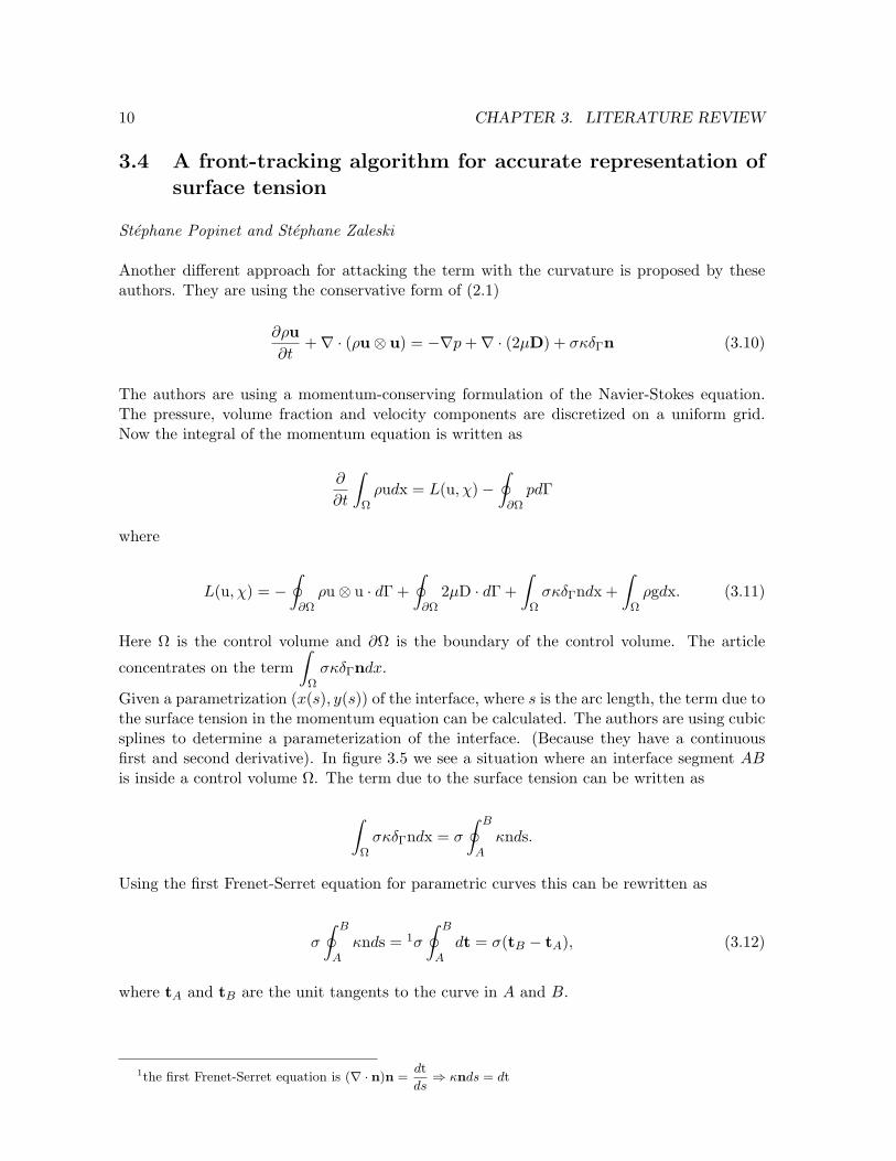
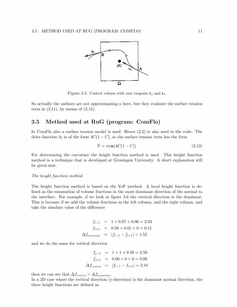
Given a parametrization (x(s), y(s)) of the interface, where s is the arc length, the term due tothe surface tension in the momentum equation can be calculated. The authors are using cubicsplines to determine a parameterization of the interface. (Because they have a continuousfirst and second derivative). In figure 3.5 we see a situation where an interface segment ABis inside a control volume Ω. The term due to the surface tension can be written as
∫Ω
σκδΓndx = σ
∮ B
Aκnds.
Using the first Frenet-Serret equation for parametric curves this can be rewritten as
σ
∮ B
Aκnds = 1σ
∮ B
Adt = σ(tB − tA), (3.12)
where tA and tB are the unit tangents to the curve in A and B.
1the first Frenet-Serret equation is (∇ · n)n =dt
ds⇒ κnds = dt
3.5. METHOD USED AT RUG (PROGRAM: COMFLO) 11
Figure 3.5: Control volume with unit tangents ta and tb.
So actually the authors are not approximating κ here, but they evaluate the surface tensionterm in (3.11), by means of (3.12).
3.5 Method used at RuG (program: ComFlo)
In ComFlo also a surface tension model is used. Hence (2.2) is also used in the code. Thedelta function δΓ is of the form 4C(1− C), so the surface tension term has the form
F = σκn(4C(1− C)) (3.13)
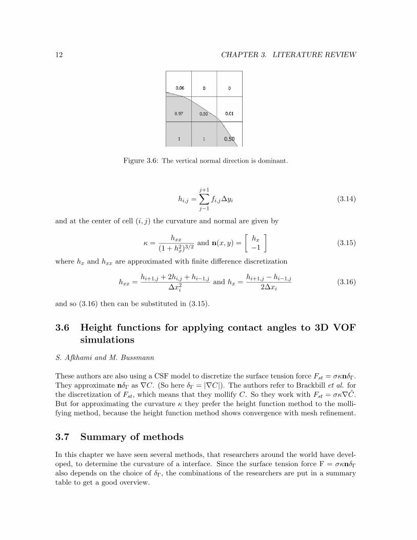
For determining the curvature the height function method is used. This height functionmethod is a technique that is developed at Groningen University. A short explanation willbe given now.
The height function method
The height function method is based on the VoF method. A local height function is de-fined as the summation of volume fractions in the most dominant direction of the normal tothe interface. For example, if we look at figure 3.6 the vertical direction is the dominant.This is because if we add the volume fractions in the left column, and the right column, andtake the absolute value of the difference
fi−1 = 1 + 0.97 + 0.06 = 2.03fi+1 = 0.50 + 0.01 + 0 = 0.51
∆fhorizontal = |fi−1 − fi+1| = 1.52
and we do the same for vertical direction
fj−1 = 1 + 1 + 0.50 = 2.50fj+1 = 0.06 + 0 + 0 = 0.06
∆fvertical = |fi−1 − fi+1| = 2.44
then we can see that ∆fvertical > ∆fhorizontal.In a 2D case where the vertical direction (y-direction) is the dominant normal direction, thethree height functions are defined as
12 CHAPTER 3. LITERATURE REVIEW
Figure 3.6: The vertical normal direction is dominant.
hi,j =j+1∑j−1
fi,j∆yi (3.14)
and at the center of cell (i, j) the curvature and normal are given by
κ =hxx
(1 + h2x)3/2
and n(x, y) =[
hx
−1
](3.15)
where hx and hxx are approximated with finite difference discretization
hxx =hi+1,j + 2hi,j + hi−1,j
∆x2i
and hx =hi+1,j − hi−1,j
2∆xi(3.16)
and so (3.16) then can be substituted in (3.15).
3.6 Height functions for applying contact angles to 3D VOFsimulations
S. Afkhami and M. Bussmann
These authors are also using a CSF model to discretize the surface tension force Fst = σκnδΓ.They approximate nδΓ as ∇C. (So here δΓ = |∇C|). The authors refer to Brackbill et al. forthe discretization of Fst, which means that they mollify C. So they work with Fst = σκ∇C.But for approximating the curvature κ they prefer the height function method to the molli-fying method, because the height function method shows convergence with mesh refinement.
3.7 Summary of methods
In this chapter we have seen several methods, that researchers around the world have devel-oped, to determine the curvature of a interface. Since the surface tension force F = σκnδΓ
also depends on the choice of δΓ, the combinations of the researchers are put in a summarytable to get a good overview.
3.7. SUMMARY OF METHODS 13
authors curvature κ δ functionBrackbill et al. [1] mollify with a smooth ker-
nel|∇C|
Williams et al. [7] hybrid method 4C(1− C)
Meier et al. [2] using least square methodto determine function
δΓn =∇ρ(x)
(ρl − ρg)2ρ(x)
(ρl + ρg)
Popinet & Zaleski [4] using momentum preserv-ing formulation of NS(unit tangents)
1st Frenet-Serret eqn. usedto evaluate the σ term
M. ten Caat et al. [8] height function 4C(1− C)
Afkhami & Bussmann [9] height function |∇C|
To approximate n =∇C
|∇C|and κ = ∇ · n, where C is the volume fraction function, it is
straightforward to first try a finite difference method, but it turns out that finite differencemethods cannot handle the abruptness of the volume fraction function. To attack this prob-lem, Brackbill et al. [1] mollify the volume fraction function with a smooth kernel K to obtaina new function that is smooth enough for finite difference methods (see figure 3.2).To approximate κ Williams et al. are also using the mollifying technique, but the main differ-ence with Brackbill et al. [1] is that they make use of a property of the convolution product.Instead of using a finite difference method to approximate the first and second derivative ofthe mollified volume fraction function, they convolve the volume fraction function with thefirst and second derivative of the smooth kernel K . This hybrid method will give betterresults.Meier et al. [2] approach the curvature approximation in a different way. With a least squareestimation they determine a function κ in terms of the surrounding volume fractions. (9 in2D and 27 in 3D). Once this function is known they can fill in the volume fractions to get thelocal κ.Popinet and Zaleski [4] are making use of a momentum preserving formulation of the Navier-Stokes equation. With the first Frenet-Serret equation they are able to rewrite the surfacetension term in terms of unit tangents to the surface in certain points (see figure 3.5).For approximation of κ Veldman et al. have developed the height function method. Unlikethe finite difference methods the height function does converge with mesh-refinement. Thismethod is used by many researchers, e.g. Afkhami and Bussmann [9] are using the heightfunction to approximate κ.
During the project we thought that it would be interesting to try a discretization of n =∇C
|∇C|,
with unmollified C, anyway. The idea is that finite differences should be able to handle theabruptness of C, since the pressure gradient possesses the same abruptness. For δΓ, |∇C|is chosen, which we will also leave unmollified. Our main reason is that it would be inter-
14 CHAPTER 3. LITERATURE REVIEW
esting to be able to compare different choices of δΓ. But later we found out that choosingδΓ = 4C(1−C) is not appropriate. This can be shown by looking at the units. If we look at(2.1) we see that −∇p should have the same unit as F = σκnδΓ. Since
[p] =Nm2
⇒ [∇p] =Nm3
also [F] =Nm3
must hold for δΓ = 4C(1 − C). But now we have [σ] =Nm
, [κ] =1m
,n =
unitless and so is 4C(1 − C), so we have [F] =Nm2
. Hence we can see that there is missing
a factor1m
, when δΓ = 4C(1− C) is used.
On the other hand if we look at δΓ = |∇C|, we then have F = σκ∇C (see (4.1)). Since
[∇C] =1m
we are not missing the factor1m
. In chapter 4 we will see some results with bothdelta functions.First we will look at the discretizations, which can be found in the next chapter.
Chapter 4
Discretization
In this chapter the delta function δΓ = |∇C|, the unit normal n =∇C
|∇C|and the surface curvature κ =
∇ · n will be discretized. This will be done with a finite difference method, both over 5 and9 cells in 2D (and a 3D version of the 9 cells discretization over 27 cells). Also will we makeuse of the unit normal, that we have found in an article by Shirani et al. [6], to discretizeκ = ∇ · n in 2D (over 25 cells) and in 3D (over 125 cells).
4.1 The delta function δΓ = |∇C|First of all, we take a look at F = σκnδΓ. Since |∇C| is chosen as the delta function, we have
F = σκn|∇C|. Since n =∇C
|∇C|⇒ ∇C = n|∇C|. Therefore we get
F = σκ∇C (4.1)
The discretization of ∇C (in 2 dimensions) is straightforward
in i direction ∇Cx =C(i + 1, j)− C(i, j)
dx
in j direction ∇Cy =C(i, j + 1)− C(i, j)
dy
Now we will proceed with the discretizations of κ.
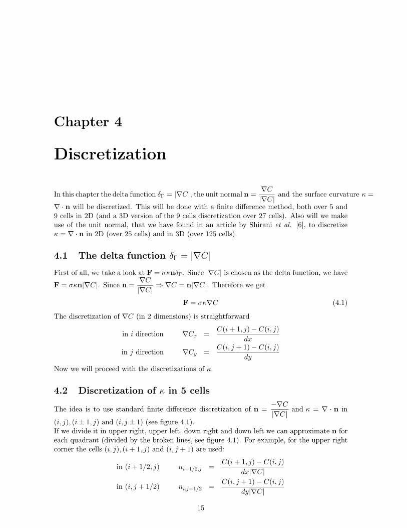
4.2 Discretization of κ in 5 cells
The idea is to use standard finite difference discretization of n =−∇C
|∇C|and κ = ∇ · n in
(i, j), (i± 1, j) and (i, j ± 1) (see figure 4.1).If we divide it in upper right, upper left, down right and down left we can approximate n foreach quadrant (divided by the broken lines, see figure 4.1). For example, for the upper rightcorner the cells (i, j), (i + 1, j) and (i, j + 1) are used:
in (i + 1/2, j) ni+1/2,j =C(i + 1, j)− C(i, j)
dx|∇C|
in (i, j + 1/2) ni,j+1/2 =C(i, j + 1)− C(i, j)
dy|∇C|
15
16 CHAPTER 4. DISCRETIZATION
where
∇C =(
C(i + 1, j)− C(i, j)dx
,C(i, j + 1)− C(i, j)
dy
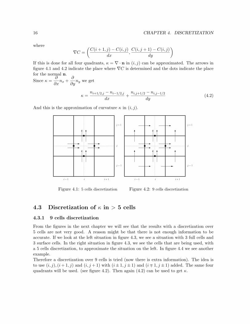
)If this is done for all four quadrants, κ = ∇ · n in (i, j) can be approximated. The arrows infigure 4.1 and 4.2 indicate the place where ∇C is determined and the dots indicate the placefor the normal n.Since κ =
∂
∂xnx +
∂
∂yny we get
κ =ni+1/2,j − ni−1/2,j
dx+
ni,j+1/2 − ni,j−1/2
dy(4.2)
And this is the approximation of curvature κ in (i, j).
i− 1 i i + 1
j − 1
j
j + 1
Figure 4.1: 5 cells discretization
i− 1 i i + 1
j − 1
j
j + 1
Figure 4.2: 9 cells discretization
4.3 Discretization of κ in > 5 cells
4.3.1 9 cells discretization
From the figures in the next chapter we will see that the results with a discretization over5 cells are not very good. A reason might be that there is not enough information to beaccurate. If we look at the left situation in figure 4.3, we see a situation with 3 full cells and3 surface cells. In the right situation in figure 4.3, we see the cells that are being used, witha 5 cells discretization, to approximate the situation on the left. In figure 4.4 we see anotherexample.Therefore a discretization over 9 cells is tried (now there is extra information). The idea isto use (i, j), (i + 1, j) and (i, j + 1) with (i± 1, j ± 1) and (i∓ 1, j ± 1) added. The same fourquadrants will be used. (see figure 4.2). Then again (4.2) can be used to get κ.
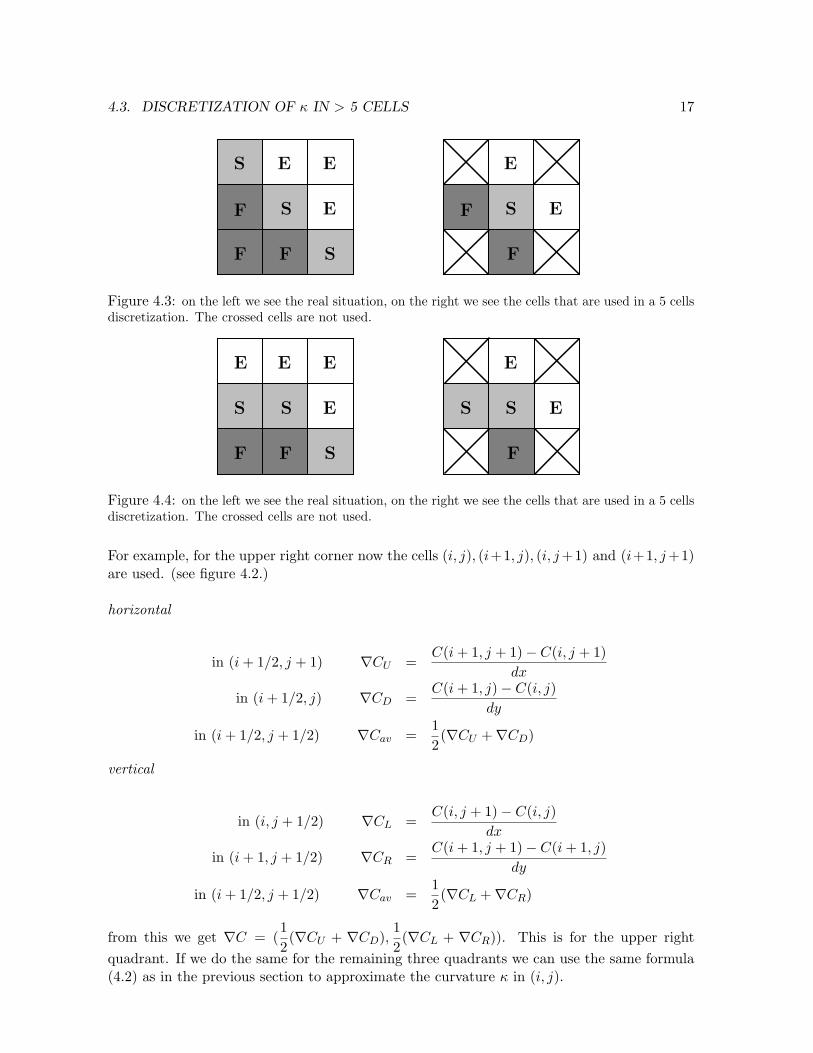
4.3. DISCRETIZATION OF κ IN > 5 CELLS 17
S
E
E
SFF
E
EF S
F
S E
F
Figure 4.3: on the left we see the real situation, on the right we see the cells that are used in a 5 cellsdiscretization. The crossed cells are not used.
S
E E
E
SF
E
ES
F
SS
F
E
Figure 4.4: on the left we see the real situation, on the right we see the cells that are used in a 5 cellsdiscretization. The crossed cells are not used.
For example, for the upper right corner now the cells (i, j), (i+1, j), (i, j +1) and (i+1, j +1)are used. (see figure 4.2.)
horizontal
in (i + 1/2, j + 1) ∇CU =C(i + 1, j + 1)− C(i, j + 1)
dx
in (i + 1/2, j) ∇CD =C(i + 1, j)− C(i, j)
dy
in (i + 1/2, j + 1/2) ∇Cav =12(∇CU +∇CD)
vertical
in (i, j + 1/2) ∇CL =C(i, j + 1)− C(i, j)
dx
in (i + 1, j + 1/2) ∇CR =C(i + 1, j + 1)− C(i + 1, j)
dy
in (i + 1/2, j + 1/2) ∇Cav =12(∇CL +∇CR)
from this we get ∇C = (12(∇CU + ∇CD),
12(∇CL + ∇CR)). This is for the upper right
quadrant. If we do the same for the remaining three quadrants we can use the same formula(4.2) as in the previous section to approximate the curvature κ in (i, j).
18 CHAPTER 4. DISCRETIZATION
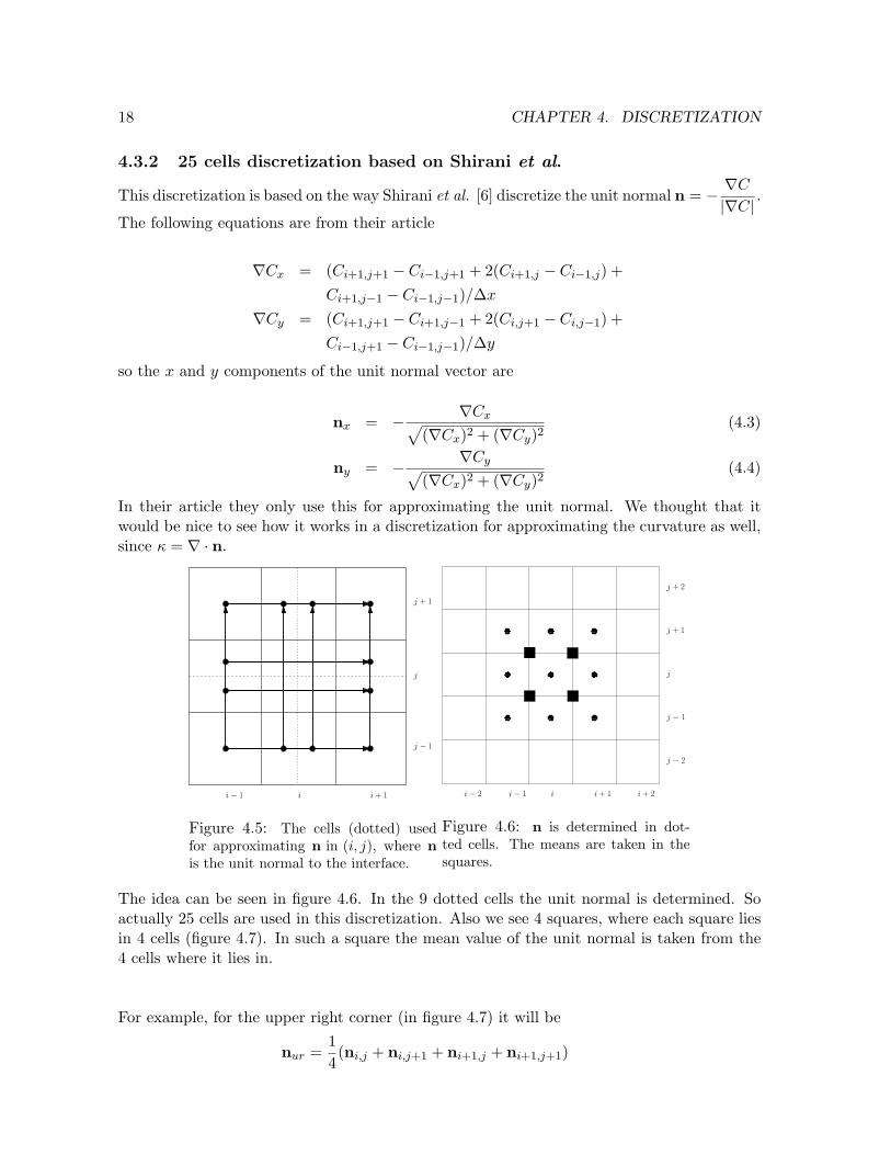
4.3.2 25 cells discretization based on Shirani et al.
This discretization is based on the way Shirani et al. [6] discretize the unit normal n = − ∇C
|∇C|.
The following equations are from their article
∇Cx = (Ci+1,j+1 − Ci−1,j+1 + 2(Ci+1,j − Ci−1,j) +Ci+1,j−1 − Ci−1,j−1)/∆x
∇Cy = (Ci+1,j+1 − Ci+1,j−1 + 2(Ci,j+1 − Ci,j−1) +Ci−1,j+1 − Ci−1,j−1)/∆y
so the x and y components of the unit normal vector are
nx = − ∇Cx√(∇Cx)2 + (∇Cy)2
(4.3)
ny = − ∇Cy√(∇Cx)2 + (∇Cy)2
(4.4)
In their article they only use this for approximating the unit normal. We thought that itwould be nice to see how it works in a discretization for approximating the curvature as well,since κ = ∇ · n.
i− 1 i i + 1
j − 1
j
j + 1
Figure 4.5: The cells (dotted) usedfor approximating n in (i, j), where nis the unit normal to the interface.
i i + 1
j + 2
j + 1
j
j − 1
j − 2
i− 2 i− 1 i + 2
Figure 4.6: n is determined in dot-ted cells. The means are taken in thesquares.
The idea can be seen in figure 4.6. In the 9 dotted cells the unit normal is determined. Soactually 25 cells are used in this discretization. Also we see 4 squares, where each square liesin 4 cells (figure 4.7). In such a square the mean value of the unit normal is taken from the4 cells where it lies in.
For example, for the upper right corner (in figure 4.7) it will be
nur =14(ni,j + ni,j+1 + ni+1,j + ni+1,j+1)
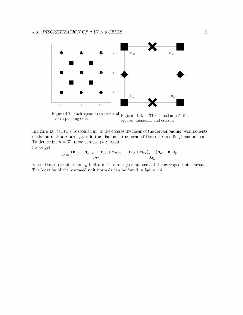
4.3. DISCRETIZATION OF κ IN > 5 CELLS 19
j + 1
j
j − 1
i− 1 i i + 1
Figure 4.7: Each square is the mean of4 corresponding dots.
j
i
nul
nll nlr
nur
Figure 4.8: The location of thesquares, diamonds and crosses.
In figure 4.8, cell (i, j) is zoomed in. In the crosses the mean of the corresponding j-componentsof the normals are taken, and in the diamonds the mean of the corresponding i-components.To determine κ = ∇ · n we can use (4.2) again.So we get
κ =(nur + nlr)x − (nul + nll)x
2dx+
(nul + nur)y − (nll + nlr)y
2dy
where the subscripts x and y indicate the x and y component of the averaged unit normals.The location of the averaged unit normals can be found in figure 4.8.
20 CHAPTER 4. DISCRETIZATION
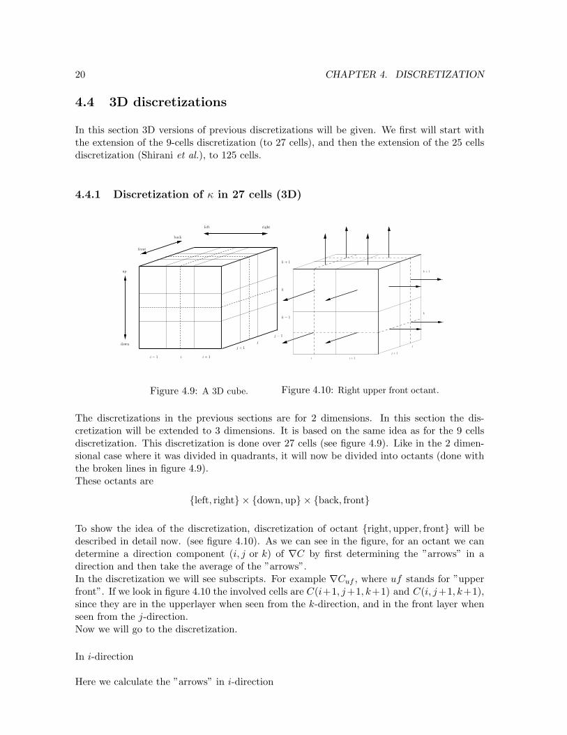
4.4 3D discretizations
In this section 3D versions of previous discretizations will be given. We first will start withthe extension of the 9-cells discretization (to 27 cells), and then the extension of the 25 cellsdiscretization (Shirani et al.), to 125 cells.
4.4.1 Discretization of κ in 27 cells (3D)
i + 1i− 1 i
k + 1
k
k − 1
j + 1
j − 1
j
left
back
front
right
down
up
Figure 4.9: A 3D cube.
i + 1
j + 1
j
k + 1
k
i
Figure 4.10: Right upper front octant.
The discretizations in the previous sections are for 2 dimensions. In this section the dis-cretization will be extended to 3 dimensions. It is based on the same idea as for the 9 cellsdiscretization. This discretization is done over 27 cells (see figure 4.9). Like in the 2 dimen-sional case where it was divided in quadrants, it will now be divided into octants (done withthe broken lines in figure 4.9).These octants are
left, right × down,up × back, front
To show the idea of the discretization, discretization of octant right,upper, front will bedescribed in detail now. (see figure 4.10). As we can see in the figure, for an octant we candetermine a direction component (i, j or k) of ∇C by first determining the ”arrows” in adirection and then take the average of the ”arrows”.In the discretization we will see subscripts. For example ∇Cuf , where uf stands for ”upperfront”. If we look in figure 4.10 the involved cells are C(i+1, j+1, k+1) and C(i, j+1, k+1),since they are in the upperlayer when seen from the k-direction, and in the front layer whenseen from the j-direction.Now we will go to the discretization.
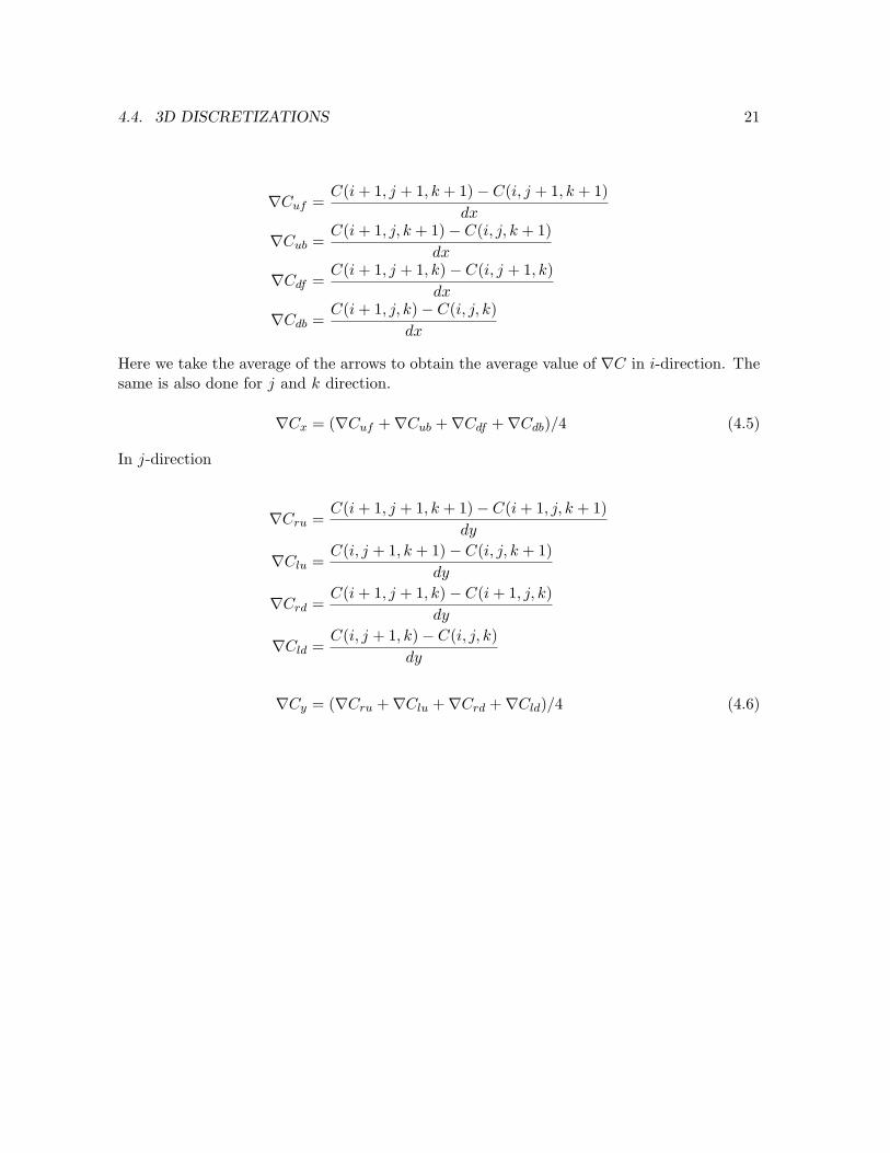
In i-direction
Here we calculate the ”arrows” in i-direction
4.4. 3D DISCRETIZATIONS 21
∇Cuf =C(i + 1, j + 1, k + 1)− C(i, j + 1, k + 1)
dx
∇Cub =C(i + 1, j, k + 1)− C(i, j, k + 1)
dx
∇Cdf =C(i + 1, j + 1, k)− C(i, j + 1, k)
dx
∇Cdb =C(i + 1, j, k)− C(i, j, k)
dx
Here we take the average of the arrows to obtain the average value of ∇C in i-direction. Thesame is also done for j and k direction.
∇Cx = (∇Cuf +∇Cub +∇Cdf +∇Cdb)/4 (4.5)
In j-direction
∇Cru =C(i + 1, j + 1, k + 1)− C(i + 1, j, k + 1)
dy
∇Clu =C(i, j + 1, k + 1)− C(i, j, k + 1)
dy
∇Crd =C(i + 1, j + 1, k)− C(i + 1, j, k)
dy
∇Cld =C(i, j + 1, k)− C(i, j, k)
dy
∇Cy = (∇Cru +∇Clu +∇Crd +∇Cld)/4 (4.6)
22 CHAPTER 4. DISCRETIZATION
In k-direction
∇Crf =C(i + 1, j + 1, k + 1)− C(i + 1, j + 1, k)
dz
∇Clf =C(i, j + 1, k + 1)− C(i, j + 1, k)
dz
∇Crb =C(i + 1, j, k + 1)− C(i + 1, j, k)
dz
∇Clb =C(i, j, k + 1)− C(i, j, k)
dz
∇Cz = (∇Crf +∇Clf +∇Crb +∇Clb)/4 (4.7)
So with (4.5),(4.6) and (4.7) we get
∇Cruf = (∇Cx,∇Cy,∇Cz) ⇒ |∇Cruf | =√
(∇Cx)2 + (∇Cy)2 + (∇Cz)2
And for the unit normal in octant right,upper, front we get
nruf =(
∇Cx
|∇Cruf |,∇Cy
|∇Cruf |,∇Cz
|∇Cruf |
)(4.8)
In the same way we can determine the direction of the normals for the other 7 octants. Forevery octant we then have normal component in i, j and k direction. If we look at the com-ponents in i-direction (see figure 4.11) we can determine the average of these components.(The big arrows in the figure).
nfnb
Figure 4.11: The 8 normal components in i-direction, where the big arrows are the average of 4corresponding small ones.
When this is also done for j and k direction we can use
κ =nf − nb
dx+
nr − nl
dy+
nu − nd
dz(4.9)
to obtain κ.
4.4. 3D DISCRETIZATIONS 23
4.4.2 3D discretization based on Shirani et al. (125 cells)
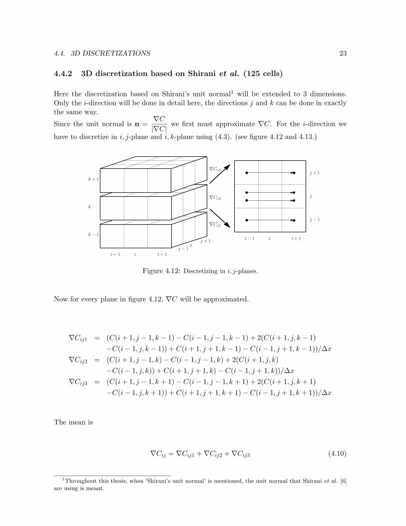
Here the discretization based on Shirani’s unit normal1 will be extended to 3 dimensions.Only the i-direction will be done in detail here, the directions j and k can be done in exactlythe same way.
Since the unit normal is n =∇C
|∇C|we first must approximate ∇C. For the i-direction we
have to discretize in i, j-plane and i, k-plane using (4.3). (see figure 4.12 and 4.13.)
i + 1ii− 1
k
k − 1i + 1ii− 1
j + 1
j
j − 1
j − 1j
j + 1
k + 1
∇Cij3
∇Cij2
∇Cij1
Figure 4.12: Discretizing in i, j-planes.
Now for every plane in figure 4.12, ∇C will be approximated.
∇Cij1 = (C(i + 1, j − 1, k − 1)− C(i− 1, j − 1, k − 1) + 2(C(i + 1, j, k − 1)−C(i− 1, j, k − 1)) + C(i + 1, j + 1, k − 1)− C(i− 1, j + 1, k − 1))/∆x
∇Cij2 = (C(i + 1, j − 1, k)− C(i− 1, j − 1, k) + 2(C(i + 1, j, k)−C(i− 1, j, k)) + C(i + 1, j + 1, k)− C(i− 1, j + 1, k))/∆x
∇Cij3 = (C(i + 1, j − 1, k + 1)− C(i− 1, j − 1, k + 1) + 2(C(i + 1, j, k + 1)−C(i− 1, j, k + 1)) + C(i + 1, j + 1, k + 1)− C(i− 1, j + 1, k + 1))/∆x
The mean is
∇Cij = ∇Cij1 +∇Cij2 +∇Cij3 (4.10)
1Throughout this thesis, when ’Shirani’s unit normal’ is mentioned, the unit normal that Shirani et al. [6]are using is meant.
24 CHAPTER 4. DISCRETIZATION
i− 1 i i + 1j − 1
j
j + 1
i + 1ii− 1
k + 1
k
k − 1
k + 1
k
k − 1
∇Cik3
∇Cik2
∇Cik1
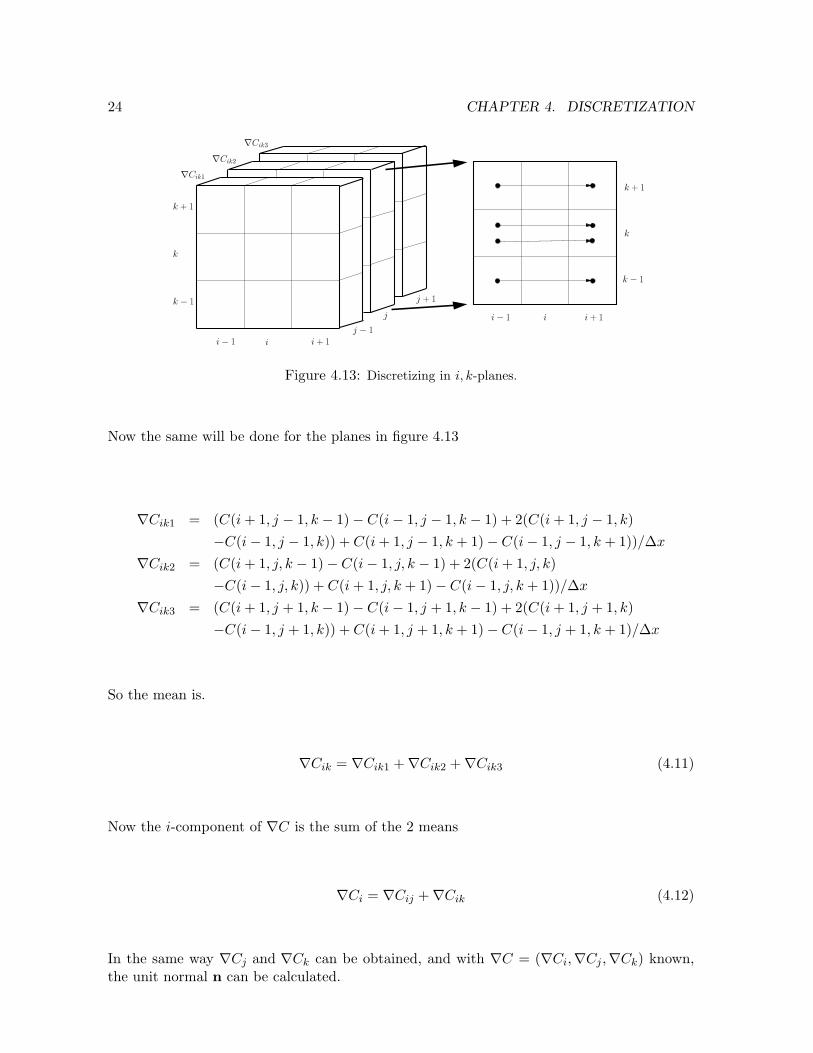
Figure 4.13: Discretizing in i, k-planes.
Now the same will be done for the planes in figure 4.13
∇Cik1 = (C(i + 1, j − 1, k − 1)− C(i− 1, j − 1, k − 1) + 2(C(i + 1, j − 1, k)−C(i− 1, j − 1, k)) + C(i + 1, j − 1, k + 1)− C(i− 1, j − 1, k + 1))/∆x
∇Cik2 = (C(i + 1, j, k − 1)− C(i− 1, j, k − 1) + 2(C(i + 1, j, k)−C(i− 1, j, k)) + C(i + 1, j, k + 1)− C(i− 1, j, k + 1))/∆x
∇Cik3 = (C(i + 1, j + 1, k − 1)− C(i− 1, j + 1, k − 1) + 2(C(i + 1, j + 1, k)−C(i− 1, j + 1, k)) + C(i + 1, j + 1, k + 1)− C(i− 1, j + 1, k + 1)/∆x
So the mean is.
∇Cik = ∇Cik1 +∇Cik2 +∇Cik3 (4.11)
Now the i-component of ∇C is the sum of the 2 means
∇Ci = ∇Cij +∇Cik (4.12)
In the same way ∇Cj and ∇Ck can be obtained, and with ∇C = (∇Ci,∇Cj ,∇Ck) known,the unit normal n can be calculated.
4.4. 3D DISCRETIZATIONS 25
i
k
k − 1
k + 1
k + 2
k − 2
j + 2j + 1
i− 2 i− 1 i + 1 i + 2
j − 2j − 1
j
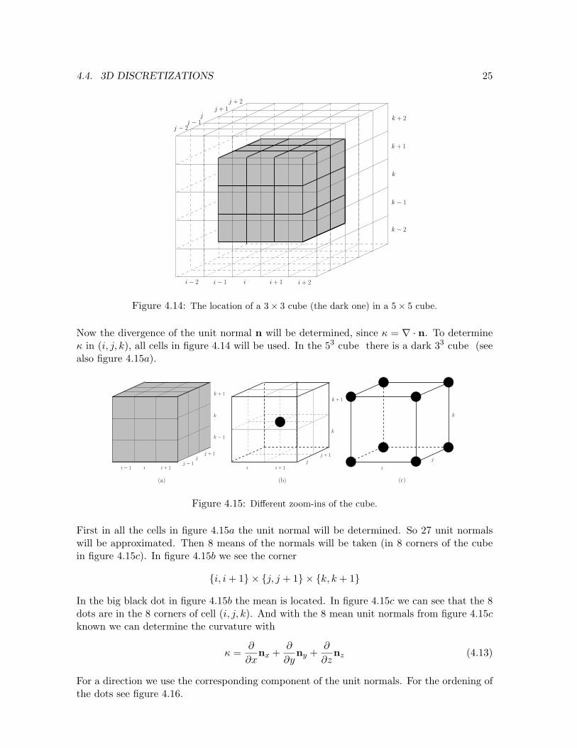
Figure 4.14: The location of a 3× 3 cube (the dark one) in a 5× 5 cube.
Now the divergence of the unit normal n will be determined, since κ = ∇ · n. To determineκ in (i, j, k), all cells in figure 4.14 will be used. In the 53 cube there is a dark 33 cube (seealso figure 4.15a).
i
j
k
i i + 1j
j + 1
k
k + 1
k
k + 1
k − 1
j + 1
j − 1ii− 1
j
(a) (c)(b)
i + 1
Figure 4.15: Different zoom-ins of the cube.
First in all the cells in figure 4.15a the unit normal will be determined. So 27 unit normalswill be approximated. Then 8 means of the normals will be taken (in 8 corners of the cubein figure 4.15c). In figure 4.15b we see the corner
i, i + 1 × j, j + 1 × k, k + 1
In the big black dot in figure 4.15b the mean is located. In figure 4.15c we can see that the 8dots are in the 8 corners of cell (i, j, k). And with the 8 mean unit normals from figure 4.15cknown we can determine the curvature with
κ =∂
∂xnx +
∂
∂yny +
∂
∂znz (4.13)
For a direction we use the corresponding component of the unit normals. For the ordening ofthe dots see figure 4.16.
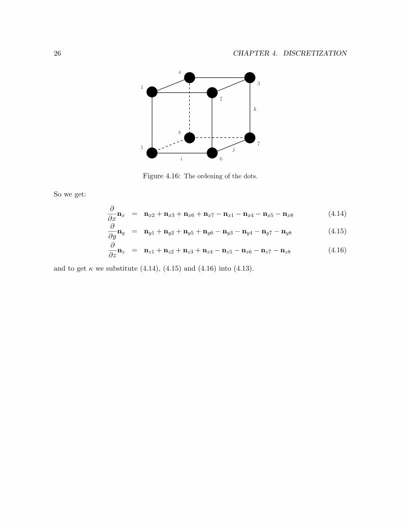
26 CHAPTER 4. DISCRETIZATION
i
j
k
1
4
2
3
5
6
7
8
Figure 4.16: The ordening of the dots.
So we get:
∂
∂xnx = nx2 + nx3 + nx6 + nx7 − nx1 − nx4 − nx5 − nx8 (4.14)
∂
∂yny = ny1 + ny2 + ny5 + ny6 − ny3 − ny4 − ny7 − ny8 (4.15)
∂
∂znz = nz1 + nz2 + nz3 + nz4 − nz5 − nz6 − nz7 − nz8 (4.16)
and to get κ we substitute (4.14), (4.15) and (4.16) into (4.13).
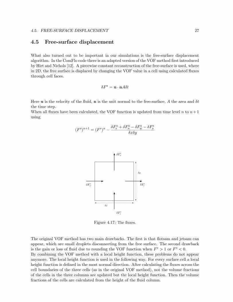
4.5. FREE-SURFACE DISPLACEMENT 27
4.5 Free-surface displacement
What also turned out to be important in our simulations is the free-surface displacementalgorithm. In the ComFlo code there is an adapted version of the VOF method first introducedby Hirt and Nichols [12]. A piecewise constant reconstruction of the free-surface is used, wherein 2D, the free surface is displaced by changing the VOF value in a cell using calculated fluxesthrough cell faces.
δF s = u · nAδt
Here u is the velocity of the fluid, n is the unit normal to the free-surface, A the area and δtthe time step.When all fluxes have been calculated, the VOF function is updated from time level n to n+1using
(F s)n+1 = (F s)n − δF se + δF s
n − δF sw − δF s
s
δxδy
δF sn
δF ss
δy
δx
δF sw δF s
e
Figure 4.17: The fluxes.
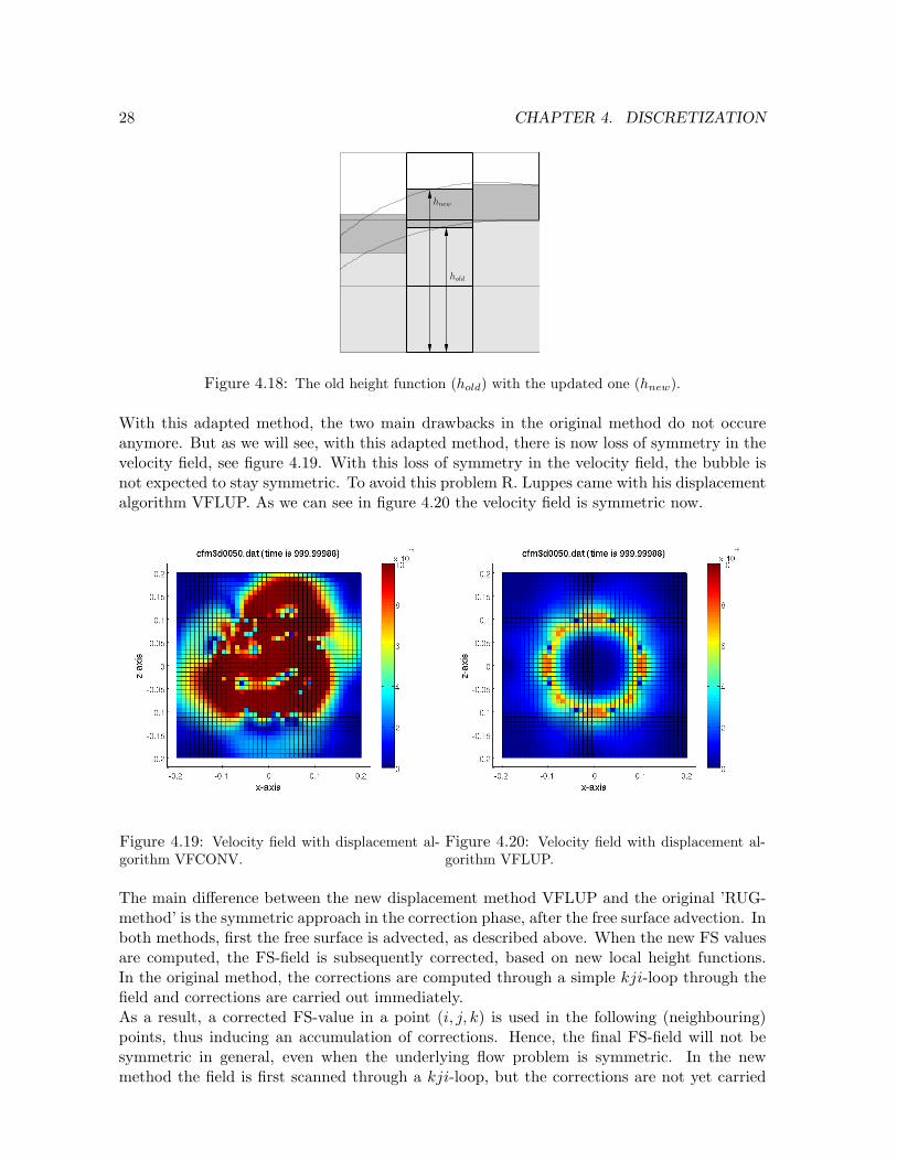
The original VOF method has two main drawbacks. The first is that flotsam and jetsam canappear, which are small droplets disconnecting from the free surface. The second drawbackis the gain or loss of fluid due to rounding the VOF function when F s > 1 or F s < 0.By combining the VOF method with a local height function, these problems do not appearanymore. The local height function is used in the following way. For every surface cell a localheight function is defined in the most normal direction. After calculating the fluxes across thecell boundaries of the three cells (as in the original VOF method), not the volume fractionsof the cells in the three columns are updated but the local height function. Then the volumefractions of the cells are calculated from the height of the fluid column.
28 CHAPTER 4. DISCRETIZATION
hnew
hold
Figure 4.18: The old height function (hold) with the updated one (hnew).
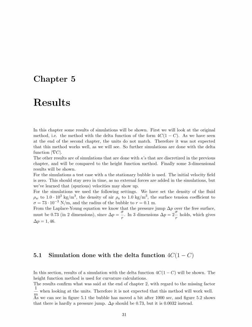
With this adapted method, the two main drawbacks in the original method do not occureanymore. But as we will see, with this adapted method, there is now loss of symmetry in thevelocity field, see figure 4.19. With this loss of symmetry in the velocity field, the bubble isnot expected to stay symmetric. To avoid this problem R. Luppes came with his displacementalgorithm VFLUP. As we can see in figure 4.20 the velocity field is symmetric now.
Figure 4.19: Velocity field with displacement al-gorithm VFCONV.
Figure 4.20: Velocity field with displacement al-gorithm VFLUP.
The main difference between the new displacement method VFLUP and the original ’RUG-method’ is the symmetric approach in the correction phase, after the free surface advection. Inboth methods, first the free surface is advected, as described above. When the new FS valuesare computed, the FS-field is subsequently corrected, based on new local height functions.In the original method, the corrections are computed through a simple kji-loop through thefield and corrections are carried out immediately.As a result, a corrected FS-value in a point (i, j, k) is used in the following (neighbouring)points, thus inducing an accumulation of corrections. Hence, the final FS-field will not besymmetric in general, even when the underlying flow problem is symmetric. In the newmethod the field is first scanned through a kji-loop, but the corrections are not yet carried

4.5. FREE-SURFACE DISPLACEMENT 29
out. The effect of possible corrections is monitored and stored and all possible correctionsare gathered. When the full field is scanned, the corrections are carried out, still based onthe height function approach. This results in a symmetric correction of the FS-field. Whenthe underlying flow problem is symmetric, the final FS-field will also be symmetric.

30 CHAPTER 4. DISCRETIZATION
Chapter 5
Results
In this chapter some results of simulations will be shown. First we will look at the originalmethod, i.e. the method with the delta function of the form 4C(1 − C). As we have seenat the end of the second chapter, the units do not match. Therefore it was not expectedthat this method works well, as we will see. So further simulations are done with the deltafunction |∇C|.The other results are of simulations that are done with κ’s that are discretized in the previouschapter, and will be compared to the height function method. Finally some 3-dimensionalresults will be shown.For the simulations a test case with a the stationary bubble is used. The initial velocity fieldis zero. This should stay zero in time, as no external forces are added in the simulations, butwe’ve learned that (spurious) velocities may show up.For the simulations we used the following settings. We have set the density of the fluidρw to 1.0 · 103 kg/m3, the density of air ρa to 1.0 kg/m3, the surface tension coefficient toσ = 73 · 10−3 N/m, and the radius of the bubble to r = 0.1 m.From the Laplace-Young equation we know that the pressure jump ∆p over the free surface,must be 0.73 (in 2 dimensions), since ∆p =
σ
r. In 3 dimensions ∆p = 2
σ
rholds, which gives
∆p = 1, 46.
5.1 Simulation done with the delta function 4C(1− C)
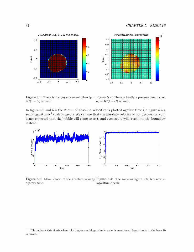
In this section, results of a simulation with the delta function 4C(1−C) will be shown. Theheight function method is used for curvature calculations.The results confirm what was said at the end of chapter 2, with regard to the missing factor1m
when looking at the units. Therefore it is not expected that this method will work well.As we can see in figure 5.1 the bubble has moved a bit after 1000 sec, and figure 5.2 showsthat there is hardly a pressure jump. ∆p should be 0.73, but it is 0.0032 instead.
31
32 CHAPTER 5. RESULTS
Figure 5.1: There is obvious movement when δΓ =4C(1− C) is used.
Figure 5.2: There is hardly a pressure jump whenδΓ = 4C(1− C) is used.
In figure 5.3 and 5.4 the 2norm of absolute velocities is plotted against time (in figure 5.4 asemi-logarithmic1 scale is used.) We can see that the absolute velocity is not decreasing, so itis not expected that the bubble will come to rest, and eventually will crash into the boundaryinstead.
Figure 5.3: Mean 2norm of the absolute velocityagainst time.
Figure 5.4: The same as figure 5.3, but now inlogarithmic scale.
1Throughout this thesis when ’plotting on semi-logarithmic scale’ is mentioned, logarithmic to the base 10is meant.
5.2. 5 CELLS VS. 9 CELLS DISCRETIZATION 33
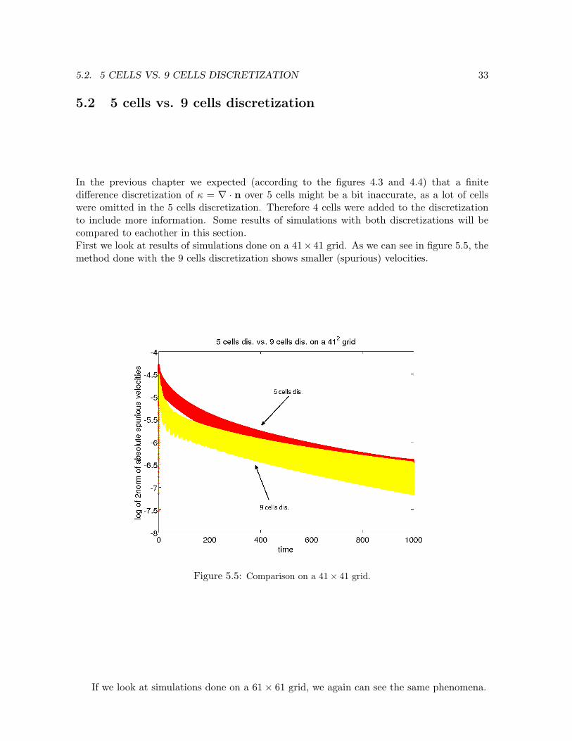
5.2 5 cells vs. 9 cells discretization
In the previous chapter we expected (according to the figures 4.3 and 4.4) that a finitedifference discretization of κ = ∇ · n over 5 cells might be a bit inaccurate, as a lot of cellswere omitted in the 5 cells discretization. Therefore 4 cells were added to the discretizationto include more information. Some results of simulations with both discretizations will becompared to eachother in this section.First we look at results of simulations done on a 41× 41 grid. As we can see in figure 5.5, themethod done with the 9 cells discretization shows smaller (spurious) velocities.
Figure 5.5: Comparison on a 41× 41 grid.
If we look at simulations done on a 61× 61 grid, we again can see the same phenomena.
34 CHAPTER 5. RESULTS
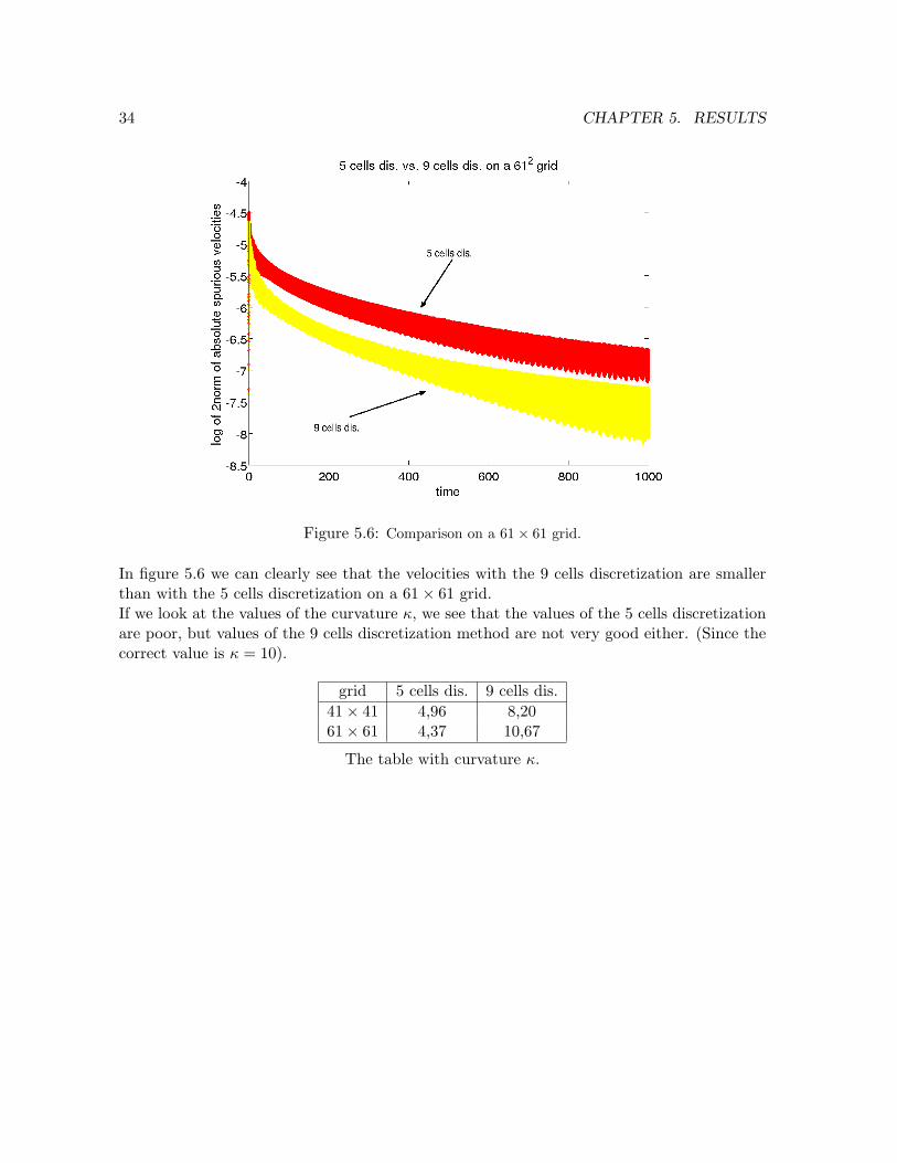
Figure 5.6: Comparison on a 61× 61 grid.
In figure 5.6 we can clearly see that the velocities with the 9 cells discretization are smallerthan with the 5 cells discretization on a 61× 61 grid.If we look at the values of the curvature κ, we see that the values of the 5 cells discretizationare poor, but values of the 9 cells discretization method are not very good either. (Since thecorrect value is κ = 10).
grid 5 cells dis. 9 cells dis.41× 41 4,96 8,2061× 61 4,37 10,67
The table with curvature κ.
5.3. COMPARISON WITH THE HEIGHT FUNCTION METHOD 35
5.3 Comparison with the height function method
In the previous section we have seen the accuracy of both the 5 cells discretization methodand the 9 cells discretization method. We have seen that both method are not good withregard to spurious velocities. Albeit the poor results we like to compare the best of these twomethods with the height function method. So in this section the height function method willbe compared with the 9 cells discretization of κ = ∇ · n. Further a comparison will be donewith the height function method and the method of the discretization of κ based on Shirani’sdiscretization of the unit normal [6].
5.3.1 The height function method vs. 9 cells discretization method
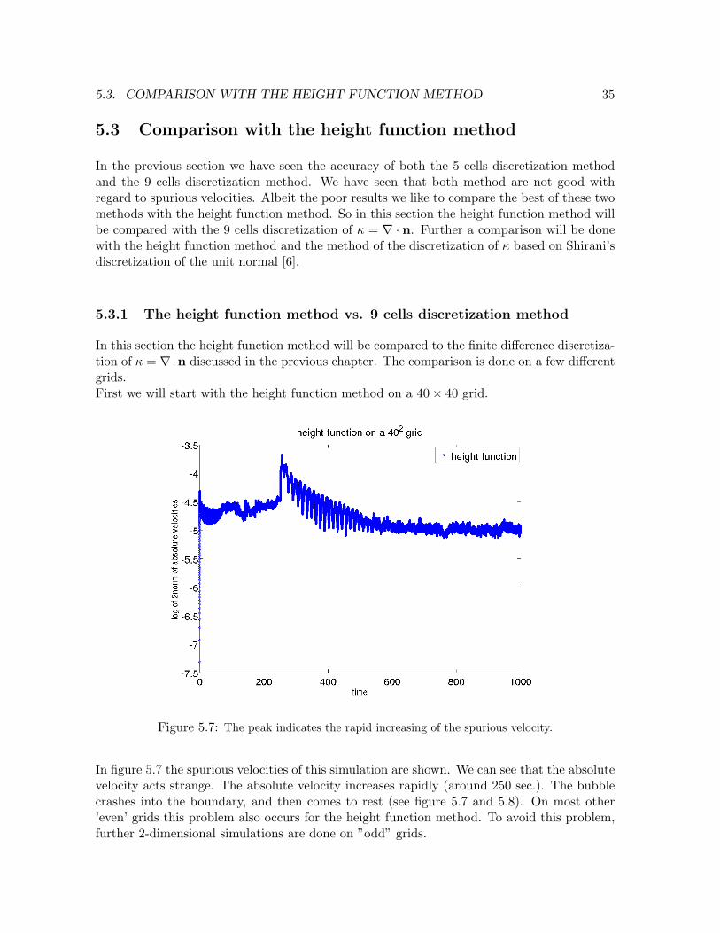
In this section the height function method will be compared to the finite difference discretiza-tion of κ = ∇·n discussed in the previous chapter. The comparison is done on a few differentgrids.First we will start with the height function method on a 40× 40 grid.
Figure 5.7: The peak indicates the rapid increasing of the spurious velocity.
In figure 5.7 the spurious velocities of this simulation are shown. We can see that the absolutevelocity acts strange. The absolute velocity increases rapidly (around 250 sec.). The bubblecrashes into the boundary, and then comes to rest (see figure 5.7 and 5.8). On most other’even’ grids this problem also occurs for the height function method. To avoid this problem,further 2-dimensional simulations are done on ”odd” grids.
36 CHAPTER 5. RESULTS
0 sec. 240 sec. 1000 sec.
Figure 5.8: The bubble crashes into wall.
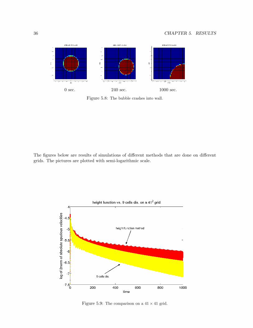
The figures below are results of simulations of different methods that are done on differentgrids. The pictures are plotted with semi-logarithmic scale.
Figure 5.9: The comparison on a 41× 41 grid.
5.3. COMPARISON WITH THE HEIGHT FUNCTION METHOD 37
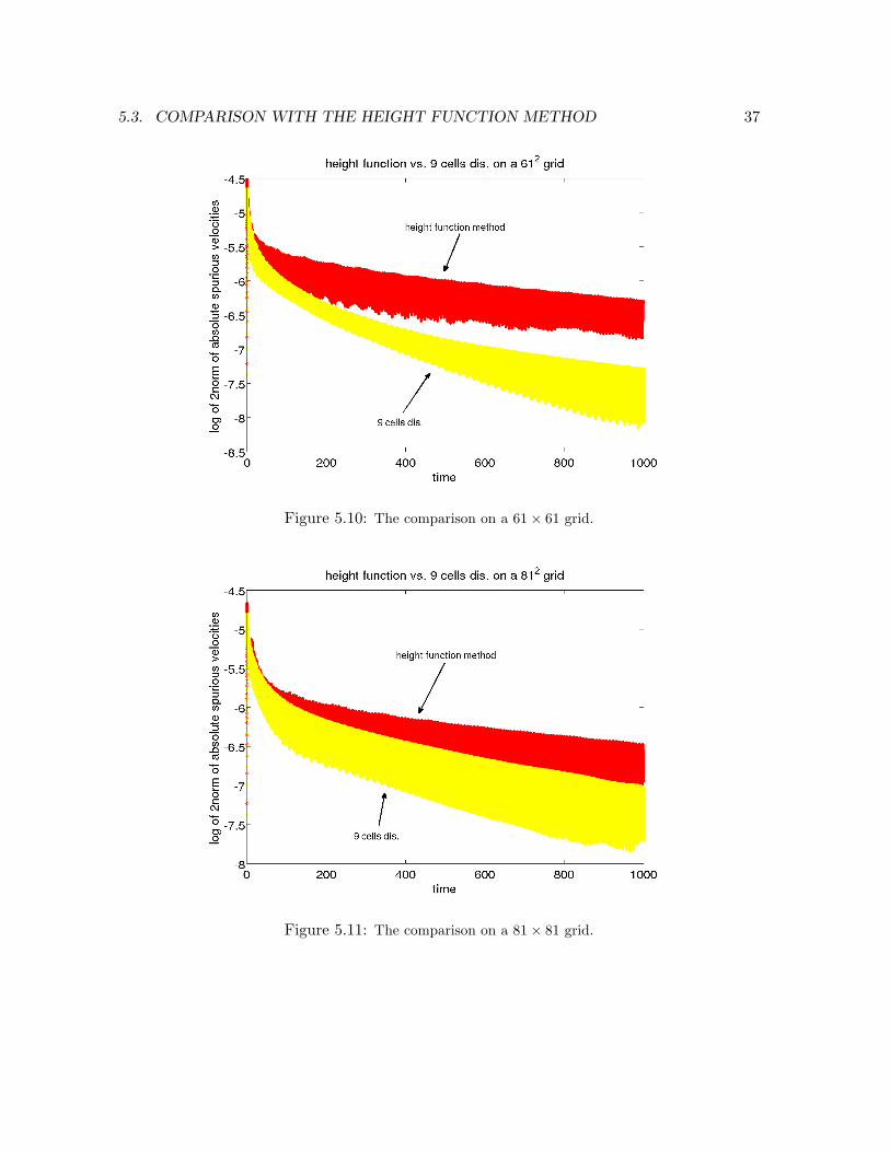
Figure 5.10: The comparison on a 61× 61 grid.
Figure 5.11: The comparison on a 81× 81 grid.
38 CHAPTER 5. RESULTS
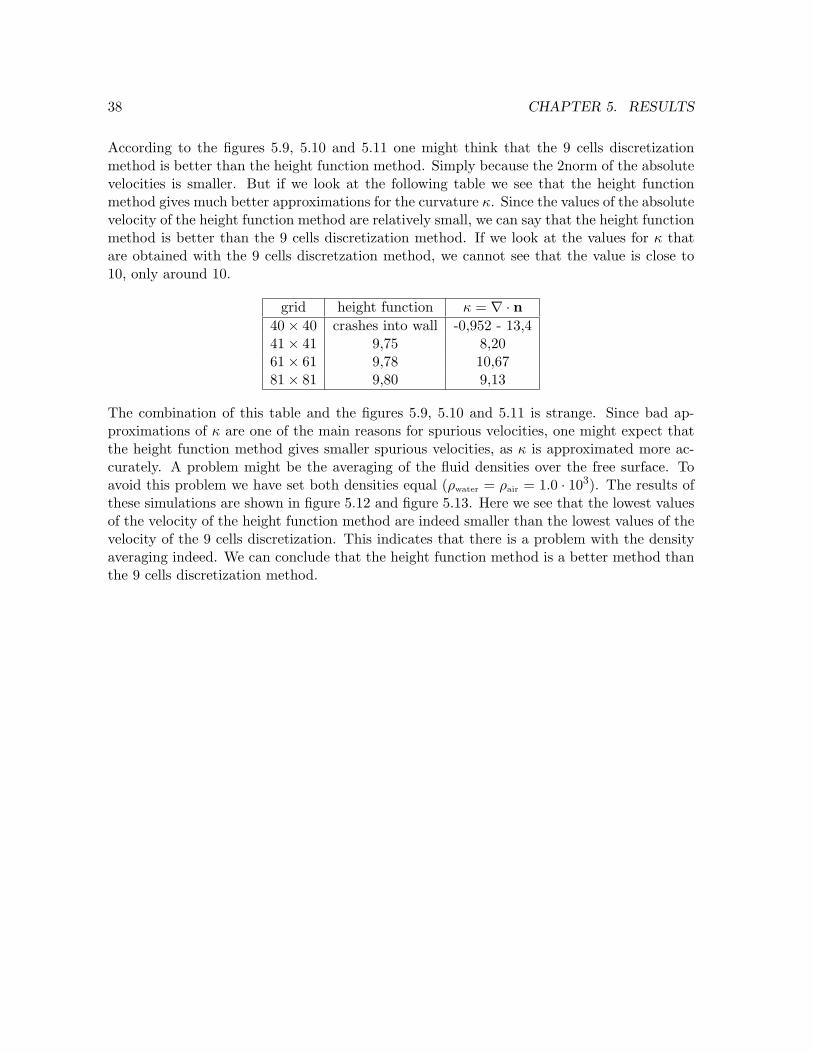
According to the figures 5.9, 5.10 and 5.11 one might think that the 9 cells discretizationmethod is better than the height function method. Simply because the 2norm of the absolutevelocities is smaller. But if we look at the following table we see that the height functionmethod gives much better approximations for the curvature κ. Since the values of the absolutevelocity of the height function method are relatively small, we can say that the height functionmethod is better than the 9 cells discretization method. If we look at the values for κ thatare obtained with the 9 cells discretzation method, we cannot see that the value is close to10, only around 10.
grid height function κ = ∇ · n40× 40 crashes into wall -0,952 - 13,441× 41 9,75 8,2061× 61 9,78 10,6781× 81 9,80 9,13
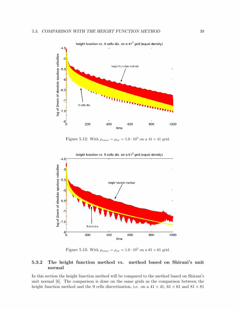
The combination of this table and the figures 5.9, 5.10 and 5.11 is strange. Since bad ap-proximations of κ are one of the main reasons for spurious velocities, one might expect thatthe height function method gives smaller spurious velocities, as κ is approximated more ac-curately. A problem might be the averaging of the fluid densities over the free surface. Toavoid this problem we have set both densities equal (ρwater = ρair = 1.0 · 103). The results ofthese simulations are shown in figure 5.12 and figure 5.13. Here we see that the lowest valuesof the velocity of the height function method are indeed smaller than the lowest values of thevelocity of the 9 cells discretization. This indicates that there is a problem with the densityaveraging indeed. We can conclude that the height function method is a better method thanthe 9 cells discretization method.
5.3. COMPARISON WITH THE HEIGHT FUNCTION METHOD 39
Figure 5.12: With ρwater = ρair = 1.0 · 103 on a 41× 41 grid.
Figure 5.13: With ρwater = ρair = 1.0 · 103 on a 61× 61 grid.
5.3.2 The height function method vs. method based on Shirani’s unitnormal
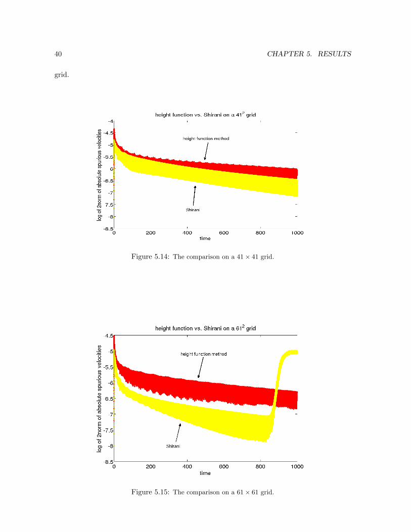
In this section the height function method will be compared to the method based on Shirani’sunit normal [6]. The comparison is done on the same grids as the comparison between theheight function method and the 9 cells discretization, i.e. on a 41× 41, 61× 61 and 81× 81
40 CHAPTER 5. RESULTS
grid.
Figure 5.14: The comparison on a 41× 41 grid.
Figure 5.15: The comparison on a 61× 61 grid.
5.3. COMPARISON WITH THE HEIGHT FUNCTION METHOD 41
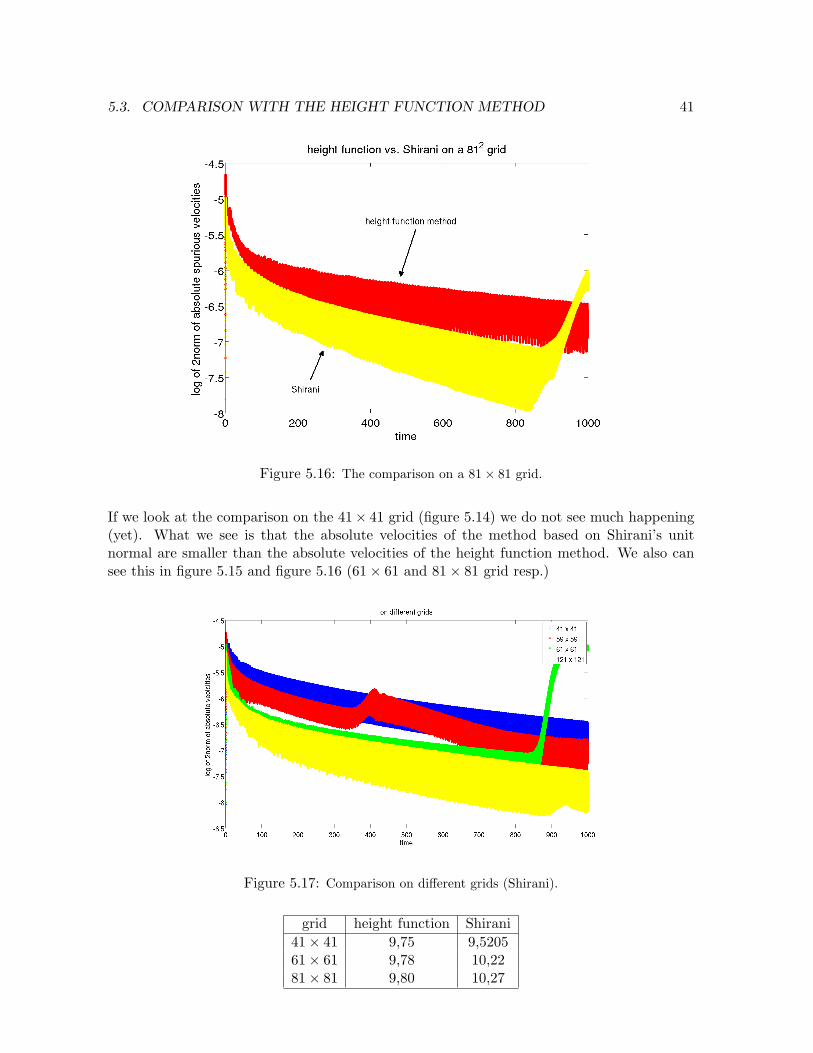
Figure 5.16: The comparison on a 81× 81 grid.
If we look at the comparison on the 41× 41 grid (figure 5.14) we do not see much happening(yet). What we see is that the absolute velocities of the method based on Shirani’s unitnormal are smaller than the absolute velocities of the height function method. We also cansee this in figure 5.15 and figure 5.16 (61× 61 and 81× 81 grid resp.)
Figure 5.17: Comparison on different grids (Shirani).
grid height function Shirani41× 41 9,75 9,520561× 61 9,78 10,2281× 81 9,80 10,27
42 CHAPTER 5. RESULTS
In figure 5.15 and figure 5.16 we see that the velocities of the ’Shirani methods’ are increas-ing rapidly around 820 seconds. We have looked at this problem. During our simulations,whether we have set the timestep δt such that the CFL-condition is obeyed, or the capillarytimestep is used. The sudden increase of the spurious velocity still occurs. The reason of thisremains unknown.
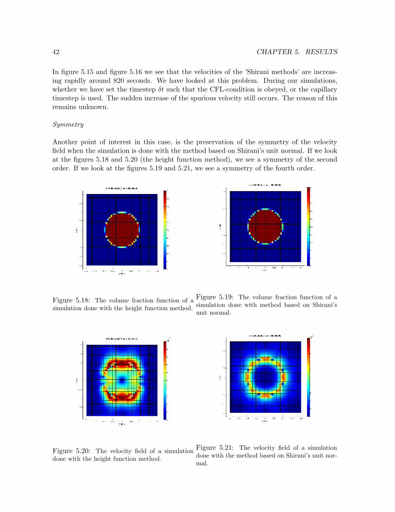
Symmetry
Another point of interest in this case, is the preservation of the symmetry of the velocityfield when the simulation is done with the method based on Shirani’s unit normal. If we lookat the figures 5.18 and 5.20 (the height function method), we see a symmetry of the secondorder. If we look at the figures 5.19 and 5.21, we see a symmetry of the fourth order.
Figure 5.18: The volume fraction function of asimulation done with the height function method.
Figure 5.19: The volume fraction function of asimulation done with method based on Shirani’sunit normal.
Figure 5.20: The velocity field of a simulationdone with the height function method.
Figure 5.21: The velocity field of a simulationdone with the method based on Shirani’s unit nor-mal.
5.4. RESULTS OF 3D METHODS 43
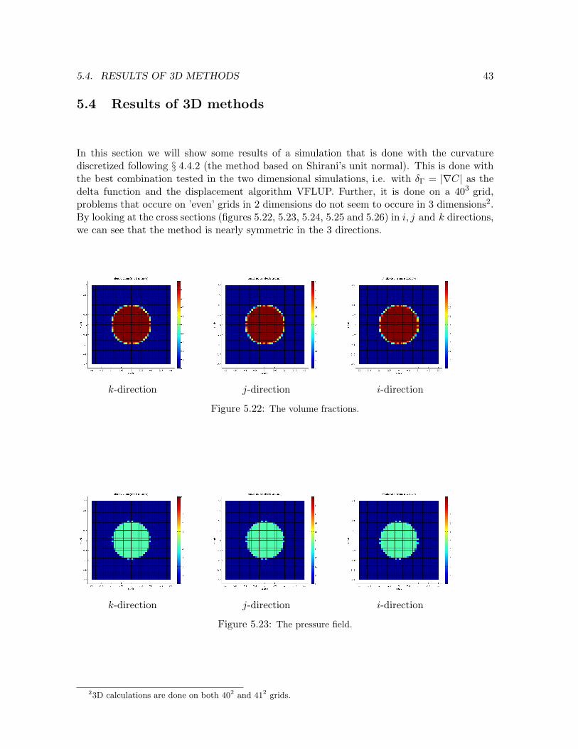
5.4 Results of 3D methods
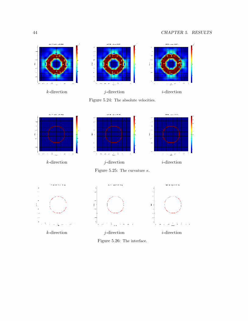
In this section we will show some results of a simulation that is done with the curvaturediscretized following § 4.4.2 (the method based on Shirani’s unit normal). This is done withthe best combination tested in the two dimensional simulations, i.e. with δΓ = |∇C| as thedelta function and the displacement algorithm VFLUP. Further, it is done on a 403 grid,problems that occure on ’even’ grids in 2 dimensions do not seem to occure in 3 dimensions2.By looking at the cross sections (figures 5.22, 5.23, 5.24, 5.25 and 5.26) in i, j and k directions,we can see that the method is nearly symmetric in the 3 directions.
k-direction j-direction i-direction
Figure 5.22: The volume fractions.
k-direction j-direction i-direction
Figure 5.23: The pressure field.
23D calculations are done on both 402 and 412 grids.
44 CHAPTER 5. RESULTS
k-direction j-direction i-direction
Figure 5.24: The absolute velocities.
k-direction j-direction i-direction
Figure 5.25: The curvature κ.
k-direction j-direction i-direction
Figure 5.26: The interface.
5.4. RESULTS OF 3D METHODS 45
In figure 5.25 we can see that the curvatures in the surface cells more or less have the samevalues. The mean value of the curvature κ = 19.8370, which is close to the real value of 20,
since in 3 dimensions κ =2r
holds for a bubble, and the rbubble = 0.1.
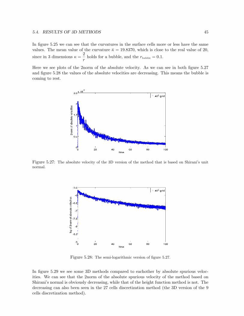
Here we see plots of the 2norm of the absolute velocity. As we can see in both figure 5.27and figure 5.28 the values of the absolute velocities are decreasing. This means the bubble iscoming to rest.
Figure 5.27: The absolute velocity of the 3D version of the method that is based on Shirani’s unitnormal.
Figure 5.28: The semi-logarithmic version of figure 5.27.
In figure 5.29 we see some 3D methods compared to eachother by absolute spurious veloc-ities. We can see that the 2norm of the absolute spurious velocity of the method based onShirani’s normal is obviously decreasing, while that of the height function method is not. Thedecreasing can also been seen in the 27 cells discretization method (the 3D version of the 9cells discretization method).
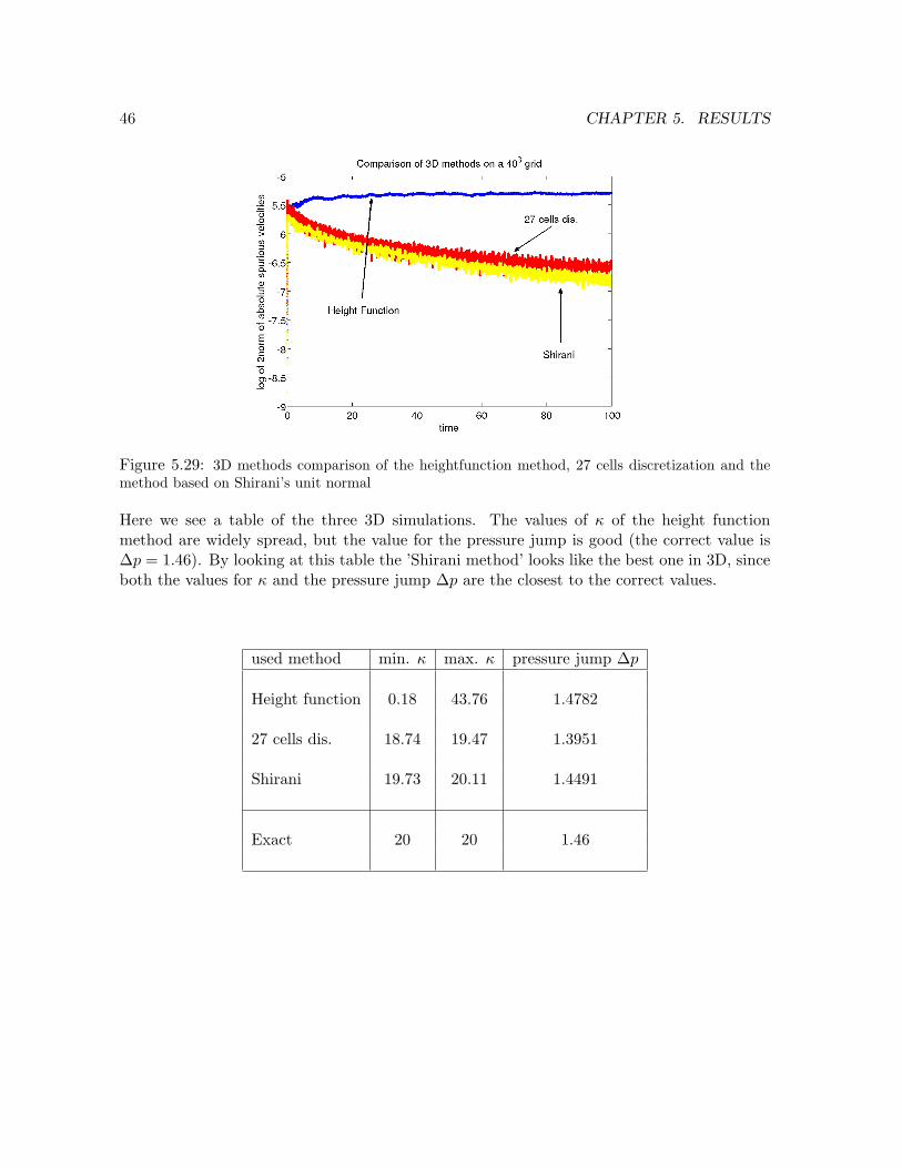
46 CHAPTER 5. RESULTS
Figure 5.29: 3D methods comparison of the heightfunction method, 27 cells discretization and themethod based on Shirani’s unit normal
Here we see a table of the three 3D simulations. The values of κ of the height functionmethod are widely spread, but the value for the pressure jump is good (the correct value is∆p = 1.46). By looking at this table the ’Shirani method’ looks like the best one in 3D, sinceboth the values for κ and the pressure jump ∆p are the closest to the correct values.
used method min. κ max. κ pressure jump ∆p
Height function 0.18 43.76 1.4782
27 cells dis. 18.74 19.47 1.3951
Shirani 19.73 20.11 1.4491
Exact 20 20 1.46
Chapter 6
Conclusion
In this study we have done simulations with a surface tension model (chapter 2). It is knownfrom literature that one of the main reasons for spurious currents to exist, is badly approxi-mated surface curvatures κ. Brackbill et al. [1] first mollifies the volume fraction function C,and then discretize this mollified function C with a finite difference method. The mollificationis necessary for the original volume fraction function C is too abrupt for a finite differencemethod (see figure 3.2). This method is used widely.But because the pressure gradient in the Navier-Stokes equation shows exact the same abrupt-ness as the volume fraction function C, we thought it would be interesting to see what willhappen if we leave C unmollified. In this study we have investigated a few discretizations ofthe curvature κ. Also we have used another delta function, for as we have seen in § 3.7 there
was missing a factor1m
in the method using delta function δΓ = 4C(1− C) when looking atthe equations, so this method is not expected to work well. This is comfirmed in § 5.1. Wesaw obvious movements of the bubble, and the spurious velocities were not decreasing, so thebubble will keep on moving and eventually crashes onto the boundary.Because of this reason further simulations were done with another delta function. We havechosen δΓ = |∇C|, as the units are matching when using this deltafunction. After many simu-lations we can conclude that VFLUP is a better displacement algorithm than VFCONV (seefigure 4.19 and 4.20). So all simulations are done with deltafunction |∇C| and displacementalgorithm VFLUP unless stated otherwise.First we have compared the 5 cells discretization of the curvature κ with the 9 cells discretiza-tion. The 5 cells discretization turned out to be inaccurate. A cause can be that too manycells are omitted in the 5 cells discretization (see figure 4.3 and figure 4.4). The four ”obvi-ous” cells were added to obtain a 9 cells discretization. In figure 5.5 and figure 5.6 we can seethat the spurious velocities of the 9 cells discretization method are smaller. The values of thecurvature κ of the 9 cells discretization are better, but unfortunately far from convincing.To see how good the 9 cells discretization method actually is, we have compared it to theheight function method, which is a well-known method for approximating κ [8]. In § 5.3.1we have compared both methods. At first glance, the 9 cells discretization method looks likea better method than the height function method, just by looking at the spurious velocitiesof both methods. But if we look at the values of the curvature the height function methodis much better. This is awkward, since the values of the spurious velocities are worse. Wesuspected that this is caused by the averaging of the densities of the fluid, and tested it withρwater = ρair = 1.0 · 103. As a result the minimum values for the spurious velocities are smaller
47
48 CHAPTER 6. CONCLUSION
with the height function method. We can say that the height function method is better thanthe 9 cells discretization method.Another discretization that we’ve investigated is based on the way the unit normal is dis-cretized by Shirani et al. [6]. We have also compared this method to the height functionmethod (the figures of this comparison are in § 5.3.2). We saw that the method based onShirani’s unit normal has smaller spurious velocities than the height function method till acertain time, but then suddenly the spurious velocities increase rapidly. Untill the suddenincrease of the velocities the method based on Shirani’s unit normal seems a better methodthan the height function method. If we look at the values of the curvature κ, they are notworse than the values that are obtained with the height function method. If we look at thesymmetry of the velocity field and volume fraction function (see figure 5.18, 5.19, 5.20 and5.21) we see that the method based on Shirani’s unit normal produces much nicer symmetry.So until the strange rapid increasing of the spurious velocity the method based on Shirani’sunit normal looks better. We do not have an idea what causes this problem.We have also done some simulation in 3D. In § 5.4 we see that ’Shirani’s method’ is nicelysymmetric in 3 directions. We have also compared several methods on a 40 × 40 × 40 grid.On this grid ’Shirani’s method’ looks like to be the best method.

Bibliography
[1] J.U. Brackbill, D.B. Kothe, and C. Zemach. A continuum method for modeling surfacetension. J. Comput. Phys., 100: 335-354, 1992
[2] B. Meier, G. Yadigaroglu, B.L. Smith. A novel technique for including surface tension inPLIC-VOF methods. Eur. J. Mech. B/Fluids., 21: 61-73, 2002
[3] A.E.P. Veldman, J. Gerrits, R. Luppes, J.A. Helder, J.P.B. Vreeburg. The numericalsimulation of liquid sloshing on board spacecraft. J. Comput. Phys., 224: 82-99, 2007
[4] S. Popinet, S. Zaleski. A front-tracking algorithm for accurate representation of surfacetension. Int. J. Numer. Fluids, 30: 75-793, 1999
[5] K.M.T. Kleefsman, G. Fekken, A.E.P. Veldman, B. Iwanowski, B. Buchner. A volume-of-Fluid based simulation for wave impact problems. J. Comput. Phys., 206: 363-393,2005
[6] E. Shirani, N. Ashgriz, J. Mostaghimi. Interface pressure calculation based on conserva-tion of momentum for front capturing methods. J. Comput. Phys., 203: 154-175, 2005
[7] M.W. Williams, D.B. Kothe, E.G. Puckett. Accuracy of Convergence of ContinuumSurface Tension Models, 1998
[8] M. ten Caat. Numerical Simulation of Incompressible Two-Phase Flow, Master’s Thesis.Groningen University, September 2002
[9] S. Afkhami and M. Bussmann. Height functions for applying contact angles to 3D VOFsimulations. Int. J. Numer. Meth. Fluids, 57: 453 - 472
[10] M. Raessi, J. Mostaghimi, M. Bussmann. Advecting normal vectors. A new method forcalculating interface normals and curvatures when modeling two-phase flows. J. Comput.Phys., 226: 774-797, 2007
[11] M.M. Francois, S.J. Cummins, E.D. Dendy, D.B. Kothe, J.M. Sicilian, M.W. Williams.A balanced-force algorithm for continuous and sharp interfacial surface tension modelswithin a volume tracking framework. J. Comput. Phys., 213: 141-173, 2006
[12] C.W. Hirt, D.B. Nichols. Volume of Fluid (VOF) Method for the Dynamics of FreeBoundaries. J. Comput. Phys., 39: 201-225, 1981
49