Laird Van Damme Ian Gillies Shawn Mizon Brad Chaulk Arnold Rudy Ben Kuttner Katelyn B. Loukes

2

Aerial Mapping 1920s

Aerial Photography 1940s…FRI 1960s

Satellite Imagery 1970s-present (e.g. Landcover 28)

Digital Aerial Imaging late 1990s….eFRI 2005

Active Sensors 2000s(e.g. LiDAR, RADAR)

3

4

NRCAN

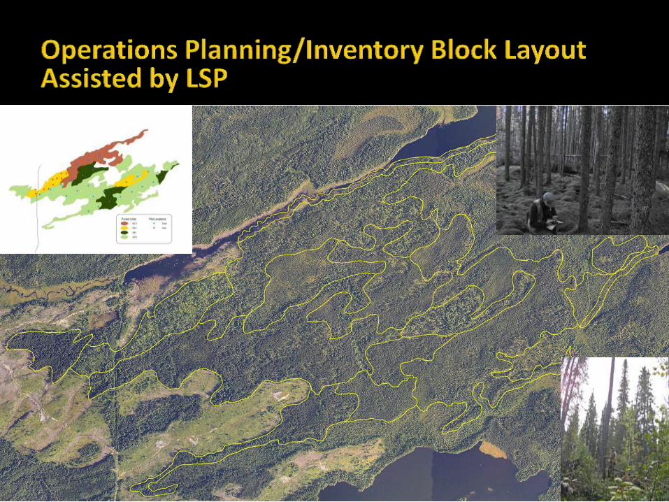
•Remote Sensing Used for Maps, Stratification and Interpretation •Location Most Important Value versus volume (plot based CFI in US and Europe)

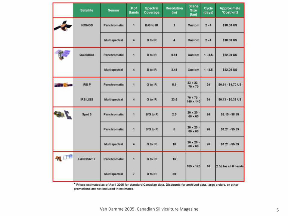
5 Van Damme 2005. Canadian Siliviculture Magazine

< 1 m

20-30 m

250 m

< 10 m

spat

ial r

eso

luti

on

low

high Orthophotos 30 cm (base data layer)

Landsat 30 m – (1/2 ha changes can be detected

MODIS 250 m

Source: MNR

Standard set 1961 SFLS > Innovation

Grid ( CFI ) LiDAR Softcopy

2004 MNR > ADS 40 A few minutes per stand SFMM Pinto Stand by Stand variance in leading species ( 60% correct) ADS 40 bandwidth will help improve species calls and heights (

X.Y.Z) Bowater Grid> Growing Stock and Species comp good Age> Not

so good> KBM/U of T research Ben Kuttner)

7

13

Lu CARIS/KBM Research

ITC Segmentation and

object-based classification

Cloud computing

(Bergeron et al. 2002, Nguyen 2000; 2002)

Rotation age under traditional even-aged management

Stand age estimates are relied upon to estimate volumes and to associate wildlife habitat values with stands, present and future

In many circumstances photo interpreted stand age estimates based on dominant and co-dominant trees fail to reflect stand structural conditions e.g., two-tiered stands vs. single cohort vs. complex

multicohort stands that may all get similar age estimates based on estimated age of dominants

Where possible, does it not make sense to measure stand structural complexity to complement stand age estimates ?

better volume estimates, growth estimates, etc.

ability to estimate piece size distributions

more precise measurement of habitat conditions

means to ensure the intent of age-based guidelines for maintaining structure and function are met.

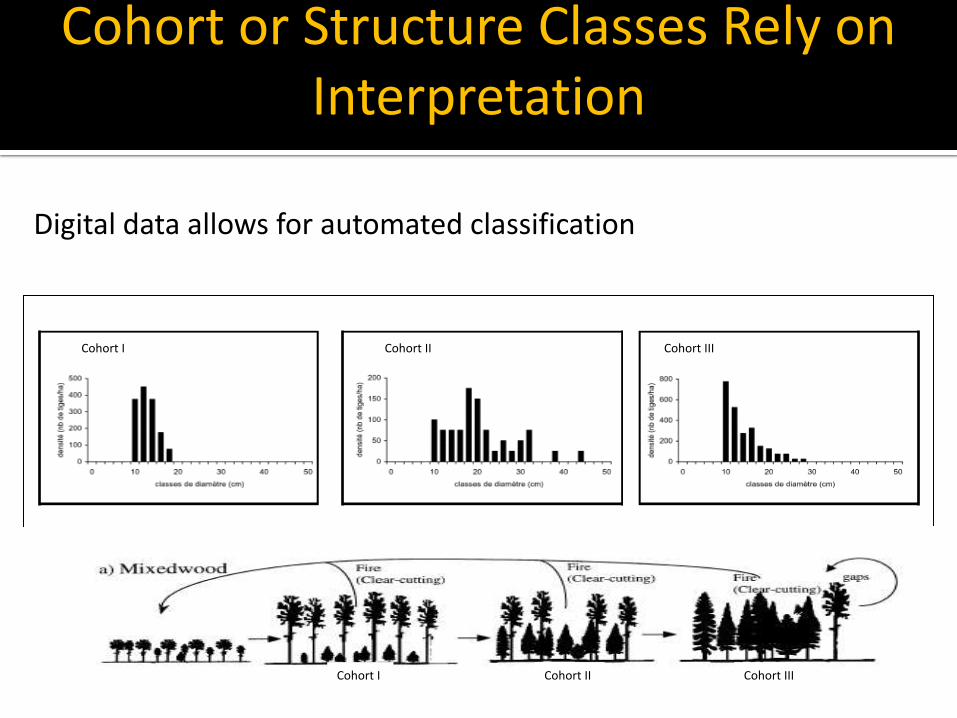
Digital data allows for automated classification

(adapted from Boucher et al. 2003, Nguyen 2002)

Cohort I Cohort II Cohort III

Cohort I Cohort II Cohort III

Cohort or Structure Classes Rely on Interpretation

Airborne Laser Scanner (ALS) - Small footprint discrete return light detection and ranging (LiDAR):

Woods (MNR)

usgs.gov

msstate.edu

Stand Age = 109 SF1; Class = 3

MW2 & SF1 Results

PCA 1 (37%)

-1.5 -1.0 -0.5 0.0 0.5 1.0 1.5

PC

A 2

(3

1%

)

-1.5

-1.0

-0.5

0.0

0.5

1.0

1.5

DTOT

Dlpct

Dmpct

Dspct

Skew

CV

S

H

E

rangedbh maxdbhc

w_scale

w_shape

CCR

CCH CCE

Cohort III

Cohort IICohort I

LEGEND Diameter class variables H - diversity E - eveness S - richness Skew - coefficient of skewness CV - coefficient of variation W_scale - Weibull (W.) scale W_shape – W. shape parameter Crown class (CC) variables CCE - eveness CCR - richness CCH – diversity Tree density variables Dspct - % 2.5-9.0 cm DBH Dmpct - % 9.0-21.0 cm DBH Dlpct% - > 21.0 cm DBH DTOT - Total trees/ha Disturbance History Symbols ■ = logged ● = un-logged natural

▲ = unknown

MWSF MEAN WEIBULL CURVES

DBH (cm)

0 20 40 60

Tre

e d

ensity (

%)

0

5

10

15

20

25

Class 1

Class 2

Class 3

TEM-01-090

0

200

400

600

800

1000

2 6 10 14 18 22 26 30 34 38 42

DBH class (cm)

Tre

es/h

a

TEM-01-085

0

200

400

600

800

1000

2 6 10 14 18 22 26 30 34 38 42

DBH class (cm)

Tre

es/h

a

TEM-01-095

0

200

400

600

800

1000

2 6 10 14 18 22 26 30 34 38 42

DBH class (cm)

Tre

es/h

a

Class 1 Mixedwood

Class 2 Mixedwood

Class 3 Mixedwood

Class 1 Black Spruce

SB1 Class 2

TEM-01-019

0

500

1000

1500

2000

2500

2 4 6 8 10 12 14 16 18 20 22 24 26

DBH class (cm)

Tre

es/h

a

TEM-01-034

0

500

1000

1500

2000

2500

2 4 6 8 10 12 14 16 18 20 22 24 26

DBH class (cm)

Tre

es/h

a

TEM-01-036

0

500

1000

1500

2000

2500

2 4 6 8 10 12 14 16 18 20 22 24 26

DBH class (cm)

Tre

es/h

a

Class 2 Black Spruce

Class 3 Black Spruce

• The distribution of height returns (left) reflects differences in diameter distributions (right) among cohorts at the 400 m2 plot scale

• Discriminant classification function models can be used to select return height distribution summary variables to predict cohort structure class

DBH class

0 10 20 30 40

Tre

es/h

a

0

200

400

600

800

1000

CHT512 Stand Age = 109 SF1; Class = 3

Cohort Classification using ALS LiDAR

Class 3 Mixedwood

Class 2 Mixedwood

Class 1 Mixedwood

Automatic Point Cloud Extraction: Software

Inpho Match-T DSM Parallax Pixel-based matching Uses multiple overlapping

images (stereomodels) “Robust Filtering

Techniques” DTM Toolkit – Classifies and

filters ground, vegetation and buildings Modified from Wu et. al. 2004

25

A comparison of LiDAR point clouds (left), ADS40 imagery-derived point clouds (middle) and ADS40 imagery (KBM U of T IRAP)

• Colour gradient represents height differences in point heights between photogtrammetry point cloud and Lidar point cloud • Note time lag between LiDAR and ADS40 4-5 yrs. •Largest differences seen in open, quickly regenerating areas (roadsides, cutovers)

0

5

10

15

20

25

30

P1 P5 P10 P25 P50 P75 P90 P95 P99

Me

an 2

0x2

0m

Gri

d P

erc

en

tile

He

igh

t (m

)

Percentile

Inpho Height

LiDAR Height

Advances in Digital Photogrammetry

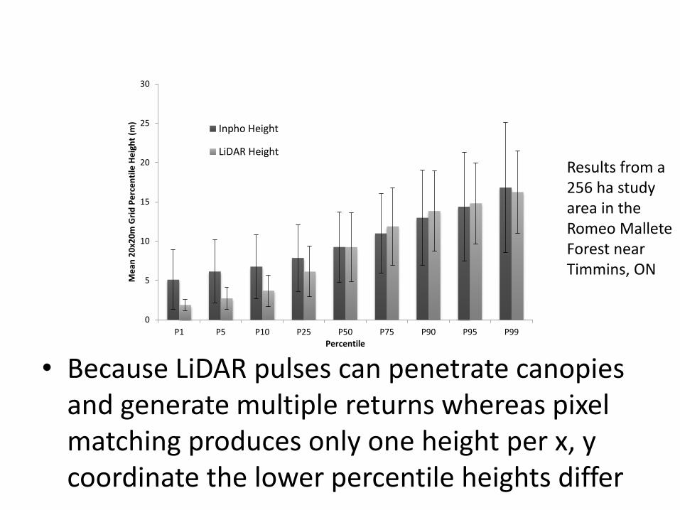
• Because LiDAR pulses can penetrate canopies and generate multiple returns whereas pixel matching produces only one height per x, y coordinate the lower percentile heights differ

Results from a 256 ha study area in the Romeo Mallete Forest near Timmins, ON

Despite the limitations of imagery point clouds compared to LiDAR point clouds we believe cohort classification using INPHO point clouds may be possible.

Cohort Classification Using Digital Photogrammetry

• Why? because imagery-derived point clouds accurately measure heights in upper canopy strata. Horizontal and vertical variability in upper canopy point heights are key variables

29

30

LiDAR/imagery combo more common

Greater precision xyz possible but at greater cost.

Sensors are providing a wider range of wave length and increased accuracies at lower costs as technology advances

Create DEM using LiDAR Maintain FRI using DSMs from:

Satellite ( 50 cm stereo launched in 2013 $10MM)

ADS 40 (Band width advantage)

Digital Camera ( Point cloud advantage depending on resolution)

Photo-LiDAR

▪ Whatever is most cost effective

31

32

33

34

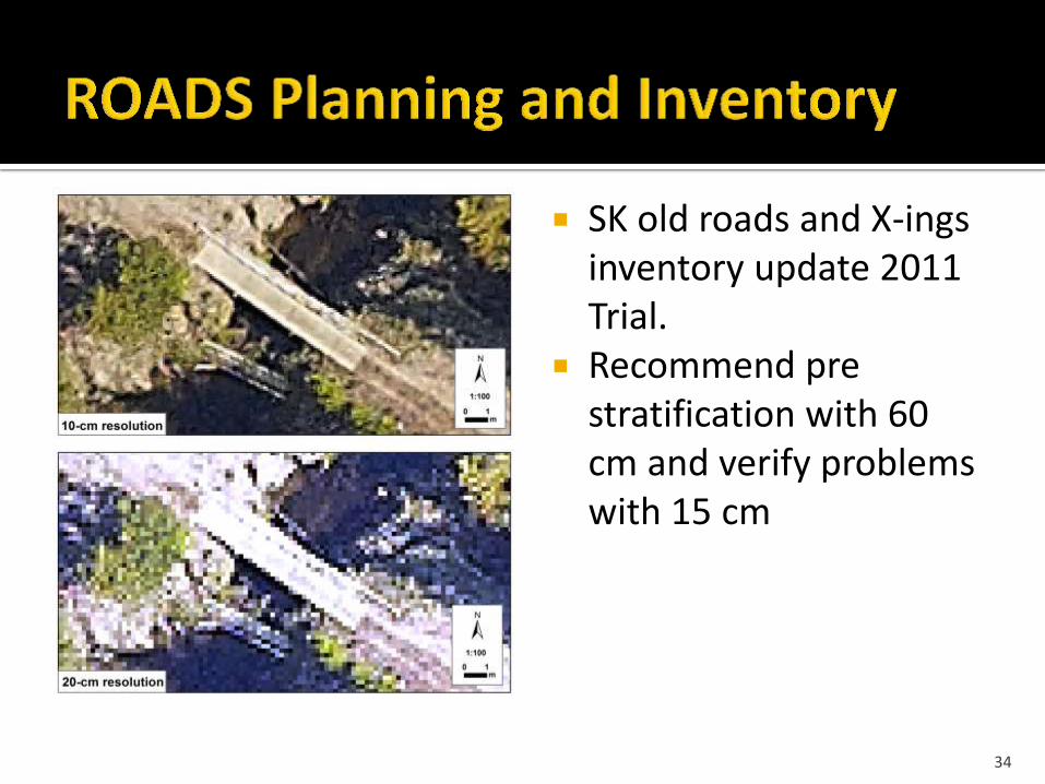
SK old roads and X-ings inventory update 2011 Trial.

Recommend pre stratification with 60 cm and verify problems with 15 cm

35

AB use of LSP for compliance tendered out 2010

Opportunities in ON

Utilization

Water crossings

Retention

Stump Heights

Rutting

Aggregate Pits

36

37

Dendron 1980-2010 35-70 mm LSPs Timber Appraisal FTG

R&B Cormier 2000-2010 70mm Boom-mounted Helicopter

Platform FTG

KBM/LU CARIS 1996-2011 Partnership program for

applied research Fixed wing Small format digital FTG

38

Low cost alternative to rotary wing platform

Digital technology improving rapidly

3-6 cm resolution available fixed wing

Survey grade 1-2 cm available UAVs

39

More reliable and less expensive than comparable satellite imagery

Dispersion of cut-blocks

Fixed orbit of satellites

Cloud cover

Data collection can be timed to coincide with weather windows

40

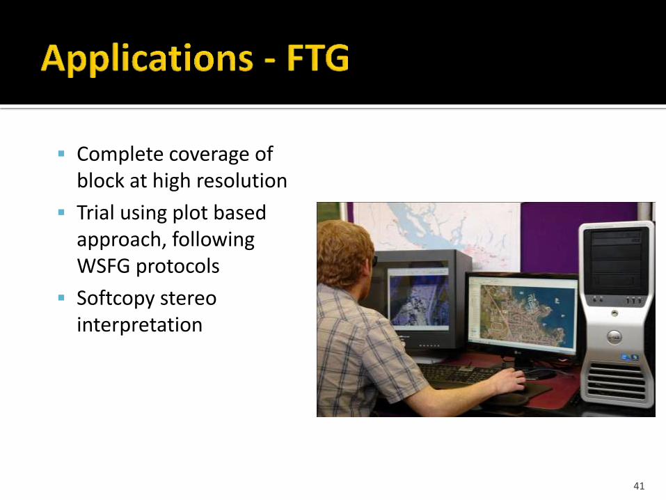
Complete coverage of block at high resolution

Trial using plot based approach, following WSFG protocols

Softcopy stereo interpretation

41

Observations compared to field plots

Heights – good agreement

Species compositions were very similar, especially on leading species

LSP underestimated stems/ha

LSP WSFG stocking estimates varied – likely based on actual plot locations, small stems

Ground sampling and existing records always helpful and necessary in some cases to make best call possible

80k ha in 2011

42

Considerable interest from licensees

Lower cost than ground survey

Permanent, repeatable, verifiable record

Additional benefits of imagery (e.g. boundary update)

Satisfies reporting and planning requirements(???)

Leaf-off conditions critical for success in most cases

Obviously more information is better

All available records, ground work,etc.

Working with licensee more efficient

43

Ground surveys may or may not still be needed

Still provides substantial information in all situations

Stratify to focus field efforts where required

Some silvicultural ground rules may have to be revisited to accommodate this system

44

No system is perfect WSFG Bw9 Sb1 LSP-specific protocols?

Aerial versus ground won’t match in all situations

FRI is pps (baf 2 m2/ha) FTG also pps?

45

Comes down to cost, risk, and value

Ocular assessments high risk

WSFG or similar high cost

LSP high value

Medium Cost/Risk alternative

Permanent record (auditable)

Not limited to FTG, revisit for other information

Growing use/acceptance (e.g. AB/SK)

46

Aerial imaging and associated technologies advancing quickly

Costs trending down ▪ Example, LiDAR 4x increase in resolution and 50% reduction in costs

over 5 years

Spatial coverage at given resolution increasing

Spectral coverage likely to follow

Becoming more manageable to process/store/access data

Point cloud data can help in segmentation and classification

47

Normalized Ht (m)

Height (m) >

Las Tools

Inpho-Fast

> >

Height (m)

Inpho-Scop

50

51

52

53

LU-CARIS;

Dr. Ulf Runesson

U of T:

Dr. Jay Malcolm; Dr Ben Kuttner; Katelyn Loukes

OCE

Richard Worsfold

NSERC IRAP;

Paul Tulanen

54