Available online at www.sciencedirect.com

ScienceDirect

Comput. Methods Appl. Mech. Engrg. 281 (2014) 106–130www.elsevier.com/locate/cma

Nonlinear performance of continuum mechanics based beamelements focusing on large twisting behaviors

Kyungho Yoon, Phill-Seung Lee∗

Division of Ocean Systems Engineering, Korea Advanced Institute of Science and Technology, 291 Daehak-ro, Yuseong-gu,Daejeon 305-701, Republic of Korea

Received 10 May 2014; received in revised form 2 July 2014; accepted 23 July 2014Available online 1 August 2014

Abstract

In this paper, we present the nonlinear formulation and performance of continuum mechanics based beam elements, in whichfully coupled 3D behaviors of stretching, bending, shearing, twisting, and warping are automatically considered. The beamelements are directly degenerated from assemblages of 3D solid elements under the assumptions of Timoshenko beam theory.Therefore, cross-sectional discretization is possible and the elements can model complicated 3D beam geometries including curvedand twisted geometries, varying cross-sections, eccentricities, and arbitrary cross-sectional shapes. In particular, the proposednonlinear formulation can accurately predict large twisting behaviors coupled with stretching, bending, shearing, and warping.Through various numerical examples, we demonstrate the geometric (and material) nonlinear performance of the continuummechanics based beam elements.c⃝ 2014 Elsevier B.V. All rights reserved.

Keywords: Nonlinear analysis; Finite element method; Beam element; Large twisting; Warping; Lateral buckling

1. Introduction

Beams are widely used structural members in various engineering fields including marine, mechanical, civilengineering, and aerospace engineering fields [1–5]. Recently, beam applications have rapidly extended from classicalmetallic structures to nano- and bio-structures [6–8], in which the finite element method is a tool that has beendominantly adopted for analysis and design. In order to encompass these new applications, the modeling capabilityand nonlinear performance have become increasingly important in the finite element analysis of beams.

For a long time, considerable efforts have been made regarding beam theories and the development of beam finiteelements; see Refs. [2,3,9–20] for a review of the existing research. Based on classical beam theories, recent workshave focused on developing high performance beam finite elements for linear and nonlinear analyses. As a result,the modeling and analysis capabilities have been continuously improved; see Refs. [21–29] for examples. However,compared with other kinematics, relatively small improvements have been made in the large twisting kinematics ofbeams.

∗ Corresponding author. Tel.: +82 42 350 1512; fax: +82 42 350 1510.E-mail address: phillseung@kaist.edu (P.S. Lee).

http://dx.doi.org/10.1016/j.cma.2014.07.0230045-7825/ c⃝ 2014 Elsevier B.V. All rights reserved.

K. Yoon, P.S. Lee / Comput. Methods Appl. Mech. Engrg. 281 (2014) 106–130 107

It is well known that isoparametric beam elements are degenerated from 3D solid elements [1]. Because the beamelements are based on 3D continuum mechanics, they can easily represent general 3D curved geometries includingfully coupled complete strains, and the formulation is simple and straightforward. Despite these significant advantages,the original isoparametric beam elements can generally only consider rectangular cross-sections. While several studieshave been undertaken in attempts to overcome this limitation in the isoparametric beam elements [4,30–33,27,34], theresulting beams do not clearly model arbitrary beam cross-sections.

Recently, Yoon et al. [35] proposed the concept of continuum mechanics based beam elements, which are de-generated from assemblages of 3D solid elements. Therefore, these beam elements can be considered to be a directextension of isoparametric beam elements. However, unlike the isoparametric beam elements, the continuum mechan-ics based beam elements can easily model complicated 3D beam geometries including curved and twisted geometries,varying cross-sections, eccentricity, and arbitrary cross-sectional shapes by incorporating cross-sectional meshes. Fur-thermore, the beam elements can represent fully coupled behaviors among bending, shearing, stretching, twisting, andwarping.

The objective of this paper is to develop a general nonlinear formulation of continuum mechanics based beam ele-ments and present their nonlinear performance focusing on large twisting behaviors. The total Lagrangian formulationis employed and, unlike other beam elements [22–25], the Wagner effect is automatically (implicitly) considered inthe beam formulation due to the continuum mechanics based formulation, which results in the capability for largetwisting analyses.

The novel aspects of the proposed beam element formulation are summarized as follows:

• The formulation is simple and straightforward.• Seven degrees of freedom (DOFs) are used at each beam node in order to ensure the inter-elemental continuity of

the warping displacements.• The formulation can manage complicated 3D beam geometries including curved and twisted geometries, varying

cross-sections, eccentricity, and arbitrary cross-sectional shapes [35,36].• The complete tangent stiffness matrix is obtained because the finite rotation of the director vectors is precisely

included up to a quadratic order.• The large twisting and lateral buckling behaviors can be accurately calculated. In the Green–Lagrange strain, the

Wagner strain is included implicitly.

In the following sections, the nonlinear kinematics of the continuum mechanics based beams is described. Then,the strain measures are introduced from the given kinematic description and the assumed strain technique used forlocking reduction. Next, the incremental equilibrium equation is presented based on the total Lagrangian formulation.Finally, the novelties of the continuum mechanics based beam finite element are demonstrated using well establishednumerical examples that focus on large twisting behaviors.

2. Large displacement kinematics

The continuum mechanics based beam elements are degenerated from assemblages of 3D solid finite elements [35].In this section, the large displacement kinematics of the continuum mechanics based beams is presented. In thefollowing formulations, a superscript (or subscript) t is employed to denote time; however, in the static nonlinearanalyses considered in this study, t is a dummy variable that indicates the load levels and incremental variables ratherthan the actual time as in dynamic analyses [1].

Consider a q-node continuum mechanics based beam element that consists of n sub-beams in the configuration attime t , as depicted in Fig. 1. Allowing warping displacements, the geometry interpolation of the sub-beam m (shadedin Fig. 1) is given by

t x(m)=

qk=1

hk(r)t xk +

qk=1

hk(r)y(m)k

t Vky +

qk=1

hk(r)z(m)k

t Vkz +

qk=1

hk(r) f (m)k

tαkt Vk

x , (1)

in which t x(m) is the material position vector at time t , hk(r) is the 1D shape function at beam node k, t xk is theposition of beam node k at time t , t Vk

x ,t Vk

y , and t Vkz are the unit director vectors at time t and are normal to each

other, y(m)k and z(m)

k denote the position in the beam cross-section at beam node k, f (m)k is the warping function at

beam node k, and tαk is the corresponding warping degree of freedom at beam node k at time t ; see Refs. [35,36] for

108 K. Yoon, P.S. Lee / Comput. Methods Appl. Mech. Engrg. 281 (2014) 106–130

Fig. 1. A 3-node continuum mechanics based beam element with cross-sectional discretization in the configuration at time t . In this figure, thecontinuum mechanics based beam element consists of 9 sub-beams.

the detailed derivation of Eq. (1). Note that this type of warping model has an intrinsic drawback, that is, the inter-elemental continuity of warping cannot be properly satisfied at nodes where multiple elements are connected and anangle between adjacent elements is not small, see Ref. [28] and therein.

In the continuum mechanics based beam element, a beam cross-section is modeled using a cross-sectional mesh,which is defined using cross-sectional nodes and elements, as seen in Fig. 2. Considering the p-node cross-sectionalelement m (shaded in Fig. 2) that corresponds to the sub-beam m, the position and warping functions at beam node kare given by

y(m)k =

pj=1

h j (s, t)y j (m)k , z(m)

k =

pj=1

h j (s, t)z j (m)k , f (m)

k =

pj=1

h j (s, t) f j (m)k , (2)

where h j (s, t) is the 2D shape function, y j (m)k and z j (m)

k denote the position of the cross-sectional node j , and f j (m)k

is the warping value at cross-sectional node j . Note that the number of cross-sectional elements is equal to the numberof sub-beams.

In order to represent the material position in the beam cross-section at beam node k, the cross-sectional Cartesiancoordinate system is defined using the director vectors t Vk

y and t Vkz , and the origin Ck . Note that the position of beam

node k, t xk is located at the origin Ck . The warping director t Vkx in Eq. (1) denotes the warping direction at beam

node k at time t and is calculated using t Vkx =

t Vky ×

t Vkz . The warping values are pre-calculated through solving the

St. Venant equations using the finite element procedure with the given cross-sectional meshes, see Refs. [35,36] formore detailed discussions of this method.

For the sub-beam m, the incremental displacement is obtained from the configurations at time t and t + 1t , asfollows

0u(m)=

t+1t x(m)−

t x(m). (3)

K. Yoon, P.S. Lee / Comput. Methods Appl. Mech. Engrg. 281 (2014) 106–130 109

Fig. 2. A continuum mechanics based beam element: (a) beam nodes and coordinate systems used in the beam element and (b) cross-sectionalnodes and elements in the cross-sectional mesh.

Using Eq. (1) in Eq. (3), the interpolation of the incremental displacement is obtained by

0u(m)=

qk=1

hk(r)0uk +

qk=1

hk(r)y(m)k (t+1t Vk

y −t Vk

y) +

qk=1

hk(r)z(m)k (t+1t Vk

z −t Vk

z )

+

qk=1

hk(r) f (m)k (t+1tαk

t+1t Vkx −

tαkt Vk

x ), (4)

where 0uk is the incremental nodal displacement at beam node k from time t to t + 1t .For the parametrization of finite rotations [37–40], the well-known Rodrigues formula is used, as follows

R(0θk) = I +

sin 0θk

0θk R(0θk) +

1 − cos 0θk

0θk2 R(0θk)2 (5)

110 K. Yoon, P.S. Lee / Comput. Methods Appl. Mech. Engrg. 281 (2014) 106–130

with 0θk

=

0θ

kx 0θ

ky 0θ

kz

T, 0θ

k=

0θk2

x + 0θk2y + 0θk2

z ,

R(0θk) =

0 −0θkz 0θ

ky

0θkz 0 −0θ

kx

−0θky 0θ

kx 0

, (6)

where 0θkx , 0θ

ky , and 0θ

kz are the incremental Eulerian angles from time t to t + 1t , and R is the skew-symmetric

matrix operator.Then, the director vectors at time t + 1t are defined as

t+1t Vkx = R(0θ

k)t Vkx ,

t+1t Vky = R(0θ

k)t Vky, and t+1t Vk

z = R(0θk)t Vk

z . (7)

Using Eq. (7) in Eq. (4), we can obtain the following

0u(m)=

qk=1

hk(r)0uk +

qk=1

hk(r)y(m)k (R(0θ

k) − I)t Vky +

qk=1

hk(r)z(m)k (R(0θ

k) − I)t Vkz

+

qk=1

hk(r) f (m)k (0αkR(0θ

k) +tαk(R(0θ

k) − I))t Vkx , (8)

in which 0αk is the incremental warping degree of freedom at beam node k.Applying the Taylor expansion to Eq. (5), the finite rotation tensor R(0θ

k) can be represented using a polynomialfunction with respect to the incremental Eulerian angle vector 0θ

k

R(0θk) = I + R(0θ

k) +12!

R(0θk)2

+13!

R(0θk)3

+14!

R(0θk)4

+ · · · . (9)

Substituting Eq. (9) into Eq. (8) and using the second order approximation for the finite rotation, the incrementaldisplacement in Eq. (8) becomes

0u(m)≈ 0u(m)

1 + 0u(m)2 (10)

with

0u(m)1 =

qk=1

hk(r)0uk +

qk=1

hk(r)y(m)k R(0θ

k)t Vky +

qk=1

hk(r)z(m)k R(0θ

k)t Vkz

+

qk=1

hk(r) f (m)k [0αkI +

tαkR(0θk)]t Vk

x , (11)

0u(m)2 =

12

qk=1

hk(r)y(m)k R(0θ

k)2t Vky +

12

qk=1

hk(r)z(m)k R(0θ

k)2t Vkz

+

qk=1

hk(r) f (m)k

0αkR(0θ

k) +12

tαkR(0θk)2

t Vk

x , (12)

in which 0u(m)1 and 0u(m)

2 are the linear and quadratic parts, respectively, in the incremental displacement.In the incremental displacement in Eq. (10), seven DOFs (three translations, three rotations, and one warping DOF)

are employed at beam node k using the nodal DOFs vector:

0Uk =

0uk 0vk 0wk | 0θ

kx 0θ

ky 0θ

kz | 0αk

T, (13)

and the DOFs vector of the q-node beam element is as follows

0U =

0UT

1 0UT2 · · · 0UT

q

T. (14)

K. Yoon, P.S. Lee / Comput. Methods Appl. Mech. Engrg. 281 (2014) 106–130 111

Then, 0u(m)1 is represented in terms of the nodal DOFs vector

0u(m)1 =

L(m)

1 L(m)2 · · · L(m)

q

0U = L(m)

0U (15)

with

L(m)k = hk(r)

I −

y(m)

k R(t Vky) + z(m)

k R(t Vkz ) + f (m)

ktαkR(t Vk

x )

f (m)k (s, t)t Vk

x

. (16)

Also, 0u(m)2 is given by

0u(m)2 =

0u(m)2

0v(m)2

0w(m)2

=12

0UT1Q(m)

0U0UT

2Q(m)0U

0UT3Q(m)

0U

(17)

with

i Q(m)=

i Q

(m)1 i Q

(m)2 · · · i Q(m)

q

, i = 1, 2, 3, (18)

in which

i Q(m)k = hk(r)

0 0 00 y(m)

k ψi (t Vk

y) + z(m)k ψi (

t Vkz ) + f (m)

ktαkψi (

t Vkx ) − f (m)

k Ri (t Vk

x )T

0 − f (m)k Ri (

t Vkx ) 0

(19)

with

ψ1(x) =12

0 x2 x3x2 −2x1 0x3 0 −2x1

, ψ2(x) =12

−2x2 x1 0x1 0 x30 x3 −2x2

,

ψ3(x) =12

−2x3 0 x10 −2x3 x2x1 x2 0

, (20)

and

R1(x) =0 −x3 x2

, R2(x) =

x3 0 −x1

, and R3(x) =

−x2 x1 0

. (21)

The variations of the incremental displacements are given by:

δ0u(m)1 = L(m)δ0U and δ0u(m)

2 =

δ0u(m)

2

δ0v(m)2

δ0w(m)2

=

δ0UT1Q(m)

0Uδ0UT

2Q(m)0U

δ0UT3Q(m)

0U

. (22)

3. Green–Lagrange strains

The covariant Green–Lagrange strain tensor t0ε

(m)i j for the sub-beam m at the configuration at time t , referred to the

configuration at time 0, is defined as follows

t0ε

(m)i j =

12(t g(m)

i ·t g(m)

j −0g(m)

i ·0g(m)

j ) with t g(m)i =

∂ t x(m)

∂ri, (23)

in which r1 = 1, r2 = 2, and r3 = 3. Since cross-sectional deformations are not allowed in Timoshenko beam theory,in the beam formulation, only five strain components (t

0ε(m)11 , t

0ε(m)12 , t

0ε(m)21 , t

0ε(m)13 , and t

0ε(m)31 ) are considered; that is,

(i, j) ∈ {(1, 1), (1, 2), (2, 1), (1, 3), (3, 1)}. The other strain components (t0ε

(m)22 , t

0ε(m)33 , t

0ε(m)23 , and t

0ε(m)32 ) are zero.

It is important to note that, when the covariant base vector t g(m)i is calculated, the warping effect in the geometry

112 K. Yoon, P.S. Lee / Comput. Methods Appl. Mech. Engrg. 281 (2014) 106–130

interpolation in Eq. (1) should be considered. Otherwise, the Wagner strain term cannot be correctly included in thebeam formulation, see Appendix.

The local Green–Lagrange strain tensor t0ε

(m)i j defined in the local Cartesian coordinate system in Fig. 2(a) is

calculated using the following equation:

t0ε

(m)i j (0ti ⊗

0t j ) =t0ε

(m)kl (0gk(m)

⊗0gl(m)), (24)

where the base vectors for the local Cartesian coordinate system are given by:

0t1 = hk(r)0Vkx ,

0t2 = hk(r)0Vky and 0t3 = hk(r)0Vk

z . (25)

Here, the five non-zero components in the local Green–Lagrange strain tensor are also considered: t0ε

(m)11 , t

0ε(m)12 ,

t0ε

(m)21 , t

0ε(m)13 , and t

0ε(m)31 . In Eq. (24), the contravariant base vectors 0gi(m) are calculated using

0gi(m)·

0g(m)j = δi

j , (26)

in which δij denotes the Kronecker delta (δi

j = 1 if i = j , and 0 otherwise).Substituting Eq. (1) into Eq. (23), the incremental covariant Green–Lagrange strain for the sub-beam m is derived

as follows

0ε(m)i j =

t+1t0 ε

(m)i j −

t0ε

(m)i j =

12(t g(m)

j · 0u(m),i +

t g(m)i · 0u(m)

, j + 0u(m),i · 0u(m)

, j ) with 0u(m),i =

∂0u(m)

∂ri. (27)

Retaining only the strain terms up to the quadratic order with respect to the nodal DOFs through substitutingEq. (10) into Eq. (27), the incremental covariant Green–Lagrange strain can be decomposed into the followingequation

0ε(m)i j ≈ 0e(m)

i j + 0η(m)i j + 0κ

(m)i j (28)

with

0e(m)i j =

12(t g(m)

j · 0u(m)1,i +

t g(m)i · 0u(m)

1, j ), 0η(m)i j =

12 0u(m)

1,i · 0u(m)1, j and

0κ(m)i j =

12(t g(m)

j · 0u(m)2,i +

t g(m)i · 0u(m)

2, j ), (29)

where 0e(m)i j and 0η

(m)i j denote the linear and nonlinear terms, respectively, due to the linear incremental displacement

0u(m)1 in Eq. (11), and 0κ

(m)i j denotes the nonlinear term that results from the quadratic incremental displacement 0u(m)

2in Eq. (12).

Note that Eqs. (28) and (29) contain all strain terms up to the quadratic order with respect to the nodal DOFs, whichtherefore leads to a complete expression of the tangent stiffness matrix.

Using Eqs. (15) and (17) in Eq. (29), the following relations between the incremental strains and incremental nodaldisplacements are obtained

0e(m)i j =

12(t g(m)

j · L(m),i +

t g(m)i · L(m)

, j )0U = B(m)i j 0U, (30a)

0η(m)i j =

12 0UT (L(m)

,iT L(m)

, j )0U =12 0UT

1N(m)i j 0U, (30b)

0κ(m)i j =

12 0UT (t g(m)

j Q(m),i +

t g(m)i Q(m)

, j )0U =12 0UT

2N(m)i j 0U, (30c)

in which

L(m),i =

∂L(m)

∂riand Q(m)

,i =

∂1Q(m)

∂ri

∂2Q(m)

∂ri

∂3Q(m)

∂ri

T

. (31)

K. Yoon, P.S. Lee / Comput. Methods Appl. Mech. Engrg. 281 (2014) 106–130 113

Using Eq. (24), the incremental covariant Green–Lagrange strains are transformed into the local Green–Lagrangestrains, as follows

0e(m)i j = B(m)

i j (ti · gk(m))(t j · gl(m))0U = B(m)i j 0U, (32a)

0η(m)i j =

12 0UT

1N(m)i j (ti · gk(m))(t j · gl(m))0U =

12 0UT

1N(m)i j 0U, (32b)

0κ(m)i j =

12 0UT

2N(m)i j (ti · gk(m))(t j · gl(m))0U =

12 0UT

2N(m)i j 0U, (32c)

and their variations are obtained as follows

δ0 e(m)i j = B(m)

i j δ0U, δ0 η(m)i j = δ0UT

1N(m)i j 0U and δ0κ

(m)i j = δ0UT

2N(m)i j 0U. (33)

4. Incremental equilibrium equations

The general nonlinear response is calculated using incremental equilibrium equations in which, when theconfiguration at time t is known, the principle of virtual work in the configuration at time t+1t is considered. Based onthe total Lagrangian formulation, the tangent stiffness matrix and internal force vector are derived for the incrementalequilibrium equations. A single beam element is considered in this derivation because the incremental equilibriumequations for an entire beam finite element model can be easily constructed using the direct stiffness procedure [1].

The total Lagrangian formulation for the continuum mechanics based beam is given by [1,14,30]0V

Ci jkl 0ei jδ0ekld0V +

0V

t0 Si jδ0ηi j d

0V +

0V

t0 Si jδ0κi j d

0V =t+1t

ℜ −

0V

t0 Si jδ0ei j d

0V, (34)

in which 0V is the volume of the beam element at time 0, t+1tℜ is the external virtual work including the work due

to the applied surface tractions and body forces, and Ci jkl and t0 Si j denote the material law tensor and second Piola–

Kirchhoff stress measured in the local Cartesian coordinate system, respectively.As mentioned in the previous section, only five strain components (and corresponding stress components) are

considered in the beam formulation (i.e. (i, j) ∈ {(1, 1), (1, 2), (2, 1), (1, 3), (3, 1)}) and the material law tensor hasonly five non-zero components (C1111 = E and C1212 = C2121 = C1313 = C3131 = G) with Young’s modulus E andshear modulus G.

Substituting Eqs. (32a), (32b), (32c), and (33) into Eq. (34), the following discretized equation is obtained

δ0UT

n

m=1

0V (m)

B(m)T

i j Ci jkl B(m)kl dV (m)

+

nm=1

0V (m)

1N(m)i j

t0 Si j dV (m)

+

nm=1

0V (m)

2N(m)i j

t0 Si j dV (m)

0U

= δ0UT t+1t R − δ0UT

n

m=1

0V (m)

B(m)T

i jt0 Si j dV (m)

, (35)

in which n is the number of sub-beams considered in the continuum mechanics based beam, 0V (m) is the volume ofthe sub-beam m at time 0, and 0V =

nm=1

0V (m).Finally, the linearized incremental equilibrium equations are obtained as follows

t K0U =t+1t R −

t0F with t K =

t KL +t1KN L +

t2KN L , (36)

in which

t KL =

nm=1

0V (m)

B(m)T

i j Ci jkl B(m)kl dV (m), (37a)

t1KN L =

nm=1

0V (m)

1N(m)i j

t0 Si j dV (m), (37b)

114 K. Yoon, P.S. Lee / Comput. Methods Appl. Mech. Engrg. 281 (2014) 106–130

Fig. 3. Gauss integration points in the sub-beam element m in Fig. 1: (a) sub-beam element m and (b) Gauss integration points in beam cross-sections.

t2KN L =

nm=1

0V (m)

2N(m)i j

t0 Si j dV (m), (37c)

t0F =

nm=1

0V (m)

B(m)T

i jt0 Si j dV (m). (37d)

Note that, in Eq. (36), t+1t R is the external load vector and the tangent stiffness matrix t K is symmetric andcomplete.

After solving Eq. (36) in each incremental step, the incremental displacement 0U is obtained. Then, the position ofbeam node k and the warping degree of freedom at beam node k are additively updated, as follows

t+1t0 xk =

t0xk +

0uk

0vk

0wk

, and t+1t0 αk =

t0αk + 0αk, (38)

and the director vectors are multiplicatively updated using Eq. (7).In order to avoid shear and membrane lockings, the well-known assumed strain scheme, namely the MITC (Mixed

Interpolation of Tensorial Components) scheme, is adopted [41–45]. Note that, compared with the reduced integrationscheme, the MITC scheme enables better performance, particularly for complicated beam geometries. Therefore, thefull Gauss integration is used to evaluate the stiffness matrices and internal force vector in Eqs. (37a), (37b), (37c),and (37d). For example, Fig. 3 illustrates the 3, 4, and 4 integration points in the r, s, and t directions, respectively,for the sub-beam element m in Fig. 1. That is, 3 integration points for the longitudinal direction and 4 × 4 integrationpoints in the sub-beam cross-section are used, which will be referred as 3×4×4 integration in the following sections.

In order to simulate the material nonlinearity, the three-dimensional von Mises plasticity model with the associatedflow rule and linear isotropic hardening in Ref. [46] was implemented. The constitutive equations for the threedimensional beam are derived from the beam state projected von Mises model. At each integration point, theconstitutive equations are implicitly solved using the return mapping scheme. Note that, for the material nonlinearanalyses, higher order Gauss integrations could be required for better accuracy.

K. Yoon, P.S. Lee / Comput. Methods Appl. Mech. Engrg. 281 (2014) 106–130 115

Fig. 4. 45-degree bend beam problem with a square cross-section and its longitudinal and cross-sectional meshes.

5. Numerical examples

In this section, we present several numerical examples to demonstrate the performance and modeling capabilitiesof the continuum mechanics based beam elements in nonlinear analyses. In this section, 2- and 3-node continuummechanics based beam elements are considered. The standard full Newton–Raphson iterative scheme is employed forthe nonlinear solutions in all examples.

The results obtained using the proposed beam elements are compared with the reference solutions obtained fromthe beam, solid, and shell elements in ADINA [47] and the beam element in ANSYS (BEAM188) [48]:

• ADINA BEAM: The beam element in ADINA is formulated using the Euler beam theory with Hermitian polyno-mials. The Wagner strain term is explicitly contained in the beam formulation.

• BEAM188: BEAM188 in ANSYS is based on the Timoshenko beam theory. This beam element does not considerthe Wagner strain effect [22].

Note that the large twisting problems considered here are mostly not easy to solve even though very fine solidand shell element models are used; see Table 1 for the large twisting capability of the beam, shell, and solid elementmodels.

5.1. 45-degree bend beam problem

The classical benchmark problem proposed by Bathe and Bolourchi [11] is considered. A 45-degree circular can-tilever beam with a radius of R = 100 has a square cross-section, as shown in Fig. 4. At φ = 0◦, the beam is fullyclamped: u = v = w = θx = θy = θz = α = 0. The z-directional load Fz = 600 is applied at the free tip (φ = 45◦).The linear elastic material with Young’s modulus E = 1.0 × 107 and Poisson’s ratio ν = 0 is used. The beam ismodeled using eight 2-node continuum mechanics based beam elements and the cross-section is discretized using one16-node cubic cross-sectional element.

Fig. 5 illustrates the load–displacement curves calculated using the 2-node continuum mechanics based beams,and the results are compared with the reference solutions obtained from eight ADINA BEAMs with 20 incrementalload steps. The present beam element provides good agreement even when only two incremental load steps are used.Table 2 lists the free tip displacements calculated using the 2- and 3-node continuum mechanics based beam elementscompared with various previous results [11,13,14,33,39,40,49,50].

5.2. Z-shaped cross-section beam problem

We consider the benchmark problem proposed by Wackerfuß and Gruttmann [29]. As shown in Fig. 6, a straightcantilever beam of L = 1 m is considered with a Z-shaped cross-section. The beam is modeled using two 2-nodecontinuum mechanics based beam elements and the cross-section is discretized using seven 16-node cubic cross-sectional elements. The boundary condition u = v = w = θx = θy = θz = α = 0 is applied at x = 0 m. The twistangle θx is prescribed at the free tip (x = 1 m). The elastic–perfectly-plastic material (E = 2.1×1011 N/m2, ν = 0.3,and yield stress Y0 = 2.4 × 105 kN/m2) is used.

116 K. Yoon, P.S. Lee / Comput. Methods Appl. Mech. Engrg. 281 (2014) 106–130

Fig. 5. Load–displacement curves at the free tip in the 45-degree bend beam problem.

Table 1Large twisting analysis capability of the beam, shell, and solid element models in the numerical examples considered in this study (⃝: capable, X:incapable).

Beam problems Solid elementmodel (ADINA)

Shell elementmodel (ADINA)

Beam element models

ADINA BEAM(ADINA)

BEAM188(ANSYS)

Present beam

Cross-shaped cross-section beam problem(Section 5.3, Load Case II)

⃝ X X X ⃝

Twisted cantilever beam problem(Section 5.4, Load Case I)

⃝ ⃝ X X ⃝

Twisted cantilever beam problem(Section 5.4, Load Case II)

⃝ ⃝ X X ⃝

Twisted cantilever beam problem(Section 5.4, Load Case III)

X X X X ⃝

Lateral post-buckling problem (Section 5.5) ⃝ ⃝ ⃝ X ⃝

Table 2Free tip displacements when Fz = 600 N in the 45-degree bend beam problem.

Displacementsu v w

Bathe and Bolourchi [11] −13.4 −23.5 53.4Simo and Vu-Quoc [49] −13.49 −23.48 53.37Dvorkin et al. [14] −13.6 −23.5 53.3Cardona and Geradin [13] −13.74 −23.67 53.5Ibrahimbegovic et al. [39] −13.668 −23.697 53.498Jelenic and Crisfield [50] −13.483 −23.479 53.371Schulz and Filippou [33] −13.53 −23.46 53.37Ritto-Correa and Camotim [40] −13.668 −23.696 53.498

Eight 2-node beam elements (present) −13.659 −23.938 53.711Four 3-node beam elements (present) −13.729 −23.821 53.615

K. Yoon, P.S. Lee / Comput. Methods Appl. Mech. Engrg. 281 (2014) 106–130 117

Fig. 6. Z-shaped cross-section beam problem and its longitudinal and cross-sectional meshes (unit: m).

b

a

Fig. 7. Numerical results in the Z-shaped cross-section beam problem: (a) load–displacement curves and (b) distributions of the von Mises stressobtained from the continuum mechanics based beam elements.

Fig. 7(a) displays the load–displacement curves calculated using two 2-node beam elements with four differentincremental steps (1, 2, 4, and 8 incremental steps) and using eight 2-node beam elements with 8 incremental steps.The numerical results are in good agreement with the reference solution obtained by Wackerfuß and Gruttmann [29].The almost full plastic state is reached with only a single incremental step. Fig. 7(b) illustrates the von Mises stressdistributions on the cross-section at x = 0.5 m obtained from the continuum mechanics based beam elements. Thepropagation of the yield region is observed.

118 K. Yoon, P.S. Lee / Comput. Methods Appl. Mech. Engrg. 281 (2014) 106–130

Fig. 8. Cross-shaped cross-section beam problem (unit: m): (a) longitudinal and cross-sectional meshes used in the beam model (5 beam elements)and (b) solid element model used (4000 solid elements).

5.3. Cross-shaped cross-section beam problem

We consider a straight cantilever beam with a length of L = 1 m and a cross-shaped cross-section, as shown inFig. 8(a). The beam is modeled using five continuum mechanics based beam elements and the cross-section is dis-cretized using five 16-node cubic cross-sectional elements. The boundary condition u = v = w = θx = θy = θz =

α = 0 is applied at x = 0 m. Two load cases are considered:

• Load Case I: The bending moment My is applied at the free tip (x = 1 m).• Load Case II: The twisting moment (torsion) Mx is applied at the free tip (x = 1 m).

To obtain the reference solution for Load Case II, four thousand 27-node solid elements are used in the solid ele-ment model presented in Fig. 8(b). In order to appropriately apply the twisting moment in the cross-section at the freetip, four rigid beam elements are also modeled and four point loads p = Mx/(4 × 0.03) are applied at the end tip ofeach rigid beam element, as seen in Fig. 8(b). All degrees of freedom are fixed at x = 0 m.

Fig. 9 presents the responses calculated for Load Case I with the linear elastic material (Young’s modulus E =

2.0 × 1011 N/m2 and Poisson’s ratio ν = 0). Fig. 9(a) illustrates the load–displacement curves calculated using five2-node beam elements with four different load steps (2, 4, 8, and 16 load steps), and Fig. 9(b) shows the correspondingdeformed shapes. The tip rotation 2π can be reached using only two load steps. Fig. 9(c) shows the load–displacementcurves obtained from five 3-node beam elements with three different load steps (6, 12, and 24 load steps), and the cor-responding deformed shapes are presented in Fig. 9(d). The tip rotation 4π can be calculated using only 6 load steps.

Fig. 10 shows the responses obtained for Load Case II when the elastic–perfectly-plastic material (E = 2.0 ×

1011 N/m2, ν = 0, and yield stress Y0 = 1.0 × 106 kN/m2) is used. Fig. 10(a) presents the load–displacementcurves calculated using five 2-node beam elements (42 DOFs) with four different load steps (1, 2, 4, and 8 loadsteps). The almost full plastic state is reached with only a single load step. The reference solutions are obtained using

K. Yoon, P.S. Lee / Comput. Methods Appl. Mech. Engrg. 281 (2014) 106–130 119

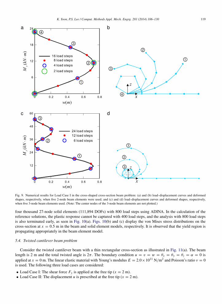
Fig. 9. Numerical results for Load Case I in the cross-shaped cross-section beam problem: (a) and (b) load–displacement curves and deformedshapes, respectively, when five 2-node beam elements were used; and (c) and (d) load–displacement curves and deformed shapes, respectively,when five 3-node beam elements used. (Note: The center nodes of the 3-node beam elements are not plotted.)

four thousand 27-node solid elements (111,894 DOFs) with 800 load steps using ADINA. In the calculation of thereference solutions, the plastic response cannot be captured with 400 load steps, and the analysis with 800 load stepsis also terminated early, as seen in Fig. 10(a). Figs. 10(b) and (c) display the von Mises stress distributions on thecross-section at x = 0.5 m in the beam and solid element models, respectively. It is observed that the yield region ispropagating appropriately in the beam element model.

5.4. Twisted cantilever beam problem

Consider the twisted cantilever beam with a thin rectangular cross-section as illustrated in Fig. 11(a). The beamlength is 2 m and the total twisted angle is 2π . The boundary condition u = v = w = θx = θy = θz = α = 0 isapplied at x = 0 m. The linear elastic material with Young’s modulus E = 2.0×1011 N/m2 and Poisson’s ratio ν = 0is used. The following three load cases are considered:

• Load Case I: The shear force Fy is applied at the free tip (x = 2 m).• Load Case II: The displacement u is prescribed at the free tip (x = 2 m).

120 K. Yoon, P.S. Lee / Comput. Methods Appl. Mech. Engrg. 281 (2014) 106–130

b

c

a

Fig. 10. Numerical results for Load Case II in the cross-shaped cross-section beam problem (five 2-node beam elements): (a) load–displacementcurves, (b) distributions of the von Mises stress obtained from the beam element model, and (c) distributions of the von Mises stress obtained fromthe solid element model.

• Load Case III: The twist angle θx is prescribed at the free tip (x = 2 m).

The twisted cantilever beam is modeled using eight 2-node beam elements, and the thin rectangular cross-section isdiscretized using one 4-node cross-sectional element, as seen in Fig. 11(b). In order to consider the twisted geometry,the director vectors are initially given as described in Fig. 11(b).

In order to obtain the reference solutions, the MITC4 shell elements (800 elements) are used in the shell elementmodel presented in Fig. 11(c). Two point loads p = 0.5Fy are applied at x = 2 m for Load Case I, and theprescribed displacement u is applied to all nodes at x = 2 m for Load Case II. All degrees of freedom are fixed atx = 0 m.

K. Yoon, P.S. Lee / Comput. Methods Appl. Mech. Engrg. 281 (2014) 106–130 121

a

bc

Fig. 11. Twisted cantilever beam problem (unit: m): (a) problem description and (b) the longitudinal and cross-sectional meshes used (8 beamelements). The twisted geometry is modeled simply through changing the director vectors of the continuum mechanics based beams (0Vk

y and0Vk

z ). (c) Shell element model (800 shell elements).

Figs. 12(a) and (b) display the load–displacement curves for Load Case I and the twist angle–stretch relation forLoad Case II. For Load Case II, Figs. 13(a) and (b) show the deformed shapes obtained from the shell element modeland beam element model, respectively. The numerical results of the beam element model exhibit good agreementwith the reference shell solutions. Note that, in order to obtain appropriate responses in this beam problem, thecoupled behavior of stretching, bending, shearing, twisting, and warping should be correctly considered in the beamformulation.

For Load Case III, Figs. 14(a) and (b) present the torsional moment Mx and longitudinal displacement u at the freetip according to the twist angle at the free tip. The corresponding deformed shapes are plotted in Fig. 14(c). As thetwist angle increases, the twisted beam is unwound from θx = 0 to 2π , and then it is rewound from θx = 2π to 4π .It is very interesting to observe the snap through phenomenon in Fig. 14(a), and the lengthening and shortening dueto the unwinding and rewinding in Fig. 14(b). Note that Load Case III cannot be analyzed using the solid and shellelement models due to convergence problems. Further studies are required for understanding the numerical difficultyas well as the physical phenomenon.

5.5. Lateral post-buckling problem

Through lateral post-buckling analyses, this section demonstrates how well the present beam element capturesthe Wagner effect. As illustrated in Fig. 15(a), a straight cantilever beam of L = 1651 mm is considered with amono-symmetric I-section, which was used in the lateral post-buckling experiment conducted by Anderson andTrahair [51]. Young’s modulus E is 65.123 × 103 N/mm2 and shear modulus G is 25.967 × 103 N/mm2.

The boundary condition u = v = w = θx = θy = θz = α = 0 is applied at x = 0 mm and the following four loadcases are considered, see Fig. 15(b):

122 K. Yoon, P.S. Lee / Comput. Methods Appl. Mech. Engrg. 281 (2014) 106–130

Fig. 12. Numerical results in the twisted cantilever beam problem: (a) load–displacement curves at the free tip for Load Case I and (b) twistangle–stretch relationship for Load Case II when the prescribed displacement is applied.

• Load Case I: The upward direction load is applied at the upper flange at the free tip.• Load Case II: The downward direction load is applied at the upper flange at the free tip.• Load Case III: The upward direction load is applied at the lower flange at the free tip.• Load Case IV: The downward direction load is applied at the lower flange at the free tip.

The loads are applied with the y-directional eccentricity of e = 0.1 mm for the consideration of imperfections.The cantilever beam is modeled using eight 2-node beam elements and the mono-symmetric I-section is discretized

using seven 16-node cubic cross-sectional elements as shown in Fig. 15(a). For each sub-beam element, 2 × 4 × 4integration is used. In order to obtain the reference solutions, the MITC4 shell elements (180 elements) are used inthe shell element model, as shown in Fig. 15(c). In order to consider the load position and eccentricity, the rigidbeam finite elements with a length of 0.1 mm are inserted at the loaded tip. All degrees of freedom are fixed atx = 0 mm.

Figs. 16(a) and (b) show the lateral post-buckling responses of the cantilever beam calculated for the four differentload cases. Different bifurcation points are observed depending on the direction and position of the load application. Topredict this interesting phenomenon accurately, it is important to include the Wagner strain in the beam formulation.Note that, in the present beam formulation, the Wagner strain is automatically considered without pre-calculatingWagner’s coefficient and the buckling modes. The bifurcation points and load–displacement curves calculated usingthe continuum mechanics based beam elements are in good agreement with the experimental results and referenceshell solutions.

For comparison, the same mesh is used for the calculations using ADINA BEAM and BEAM188. Since ADINABEAM cannot consider the load position and eccentricity, rigid beam elements are additionally used at the loadedtip to model the eccentricity. ADINA BEAM captures the complicated bifurcations with acceptable accuracy but,as mentioned, additional modeling effort is necessary. BEAM188 in ANSYS cannot capture these complicatedphenomena. Furthermore, Figs. 16(c) and (d) present the lateral post-buckling behaviors when elastoplastic materialis used (Young’s modulus E = 65.123 × 103 N/mm2, shear modulus G = 25.967 × 103 N/mm2, initial yield stressY0 = 40 N/mm2, and hardening modulus H = 0.5E).

5.6. Framed dome problem

Finally, a framed dome structure that consists of 18 beam members of a rectangular cross-section is considered asdescribed in Fig. 17 [23,52]. The boundary condition u = v = w = θx = θy = θz = α = 0 is applied at nodes on

K. Yoon, P.S. Lee / Comput. Methods Appl. Mech. Engrg. 281 (2014) 106–130 123

Fig. 13. Deformed shapes for Load Case II in the twisted cantilever beam problem: (a) shell element model and (b) beam element model.

the gray colored areas in Fig. 17. The z-directional concentrate load Fz is applied at the top of the dome. We performlarge displacement elastic and elastoplastic analyses. For the elastic analysis, Young’s modulus E = 20690 and shearmodulus G = 8830 are used. For the elastoplastic analyses, Young’s modulus E = 20690, shear modulus G = 8830,initial yield stress Y0 = 60, and hardening modulus H = 0.25E are considered. Each beam member is modeled usingfour 2-node beam elements and the rectangular cross-section is discretized using one 16-node cubic cross-sectionalelement. The 2 × 4 × 4 integration is used for each beam.

Figs. 18(a) and (b) illustrate the load–displacement curves calculated through incrementally controlling the verticaldisplacement δ with the elastic and elastoplastic materials. Fig. 18(c) shows the deformed shapes obtained from theelastic analysis. The numerical results are in good agreement with those obtained by Battini [52] and Wackerfuß andGruttmann [23].

124 K. Yoon, P.S. Lee / Comput. Methods Appl. Mech. Engrg. 281 (2014) 106–130

Fig. 14. Numerical results for Load Case III in the twisted cantilever beam problem: (a) load–displacement curve between Mx and θx at the freetip, (b) relationship between u and θx at the free tip, and (c) deformed shapes when the twist angles at the free tip are 0, π, 2π, 3π , and 4π .

6. Conclusions

In this paper, a nonlinear formulation of the continuum mechanics based beam elements was presented and theirperformance in general nonlinear analyses that focused on large twisting behaviors was demonstrated. Since the beamelements are derived from assemblages of 3D solid elements, they have inherently advanced modeling capabilitiesin the analysis of complicated 3D beam geometries including curved and twisted geometries, varying cross-sections,eccentricity, and arbitrary cross-sectional shapes [35,36]. The total Lagrangian formulation was used to obtain thecomplete tangent stiffness matrix and internal load vector with the warping displacements.

The resulting formulation can consider the fully coupled nonlinear behaviors of bending, shearing, stretching, twist-ing, and warping. In particular, large twisting and lateral buckling behaviors can be accurately predicted and, in thebeam formulation, the Wagner effect is implicitly included, unlike other beam elements. Through various numericalexamples, the strong modeling and predictive capabilities of the nonlinear formulation of the continuum mechanics

K. Yoon, P.S. Lee / Comput. Methods Appl. Mech. Engrg. 281 (2014) 106–130 125

Fig. 15. Lateral post-buckling analyses of a straight cantilever beam with a mono-symmetric I-section (unit: mm): (a) the longitudinal and cross-sectional meshes used (8 beam elements), (b) four load cases, and (c) shell element model (180 shell elements).

based beam elements were demonstrated for general nonlinear analysis. The most valuable asset of the proposed beamelements is their excellent analysis capability in large twisting problems.

Acknowledgments

This work was supported by the Basic Science Research Program through the National Research Foundation ofKorea (NRF) funded by the Ministry of Education, Science and Technology (No. 2014R1A1A1A05007219). Thiswork was also conducted under the framework of Research and Development Program of the Korea Institute ofEnergy Research (KIER) (B4-2453).

126 K. Yoon, P.S. Lee / Comput. Methods Appl. Mech. Engrg. 281 (2014) 106–130

Fig. 16. Lateral post-buckling responses for the four load cases in Fig. 15(b): (a) and (b) elastic material used, and (c) and (d) elastoplastic materialused.

Appendix. Wagner strain under pure torsion

The Wagner strain is implicitly included in the geometric nonlinear formulation of the continuum mechanics basedbeam elements. In order to verify this, the Green–Lagrange strain in the beam formulation is analytically investigated.Two configurations of a rectangular prismatic beam with free warping at time 0 and t are considered: see Fig. 19.Time 0 and t correspond to undeformed and twisted configurations, respectively. The material position vector can berewritten in the following continuum form (non-discretized form) through deduction from Eq. (1), as follows

t x =t xr + yt Vy + zt Vz +

tf t Vx , (A.1)

in which t xr is the position of the beam reference line at time t , t Vx ,t Vy , and t Vz are the director vectors, y and z

denote the position in the cross-sectional plane, and tf is the warping displacement.

K. Yoon, P.S. Lee / Comput. Methods Appl. Mech. Engrg. 281 (2014) 106–130 127

Fig. 17. Framed dome problem and the finite element discretization using the continuum mechanics based beam elements.

Fig. 18. Numerical results of the framed dome problem: (a) load–displacement curves for the elastic analysis, (b) load–displacement curve for theelastoplastic analysis, and (c) deformed shapes.

Both configurations in Fig. 17 are defined using the following vectors

0xr =t xr =

x00

, 0Vx =t Vx =

100

, 0Vy =

010

, 0Vz =

001

, t Vy =

0cos θxsin θx

,

and

t Vz =

0− sin θxcos θx

. (A.2)

128 K. Yoon, P.S. Lee / Comput. Methods Appl. Mech. Engrg. 281 (2014) 106–130

Fig. 19. Initial and deformed configurations of a prismatic straight beam.

Using Eq. (A.2) in Eq. (A.1), the material position vectors at time 0 and t are obtained

0x =

xyz

and t x =

x +tf

y cos θx − z sin θxy sin θx + z cos θx

. (A.3)

Substituting Eq. (A.3) into Eq. (23), the covariant base vectors (0g1 and t g1) are obtained

0g1 =

∂x/∂r00

and t g1 =

∂x/∂r + ∂ tf /∂r∂θx/∂r(−y sin θx − z cos θx )

∂θx/∂r(y cos θx − z sin θx )

, (A.4)

and the covariant Green–Lagrange strain t0ε11 in the configuration at time t , referred to the configuration at time 0, is

calculated

t0ε11 =

∂x

∂r

∂ tf

∂r+

12

∂ tf

∂r

2

+12(y2

+ z2)

∂θx

∂r

2

. (A.5)

Using Eq. (24), the local Green–Lagrange strain t0ε11 is given as follows:

t0ε11 =

∂ tf

∂x+

12

∂ tf

∂x

2

+12(y2

+ z2)

∂θx

∂x

2

. (A.6)

In Eq. (A.6), it is easily identified that the Green–Lagrange strain used for the continuum mechanics based beamelements automatically contains the Wagner strain term 1/2(y2

+ z2)(∂θx/∂x)2.

References

[1] K.J. Bathe, Finite Element Procedures, Prentice Hall, 1996.[2] S.P. Timoshenko, J.N. Goodier, Theory of Elasticity, McGraw Hill, 1970.[3] V.Z. Vlasov, Thin-Walled Elastic Beams, Israel Program for Scientific Translations, Jerusalem, 1961.[4] P.S. Lee, G. McClure, Elastoplastic large deformation analysis of a lattice steel tower structure and comparison with full-scale tests, J. Constr.

Steel Res. 63 (2007) 709–717.[5] A.G. Neto, C.A. Martins, P.M. Pimenta, Static analysis of offshore risers with a geometrically-exact 3D beam model subjected to unilateral

contact, Comput. Mech. 53 (2014) 125–145.[6] D.N. Kim, F. Kilchherr, H. Dietz, M. Bathe, Quantitative prediction of 3D solution shape and flexibility of nucleic acid nanostructures, Nucleic

Acids Res. 40 (2012) 2862–2868.

K. Yoon, P.S. Lee / Comput. Methods Appl. Mech. Engrg. 281 (2014) 106–130 129

[7] M. Bathe, A finite element framework for computation of protein normal modes and mechanical response, Proteins: Struct. Funct. Bioinform.70 (2008) 1595–1609.

[8] A. Kumar, S. Mukherjee, J.T. Paci, K. Chandraseker, A rod model for three dimensional deformations of single-walled carbon nanotubes, Int.J. Solids Struct. 48 (2011) 2849–2858.

[9] J. Argyris, P.C. Dunne, D.W. Scarpf, On large displacement-small strain analysis of structures with rotational degrees of freedom, Comput.Methods Appl. Mech. Engrg. 14 (1978) 401–451.

[10] J. Argyris, An excursion into large rotations, Comput. Methods Appl. Mech. Engrg. 32 (1982) 85–155.[11] K.J. Bathe, S. Bolourchi, Large displacement analysis of three-dimensional beam structures, Internat. J. Numer. Methods Engrg. 14 (1979)

961–986.[12] T. Belytschko, L.W. Glaum, Applications of higher order corotational stretch theories to nonlinear finite element analysis, Comput. Struct. 10

(1979) 175–182.[13] A. Cardona, M. Geradin, A beam finite element non-linear theory with finite rotations, Internat. J. Numer. Methods Engrg. 26 (1988)

2403–2438.[14] E.N. Dvorkin, E. Onate, J. Oliver, On a non-linear formulation for curved Timoshenko beam elements considering large displacement/rotation

increments, Internat. J. Numer. Methods Engrg. 26 (1988) 1597–1613.[15] M.A. Crisfield, A consistent co-rotational formulation for non-linear, three-dimensional, beam-elements, Comput. Methods Appl. Mech.

Engrg. 81 (1990) 131–150.[16] A. Ibrahimbegovic, On the choice of finite rotation parameters, Comput. Methods Appl. Mech. Engrg. 149 (1997) 49–71.[17] F. Gruttmann, W. Wagner, Finite element analysis of Saint–Venant torsion problem with exact integration of the elasto-plastic constitutive

equations, Comput. Methods Appl. Mech. Engrg. 190 (2001) 3831–3848.[18] A. Dutta, D.W. White, Large displacement formulation of a three-dimensional beam element with cross-sectional warping, Comput. Struct.

45 (1992) 9–24.[19] J.C. Simo, L. Vu-Quoc, A geometrically-exact rod model incorporating shear and torsion-warping deformation, Int. J. Solids Struct. 27 (1991)

371–393.[20] Y.L. Pi, N.S. Trahair, Inelastic torsion of steel I-beams, J. Struct. Eng. (ASCE) 121 (4) (1995) 609–620.[21] E. Zupan, M. Saje, D. Zupan, The quaternion-based three-dimensional beam theory, Comput. Methods Appl. Mech. Engrg. 198 (2009)

3944–3956.[22] Y.L. Pi, M.A. Bradford, B. Uy, A spatially curved-beam element with warping and Wagner effects, Internat. J. Numer. Methods Engrg. 63

(2005) 1342–1369.[23] J. Wackerfuß, F. Gruttmann, A mixed hybrid finite beam element with an interface to arbitrary three-dimensional material models, Comput.

Methods Appl. Mech. Engrg. 198 (2009) 2053–2066.[24] F. Mohri, N. Damil, M.P. Ferry, Large torsion finite element model for thin-walled beams, Comput. Struct. 86 (2008) 671–683.[25] E.J. Sapountzakis, J.A. Dourakopoulos, Lateral buckling analysis of beams of arbitrary cross section by BEM, Comput. Mech. 45 (2009)

11–21.[26] C. Basaglia, D. Camotim, N. Silvestre, Post-buckling analysis of thin-walled steel frames using generalized beam theory (GBT), Thin-Wall

Struct. 62 (2013) 229–242.[27] J. Frischkorn, S. Reese, A solid-beam finite element and non-linear constitutive modelling, Comput. Methods Appl. Mech. Engrg. 265 (2013)

195–212.[28] C. Basaglia, D. Camotim, N. Silvestre, Torsion warping transmission at thin-walled frame joints: kinematics, modelling and structural

response, J. Constr. Steel Res. 63 (2007) 709–717.[29] J. Wackerfuß, F. Gruttmann, A nonlinear Hu-Washizu variational formulation and related finite-element implementation for spatial beams

with arbitrary moderate thick cross-sections, Comput. Methods Appl. Mech. Engrg. 200 (2011) 1671–1690.[30] P.S. Lee, G. McClure, A general three-dimensional L-section beam finite element for elastoplastic large deformation analysis, Comput. Struct.

84 (2006) 215–229.[31] P.S. Lee, H.C. Noh, Inelastic buckling behavior of steel members under reversed cyclic loading, Eng. Struct. 32 (2010) 2579–2595.[32] Z.X. Li, A co-rotational formulation for 3D beam element using vectorial rotational variables, Comput. Mech. 39 (2007) 309–322.[33] M. Schulz, F.C. Filippou, Non-linear spatial Timoshenko beam element with curvature interpolation, Internat. J. Numer. Methods Engrg. 50

(2001) 761–785.[34] M. Zivkovic, M. Kojic, R. Slavkovic, N. Grujovic, A general beam finite element with deformable cross-section, Comput. Methods Appl.

Mech. Engrg. 190 (2001) 2651–2680.[35] K. Yoon, Y.G. Lee, P.S. Lee, A continuum mechanics based beam finite element with warping displacements and its modeling capabilities,

Struct. Eng. Mech. 43 (2012) 411–437.[36] K. Yoon, P.S. Lee, Modeling the warping displacements for discontinuously varying arbitrary cross-section beams, Comput. Struct. 131 (2014)

56–69.[37] M.A. Crisfield, G. Jelenic, Objectivity of strain measures in the geometrically exact three-dimensional beam theory and its finite-element

implementation, Proc. R. Soc. 455 (1999) 1125–1147.[38] A. Cardona, M. Geradin, A beam finite element non-linear theory with finite rotation, Internat. J. Numer. Methods Engrg. 26 (1988)

2403–2438.[39] A. Ibrahimbegivic, F. Frey, I. Kozar, Computational aspects of vector-like parametrization of three-dimensional finite rotations, Internat. J.

Numer. Methods Engrg. 38 (1995) 65–3673.[40] Ritto-Correa, D. Camotim, On the differentiation of the Rodrigues formula and its significance for the vector-like parameterization of

Reissner–Simo beam theory, Internat. J. Numer. Methods Engrg. 55 (2002) 1005–1032.[41] P.S. Lee, H.C. Noh, C.K. Choi, Geometry dependent MITC method for a 2-node iso-beam element, Struct. Eng. Mech. 29 (2008) 203–221.[42] K.J. Bathe, P.S. Lee, J.F. Hiller, Towards improving the MITC9 shell element, Comput. Struct. 81 (2003) 477–489.

130 K. Yoon, P.S. Lee / Comput. Methods Appl. Mech. Engrg. 281 (2014) 106–130

[43] P.S. Lee, K.J. Bathe, Development of MITC isotropic triangular shell finite elements, Comput. Struct. 82 (2004) 945–962.[44] Y.G. Lee, K. Yoon, P.S. Lee, Improving the MITC3 shell finite element by using the Hellinger–Reissner principle, Comput. Struct. 110–111

(2012) 93–106.[45] H.M. Jeon, P.S. Lee, K.J. Bathe, The MITC3 shell finite element enriched by interpolation covers, Comput. Struct. 134 (2014) 128–142.[46] E.A.S. Neto, D. Peric, D.R.J Owen, Computational Method for Plasticity: Theory and Applications, Wiley & Sons, 2008.[47] ADINA R&D, ADINA theory and modeling guide, Watertown, MA: ADINA R&D, 2013.[48] ANSYS Inc., Theory reference-Large deformation analysis, ANSYS user’s manual, 2012.[49] J.C. Simo, L. Vu-Quoc, A three-dimensional finite strain rod model. Part II: computational aspects, Comput. Methods Appl. Mech. Engrg. 58

(1986) 79–116.[50] G. Jelenic, M.A. Crisfield, Geometrically exact 3D beam theory: implementation of a strain invariant finite element for statics and dynamics,

Comput. Methods Appl. Mech. Engrg. 171 (1999) 141–171.[51] J.M. Andeson, N.S. Trahair, Stability of monosymmetric beams and cantilevers, J. Struct. Div. (ASCE) 98 (1972) 2647–2662.[52] J.M. Battini, Co-rotational Beam Elements in Instability Problems, Technical Report, Royal Institute of Technology, Stockholm, 2002.