Kumar Pakki Bharani Chandra and Da-Wei...
161
Kumar Pakki Bharani Chandra and Da-Wei Gu Nonlinear Filtering – Methods and Applications Springer
Transcript of Kumar Pakki Bharani Chandra and Da-Wei...

Kumar Pakki Bharani Chandra and Da-Wei Gu
Nonlinear Filtering – Methods and Applications
Springer


To our families


iii

Preface
This book discusses state estimation of nonlinear systems. As commonly recognised, control systems engineering and control
systems theory can be traced back to James Watt’s development of the flyball governor in the late 18th century. For a period
of some 200 years, both theory and methodology were predominantly developed in the classical frequency domain. Around
the 1960’s and in tandem with the rapid development of aerospace technology, the “state space” approach emerged as a more
accurate and more powerful tool with which to tackle control theory study and control systems design. The concept of “states”
was introduced at all in order to describe the essential properties of a control system. These system states are, however, internal
quantities of a control system; and therefore in many cases they might not may not be directly accessible, or even faithfully
measurable due to unreliability and/or high cost of sensors.
Specific techniques are therefore required to estimate the states, in order to design control schemes based on the system
states. These techniques are called “state estimators” or “filters” . The most well-known filter is the Kalman filter, which
was developed by Rudolf Kalman and others half a century ago. The Kalman filter uses the system dynamic model and real-
time input/output measurements to generate an estimation of the system states under the influence of external noises. It is an
efficient and effective estimation approach for systems subject to statistical noises. However, a limit of the Kalman filter is that
it is only applicable to linear control systems. Meanwhile, almost all control systems in the real world unfortunately display
nonlinearities, and are therefore nonlinear systems. In the real world, therefore, nonlinear state estimation becomes essential
for all practical control systems.
This book addresses the issue of state estimation for nonlinear control systems. The book starts with an introduction to
dynamic control systems and system states, as well as a brief description of the Kalman filter. In the following chapters, various
state estimation techniques for nonlinear systems are discussed. Some of the most common methods covered in relation to
nonlinear state estimation are the extended Kalman filters (EKFs). However, for an EKF design an accurate plant model and
Jacobians of the plant and measurement dynamic models are required. In the last two decades, Jacobian-free filters such as
unscented Kalman filters (UKF) and cubature Kalman filters (CKF) have been investigated to circumvent some of the inherent,
and adverse, issues of the EKF. This book will mainly focus on these Jacobian-free filters, and especially on the cubature Kalman
filter (CKF) and its extensions. Several extensions to the CKF will be derived, including cubature information filters (CIF) and
cubature H∞ filters (CH∞F). The CIF is an extension of CKF in the information domain, and it is suitable for nonlinear state
estimation with multiple sensors. For nonlinear systems with non-Gaussian noises, the CH∞F is a more effective candidate,
and is developed from CKF and H∞ filter. The square-root versions of the CIF and the CH∞F will also be further derived for
enhanced numerical stability. A number of case studies are also presented in the book to demonstrate the applicability of these
Jacobian-free filtering approaches for nonlinear systems.
This book is primarily intended for control systems researchers who are interested in nonlinear control systems. However, it
can also be readily used as a textbook for postgraduate or senior undergraduate students on nonlinear control system courses.
Lastly, practising control engineers might find this book useful in relation to the design of nonlinear control systems using
state feedback techniques. Good prerequisites for making the most of this book are a sound knowledge of classical control and
state variable control courses at undergraduate level, as well as (at least some elementary) knowledge of random signals and
stochastic processes.
The authors are grateful to many of their current and past colleagues in preparing this manuscript. The long list includes, but
is by no means limited to, Professor Ian Postlethwaite, Dr Naeem Khan, Dr Sajjad Fekriasl, Professor Christopher Edwards,
Dr Mangal Kothari, Dr Rosli Omar, Dr Rihan Ahmed, Dr Devendra Potnuru, Dr Bijnan Bandyopadhyay and Dr Ienkaran
Arasaratnam. As always, the assistance received from Springer Editors and comments from the anonymous book reviewers are
equally highly appreciated by the authors.
Leicester, U.K. Kumar Pakki Bharani Chandra
February 2018 Da-Wei Gu
v


Contents
List of algorithms . . . . . . . . . . . . . . . . . . . . . . . . . . . . . . . . . . . . . . . . . . . . . . . . . . . . . . . . . . . . . . . . . . . . . . . . . . . . . . . . . . . xi
1 Control Systems and State Estimation . . . . . . . . . . . . . . . . . . . . . . . . . . . . . . . . . . . . . . . . . . . . . . . . . . . . . . . . . . . . . . . . 1
1.1 Introductory remarks . . . . . . . . . . . . . . . . . . . . . . . . . . . . . . . . . . . . . . . . . . . . . . . . . . . . . . . . . . . . . . . . . . . . . . . . . . . . 1
1.2 Linear and nonlinear control systems . . . . . . . . . . . . . . . . . . . . . . . . . . . . . . . . . . . . . . . . . . . . . . . . . . . . . . . . . . . . . . 1
1.3 Control system design and system states . . . . . . . . . . . . . . . . . . . . . . . . . . . . . . . . . . . . . . . . . . . . . . . . . . . . . . . . . . . 3
1.4 Kalman filter and further developments . . . . . . . . . . . . . . . . . . . . . . . . . . . . . . . . . . . . . . . . . . . . . . . . . . . . . . . . . . . . 4
1.5 What is in this book . . . . . . . . . . . . . . . . . . . . . . . . . . . . . . . . . . . . . . . . . . . . . . . . . . . . . . . . . . . . . . . . . . . . . . . . . . . . 5
2 State Observation and Estimation . . . . . . . . . . . . . . . . . . . . . . . . . . . . . . . . . . . . . . . . . . . . . . . . . . . . . . . . . . . . . . . . . . . . 7
2.1 Introductory remarks . . . . . . . . . . . . . . . . . . . . . . . . . . . . . . . . . . . . . . . . . . . . . . . . . . . . . . . . . . . . . . . . . . . . . . . . . . . . 7
2.2 Mathematical preliminary . . . . . . . . . . . . . . . . . . . . . . . . . . . . . . . . . . . . . . . . . . . . . . . . . . . . . . . . . . . . . . . . . . . . . . . 8
2.3 Desired properties of state estimators . . . . . . . . . . . . . . . . . . . . . . . . . . . . . . . . . . . . . . . . . . . . . . . . . . . . . . . . . . . . . . 12
2.4 Least square estimator and Luenberger state observer . . . . . . . . . . . . . . . . . . . . . . . . . . . . . . . . . . . . . . . . . . . . . . . . 13
2.5 Luenberger state observer for a DC motor . . . . . . . . . . . . . . . . . . . . . . . . . . . . . . . . . . . . . . . . . . . . . . . . . . . . . . . . . . 15
2.6 Summary . . . . . . . . . . . . . . . . . . . . . . . . . . . . . . . . . . . . . . . . . . . . . . . . . . . . . . . . . . . . . . . . . . . . . . . . . . . . . . . . . . . . . 16
3 Kalman Filter and Linear State Estimations . . . . . . . . . . . . . . . . . . . . . . . . . . . . . . . . . . . . . . . . . . . . . . . . . . . . . . . . . . 19
3.1 Introductory remarks . . . . . . . . . . . . . . . . . . . . . . . . . . . . . . . . . . . . . . . . . . . . . . . . . . . . . . . . . . . . . . . . . . . . . . . . . . . . 19
3.2 The discrete-time Kalman filter . . . . . . . . . . . . . . . . . . . . . . . . . . . . . . . . . . . . . . . . . . . . . . . . . . . . . . . . . . . . . . . . . . . 19
3.2.1 Process and measurement models . . . . . . . . . . . . . . . . . . . . . . . . . . . . . . . . . . . . . . . . . . . . . . . . . . . . . . . . . . . 19
3.2.2 Derivation of the Kalman filter . . . . . . . . . . . . . . . . . . . . . . . . . . . . . . . . . . . . . . . . . . . . . . . . . . . . . . . . . . . . . 20
3.3 Kalman information filter . . . . . . . . . . . . . . . . . . . . . . . . . . . . . . . . . . . . . . . . . . . . . . . . . . . . . . . . . . . . . . . . . . . . . . . . 22
3.4 Discrete-timeH∞ filter . . . . . . . . . . . . . . . . . . . . . . . . . . . . . . . . . . . . . . . . . . . . . . . . . . . . . . . . . . . . . . . . . . . . . . . . . . 24
3.5 State estimation and control of a quadruple-tank system . . . . . . . . . . . . . . . . . . . . . . . . . . . . . . . . . . . . . . . . . . . . . . 26
3.5.1 Quadruple-tank system . . . . . . . . . . . . . . . . . . . . . . . . . . . . . . . . . . . . . . . . . . . . . . . . . . . . . . . . . . . . . . . . . . . 26
3.5.2 Sliding mode control of the quadruple-tank system . . . . . . . . . . . . . . . . . . . . . . . . . . . . . . . . . . . . . . . . . . . . 28
3.5.3 Combined schemes: Simulations and results . . . . . . . . . . . . . . . . . . . . . . . . . . . . . . . . . . . . . . . . . . . . . . . . . . 31
3.6 Summary . . . . . . . . . . . . . . . . . . . . . . . . . . . . . . . . . . . . . . . . . . . . . . . . . . . . . . . . . . . . . . . . . . . . . . . . . . . . . . . . . . . . . 36
4 Jacobian-based Nonlinear State Estimation . . . . . . . . . . . . . . . . . . . . . . . . . . . . . . . . . . . . . . . . . . . . . . . . . . . . . . . . . . . 41
4.1 Introductory remarks . . . . . . . . . . . . . . . . . . . . . . . . . . . . . . . . . . . . . . . . . . . . . . . . . . . . . . . . . . . . . . . . . . . . . . . . . . . . 41
4.2 Extended Kalman filter . . . . . . . . . . . . . . . . . . . . . . . . . . . . . . . . . . . . . . . . . . . . . . . . . . . . . . . . . . . . . . . . . . . . . . . . . . 41
4.3 Extended information filter . . . . . . . . . . . . . . . . . . . . . . . . . . . . . . . . . . . . . . . . . . . . . . . . . . . . . . . . . . . . . . . . . . . . . . 42
4.4 ExtendedH∞ filter . . . . . . . . . . . . . . . . . . . . . . . . . . . . . . . . . . . . . . . . . . . . . . . . . . . . . . . . . . . . . . . . . . . . . . . . . . . . . 43
4.5 A DC motor case study . . . . . . . . . . . . . . . . . . . . . . . . . . . . . . . . . . . . . . . . . . . . . . . . . . . . . . . . . . . . . . . . . . . . . . . . . . 45
4.6 Nonlinear Transformation and the effects of linearisation . . . . . . . . . . . . . . . . . . . . . . . . . . . . . . . . . . . . . . . . . . . . . 46
4.7 Summary . . . . . . . . . . . . . . . . . . . . . . . . . . . . . . . . . . . . . . . . . . . . . . . . . . . . . . . . . . . . . . . . . . . . . . . . . . . . . . . . . . . . . 50
5 Cubature Kalman Filter . . . . . . . . . . . . . . . . . . . . . . . . . . . . . . . . . . . . . . . . . . . . . . . . . . . . . . . . . . . . . . . . . . . . . . . . . . . . 53
5.1 Introductory remarks . . . . . . . . . . . . . . . . . . . . . . . . . . . . . . . . . . . . . . . . . . . . . . . . . . . . . . . . . . . . . . . . . . . . . . . . . . . . 53
5.2 CKF theory . . . . . . . . . . . . . . . . . . . . . . . . . . . . . . . . . . . . . . . . . . . . . . . . . . . . . . . . . . . . . . . . . . . . . . . . . . . . . . . . . . . 53
5.2.1 Prediction . . . . . . . . . . . . . . . . . . . . . . . . . . . . . . . . . . . . . . . . . . . . . . . . . . . . . . . . . . . . . . . . . . . . . . . . . . . . . . 53
5.2.2 Measurement update . . . . . . . . . . . . . . . . . . . . . . . . . . . . . . . . . . . . . . . . . . . . . . . . . . . . . . . . . . . . . . . . . . . . . 54
vii

5.2.3 Cubature rules . . . . . . . . . . . . . . . . . . . . . . . . . . . . . . . . . . . . . . . . . . . . . . . . . . . . . . . . . . . . . . . . . . . . . . . . . . . 54
5.3 Cubature transformation . . . . . . . . . . . . . . . . . . . . . . . . . . . . . . . . . . . . . . . . . . . . . . . . . . . . . . . . . . . . . . . . . . . . . . . . . 55
5.3.1 Polar to cartesian coordinate transformation - cubature transformation . . . . . . . . . . . . . . . . . . . . . . . . . . . . 57
5.4 Study on a brushless DC motor . . . . . . . . . . . . . . . . . . . . . . . . . . . . . . . . . . . . . . . . . . . . . . . . . . . . . . . . . . . . . . . . . . . 58
5.4.1 BLDC motor dynamics . . . . . . . . . . . . . . . . . . . . . . . . . . . . . . . . . . . . . . . . . . . . . . . . . . . . . . . . . . . . . . . . . . . 59
5.4.2 Back EMFs and PID controller . . . . . . . . . . . . . . . . . . . . . . . . . . . . . . . . . . . . . . . . . . . . . . . . . . . . . . . . . . . . . 60
5.4.3 Initialisation of the state estimators . . . . . . . . . . . . . . . . . . . . . . . . . . . . . . . . . . . . . . . . . . . . . . . . . . . . . . . . . 63
5.4.4 BLDC motor experiments . . . . . . . . . . . . . . . . . . . . . . . . . . . . . . . . . . . . . . . . . . . . . . . . . . . . . . . . . . . . . . . . . 63
5.5 Summary . . . . . . . . . . . . . . . . . . . . . . . . . . . . . . . . . . . . . . . . . . . . . . . . . . . . . . . . . . . . . . . . . . . . . . . . . . . . . . . . . . . . . 68
6 Variants of Cubature Kalman Filter . . . . . . . . . . . . . . . . . . . . . . . . . . . . . . . . . . . . . . . . . . . . . . . . . . . . . . . . . . . . . . . . . . 69
6.1 Introductory remarks . . . . . . . . . . . . . . . . . . . . . . . . . . . . . . . . . . . . . . . . . . . . . . . . . . . . . . . . . . . . . . . . . . . . . . . . . . . . 69
6.2 Cubature information filters . . . . . . . . . . . . . . . . . . . . . . . . . . . . . . . . . . . . . . . . . . . . . . . . . . . . . . . . . . . . . . . . . . . . . . 69
6.2.1 Information filters . . . . . . . . . . . . . . . . . . . . . . . . . . . . . . . . . . . . . . . . . . . . . . . . . . . . . . . . . . . . . . . . . . . . . . . . 69
6.2.2 Extended information filter . . . . . . . . . . . . . . . . . . . . . . . . . . . . . . . . . . . . . . . . . . . . . . . . . . . . . . . . . . . . . . . . 70
6.2.3 Cubature information filter . . . . . . . . . . . . . . . . . . . . . . . . . . . . . . . . . . . . . . . . . . . . . . . . . . . . . . . . . . . . . . . . 71
6.2.4 CIF in multi-sensor state estimation . . . . . . . . . . . . . . . . . . . . . . . . . . . . . . . . . . . . . . . . . . . . . . . . . . . . . . . . . 72
6.3 CubatureH∞ filters . . . . . . . . . . . . . . . . . . . . . . . . . . . . . . . . . . . . . . . . . . . . . . . . . . . . . . . . . . . . . . . . . . . . . . . . . . . . . 75
6.3.1 H∞ filters . . . . . . . . . . . . . . . . . . . . . . . . . . . . . . . . . . . . . . . . . . . . . . . . . . . . . . . . . . . . . . . . . . . . . . . . . . . . . . 75
6.3.2 ExtendedH∞ information filter . . . . . . . . . . . . . . . . . . . . . . . . . . . . . . . . . . . . . . . . . . . . . . . . . . . . . . . . . . . . 76
6.3.3 CubatureH∞ filter . . . . . . . . . . . . . . . . . . . . . . . . . . . . . . . . . . . . . . . . . . . . . . . . . . . . . . . . . . . . . . . . . . . . . . . 77
6.3.4 CubatureH∞ information filter . . . . . . . . . . . . . . . . . . . . . . . . . . . . . . . . . . . . . . . . . . . . . . . . . . . . . . . . . . . . 80
6.4 Square root version filters . . . . . . . . . . . . . . . . . . . . . . . . . . . . . . . . . . . . . . . . . . . . . . . . . . . . . . . . . . . . . . . . . . . . . . . . 83
6.4.1 Square root extended Kalman filter . . . . . . . . . . . . . . . . . . . . . . . . . . . . . . . . . . . . . . . . . . . . . . . . . . . . . . . . . 83
6.4.2 Square root extended information filter . . . . . . . . . . . . . . . . . . . . . . . . . . . . . . . . . . . . . . . . . . . . . . . . . . . . . . 85
6.4.3 Square root extendedH∞ filter . . . . . . . . . . . . . . . . . . . . . . . . . . . . . . . . . . . . . . . . . . . . . . . . . . . . . . . . . . . . . 85
6.4.4 Square root cubature Kalman Filter . . . . . . . . . . . . . . . . . . . . . . . . . . . . . . . . . . . . . . . . . . . . . . . . . . . . . . . . . 86
6.4.5 Square root cubature information filter . . . . . . . . . . . . . . . . . . . . . . . . . . . . . . . . . . . . . . . . . . . . . . . . . . . . . . 88
6.4.6 Square root cubatureH∞ filter . . . . . . . . . . . . . . . . . . . . . . . . . . . . . . . . . . . . . . . . . . . . . . . . . . . . . . . . . . . . . 90
6.4.7 Square root cubatureH∞ information filter . . . . . . . . . . . . . . . . . . . . . . . . . . . . . . . . . . . . . . . . . . . . . . . . . . . 93
6.5 State estimation of a permanent magnet synchronous motor . . . . . . . . . . . . . . . . . . . . . . . . . . . . . . . . . . . . . . . . . . . 96
6.5.1 PMSM model . . . . . . . . . . . . . . . . . . . . . . . . . . . . . . . . . . . . . . . . . . . . . . . . . . . . . . . . . . . . . . . . . . . . . . . . . . . 96
6.5.2 State estimation using SREIF and SRCIF . . . . . . . . . . . . . . . . . . . . . . . . . . . . . . . . . . . . . . . . . . . . . . . . . . . . 96
6.5.3 State estimation using SRCKF and SRCH∞F. . . . . . . . . . . . . . . . . . . . . . . . . . . . . . . . . . . . . . . . . . . . . . . . . 99
6.5.4 State estimation with multi-sensors using SREIF, SRCIF and SRCH∞IF . . . . . . . . . . . . . . . . . . . . . . . . . . 102
6.6 State estimation of a continuous stirred tank reactor (CSTR) . . . . . . . . . . . . . . . . . . . . . . . . . . . . . . . . . . . . . . . . . . . 108
6.6.1 The model . . . . . . . . . . . . . . . . . . . . . . . . . . . . . . . . . . . . . . . . . . . . . . . . . . . . . . . . . . . . . . . . . . . . . . . . . . . . . . 108
6.6.2 State estimation in the presence of non-Gaussian noises . . . . . . . . . . . . . . . . . . . . . . . . . . . . . . . . . . . . . . . . 109
6.6.3 State estimation with near-perfect measurements . . . . . . . . . . . . . . . . . . . . . . . . . . . . . . . . . . . . . . . . . . . . . . 109
6.7 Summary . . . . . . . . . . . . . . . . . . . . . . . . . . . . . . . . . . . . . . . . . . . . . . . . . . . . . . . . . . . . . . . . . . . . . . . . . . . . . . . . . . . . . 109
7 More Estimation Methods and Beyond . . . . . . . . . . . . . . . . . . . . . . . . . . . . . . . . . . . . . . . . . . . . . . . . . . . . . . . . . . . . . . . 113
7.1 Introductory remarks . . . . . . . . . . . . . . . . . . . . . . . . . . . . . . . . . . . . . . . . . . . . . . . . . . . . . . . . . . . . . . . . . . . . . . . . . . . . 113
7.2 Unscented Kalman filter . . . . . . . . . . . . . . . . . . . . . . . . . . . . . . . . . . . . . . . . . . . . . . . . . . . . . . . . . . . . . . . . . . . . . . . . . 113
7.2.1 Unscented transformation . . . . . . . . . . . . . . . . . . . . . . . . . . . . . . . . . . . . . . . . . . . . . . . . . . . . . . . . . . . . . . . . . 113
7.2.2 Unscented Kalman filter . . . . . . . . . . . . . . . . . . . . . . . . . . . . . . . . . . . . . . . . . . . . . . . . . . . . . . . . . . . . . . . . . . 115
7.3 State dependent Riccati equation (SDRE) observers . . . . . . . . . . . . . . . . . . . . . . . . . . . . . . . . . . . . . . . . . . . . . . . . . . 117
7.4 SDRE Information Filter . . . . . . . . . . . . . . . . . . . . . . . . . . . . . . . . . . . . . . . . . . . . . . . . . . . . . . . . . . . . . . . . . . . . . . . . 119
7.4.1 SDREIF in multi-sensor state estimation . . . . . . . . . . . . . . . . . . . . . . . . . . . . . . . . . . . . . . . . . . . . . . . . . . . . . 119
7.5 PMSM case revisited . . . . . . . . . . . . . . . . . . . . . . . . . . . . . . . . . . . . . . . . . . . . . . . . . . . . . . . . . . . . . . . . . . . . . . . . . . . 122
7.6 Filter robustness consideration . . . . . . . . . . . . . . . . . . . . . . . . . . . . . . . . . . . . . . . . . . . . . . . . . . . . . . . . . . . . . . . . . . . . 123
7.6.1 Uncertainties and robustness requirement . . . . . . . . . . . . . . . . . . . . . . . . . . . . . . . . . . . . . . . . . . . . . . . . . . . . 123
7.6.2 Compensation of missing sensory data . . . . . . . . . . . . . . . . . . . . . . . . . . . . . . . . . . . . . . . . . . . . . . . . . . . . . . 124
7.6.3 Selection of linear prediction coefficients and orders . . . . . . . . . . . . . . . . . . . . . . . . . . . . . . . . . . . . . . . . . . . 127
7.6.4 A case study . . . . . . . . . . . . . . . . . . . . . . . . . . . . . . . . . . . . . . . . . . . . . . . . . . . . . . . . . . . . . . . . . . . . . . . . . . . . 130
7.7 Summary . . . . . . . . . . . . . . . . . . . . . . . . . . . . . . . . . . . . . . . . . . . . . . . . . . . . . . . . . . . . . . . . . . . . . . . . . . . . . . . . . . . . . 135
viii

References . . . . . . . . . . . . . . . . . . . . . . . . . . . . . . . . . . . . . . . . . . . . . . . . . . . . . . . . . . . . . . . . . . . . . . . . . . . . . . . . . . . . . . . . . . . . . 137
Index . . . . . . . . . . . . . . . . . . . . . . . . . . . . . . . . . . . . . . . . . . . . . . . . . . . . . . . . . . . . . . . . . . . . . . . . . . . . . . . . . . . . . . . . . . . . . . . . . 143
ix


List of Algorithms
1 The Kalman filter (KF) . . . . . . . . . . . . . . . . . . . . . . . . . . . . . . . . . . . . . . . . . . . . . . . . . . . . . . . . . . . . . . . . . . . . . . . . . . . 23
2 H∞ Filter . . . . . . . . . . . . . . . . . . . . . . . . . . . . . . . . . . . . . . . . . . . . . . . . . . . . . . . . . . . . . . . . . . . . . . . . . . . . . . . . . . . . . . 25
3 Extended Kalman filter . . . . . . . . . . . . . . . . . . . . . . . . . . . . . . . . . . . . . . . . . . . . . . . . . . . . . . . . . . . . . . . . . . . . . . . . . . . 42
4 Extended Information Filter . . . . . . . . . . . . . . . . . . . . . . . . . . . . . . . . . . . . . . . . . . . . . . . . . . . . . . . . . . . . . . . . . . . . . . . 44
5 ExtendedH∞ filter . . . . . . . . . . . . . . . . . . . . . . . . . . . . . . . . . . . . . . . . . . . . . . . . . . . . . . . . . . . . . . . . . . . . . . . . . . . . . . 45
6 Cubature Kalman filter . . . . . . . . . . . . . . . . . . . . . . . . . . . . . . . . . . . . . . . . . . . . . . . . . . . . . . . . . . . . . . . . . . . . . . . . . . . 56
7 Cubature Transform . . . . . . . . . . . . . . . . . . . . . . . . . . . . . . . . . . . . . . . . . . . . . . . . . . . . . . . . . . . . . . . . . . . . . . . . . . . . . 57
8 Cubature information filter . . . . . . . . . . . . . . . . . . . . . . . . . . . . . . . . . . . . . . . . . . . . . . . . . . . . . . . . . . . . . . . . . . . . . . . . 74
9 CubatureH∞ filter . . . . . . . . . . . . . . . . . . . . . . . . . . . . . . . . . . . . . . . . . . . . . . . . . . . . . . . . . . . . . . . . . . . . . . . . . . . . . . 79
10 CubatureH∞ information filter . . . . . . . . . . . . . . . . . . . . . . . . . . . . . . . . . . . . . . . . . . . . . . . . . . . . . . . . . . . . . . . . . . . . 82
11 Square root extended Kalman filter . . . . . . . . . . . . . . . . . . . . . . . . . . . . . . . . . . . . . . . . . . . . . . . . . . . . . . . . . . . . . . . . . 84
12 Square root cubature information filter . . . . . . . . . . . . . . . . . . . . . . . . . . . . . . . . . . . . . . . . . . . . . . . . . . . . . . . . . . . . . . 89
13 Square root cubatureH∞ filter . . . . . . . . . . . . . . . . . . . . . . . . . . . . . . . . . . . . . . . . . . . . . . . . . . . . . . . . . . . . . . . . . . . . 92
14 Square root cubatureH∞ information filter . . . . . . . . . . . . . . . . . . . . . . . . . . . . . . . . . . . . . . . . . . . . . . . . . . . . . . . . . . 95
15 Unscented Transform . . . . . . . . . . . . . . . . . . . . . . . . . . . . . . . . . . . . . . . . . . . . . . . . . . . . . . . . . . . . . . . . . . . . . . . . . . . . 114
16 Unscented Kalman Filter . . . . . . . . . . . . . . . . . . . . . . . . . . . . . . . . . . . . . . . . . . . . . . . . . . . . . . . . . . . . . . . . . . . . . . . . . 117
17 State Dependent Riccati Equation Information Filter (SDREIF) . . . . . . . . . . . . . . . . . . . . . . . . . . . . . . . . . . . . . . . . . 121
18 Selection of the LP filter order (first method) . . . . . . . . . . . . . . . . . . . . . . . . . . . . . . . . . . . . . . . . . . . . . . . . . . . . . . . . . 130
19 Selection of the LP filter order (second method) . . . . . . . . . . . . . . . . . . . . . . . . . . . . . . . . . . . . . . . . . . . . . . . . . . . . . . 130
xi


List of Tables
1.1 Key differences between Wiener and Kalman filters [4]. . . . . . . . . . . . . . . . . . . . . . . . . . . . . . . . . . . . . . . . . . . . . . . . 4
3.1 Quadruple-tank parameters. . . . . . . . . . . . . . . . . . . . . . . . . . . . . . . . . . . . . . . . . . . . . . . . . . . . . . . . . . . . . . . . . . . . . . . . 27
5.1 Back EMFs as functions of θ and ω . . . . . . . . . . . . . . . . . . . . . . . . . . . . . . . . . . . . . . . . . . . . . . . . . . . . . . . . . . . . . . . . 60
5.2 The functions fab, fbc and fca . . . . . . . . . . . . . . . . . . . . . . . . . . . . . . . . . . . . . . . . . . . . . . . . . . . . . . . . . . . . . . . . . . . . . 61
5.3 Switching functions for hysteresis current control . . . . . . . . . . . . . . . . . . . . . . . . . . . . . . . . . . . . . . . . . . . . . . . . . . . . . 61
xiii


List of Figures
1.1 A box furnace heating plant . . . . . . . . . . . . . . . . . . . . . . . . . . . . . . . . . . . . . . . . . . . . . . . . . . . . . . . . . . . . . . . . . . . . . . . 2
1.2 An example of a combined state estimation - control approach. . . . . . . . . . . . . . . . . . . . . . . . . . . . . . . . . . . . . . . . . . 3
1.3 Flow-chart of the book. . . . . . . . . . . . . . . . . . . . . . . . . . . . . . . . . . . . . . . . . . . . . . . . . . . . . . . . . . . . . . . . . . . . . . . . . . . . 5
2.1 Open Loop Block Diagram . . . . . . . . . . . . . . . . . . . . . . . . . . . . . . . . . . . . . . . . . . . . . . . . . . . . . . . . . . . . . . . . . . . . . . . 7
2.2 Normal probability density function. . . . . . . . . . . . . . . . . . . . . . . . . . . . . . . . . . . . . . . . . . . . . . . . . . . . . . . . . . . . . . . . 11
2.3 Luenberger (full-order) state observer. . . . . . . . . . . . . . . . . . . . . . . . . . . . . . . . . . . . . . . . . . . . . . . . . . . . . . . . . . . . . . . 15
2.4 States of Luneberger observer for dc motor . . . . . . . . . . . . . . . . . . . . . . . . . . . . . . . . . . . . . . . . . . . . . . . . . . . . . . . . . . 16
2.5 Luneberger observer estimation error for dc motor . . . . . . . . . . . . . . . . . . . . . . . . . . . . . . . . . . . . . . . . . . . . . . . . . . . . 16
3.1 A combined SMC-H∞ filter approach. . . . . . . . . . . . . . . . . . . . . . . . . . . . . . . . . . . . . . . . . . . . . . . . . . . . . . . . . . . . . . . 26
3.2 Quadruple-Tank System [51]. . . . . . . . . . . . . . . . . . . . . . . . . . . . . . . . . . . . . . . . . . . . . . . . . . . . . . . . . . . . . . . . . . . . . . 27
3.3 Proposed scheme using SMC andH∞ filter for quadruple-tank system . . . . . . . . . . . . . . . . . . . . . . . . . . . . . . . . . . . 32
3.4 Actual and estimated states of the quadruple-tank using the Kalman filter in the presence of Gaussian noises. . . 33
3.5 Actual and estimated states of the quadruple-tank usingH∞ filter in the presence of Gaussian noises. . . . . . . . . . 34
3.6 Estimation errors for the quadruple-tank using Kalman andH∞ filters in the presence of Gaussian noises. . . . . . 35
3.7 RMSEs using Kalman andH∞ filters in the presence of non-Gaussian noises. . . . . . . . . . . . . . . . . . . . . . . . . . . . . . 36
3.8 Actual and estimated states of the quadruple-tank using the Kalman filter in the presence of non-Gaussian noises. 37
3.9 Actual and estimated states of the quadruple-tank usingH∞ filter in the presence of non-Gaussian noises. . . . . . 38
3.10 Estimation errors for the quadruple-tank using Kalman andH∞ filters in the presence of non-Gaussian noises. . 39
3.11 RMSEs using Kalman andH∞ filters in the presence of non-Gaussian noises. . . . . . . . . . . . . . . . . . . . . . . . . . . . . . 40
4.1 Actual and estimated velocity using EKF . . . . . . . . . . . . . . . . . . . . . . . . . . . . . . . . . . . . . . . . . . . . . . . . . . . . . . . . . . . . 46
4.2 Estimation error of EKF . . . . . . . . . . . . . . . . . . . . . . . . . . . . . . . . . . . . . . . . . . . . . . . . . . . . . . . . . . . . . . . . . . . . . . . . . . 46
4.3 Actual and estimated velocity using EH∞F . . . . . . . . . . . . . . . . . . . . . . . . . . . . . . . . . . . . . . . . . . . . . . . . . . . . . . . . . . 47
4.4 Estimation error using EH∞F . . . . . . . . . . . . . . . . . . . . . . . . . . . . . . . . . . . . . . . . . . . . . . . . . . . . . . . . . . . . . . . . . . . . . 47
4.5 2000 random points (∗) are generated with range and bearings, which are uniformly distributed between ±0.02
and ±20. . . . . . . . . . . . . . . . . . . . . . . . . . . . . . . . . . . . . . . . . . . . . . . . . . . . . . . . . . . . . . . . . . . . . . . . . . . . . . . . . . . . . . 49
4.6 2000 random measurements are generated with range and bearings, which are uniformly distributed between
±0.02 and ±20. These random points are then processed through the nonlinear polar to cartesian coordinate
transformation and are shown as ∗. The true mean and the uncertainty ellipse are represented by • and solid
line, respectively. . . . . . . . . . . . . . . . . . . . . . . . . . . . . . . . . . . . . . . . . . . . . . . . . . . . . . . . . . . . . . . . . . . . . . . . . . . . . . . . . 49
4.7 2000 random measurements are generated with range and bearings, which are uniformly distributed between
±0.02 and ±20. These random points are then processed through the nonlinear polar to cartesian coordinate
transformation and are shown as ∗. The true mean and the linearised mean are represented by • and , and true
and linearised uncertainty ellipses are represented by solid and dotted lines, respectively. . . . . . . . . . . . . . . . . . . . 50
5.1 2000 random measurements are generated with range and bearings, which are uniformly distributed between
±0.02 and ±20. These random points are then processed through the nonlinear polar to cartesian coordinate
transformation and are shown as ∗. The true-, linearised-, and cubature transformation means are represented
by •, , and ⋆, respectively. True, linearised, and cubature transformation uncertainty ellipses are represented
by solid, dotted, dashed-dotted and dashed lines, respectively. . . . . . . . . . . . . . . . . . . . . . . . . . . . . . . . . . . . . . . . . . . 58
5.2 Block diagram of full state feedback BLDC motor. . . . . . . . . . . . . . . . . . . . . . . . . . . . . . . . . . . . . . . . . . . . . . . . . . . . 59
5.3 Proposed scheme for a BLDC motor. . . . . . . . . . . . . . . . . . . . . . . . . . . . . . . . . . . . . . . . . . . . . . . . . . . . . . . . . . . . . . . . 62
xv

5.4 Experimental setup for BLDC drive . . . . . . . . . . . . . . . . . . . . . . . . . . . . . . . . . . . . . . . . . . . . . . . . . . . . . . . . . . . . . . . . 64
5.5 Block diagram for BLDC drive experiment. . . . . . . . . . . . . . . . . . . . . . . . . . . . . . . . . . . . . . . . . . . . . . . . . . . . . . . . . . 64
5.6 Speed controller scheme using CKF. . . . . . . . . . . . . . . . . . . . . . . . . . . . . . . . . . . . . . . . . . . . . . . . . . . . . . . . . . . . . . . . . 64
5.7 Experimental results for low reference speed (30 rpm). . . . . . . . . . . . . . . . . . . . . . . . . . . . . . . . . . . . . . . . . . . . . . . . . 65
5.8 Experimental results for high reference speed (2000 rpm). . . . . . . . . . . . . . . . . . . . . . . . . . . . . . . . . . . . . . . . . . . . . . 66
5.9 Experimental results with load variations. . . . . . . . . . . . . . . . . . . . . . . . . . . . . . . . . . . . . . . . . . . . . . . . . . . . . . . . . . . . 67
5.10 Experimental results with stator resistance variations. . . . . . . . . . . . . . . . . . . . . . . . . . . . . . . . . . . . . . . . . . . . . . . . . . 67
5.11 Estimation errors with de-tuned stator inductance. . . . . . . . . . . . . . . . . . . . . . . . . . . . . . . . . . . . . . . . . . . . . . . . . . . . . 68
6.1 Actual and estimated states of PMSM using SREIF and SRCIF. . . . . . . . . . . . . . . . . . . . . . . . . . . . . . . . . . . . . . . . . . 97
6.2 RMSE of PMSM using SREIF and SRCIF. . . . . . . . . . . . . . . . . . . . . . . . . . . . . . . . . . . . . . . . . . . . . . . . . . . . . . . . . . . 97
6.3 Actual and estimated states using decentralised SREIF and SRCIF. . . . . . . . . . . . . . . . . . . . . . . . . . . . . . . . . . . . . . . 98
6.4 RMSE of PMSM using decentralised SREIF and SRCIF. . . . . . . . . . . . . . . . . . . . . . . . . . . . . . . . . . . . . . . . . . . . . . . 99
6.5 Actual and estimated states of PMSM for non-Gaussian noise using SRCKF and SRCH∞F. . . . . . . . . . . . . . . . . . 100
6.6 RMSEs of the PMSM using SRCKF and SRCH∞F. . . . . . . . . . . . . . . . . . . . . . . . . . . . . . . . . . . . . . . . . . . . . . . . . . . 100
6.7 RMSEs of x3 with near-perfect measurements for the PMSM using SRCKF and SRCH∞F. . . . . . . . . . . . . . . . . . 101
6.8 PMSM states using decentralised SREH∞IF and decentralised SRCH∞IF for low Gaussian noise. . . . . . . . . . . . 103
6.9 RMSE of PMSM speed using decentralised SREH∞IF and decentralised SRCH∞IF for low Gaussian noise. . . . 103
6.10 PMSM states using decentralised SREH∞IF and decentralised SRCH∞IF for high Gaussian noise. . . . . . . . . . . . 104
6.11 RMSE of PMSM speed using decentralised SREH∞IF and decentralised SRCH∞IF for high Gaussian noise. . . 104
6.12 PMSM states using decentralised SREH∞IF and decentralised SRCH∞IF for low non-Gaussian noise. . . . . . . . 105
6.13 RMSE of PMSM speed using decentralised SREH∞IF and decentralised SRCH∞IF for low non-Gaussian noise.105
6.14 PMSM states using decentralised SREH∞IF and decentralised SRCH∞IF for high non-Gaussian noise. . . . . . . . 106
6.15 RMSE of PMSM speed using decentralised SREH∞IF and decentralised SRCH∞IF for high non-Gaussian
noise. . . . . . . . . . . . . . . . . . . . . . . . . . . . . . . . . . . . . . . . . . . . . . . . . . . . . . . . . . . . . . . . . . . . . . . . . . . . . . . . . . . . . . . . . . 106
6.16 PMSM simulation results in the presence of near-perfect Gaussian and non-Gaussian noise in multi-sensor
SRCH∞IF. . . . . . . . . . . . . . . . . . . . . . . . . . . . . . . . . . . . . . . . . . . . . . . . . . . . . . . . . . . . . . . . . . . . . . . . . . . . . . . . . . . . . . 107
6.17 Actual and estimated states of CSTR for non-Gaussian noise using SRCKF and SRCH∞F. . . . . . . . . . . . . . . . . . . 110
6.18 CSTR’s RMSEs of x1 in the presence of non-Gaussian noise using SRCKF and SRCH∞F. . . . . . . . . . . . . . . . . . . 110
6.19 CSTR’s RMSEs of x1 in the presence of near-perfect measurement using SRCKF and SRCH∞F. . . . . . . . . . . . . 111
7.1 2000 random measurements are generated with range and bearings, which are uniformly distributed between
±0.02 and ±20. These random points are then processed through the nonlinear polar to cartesian coordinate
transformation and are shown as ∗. The true, linearised and unscented transformation means are represented
by •, and , respectively. True, linearised and unscented transformation uncertainty ellipses are represented
by solid, dotted and dashed-dotted lines, respectively. . . . . . . . . . . . . . . . . . . . . . . . . . . . . . . . . . . . . . . . . . . . . . . . . . 116
7.2 Actual and measured data. . . . . . . . . . . . . . . . . . . . . . . . . . . . . . . . . . . . . . . . . . . . . . . . . . . . . . . . . . . . . . . . . . . . . . . . . 123
7.3 State estimation using single- and multi-sensor SDREIF. . . . . . . . . . . . . . . . . . . . . . . . . . . . . . . . . . . . . . . . . . . . . . . . 124
7.4 Error plots using single- and multi-sensor SDREIF. . . . . . . . . . . . . . . . . . . . . . . . . . . . . . . . . . . . . . . . . . . . . . . . . . . . 125
7.5 MSD two cart system. . . . . . . . . . . . . . . . . . . . . . . . . . . . . . . . . . . . . . . . . . . . . . . . . . . . . . . . . . . . . . . . . . . . . . . . . . . . . 131
7.6 Performance of KF without measurement loss. . . . . . . . . . . . . . . . . . . . . . . . . . . . . . . . . . . . . . . . . . . . . . . . . . . . . . . . . . . . . . 132
7.7 KF without measurement loss for states x1, x3 and x4. . . . . . . . . . . . . . . . . . . . . . . . . . . . . . . . . . . . . . . . . . . . . . . . . . . . . . . . . 133
7.8 Estimation of state x2. . . . . . . . . . . . . . . . . . . . . . . . . . . . . . . . . . . . . . . . . . . . . . . . . . . . . . . . . . . . . . . . . . . . . . . . . . . . . . . 133
7.9 Estimation analysis of states x1, x3 and x4. . . . . . . . . . . . . . . . . . . . . . . . . . . . . . . . . . . . . . . . . . . . . . . . . . . . . . . . . . . . . . . . . 134
7.10 Estimation error of state x2. . . . . . . . . . . . . . . . . . . . . . . . . . . . . . . . . . . . . . . . . . . . . . . . . . . . . . . . . . . . . . . . . . . . . . . . . . . 134
7.11 Estimation error of states x1, x3 and x4. . . . . . . . . . . . . . . . . . . . . . . . . . . . . . . . . . . . . . . . . . . . . . . . . . . . . . . . . . . . . . . . . . . 135
7.12 Kalman filter gains of ZeroGKF approach . . . . . . . . . . . . . . . . . . . . . . . . . . . . . . . . . . . . . . . . . . . . . . . . . . . . . . . . . . . . . . . . 136
7.13 Kalman filter gains of ComKF approach . . . . . . . . . . . . . . . . . . . . . . . . . . . . . . . . . . . . . . . . . . . . . . . . . . . . . . . . . . . . . . . . . 136
xvi
Chapter 1
Control Systems and State Estimation
1.1 Introductory remarks
This book is about state estimation of control systems, nonlinear control systems in particular. Control systems are dynamic
systems and exist in engineering, physical sciences as well as in social sciences. The earliest, somehow commonly recognised
control system could be traced back to James Watt’s flyball governor in 1769. The study on control systems, analysis and system
design, has been continuously developed ever since. Until the mid of last century the control systems under investigation had
been single-input-single-output (SISO), time-invariant systems and were mainly deterministic and of lumped-parameters. The
approaches used were of frequency-domain nature, so called classical approaches. In classical control approaches, control
system’s dynamic behaviour is represented by transfer functions. Rapid developments and needs in aerospace engineering in
the 1950s and 1960s greatly drove the development of control system theory and design methodology, particularly in the state-
space approach that is powerful towards multi-input-multi-output (MIMO) systems. State-space models are used to describe the
dynamic changes of the control system. In the state-space approach, the system states determine how the system is dynamically
evolving. Therefore, by knowing the system states one can know the system’s properties and by changing the trajectory of
system states successfully with specifically designed controllers one can achieve the objectives for a certain control system.
However, the states of a control system are “internal”parameters and are not always accessible. Figure 1.1 below is a sketch
diagram of a box furnace heating plant. Parts to be heated are placed within the furnace and heated by the gas and air (the input)
pumped in from one end of the furnace. The control objective is to control the temperature and the heating time of the part by
adjustment of the input. In this system, the temperature within the furnace is the state variable. Strictly speaking this plant is
a distributive control system. By partitioning, however, it can be represented by lumped-parameter model satisfactorily. Even
so, it is difficult to measure the temperature of the part in the furnace due to the high temperature which requires expensive
thermocouple (sensor) of top quality. That may not be a solution the Industry would accept. State estimation methods are
necessary in such a scenario.
Another major reason for the need of state estimation is due to the existence of noises and plant uncertainties. Industrial
control systems are always operating in real environments and are inevitably affected by random noises and/or disturbances. On
the other hand, the mathematical representation of the system dynamics, namely, the system model, is difficult to be derived fully
and accurately, due to the complexity of the plant and cost in modelling and controller design/operation. The initial condition
of the operation of the control system is usually unknown. Even if a system model is accurate initially, the model parameters
would vary due to tear-and-wear. Hence, the idea of using the model and input to work out the system states is impractical. State
estimation methods are indeed needed in practice. In the following sections of this chapter, more control system properties will
be introduced and the use of state estimation is to be further justified.
1.2 Linear and nonlinear control systems
A control system or plant or process is an interconnection of components to perform certain tasks and to yield a desired
response, i.e. to generate desired signals (the output), when it is driven by manipulating (a group of) signals (the input). In this
book, a control system is a causal, dynamic system, i.e. the output depends on not only the present input but also the input
applied at the previous time.
Due to the increasing complexity of physical systems to be controlled and rising demands on system properties, most in-
dustrial control systems are no longer single-input and single-output (SISO) but multi-input and multi-output (MIMO) systems
with a high interrelationship (coupling) between these channels. The number of (state) variables in a system could be very large
as well. These systems are called multivariable systems.
1

.
T1
T2
T3
T4
T5
T6
Gas/Air
Fig. 1.1: A box furnace heating plant
In order to analyse and design a control system, it is advantageous if a mathematical representation of such a relationship
(namely, a model) is available. The system dynamics is usually governed by a set of differential equations, either ordinary
differential equations, for lumped-parameter systems which are the systems this book considers, or partial differential equations
for distributive systems.
By introducing a set of appropriate state variables, the dynamic behaviour of a time-invariant, control system may be repre-
sented by the following mathematical equations (the model), in the continuous-time case:
x(t) = f(x(t),u(t))+w(t)
z(t) = h(x(t),u(t))+v(t) (1.1)
where x(t) ∈Rn is the state vector, u(t) ∈Rm the input (control) vector, and z(t) ∈Rp the output (measurement) vector; and w(t)
and v(t) are process noise and measurement noise, respectively.
In the discrete-time case, the model is as
xk = f(xk−1,uk−1)+wk−1 (1.2)
zk = h(xk,uk)+vk (1.3)
where k is the time index.
The noises w and v are assumed to be zero mean Gaussian-distributed, random variables with covariances of Qk−1 and Rk.
The continuous-time and discrete-time models listed above are generic. They may represent just the plant dynamics in the
open-loop system scenario or the dynamics of both the plant and controller in the closed-loop system scenario.
In this book, control systems are mainly considered in their discrete-time form.
Control systems can be classified as linear systems or nonlinear systems. A control system is linearif the functions f and h
in (1.1) and (1.1) satisfy the superposition rules with regard to the state x, the input u as well as the initial state x(0).
In the linear case , the system model can be described as
x(t) = Ax(t)+Bu(t)+w(t)
y(t) = Cx(t)+Du(t)+v(t) (1.4)
In the case of discrete-time systems, similarly the model is given by
xk = Fk−1xk−1+Gk−1uk−1 +wk−1, (1.5)
zk = Hkxk+vk, (1.6)
2

1.3 Control system design and system states
Control systems design is necessary for almost all practical systems. The task of a control engineer is to design a controller
to stabilise an unstable system and/or to achieve the desired performance in the presence of uncertainties, including dynamic
perturbations (parametric variations and unmodelled dynamics), and disturbance and noises. In general, there are two categories
of control systems, the open-loop and closed-loop control systems [43]. Open-loop systems are “simple” in structure and less
costly. In an open-loop control system, the output has no effect on the control action. For a given input, the system gives a
certain output, if in an uncertainty-free scenario. In the presence of dynamic perturbations, the stability of open-loop systems is
not guaranteed, even if the originally built, nominal system is stable. Similarly, the tracking performance would be affected by
the disturbance in an open-loop structure. In open-loop systems, no measurements are made at the output for control purpose
and hence it does not have the feedback mechanism. In contrast to an open-loop system, a closed-loop control system uses
sensors/transducers to measure the actual output to adjust the input in order to achieve desired output. The measure of the
output in this use is called the feedback signal, and a closed-loop system is also called a feedback system. In a closed-loop
system, the feedback signals are compared with the reference signals, which possibly produces errors in most cases. Based on
these error signals, the controller generates the inputs to the system which help the outputs to reach their desirable values.
Any dynamical system can be characterised by a set of state variables. If the state variables are used to obtain the control
signals, it is called as a state feedback control system and if the controller is directly based on the measured outputs, then it is
called as output feedback systems. In most of the real-world applications it is not always possible to access the complete state
information due to the limitations on sensors and/or cost consideration, such as in the box furnace heating system introduced
earlier. If some of the sensors are very noisy or expensive or physically unsuitable for the control system, then it is not advisable
to use them to measure the states either. Rather, one can use the state estimation methods to obtain or, more accurately, to
estimate the unavailable states using the input and output information together with known dynamic structure of the system.
Control systems can be classified in several ways like: linear and nonlinear, deterministic and stochastic, time-varying and
time-invariant, lumped parameter and distributive parameter systems, etc. Control schemes for these systems can be designed
based on the output or state information. State feedback controllers include pole placement control, linear quadratic regulator
(LQR), dynamic inversion control, etc. and output feedback controllers include proportional-integral-derivative (PID) control,
linear quadratic Gaussian control, etc. Many controllers can be designed based on either state feedback or output feedback
like sliding mode control, H∞ control, model predictive control, etc. One would also note that even if the complete state
information is not available, the state feedback controllers could still be designed using estimated states obtained from state
estimation methods. A combined state estimation-control approach is shown in Figure 1.2. If the state estimator in Figure 1.2
is the Kalman filter, then this approach may lead to a linear quadratic Gaussian (LQG) controller. A similar kind of approach is
to be explored later in the book using a sliding mode control and anH∞ filter on a quadruple tank system. The use of Kalman
filter andH∞ filter will be compared via simulations.
Fig. 1.2: An example of a combined state estimation - control approach.
State estimation is a process of estimating the unmeasured states using the noisy outputs, control inputs along with process
and measurement models. It has been an active research area for several decades. Similar to control systems, state estimation can
also be classified as linear and nonlinear, deterministic and stochastic, etc. The earliest state estimation problem was considered
in the field of astronomical studies by Karl Friedrich Gauss in 1795, where the planet and comet motion was studied using the
telescopic measurements [107]. Gauss used the least square method as the estimation tool. After more than 140 years of Gauss’
invention, Andrey Nikolaevich Kolmogorov [67] and Norbert Wiener [120] solved the linear least-square estimation problem
for stochastic systems. Kolmogorov studied discrete least-estimation problems, whereas, Wiener studied the continuous-time
problems [56]. Wiener filter1 is also a useful tool in signal processing and communication theory. But when it specifically comes
to the state estimation, Wiener filter is seldom used as it only deals with the stationary processes. Rudolf Emil Kalman extended
Wiener’s work for more generic non-stationary processes in the path breaking paper [58]. The Wiener filter was developed in
3

the frequency domain and is mainly used for signal estimation, whereas, the Kalman filter was developed in the time domain
for state estimation. Key differences between Wiener and Kalman filters can be given in Table 1.1.
Wiener filter Kalman filter
Mainly used for signal estimation. Can be used for signal and state estimation.
Signal and process noises are stationary. A generalisation of Wiener filter for non-stationary signals.
Can be obtained by spectral factorisation methods. Requires matrix Riccati equation solutions.
Basically, a frequency domain approach. A time domain (state space) approach.
Table 1.1: Key differences between Wiener and Kalman filters [4].
As the main emphasis of this book is on the state estimation, the Wiener filter will not be further discussed.
1.4 Kalman filter and further developments
The Kalman filter can be defined as “an estimator used to estimate the state of a linear dynamic system perturbed by Gaussian
white noise using measurements that are linear functions of the system state but corrupted by additive Gaussian white noise”
[38]. The Kalman filter and its variants are the main estimation tools for practical systems in the past several decades. The
Kalman filter can be represented in an alternative form as the information filter, where the parameters of interest are the
information states and the inverse of covariance matrix rather than the states and covariance matrix. Information filters are
more flexible in initialisation compared to conventional Kalman filters and the update stage is computationally economic, and
it can be readily extended for multi-sensor fusion; for more details please see [4], [83], and will be discussed further later in
the book. Both Kalman and information filters can be derived in the Gaussian framework and they need accurate process and
measurement models.
The early success of the Kalman filter in 1960s in aerospace applications was due to the availability of accurate system
models, which were obtained after spending millions of dollars on the space programmes [104]. However, it is not worth to
spend that huge amount of money in most other industrial applications in order to get an accurate model. One of the alternatives
to the Kalman filter is to develop the estimator using the concepts of robust control. Several researchers have explored the robust
control theory, specially the H∞ theory, to develop robust state estimators [41], [84], [122], [98], [12], [7]. In H∞ filters, the
requirements on the accurate models or ‘apriori’ statistical noise properties can be relaxed to a certain extent.
In real-time implementation of Kalman filters, the propagated error covariance matrices may become ill-conditioned, which
may eventually hinder the filtering operation. This can happen if some of the states are measured with greater precision than
others, where the elements of covariance matrix corresponding to accurately measured states will have lower values, while the
other entries will have higher values. These types of ill-conditioned covariance matrices may cause numerical instability during
the online implementation. To circumvent these difficulties, one can use square-root Kalman filters, where the square root of
the error covariance matrices are propagated. Key properties of the square-root filters include symmetric positive definiteness
of error covariances, availability of square-root factors, doubled order precision, improved numerical accuracy, etc. [57], [59],
[81], [118], [17], which are useful in the filter implementation and applications. Similar to square-root Kalman filters, the
information and H∞ filters can also be explored as square-root information filters [13], [91], [88] and square-root H∞ filters
[57], [44].
Initially the Kalman filter was developed for linear systems. However, most of the real-world problems are nonlinear and
hence the Kalman filter has been further extended for nonlinear systems. Stanley F. Schmidt was the first researcher to explore
the Kalman filter for nonlinear systems, while doing so he developed the so called extended Kalman filter (EKF), see [78]
for fascinating historical facts about the development of the EKF for practical applications. However, EKFs are only suitable
for “mild” nonlinearities where the first-order approximations of the nonlinear functions are available and EKFs also require
evaluation of state Jacobians at every iterations. To overcome some of the limitations of EKF, an unscented Kalman filter (UKF)
has been proposed [54], [53], which is a derivative free filter. The UKF uses the deterministic sampling approach to capture the
mean and covariances with sigma points and in general has been shown to perform better than EKF in nonlinear state estimation
problems. The UKF has been further explored in the information domain for decentralised estimation [117], [16], [72]. There
are a few other nonlinear estimation techniques found in the literature, to name a few, Rao-Blackwellised particle filters [31],
1 In general, the term “filter” is frequently used for state estimators in the estimation literature. This is due to Wiener, who studied the continuous-time
estimation problem and noted that his algorithm can be implemented using a linear circuit. In circuit theory, the filters are used to separate the signals
over different frequency ranges. Wiener’s solution extended the classical theory of filter design to problems of obtaining the filtered signals from noisy
measurements [57].
4

which are the improved version of particle filters [6], Gaussian filters [49], state dependent Riccati equation filters [82], [85],
sliding mode observers [121], Fourier-Hermite Kalman filter [96], etc.
Recently, the cubature Kalman filter (CKF) [5] has been proposed for nonlinear state estimation. CKF is a Gaussian approx-
imation of Bayesian filter, but provides a more accurate filtering estimate than existing Gaussian filters. In this book, the CKF
will be further explored for multi-sensor state estimation and for non-Gaussian noises. The efficacy of the proposed methods
are demonstrated on various simulation examples.
1.5 What is in this book
A brief introduction can be found in the first two chapters on control systems, system states and state estimation. In addition, a
DC motor is used to illustrate the usage of the classical Luenberger state observer in Chapter 2. This book will then introduce
and discuss several important state estimation approaches together with application of these approaches in a few case studies.
A graphical representation of the book is shown in Figure 1.3.
Fig. 1.3: Flow-chart of the book.
Before discussions on state estimation for nonlinear control systems that is the main theme of the book, Chapter 3 introduces
the linear estimation techniques first. It begins with mathematical preliminaries of Kalman filter, information filter andH∞ filter.
The detailed derivation of Kalman filter and the game theory approach to the discrete H∞ filter is briefly discussed. Towards
the end of this chapter, a combined use of the sliding mode control (SMC) and an H∞ filter for a quadruple-tank system is to
be proposed. It is assumed that, out of the system’s four states only two states are directly accessible. The complete state vector
is estimated using anH∞ filter and the SMC is designed based on the estimated states. The proposedH∞ filter based SMC can
be easily extended for other practical systems.
5

From Chapter 4 the book concentrates on nonlinear state estimation techniques. Chapter 4 presents several Jacobian-based
nonlinear state estimation approaches, including the extended Kalman filter (EKF), extended information filter (EIF) and ex-
tendedH∞ filter (EH∞F). These approaches all have a linear case origin and are corresponding extensions for nonlinear control
system state estimations.
Chapter 5 focusses on the cubature Kalman filter (CKF), the idea behind this approach and its derivation based on cubature
transformation. CKF is a Gaussian approximation of Baysian filtering, but provides a more accurate estimation than other
existing Gaussian filters.
Chapter 6 presents variants of cubature Kalman filters, including the cubature information filter (CIF), the cubature H∞filter (CH∞F) and the cubature H∞ information filter (CH∞IF). CIF is the fusion of extended H∞ filter and CKF. It can be
easily extended to multi-sensor state estimation, where the data from various nonlinear sensors are fused. The CH∞F is derived
for state estimation of nonlinear systems with general noises; not limited to Gaussian noises. For numerical accuracy, the
square root versions of introduced nonlinear filtering approaches introduced so far are presented. Among that, the square root
cubature information filter (SRCIF) is developed using the J-unitary transformation for the single sensor as well as multi-sensor
cases. The efficacy of the multi-sensor square root CIF is validated in a permanent magnet synchronous motor example and a
continuous stirred tank reactor problem, in the presence of Gaussian and non-Gaussian noises.
Chapter 7, the last chapter of the book, mainly discusses other nonlinear state estimation methods, the unscented Kalman
filter (UKF) and the state-dependent Riccati equation (SDRE) observer. Chapter 7, and the book, ends at considering an impor-
tant topic, the so-called “robustness” property of linear and nonlinear state estimators, which is a topic for current and future
research. The considerations include inaccurate knowledge on noises and missing of measurement data. These commonly oc-
cur in real world environment and are thus crucial for successful industrial applications of control systems state estimation
approaches.
A number of application examples, including a quadruple-tank system, coordinate transformations that forms the base of
simultaneous localisation and mapping (SLAM) cases study, a permanent magnet synchronous motor, a highly nonlinear and
high fidelity brush-less DC motor and a continuously stirred tank reactor case, are frequently used to illustrate and to compare
the use of various methods introduced in the book.
6

Chapter 2
State Observation and Estimation
2.1 Introductory remarks
Basically, the term “Filtering” is referred to a technique to extract information (signal in this context) from noise contaminated
observations (measurements). If the signal and noise spectra are essentially non-overlapping, the design of a frequency-domain
filter that allows the desired signal to pass while attenuating the unwanted noise would be a possibility. A classical filter could
be either low pass, band pass/stop or high pass. However, when the noise and information signals are overlapped in spectrum,
then the design of a filter to completely separate the two signals would not be possible. In such a situation the information has
to be retrieved through estimation, smoothing or prediction. Figure 2.1 below shows a general diagram of an open-loop system
(plant) subject to noise contamination at the output end.
perturbations
noises
input output measurementSystem (Plant)
u(t)x(t)
y(t) z(t)
∆
n(t)
Fig. 2.1: Open Loop Block Diagram
With regard to Figure 2.1, filtering usually means to retrieve the (output) signal y(t) from the noise contaminated data
(measurement) z(t) at time t, using the measurement up to the current time t [120]. Smoothing, on the other hand, indicates
to recover information of y(t) with the help of measurements obtained later than at time t, i.e. z(t+ τ) for some τ > 0. It can
be called a delay in producing the information of y(t) as compared to the filtering operation. Another important concept is
prediction, defined as the forecasting of information processing. In prediction, the information of y(t + τ) for some τ > 0 is
forecasted based on the measurement up to time t.
In the context of a control system as it being the subject of this book, the retrieval of the system state is more involved.
Generally speaking, the system state is “internal” information and therefore is not directly accessible in many cases. What
makes it even worse is that the system would suffer from uncertainties including dynamic perturbations, disturbances and
noises. To estimate the state of a control system, it is vital to employ all available information including the system input (u(t)),
the measurement (z(t)) which could be contaminated, and the system model which is usually inaccurate/incomplete though.
State estimation has long been an active research topic in the control system engineering because of its importance in analysis
of system behaviour as well as in design of control schemes such as state feedback controllers.
7

In this chapter, following the introduction of a few mathematical terms in the next section, a summary of desired properties
of state estimation algorithms (estimators) one would expect will be presented. The chapter finishes with the simplest approach
of state estimation, namely “state observation” for linear, time-invariant (LTI), deterministic systems, together with a DC motor
case to illustrate its usage.
2.2 Mathematical preliminary
It is useful to include in the book some basic definitions related to random variables and their statistical properties such as mean,
variance, correlation and distribution of random processes. The descriptions of those are quite concise. Interested readers may
find details in standard textbooks on probability and stochastic systems like [26, 76, 87].
Random variable
In Probability Theory, a random variable is a variable whose value varies randomly, within a usually known range and
subject to “chances” . The possible values of a random variable might represent the possible outcomes of a yet-to-be-performed
experiment. A random variable (or a random signal) cannot be characterised by a simple, well-defined mathematical function
and its future values cannot be precisely predicted. However, the probability and statistical properties (e.g. mean and variance)
can be used to analyse the behavior of a random variable. If an event ε is a possible outcome of a random experiment then
the probability of this event can be denoted by p(ε) and generally all possible outcomes of the random experiment, if finite,
represented by ε j , ∀ j = 1,2, ...n, follow
0 ≤ p(ε) ≤ 1 and
n∑
j=1
p(ε j) = 1 (2.1)
The probability density function of a continuous random variable X, is a function which is summed to obtain the probability
that the variable takes a value x in a given interval. It is defined as
f (x) =dF(x)
dx(2.2)
where F(x) is the cumulative distribution function1 .
The probability density function satisfies
F(∞) =
∫ ∞
−∞f (x)dx = 1 (2.4)
Similarly, for a discrete random variable, its probability distribution (or probability function) is a list of probabilities associ-
ated with each of its possible value, i.e.
p(xi) = P[X = xi] (2.5)
The probability distribution satisfies the criteria defined in (2.1).
Mean
The expected or mean value of a random variable indicates the average or “central” value of that random variable. The mean
value gives a general idea about a random variable instead of the complete details of its probability distribution (of a discrete
random variable) or the probability density function (of a continuous random variable). Two random variables with different
distributions (or density functions) might have the same mean values, hence the mean value itself does not reveal the complete
information of a random variable. If X is a continuous random variable with probability density function f (x), the expected or
1 The cumulative distribution function gives the probability that the random variable X satisfies
F(x) = p(X < x) ∀−∞ < x <∞ (2.3)
.
8
mean value can be represented as
µ = E[X] :=
∫ ∞
−∞x f (x)dx (2.6)
Similarly, if X is a discrete random variable with possible values xi, where i = 1,2,3...,n and its probability p(xi) is given
as P(X = xi), then the mean or expected value can be defined as
µ = E[X] :=∑
xiP(X = xi) (2.7)
where the elements are summed over all possible values of the random variable X.
Variance
The variance of a random variable shows how widely the values of that random variable are likely to be. The larger the
variance, the more scattered the observations about its mean value. In other words, variance shows the concentration of the
random variable’s distribution with regard to its mean value. Variance of a continuous random variable X, denoted by σ2 or
V(x), is defined by
σ2 = V(x) :=
∫ ∞
−∞(x−E(x))2 f (x)dx (2.8)
The square root of the variance of a random variable is known as standard deviation (σ).
If the random variable X is discrete, then its variance Var[X] is defined as
Var[X] = E[(X−µ)2]
= E[X2−2µX+µ2]
= E[X2]−2µE[X]+µ2
= E[X2]−µ2
= E[X2]−E[X]2. (2.9)
The variance and standard deviation of a random variable are always non-negative.
Covariance, correlation and correlation coefficient
The covariance of two random variables X and Y shows how much X and Y change together. If these two random variables
change values in the same direction, i.e. when X takes greater (or lesser) values the random variable Y takes greater (lesser)
values, too, then the covariance of X and Y is positive. When the opposite scenario occurs, the covariance would be negative.
The sign of the covariance shows the tendency in the linear relationship between X and Y.
The covariance Cov(X,Y) of X and Y is defined as
Cov(X,Y) = E[(X−E[X])(Y−E[Y])]
= E[XY −XE[Y]−E[X]Y+E[X]E[Y]]
= E[XY]−E[X]E[Y]−E[X]E[Y]+E[X]E[Y]
= E[XY]−E[X]E[Y]. (2.10)
In statistics, correlation shows how strongly (or, weakly) two or more variables are related to each other. Linear correlation
(also known as Pearson’s correlation) determines the extent to which two variables are linearly related (or proportional) to each
other.
Correlation coefficient denoted by ρ is a number. It indicates the degree to which two variables X and Y are linearly related.
Let the mean and the standard deviation of X (Y) be denoted by µX (µY ) and σX (σY ), respectively. The correlation coefficient
of X and Y, ρX,Y , can be expressed as
9

ρX,Y =Cov(X,Y)
σXσY
=E[(X−µX)(Y −µY)]
σXσY
=E[(X−E(X))(Y−E(Y))]√E(X2)−E2(X)
√E(Y2)−E2(Y)
=E(XY)−E(X)E(Y)√
E(X2)−E2(X)√E(Y2)−E2(Y)
. (2.11)
If the two variables are independent then ρX,Y = 0 and if one variable (say Y ) is a linear function of the other variable (X),
then ρX,Y is either 1 or −1. What should be noted is that the correlation (or correlation coefficient) measures linear relationship
only. It is possible that there exists a strong nonlinear relationship between two variables while ρX,Y = 0. In the case of nonlinear
relationship between two random variables, the correlation coefficient does not show the influence of one variable on the other.
Autocorrelation
A random variable X could be a process of the time. At each time instant, X(t) (or, Xt) itself is a random variable. Such
X(·) can be called a random process. More will be described shortly below. The term “autocorrelation” is the correlation of
a signal process with itself [89]. It indicates the similarity between observations as a function of the time separation. In other
words, autocorrelation of a random process describes the correlation between the values of the same process at different points
in time. It is also sometimes called as lagged or serial correlation. Therefore, if X is a process with the mean µ and the standard
deviation σ, both are functions of the time, then the autocorrelation of X, γ(t,m) with regard to two different time instants t and
m can be defined as
γ(t,m) :=E[(Xt−µt)(Xm−µm)]
σtσm
(2.12)
If the variance of this random process over the time is non-zero finite, then γ(t,m) is well defined and takes value between
1 and −1. If Xt is a second order stationary process (sometimes called wide-sense stationary (WSS) process), i.e. the mean
and variance are time independent, then its autocorrelation only depends on the time-lapse between the pair of time instants.
Therefore, if let τ := t−m, (2.12) can be re-written as
γ(τ) =E[(Xt−µ)(Xt+τ−µ)]
σ2(2.13)
Autocorrelation helps in finding repeating patterns, such as periodic changes or fundamental frequency of a signal which
cannot be determined due to some unwanted factors like noise. A positive autocorrelation value indicates some sort of tendency
for a system to remain in the same status from one time instant to another. For example, the likelihood of tomorrow being rainy
is higher if today is raining than if today is dry [23].
Normal distribution
The “normal distribution” (also known as Gaussian distribution) is a very important class of statistical distribution. This type
of distribution is symmetric about the mean value of the random variable and has a bell-shaped density curve with a single
peak. Any normal distribution can be fully specified by two quantities: the mean µ (or m), where the peak of the density lies at,
and the standard deviation σ, which indicates the spreading distribution. In other words, if a real-valued random variable X is
normally distributed with mean m and variance σ2, where σ ≥ 0, then it can be written as
X ∼ ℵ(m,σ2) (2.14)
i.e. the random variable X is normally distributed with mean m and variance σ2. The normal probability density function of a
scalar value can be shown analytically to be
f (x) =1
σ√
2πe
[− (x−m)2
2σ2]
(2.15)
10

The integral of the above function (which corresponds to the area under the curve) is unity. Sketch of a typical normal
distribution is shown in Figure 2.2 for σ = 4 and m = 13.
−40 −30 −20 −10 0 10 20 30 400
0.01
0.02
0.03
0.04
0.05
0.06
0.07
0.08
0.09
0.1
X
f(X
)
Fig. 2.2: Normal probability density function.
The probability that a normal distributed function lies outside ±2σ is approximately 0.05. Standard normal distribution is
defined with mean m = 0 and standard deviation σ = 1. Therefore, from Equation (2.15), a standard normal distribution can be
written as
f (x) =1√2π
e[− x2
2] (2.16)
The normal distribution (2.15) can be extended to the cases of two and more random variables. For the case of two random
variables, the bivariate normal distribution is as below:
f (x1, x2) =1
σ1σ2
√1−ρ2
e
[−
x21
σ21
−2ρx1x2σ1σ2
+x22
σ22
2(1−ρ2)
]
(2.17)
where ρ is the correlation function between the two random variables x1 and x2. Similarly, for the case of n random variables,
the multivariate normal distribution function is
f (x1, x2, · · · , xn) =1
(2π)n/2‖P‖1/2 e[− (x−m)T P−1(x−m)
2σ2]
(2.18)
where the vector xT := [x1, x2, · · · , xn]; and, the vector m := E[x] and the matrix P := E[(x−m)(x−m)T ] are the mean and
covariance of the vector x, respectively.
Random process
A random or stochastic process is a process whose behaviour is not completely predictable. A random process can, however,
be characterised by its statistical properties. Due to randomness of random variables, the average values from a collection of
signals rather than from one individual signal, are usually investigated. Therefore, a random process X(t), t ∈ T is a family
of random variables where the index set T might be discrete (T = 0,1,2, · · · ) or continuous (T = (0,∞)). For a discrete time
system, the word random sequence is the preferred terminology to use instead of random process. A daily life example of
random processes could be the hourly rainfall at a certain place, for instance.
Stationary process
“Stationarity” is the quality in which statistical properties of a process do not change with time [116]. In other words, the
probability density function (continuous case) or the probability distribution (discrete case) of a stationary random variable X(t)
11

is independent of time t. Wherever the distribution is seen for some segment, the dynamics remain the same. This means that it
does not matter when in time one observes the process.
Definition 1:
A process Xt, t ∈ ℜ is said to be a weak-sense stationary (WSS) process if
1. E[X2t ] <∞, ∀t ∈ ℜ ,
2. E[Xt] = µt = µ, and
3. Cov(Xt, Xm) = E[(Xt −µt)(Xm−µm)] = σ2(t,m) = σ2(t−m), ∀t,m ∈ ℜ.
In other words one can say that a weak-sense stationary process must have finite variance, constant mean (first moment) and
the second moment should only depend on (t−m) and not on t or m [113].
Definition 2:
A process Xt, t ∈ℜ is strictly stationary process if all its finite (cumulative) distribution function is independent of the time
shift, i.e. for any finite number n and ∀t1, t2, · · · , tn ∈ ℜ, ∀h ∈ ℜ,
p(Xt1 ≤ x1, Xt2 ≤ x2, · · · ,Xtn ≤ xn) = F(xt, xt2 , · · · , xtn )
= F(xt1+h, xt2+h, · · · , xtn+h)
= p(Xt1+h ≤ x1,Xt2+h ≤ x2, · · · ,Xtn+h ≤ xn) (2.19)
Most statistical prediction methods are based on the assumption that the time series can be considered approximately sta-
tionary.
White noise
White noise is a random signal (or process) in which the power spectrum is distributed uniformly over all the frequency
components in the full infinite range. This is purely a theoretical concept because if a signal has the same power at all com-
ponents frequency, this is equivalent to a signal whose total power is infinite and therefore it is impossible to generate such a
signal in the real world. However in practice, for a finite frequency range, a “white” signal with a flat spectrum can be assumed.
Mathematically, a random signal (or, a vector signal) v is a white signal if and only if it possesses the following two
properties:
mv := E[v] = 0
Rv := E[vvT ] = σ2I (2.20)
A continuous white noise process w holds the same properties as:
mw(t) := E[w(t)] = 0
Qw(t1 ,t2) := E[w(t1)w(t2)T ] =1
2S δ(t1− t2) (2.21)
i.e. it has zero mean everywhere and infinite power at zero time shift.
2.3 Desired properties of state estimators
Obviously, the purpose of using a state estimator is to obtain an estimate of the system states. That is to produce an x(t) such
that it reflects the true value (information) of the actual state x(t). This property would usually be referred as “convergence” : the
estimate x(t) needs to converge to the actual state x(t) or in almost all state estimation cases involving stochastic signals (noises),
as in this book, the expectation of the magnitude of the difference between x(t) and x(t) should be zero. For a vector state, it
turns out to be E[‖x(t)− x(t)‖2
]= 0, in terms of so-called the mean square error (MSE). However, in the context of filtering,
this property is more often called stability. It indicates that the convergence property comes from the asymptotic stability of the
dynamic system governing the estimation error e(t) = x(t)− x(t). Such use of this terminology could trace back to the classical
12

state observer like the Luenberger observer discussed in the next section. With the term of stability, the concept of convergence
rate can also be linked to various stability definitions, such as exponential stability.
Many state estimation algorithms consist of, like most approaches discussed in this book, two phases in operation: predict
and update. In the prediction phase, the states and covariance functions are predicted based on the (known) system dynamics,
i.e. the state evolution functions in a state space model as well as on the estimated states, the covariances at the previous time
instant, and the system input information at the current time. In the updating phase, with the newly obtained measurements, the
state estimates and covariance are updated. In reality, system dynamics may not be known exactly nor be truly incorporated
in the system model. Also, the statistic properties of the noises involved in the system running such as their covariances may
not be known exactly. These would seriously influence the effectiveness of state estimation algorithms. Thus, how well a state
estimation algorithm can deal with system dynamics and noises variations is important and worth considering. This property
is usually referred to as sensitivity. It is part of a broader property called robustness. The robustness consideration may also
include the scenario of measurement missing, for instance, that will be discussed later in this book.
Applicability and computational efficiency are among other features requested for a state estimation algorithm. For example,
the case of non-Gaussian noises needs to be considered in a practical application; and, approaches such as the square root form
of algorithms may be preferable in solving a real world problem for numerical stability. Interested readers will find a great
amount of discussions on these features in the literature [3, 15, 62–64].
2.4 Least square estimator and Luenberger state observer
Often, when data (or, measurements) are corrupted by some unwanted (noise) signal, the information contained in the data will
have to be obtained by the means of filtering (estimation). In the context of control systems, to get the information of the state is
the process of state estimation. In a wider sense, this is also a process of determination of system “parameters” from available
data. Hence, it may also be called “parameter estimation” . A well-known optimal parameter estimator is next introduced in
this section which bears the minimum prediction (or estimation) error, and is called “least square estimator” (LSE). Before the
introduction of LSE, linear control system models will be presented below first.
Linear control system models
It is a fact that almost all control systems in the real world would have certain nonlinearities, in the form of inherent nonlinear
dynamics, input saturation or others. However, it is also true that many nonlinear systems can be approximated by linear system
models, though locally in most cases. Obviously it is much more convenient and easier to analyse a linear system and to conduct
control scheme design for a linear system. Analysis tools and synthesis approaches for linear control systems are also much
more mature. Of course, one has to bear in mind in the process of analysis and design around a linear model the nonlinear
nature of the underlying control system, if the actual system is nonlinear which is the usual case.
For linear, finite-dimensional, time-invariant, continuous-time control systems, a state space model is of the form
x(t) = Ax(t)+Bu(t)
y(t) = Cx(t)+Du(t)
where A, B, C and D are constant matrices with appropriate dimensions.
Equation (2.22) is called the state equation and (2.22) the output equation. The state equation is a set of linear, ordinary
differential equations with constant coefficients; the output y(t) is a memoryless function of x(t) and u(t). In many systems,
D = 0.
Least square estimation
Linear least square estimation is an estimation method for unknown parameters in a linear regression model with the aim
of minimising the sum of the square of differences between the true parameters and the estimated parameters. Consider an
unknown parameter vector x that is related to the data or observation vector z in the following equation:
z = Hx+v (2.22)
This could be be the case of the output equation (2.22) with D = 0 of the linear, time-invariant system model introduced
earlier. One may assume that the measuring process of the system output is contaminated by a noise v, that is a common
13
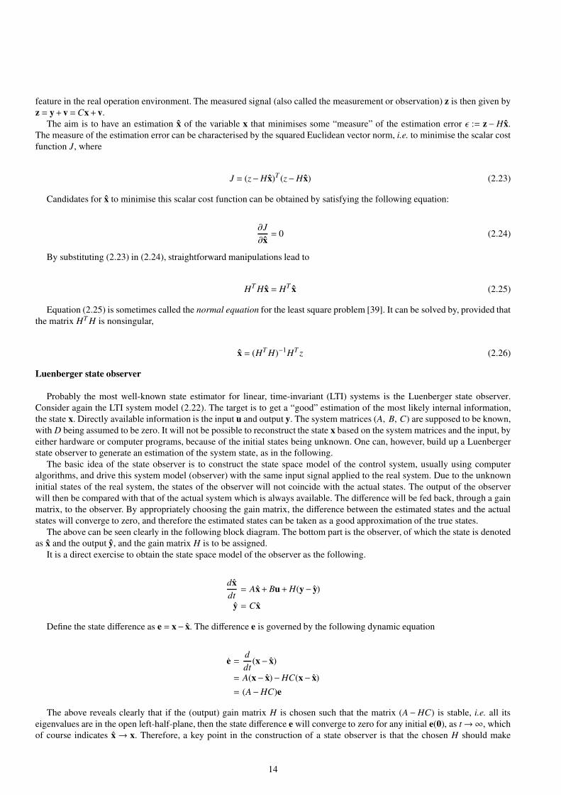
feature in the real operation environment. The measured signal (also called the measurement or observation) z is then given by
z = y+v =Cx+v.
The aim is to have an estimation x of the variable x that minimises some “measure” of the estimation error ǫ := z−Hx.
The measure of the estimation error can be characterised by the squared Euclidean vector norm, i.e. to minimise the scalar cost
function J, where
J = (z−Hx)T (z−Hx) (2.23)
Candidates for x to minimise this scalar cost function can be obtained by satisfying the following equation:
∂J
∂x= 0 (2.24)
By substituting (2.23) in (2.24), straightforward manipulations lead to
HT Hx = HT x (2.25)
Equation (2.25) is sometimes called the normal equation for the least square problem [39]. It can be solved by, provided that
the matrix HT H is nonsingular,
x = (HT H)−1HT z (2.26)
Luenberger state observer
Probably the most well-known state estimator for linear, time-invariant (LTI) systems is the Luenberger state observer.
Consider again the LTI system model (2.22). The target is to get a “good” estimation of the most likely internal information,
the state x. Directly available information is the input u and output y. The system matrices (A, B, C) are supposed to be known,
with D being assumed to be zero. It will not be possible to reconstruct the state x based on the system matrices and the input, by
either hardware or computer programs, because of the initial states being unknown. One can, however, build up a Luenberger
state observer to generate an estimation of the system state, as in the following.
The basic idea of the state observer is to construct the state space model of the control system, usually using computer
algorithms, and drive this system model (observer) with the same input signal applied to the real system. Due to the unknown
initial states of the real system, the states of the observer will not coincide with the actual states. The output of the observer
will then be compared with that of the actual system which is always available. The difference will be fed back, through a gain
matrix, to the observer. By appropriately choosing the gain matrix, the difference between the estimated states and the actual
states will converge to zero, and therefore the estimated states can be taken as a good approximation of the true states.
The above can be seen clearly in the following block diagram. The bottom part is the observer, of which the state is denoted
as x and the output y, and the gain matrix H is to be assigned.
It is a direct exercise to obtain the state space model of the observer as the following.
dx
dt= Ax+Bu+H(y− y)
y = Cx
Define the state difference as e = x− x. The difference e is governed by the following dynamic equation
e =d
dt(x− x)
= A(x− x)−HC(x− x)
= (A−HC)e
The above reveals clearly that if the (output) gain matrix H is chosen such that the matrix (A−HC) is stable, i.e. all its
eigenvalues are in the open left-half-plane, then the state difference e will converge to zero for any initial e(0), as t→∞, which
of course indicates x→ x. Therefore, a key point in the construction of a state observer is that the chosen H should make
14

♥
♥
u
B
+
+
x ∫ x
C
A
y
+
−
ey
H
B
++
+
A
∫˙x x
C y
x
Fig. 2.3: Luenberger (full-order) state observer.
(A−HC) stable. A question remains: what kind of system would assure the existence of such H? The next theorem answers it
and its proof can be readily found in most control course textbooks that cover the state space approach.
Theorem 2-1: The eigenvalues of (A−HC) can be arbitrarily assigned if and only if the matrix pair (A, C) is completely ob-
servable.
Luenberger state observer introduced above is for the continuous-time systems. Similar development exists for discrete-time
systems, too.
2.5 Luenberger state observer for a DC motor
Consider a second order DC motor (linearised) model with the current and angular velocity as its states, x = [i ω]T and the
current as the output [79],
i = −Ri+KT iω−V
L(2.27)
ω = KT Li2 −Dmω (2.28)
where, R = 7.2Ω, L = 0.5H, Dm = 0.0004, J = 0.00071 and KT = 0.01. By linearising the above model, the state space matrices
can be obtained as:
A =
−R+KTω0
L− KT
Li02KT i0
J−Dm
J
B =
[1L
0
]
C =[1 0
]
D = 0
The operating points are i0 = 0.1A and ω0 = 1rad/s. The reference velocity and the output velocity are compared and the
error is sent to a PID controller with Kp = 8.8, Ki = 267.9 and Kd = 0.03. The output of the designed PID controller is taken
15

as the input to the DC motor. However, it is assumed that only the current of the DC motor is measured and the velocity is
estimated using a Luneberger observer. The Luenberger observer gain, H, is designed such that the eigenvalues of (A−HC) are
placed at −1 and −20, respectively. The corresponding Luenberger gain for the DC motor is obtained as H = [6 −4240.39]T
and is then used in (2.27) to estimate the angular velocity. Instead of the actual velocity, the estimated velocity from Luenberger
observer is compared with the reference velocity to generate the error which is then given to the PID controller. Fig. 2.4 shows
the reference velocity, actual velocity and the velocity obtained by using the Luenberger observer. The actual and estimated
velocity are very close to each other; the error between them is shown in Fig. 2.5.
0 2 4 6 8 100
1
2
3
4
5
6
Time (sec)
Speed (
rpm
)
Reference speed
Actual speed
Estimated speed using Luenberger
Fig. 2.4: States of Luneberger observer for dc motor
0 2 4 6 8 100
0.2
0.4
0.6
0.8
1
1.2
1.4
1.6
1.8x 10
−3
Time (sec)
Lu
en
be
rge
r sp
ee
d e
rro
r (r
pm
)
Fig. 2.5: Luneberger observer estimation error for dc motor
The above simulations shows how well the estimated signal is close to the actual signal. It also shows of course the successful
design of the PID controller which makes the output of the DC motor closely follow the reference signal. In this example, the
nonlinearity of the DC motor is relatively “mild”The linearised model is thus “close” to the nonlinear model at the chosen
operating point (also called the equilibrium point) and the Luenberger observer therefore works well in such cases. Readers
may notice as well that no noises are supposed to affect the running of the motor. Interested readers may play with the observer
gain and/or the PID controller parameter values to see the efficiency of the observer and of the controller designated, too.
2.6 Summary
This is a preliminary chapter. It introduced some mathematical components which are necessary for the development of state
estimation approaches to be discussed in the rest of the book. It also introduced the basic ideas of state estimators, their usage
16

and their importance in control systems analysis and control schemes design. This chapter also introduced the classical state
estimator, Luenberger state observer, with a DC motor example. Luenberger state observer is widely used in re-construction of
states for a linear and time-invariant control system which is deterministic and is supposed to be free from noise contamination.
Luenberger state observer and the application example offered a taste for the simplest case of system states estimation.
17


Chapter 3
Kalman Filter and Linear State Estimations
3.1 Introductory remarks
As discussed in the earlier chapters, the system state contains vital information for control system analysis and design, but it
is not always directly measurable. Control engineers will have to obtain the information of system states based on accessible
information of the known system dynamics, inputs and outputs (measurements). What makes this task more complicated is that
industrial control systems are always operating in an environment with uncertainties. Uncertainties include dynamic perturba-
tions and unwanted, as well as unknown, external signals such as noises. Noises affect the operation of sensors and transducers,
and thus generate inaccurate measurements. That would give wrong information about the states of the control system and even
possibly lead to failure of a control scheme in a feedback system structure. To retrieve the actual, true information from noise-
contaminated signals is the target of the filtering (estimation) process. The study on state estimation has been an active research
subject for several decades and always plays a key role in practical applications. Real-life applications of the state estimation
include state and parameter estimation in chemical process plants, electrical machinery, data assimilation, econometrics, fault
detection and isolation, control system design, etc., where either sensors are noisy or it is difficult to measure the states due to
various physical settings. Linear state estimation deals with the state estimation of linear systems and linear measurement mod-
els. Although, all the practical systems have nonlinearities involved as discussed earlier and nonlinear system state estimation
is the major theme of this book, it is worth to explore some linear state estimation methods as a basis for nonlinear estimation
approaches. In this chapter, the epic development, the Kalman filter (KF) , will be introduced followed by the information
filter and theH∞ filters. Similar to the previous chapter, and the following chapters as well, applications of these filters will be
demonstrated at a later part of the chapter. One may see [19] for more details.
3.2 The discrete-time Kalman filter
In early 1940s Kolmogorov and Wiener discussed the problem of linear least square estimation for a stochastic process [56,
57, 67, 120]. Kolmogorov formulated the filter design problem using statistical and frequency-domain characteristics. However
their results are based on stationary processes with infinite or semi-infinite observation intervals. R.E. Kalman presented the
design of now well-known Kalman filter (KF) in [58]. Kalman filtering approach is an on-line, recursive method adopted to
estimate the state of a system with noise-contaminated observations. Kalman filter is to be introduced in this section next.
The signals involved in an industrial control system (such as input, output and state) are most likely continuous-time signals.
However, due to the wide use of digital computers nowadays in control engineering and due to the recursive (iterative) nature
of most estimation schemes, control systems, and consequently the state estimators, considered in this book will be modelled
and discussed in the discrete-time context.
3.2.1 Process and measurement models
Consider the discrete linear process and measurement models as
xk = Fk−1xk−1 +Gk−1uk−1 +wk−1, (3.1)
zk = Hkxk +vk, (3.2)
19

where k ≥ 1 is the time index, xk is the state vector, uk the control input, zk the measurement (output), wk−1 and vk are the
process and measurement noises, respectively.
Noises are random signals. A control system with stochastic components can be called a stochastic system. Strictly speaking
though, the dynamics of a stochastic system should be a stochastic processes. The control systems considered in this book are
mainly those with deterministic dynamics but influenced by stochastic signals namely noises.
The process and measurement noises are assumed to be Gaussian-distributed1 random variables, which have zero means and
covariances of Qk−1 and Rk, respectively,
wk−1 =N(0,Qk−1)
vk =N(0,Rk)
whereN represents the Gaussian or normal probability distribution.
The process and measurement noises at any time are assumed to be independent of the system state
E [wixTj ] = 0, E [wiw
Tj ] =Qiδi j ∀ i, j
and
E [vixTj ] = 0, E [viv
Tj ] = Riδi j ∀ i, j
where δi j is the Dirac function and E [·] is the expectation operator.
3.2.2 Derivation of the Kalman filter
The derivation in this section closely follows the one given in [29] and [33]. The Kalman filter gives an estimate, xi| j, that
minimises the mean-squared estimation error conditioned on the measurements sequence, Z j = [z1,z2, . . . ,z j]. The estimated
state is the expected value of the state conditioned on the measurements sequence and is given by
xi| j = E[xi|Z j]. (3.3)
The error between the actual and estimated states is defined by
xe,i| j = xi− xi| j (3.4)
and the covariance of xi| jPi| j = E[xe,i| jx
Te,i| j|Z j]. (3.5)
The Kalman filter is a recursive algorithm consisting of two stages: the time update (also known as a priori or prediction)
stage, and the measurement update (a posteriori estimate or filtering update) stage. In the prediction stage, the state and the
covariance at the kth instant are predicted based on the information available at the (k−1)th instant. Once the (new) measurement
is obtained at the kth instant, the predicted state and covariance are then “modified” to yield the updated state estimate and
updated covariance at the kth instant. The whole process repeats itself recursively.
The predicted state can be obtained by taking the expectation of the state model conditioned on measurements up to the
(k−1)th instant and is given by
xk|k−1 = E[xk |Zk−1]
= E[(Fk−1xk−1 +Gk−1uk−1 +wk−1)|Zk−1]
= Fk−1E[xk−1 |Zk−1]+Gk−1uk−1 +E[wk−1|Zk−1]
= Fk−1xk−1|k−1 +Gk−1uk−1. (3.6)
Similarly, the predicted covariance at the kth instant based on the (k−1)th can be found as
1 The Kalman’s original derivation did not use the Bayes’ rule and does not require the exploitation of any specific error distribution information.
The Kalman filter is the minimum variance estimator if the noise is Gaussian, and it is the linear minimum variance estimator for linear systems with
non-Gaussian noises [54, 58, 104, 115].
20

Pk|k−1 = E[(xe,k|k−1xTe,k|k−1)|Zk−1]
= E[(xk − xk|k−1)(xk − xk|k−1)T |Zk−1]
= E[(Fk−1xk−1 −Fk−1xk−1|k−1 +wk−1)(Fk−1xk−1 −Fk−1xk−1|k−1 +wk−1)T |Zk−1]
= Fk−1E[(xk−1 − xk−1|k−1)(xk−1 − xk−1|k−1)T |Zk−1]FTk−1 +E[(wk−1wT
k−1)|Zk−1]
= Fk−1Pk−1|k−1FTk−1 +Qk−1. (3.7)
The predicted measurement and the innovation vector, which is the difference between actual measurement and the predicted
measurement, can be obtained as
zk|k−1 = E[zk |Zk−1]
= E[Hkxk +vk|Zk−1
]
= Hk(E[xk|Zk−1]+E[vk|Zk−1]
= Hkxk|k−1 (3.8)
and
νk = zk − zk|k−1
= zk −Hkxk|k−1. (3.9)
After obtaining the predicted state and covariance, the next task is to obtain the updated state and covariance for the recursive
process. The updated state vector can be calculated from the predicted state and the innovation vector and is given as
xk|k = xk|k−1 +Kkνk (3.10)
where, Kk is the Kalman gain, which dictates the influence of the innovation on the updated state vector. The error between the
actual and updated states is given by
xe,k|k = xk − xk|k= xk − [xk|k−1 +Kkνk]
= xe,k|k−1 −Kkνk
= xe,k|k−1 −Kk(zk −Hkxk|k−1)
= xe,k|k−1 −Kk(Hkxk +vk −Hkxk|k−1)
= xe,k|k−1 −Kk(Hkxe,k|k−1 +vk)
= (I−KkHk)xe,k|k−1 −Kkvk (3.11)
where, I is the identity matrix of an appropriate size.
The covariance update can be written as
Pk|k = E[(xk − xk|k)(xk − xk|k)T |Zk]
= E[xe,k|kxTe,k|k |Zk]
= E[(I−KkHk)xe,k|k−1 −Kkvk(I−KkHk)xe,k|k−1 −KkvkT |Zk]
= E[(I−KkHk)xe,k|k−1xTe,k|k−1(I−KkHk)T − (I−KkHk)xe,k|k−1vT
k KTk
−KkvkxTe,k|k−1(I−KkHk)T +KkvkvT
k KTk |Zk]
= (I−KkHk)E[xe,k|k−1xTe,k|k−1](I−KkHk)T − (I−KkHk)E[xe,k|k−1vT
k |Zk]KTk
−KkE[vkxTe,k|k−1 |Zk](I−KkHk)T +KkE[vkvT
k |Zk]KTk
= (I−KkHk)Pk|k−1(I−KkHk)T +KkRkKTk
= Pk|k−1 −KkHkPk|k−1 −Pk|k−1HTk KT
k +KkRkKTk . (3.12)
21

By taking the trace2 on both sides of Equation (3.12) it yields
Tr(Pk|k) = Tr(Pk|k−1)−2Tr(KkHkPk|k−1)+Tr(Kk(HkPk|k−1HTk )KT
k )+Tr(KkRkKTk ) (3.13)
To evaluate the updated covariance, Pk|k, the Kalman gain Kk is also required. The next task is to find the Kalman gain.
The Kalman filter aims at minimising the mean-square estimation error. Taking the partial derivative3 of Equation(3.12) with
respect to Kk gives∂Tr(Pk|k)
∂Kk
= −2Pk|k−1HTk +2KkHkPk|k−1HT
k +2KkRk. (3.14)
Further, equating the right hand side of Equation (3.14) to 0 yields
−2(I−KkHk)Pk|k−1HTk +2KkRk = 0. (3.15)
Equation(3.15) can be solved for Kk as the following
KkRk = Pk|k−1HTk −KkHkPk|k−1HT
k
Pk|k−1HTk = Kk(Rk +HkPk|k−1HT
k )
Kk = Pk|k−1HTk (HkPk|k−1HT
k +Rk)−1. (3.16)
An alternative form of the updated covariance can be obtained by substituting Equation(3.16) in Equation(3.12) and this pro-
duces
Pk|k = (I−KkHk)Pk|k−1 (3.17)
and
P−1k|k = P−1
k|k−1 +HTk R−1
k Hk. (3.18)
The Kalman filter can now be summarised in Algorithm 1.
Kalman filter is one of the best tools available for linear state estimation. It provides optimal state estimation with minimum
mean squared error based on the system model, the input and corrupted output (measurement) data. The noises involved are
assumed to be white noises. Its simple structure and straightforward design methodology make it popular with applications in
almost every field of industry.
3.3 Kalman information filter
In some application areas, there are several sensors, rather than just one, used to measure the system output. That is, the
measurements may come from different sets of sensors, so called multiple sensing. In such a situation, the employment of
Kalman filters may not be effective neither direct, in comparison to another filtering method, the (Kalman) Information Filter
(KIF). A Kalman information filter is an alternative, algebraic equivalent form of a Kalman filter. An information filter may be
preferred over the standard Kalman filter due to its simpler update stage [83].
In the information filtering process, the information state vector and the information matrix are introduced. The information
state vector and the information matrix are propagated in the recursive process rather than the state vector and covariance matrix
in the standard Kalman filter. The information matrix is the inverse of the covariance matrix, and the information vector is the
product of the information matrix and the state vector.
Consider the discrete process and measurement dynamics in (3.1) and (3.2). The process and measurement noises, wk−1
and vk, are again assumed to be Gaussian, and their corresponding covariance matrices are Qk−1 and Rk, respectively. The
2
(Pk|k−1HTk KT
k )T = KkHkPk|k−1
Tr(Pk|k−1HTk KT
k )T = Tr(KkHkPk|k−1)
3 For any matrix, M, and a symmetric matrix, N,
∂Tr(MNMT )
∂M= 2MN.
22
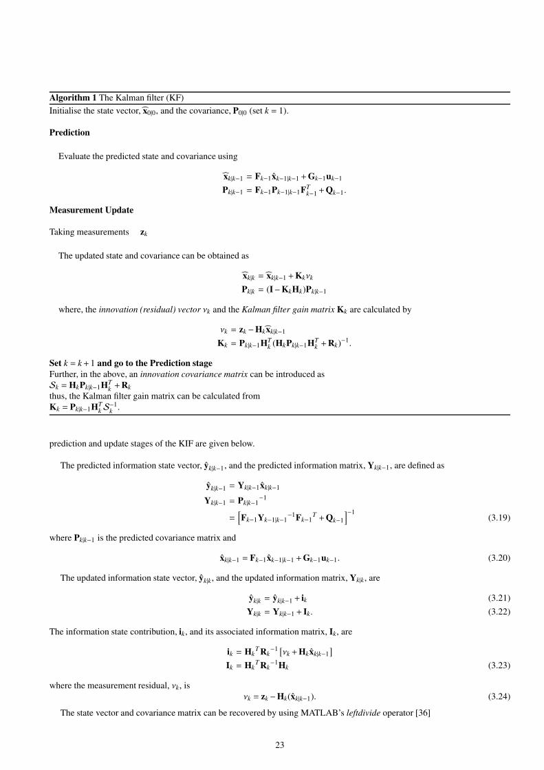
Algorithm 1 The Kalman filter (KF)
Initialise the state vector, x0|0, and the covariance, P0|0 (set k = 1).
Prediction
Evaluate the predicted state and covariance using
xk|k−1 = Fk−1xk−1|k−1 +Gk−1uk−1
Pk|k−1 = Fk−1Pk−1|k−1FTk−1+Qk−1.
Measurement Update
Taking measurements zk
The updated state and covariance can be obtained as
xk|k = xk|k−1 +Kkνk
Pk|k = (I−KkHk)Pk|k−1
where, the innovation (residual) vector νk and the Kalman filter gain matrix Kk are calculated by
νk = zk −Hkxk|k−1
Kk = Pk|k−1HTk (HkPk|k−1HT
k +Rk)−1.
Set k = k+1 and go to the Prediction stage
Further, in the above, an innovation covariance matrix can be introduced as
Sk =HkPk|k−1HTk+Rk
thus, the Kalman filter gain matrix can be calculated from
Kk = Pk|k−1HTkS−1
k.
prediction and update stages of the KIF are given below.
The predicted information state vector, yk|k−1, and the predicted information matrix, Yk|k−1, are defined as
yk|k−1 = Yk|k−1xk|k−1
Yk|k−1 = Pk|k−1−1
=[Fk−1Yk−1|k−1
−1Fk−1T +Qk−1
]−1(3.19)
where Pk|k−1 is the predicted covariance matrix and
xk|k−1 = Fk−1xk−1|k−1 +Gk−1uk−1. (3.20)
The updated information state vector, yk|k, and the updated information matrix, Yk|k, are
yk|k = yk|k−1 + ik (3.21)
Yk|k = Yk|k−1 + Ik. (3.22)
The information state contribution, ik, and its associated information matrix, Ik, are
ik = HkT Rk
−1 [νk +Hkxk|k−1
]
Ik = HkT Rk
−1Hk (3.23)
where the measurement residual, νk, is
νk = zk −Hk(xk|k−1). (3.24)
The state vector and covariance matrix can be recovered by using MATLAB’s leftdivide operator [36]
23

xk|k = Yk|k\yk|k (3.25)
Pk|k = Yk|k\In (3.26)
where In is the state vector sized identity matrix.
Initialisation in the information filter is easier than in the Kalman filter and the update stage of information filter is compu-
tationally simpler than the Kalman filter. KIF (and indeed the information filter forms of other filters) can be shown to be more
efficient than the Kalman filter in multiple sensor scenarios.
3.4 Discrete-timeH∞ filter
It is well understood that uncertainties are unavoidable in the operational environment of a real control system. The uncertainty
can be classified into two categories: unwanted yet unknown external signals and dynamic perturbations. The former includes
input and output disturbance (such as a gust on an aircraft), sensor noise and actuator noise, etc. The latter represents the
discrepancy between the mathematical model and the actual dynamics of the system in operation. A mathematical model
of any real system is always just an approximation of the true, physical reality of the system dynamics. Typical sources of the
discrepancy include unmodelled (usually of high-frequency nature) dynamics, neglected nonlinearities in the modelling process,
effects of deliberately reduced-order models, and system-parameter variations due to environmental changes and tear-and-wear
factors. These modelling errors may adversely affect the stability and performance level of a control system. The Kalman filter
discussed earlier assumes the process model has known dynamics and the noise sources have known statistics. However, due to
the very possible scenarios of uncertainties, these assumptions may limit the application of Kalman filters in real applications.
To overcome some of these limitations of Kalman filters, a few researchers have proposedH∞ filters [7, 12, 41, 84, 88, 98, 122].
This section presents a brief introduction to anH∞4 filter which minimises the worst-case estimation error. This is in contrast
to the Kalman filter which minimises the expected value of the variance of the estimation error. Furthermore, H∞ filtering
approach does not set any assumptions about the statistics of the process and measurement noises. For a detailed formulation
and derivation please see for example [35, 98, 104] or [100].
The discrete-time process and observation models can be written as
xk = Fk−1xk−1 +Gk−1uk−1 +wk−1, (3.27)
zk = Hkxk +vk, (3.28)
where k is the time index, xk is the state vector, uk the control input, zk the measurement vector, and wk−1 and vk are the process
and measurement noises. These model equations are almost the same as that of the Kalman filter described in Section 3.2.1;
except the assumption on noises. The noise terms wk−1 and vk may be random with possibly unknown statistics, or even they
may be deterministic. They may have a non-zero mean.
In aH∞ filter, instead of directly estimating the state one may estimate a linear combination of the states
nk = Lkxk. (3.29)
Of course, by replacing L with the identity matrix, one can directly estimate the state vector.
In the game theory approach ofH∞ filtering, the performance measure is given by
J∞ =
∑Nk=1‖nk − nk‖2Mk
‖x0 − x0‖2P−1
0
+∑N
k=1(‖wk‖2
Q−1k
+ ‖vk‖2R−1
k
)(3.30)
where P0, Qk, Rk, and Mk are symmetric, positive definite weighting matrices chosen by the user based on the problem at hand.
The norm notation used in this section is ‖e‖2S k= eT S ke.
In this dynamic game theory framework, there are essentially two players: the designer and the Nature. The designer’s goal
is to find the estimates of the error nk − nk so that the cost J∞ is minimised, while the Nature’s goal is to maximise J∞. The
numerator of J∞ can be viewed as the energy of the estimation error and the denominator can be considered as the energy of
the unknown disturbances. The Nature can simply put large magnitudes of wk, vk, and x0 to achieve its ultimate goal, and this
makes the game unfair to the designer. Thus, the J∞ is defined with (x0 − x0),wk, and vk in the denominator. Then, the Nature
4 H∞ filters minimizes the worst case energy gain from the noise input to the estimation error, which is equivalent to minimising the corresponding
H∞ norm.
24

needs to cleverly choose those disturbances in order to maximise nk − nk; likewise the designer also should be smart to find an
estimation strategy to minimise nk − nk.
The task of theH∞ filter is to minimise the state estimation error so that J∞ is bounded by a prescribed threshold under the
worst case wk, vk, and x0
supJ∞ < γ2 (3.31)
where “sup” stands for supremum, γ > 0 is the error attenuation parameter.
Based on Equation(3.31), the designer should find xk so that J∞ < γ2 holds for any disturbances in wk, vk, and x0. The best
the designer can do is to minimise J∞ under worst case disturbances, then the H∞ filter can be interpreted as the following
‘minmax’ problem
min max J∞xk wk ,vk ,x0
(3.32)
For detailed analysis and solution procedure of theH∞ filtering approach, please see [100] and [104]. In this section, we use
theH∞ filter algorithm given in [123], as the relevant equations in this reference are closely related to that of the Kalman filter.
The predicted state vector and auxiliary matrix ofH∞ filter are
xk|k−1 = Fk−1xk−1|k−1 +Gk−1uk−1
Pk|k−1 = Fk−1Pk−1|k−1FTk−1 +Qk−1
and the updated state and inverse of the updated auxiliary matrix can be obtained as
xk|k = xk|k−1 +K∞[zk −Hkxk|k−1] (3.33)
P−1k|k = P−1
k|k−1 +HTk R−1
k Hk −γ−2In (3.34)
where
K∞ = Pk|k−1HTk [HkPk|k−1HT
k +Rk]−1 (3.35)
and In denotes the identity matrix of dimension n×n.
AnH∞ filter can be summarised in Algorithm 2, that has a structure similar to that of the Kalman filter.
Algorithm 2H∞ Filter
Initialise the state vector, x0|0, and the auxiliary matrix, P0|0 (set k = 1).
Prediction
1: Evaluate the predicted state and auxiliary matrix using
xk|k−1 = Fk−1xk−1|k−1 +Gk−1uk−1
Pk|k−1 = Fk−1Pk−1|k−1FTk−1+Qk−1.
Measurement Update
1: The updated state and the inverse of auxiliary matrix can be obtained as
xk|k = xk|k−1 +K∞νk
P−1k|k = P−1
k|k−1 +HTk R−1
k Hk −γ−2In
where,
νk = zk −Hkxk|k−1
K∞ = Pk|k−1HTk (HkPk|k−1HT
k +Rk)−1
It is interesting to note that, for very high values of γ, the updated auxiliary matrix of theH∞ filter in Equation(3.34) and the
covariance matrix of the Kalman filter in Equation(3.18) are equivalent. Hence, the H∞ filter’s performance can be matched
with that of the Kalman filter, but the reverse is not true.
25

3.5 State estimation and control of a quadruple-tank system
In the previous sections, the Kalman and H∞ filters were discussed, along with the information filter. This section deals with
the combined state estimation and control problem for a quadruple-tank system using a Kalman filter, an information filter
and an H∞ filter. The controller design is based on the sliding mode control (SMC), which involves a stable sliding surface
design followed by a control law design to ensure the system states onto the chosen surface [8]. Combined SMC and state
estimators for the quadruple-tank are then to be presented. Such approaches can be explored for many other practical systems.
The basic structure of the approach is shown in Figure 3.1. In this section, firstly, a brief literature survey on quadruple-tank
system is given. The mathematical model of the quadruple-tank system is then presented, which is followed by SMC design
and combined SMC-state estimators, and ended by the closed-loop simulations. Figures will be included to show the simulation
results by using the Kalman filter and theH∞ filter.
Fig. 3.1: A combined SMC-H∞ filter approach.
3.5.1 Quadruple-tank system
The quadruple-tank considered here is an interesting multivariable plant consisting of four interconnected tanks and two pumps
[51] that some researchers have used it to explore different control and estimation methods. Decentralised proportional-integral
(PI) control, internal model control (IMC) andH∞ controllers have all been designed for the quadruple-tank system [112]. And,
it has been reported that the IMC and H∞ controllers provided better performance than the PI controller. Different nonlinear
model predictive controllers were also proposed in [80] and [92]. Also, the interconnection and damping assignment passivity
based control scheme for the quadruple-tank system was given in [52]. Furthermore, a nonlinear sliding mode controller (SMC)
with feedback linearisation was proposed and implemented in [14].
It is a well known fact that all the states are required for a state feedback controller design. However, in most of real-world,
practical applications, the states are not always available for feedback. Similarly, in the quadruple-tank system, only the first
two states are assumed to be accessible for feedback and hence either one has to rely on output feedback control methods or the
remaining two states are to be estimated for a state feedback design. The usage of an extended Kalman filter and high gain ob-
servers for the state estimation of a quadruple-tank system was given in [95] and state estimation in non-Gaussian domain using
particle filter was described in [47]. A very few researchers have demonstrated using combined controller-observer scheme for
the quadruple-tank. Though in [86], Kalman filter was used for the estimation of unavailable states of a quadruple-tank system
and the controller was based on PID and IMC.
In this section, the discrete-time SMC using the Kalman andH∞ filters, respectively, is to be designed for the quadruple-tank.
Nonlinear sliding surface proposed in [8] and [9] is considered to achieve better performance. The SMC for a quadruple-tank
was also reported in [14]. But, our approach is different from [14] in two aspects. In [14], the objective was to control just two
states and linear sliding surfaces were constructed using only the first two states. However, in this section the main emphasis is
to control all the four states and the nonlinear sliding surfaces are designed using complete state information. Secondly, SMC
given in Theorem 1 of [14] requires the full state information. Whereas, we have assumed only two states are available from
sensors and the complete state vector is estimated using Kalman andH∞ filters, respectively.
The quadruple-tank system is shown in Figure 3.2, which consists of four interconnected tanks, two pumps and two level
sensors. For more details, see [51] for the continuous time plant model. The quadruple-tank is discretised using Euler’s method
with sampling time of ∆T = 0.1s. The discrete-time nonlinear quadruple-tank model is
26

Fig. 3.2: Quadruple-Tank System [51].
xk+1=
x1k +∆T (− a1
A1
√2gx1k +
a3
A1
√2gx3k +
γ1k1
A1u1)
x2k +∆T (− a2
A2
√2g2k +
a4
A2
√2gx4k +
γ2k2
A2u2)
x3k +∆T (− a3
A3
√2gx2k +
(1−γ2)k2
A3u2)
x4k +∆T (− a4
A4
√2gx4k +
(1−γ1)k1
A4u1)
where, the state vector x, consisting of water levels of all tanks, is x = [x1, x2, x3, x4]T . The inputs are the voltages to the two
pumps, [u1,u2]T and the outputs are the voltages from the level measurements of the first two tanks. Ai is the cross section
of Tank i and ai is the cross section of outlet hole. The first input u1 directly affects the first and fourth states, whereas the
second input u2 has direct influence on the second and third states. The outputs are the measured level signals, kcx1 and kcx2.
The additive process and sensor noises are added to the state and output vectors, respectively. The parameter values used for
simulation are given in Table 3.1.
Parameters Values
A1, A3 (cm2) 28
A2, A4 (cm2) 32
a1, a3 (cm2) 0.071
a2, a4 (cm2) 0.057
kc (V/cm) 0.5
g (cm/s2) 981
Table 3.1: Quadruple-tank parameters.
27
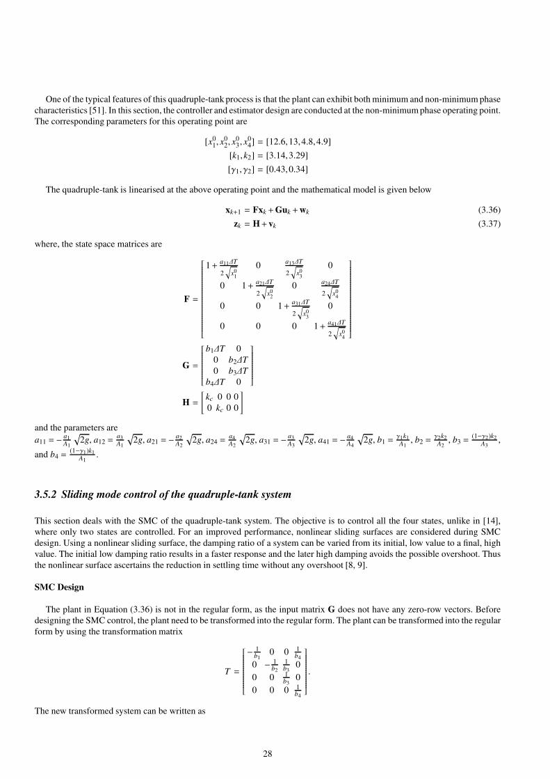
One of the typical features of this quadruple-tank process is that the plant can exhibit both minimum and non-minimum phase
characteristics [51]. In this section, the controller and estimator design are conducted at the non-minimum phase operating point.
The corresponding parameters for this operating point are
[x01, x
02, x
03, x
04] = [12.6,13,4.8,4.9]
[k1,k2] = [3.14,3.29]
[γ1,γ2] = [0.43,0.34]
The quadruple-tank is linearised at the above operating point and the mathematical model is given below
xk+1 = Fxk +Guk +wk (3.36)
zk = H+vk (3.37)
where, the state space matrices are
F =
1+a11∆T
2
√x0
1
0a13∆T
2
√x0
3
0
0 1+a21∆T
2
√x0
2
0a24∆T
2
√x0
4
0 0 1+a31∆T
2
√x0
3
0
0 0 0 1+a41∆T
2
√x0
4
G =
b1∆T 0
0 b2∆T
0 b3∆T
b4∆T 0
H =
[kc 0 0 0
0 kc 0 0
]
and the parameters are
a11 = − a1
A1
√2g, a12 =
a3
A1
√2g, a21 = − a2
A2
√2g, a24 =
a4
A2
√2g, a31 = − a3
A3
√2g, a41 = − a4
A4
√2g, b1 =
γ1k1
A1, b2 =
γ2k2
A2, b3 =
(1−γ2)k2
A3,
and b4 =(1−γ1)k1
A1.
3.5.2 Sliding mode control of the quadruple-tank system
This section deals with the SMC of the quadruple-tank system. The objective is to control all the four states, unlike in [14],
where only two states are controlled. For an improved performance, nonlinear sliding surfaces are considered during SMC
design. Using a nonlinear sliding surface, the damping ratio of a system can be varied from its initial, low value to a final, high
value. The initial low damping ratio results in a faster response and the later high damping avoids the possible overshoot. Thus
the nonlinear surface ascertains the reduction in settling time without any overshoot [8, 9].
SMC Design
The plant in Equation (3.36) is not in the regular form, as the input matrix G does not have any zero-row vectors. Before
designing the SMC control, the plant need to be transformed into the regular form. The plant can be transformed into the regular
form by using the transformation matrix
T =
− 1b1
0 0 1b4
0 − 1b2
1b3
0
0 0 1b3
0
0 0 0 1b4
.
The new transformed system can be written as
28
yk+1 = (TFT−1)yk +TGuk +TGwk (3.38)
where yk = Txk and the system can be further expressed as
yk+1 =
[yu,k+1
yl,k+1
]=
[y11 y12
y21 y22
][yu,k
yl,k
]+
[0
Gl
]uk +
[0
Gl
]wk (3.39)
where
y11 =
1+a11∆T
2
√x0
1
0
0 1+a21∆T
2
√x0
2
y12 =
a13b3∆T
2b1
√x0
3
∆T2
(a41√
x04
− a11√x0
1
)
∆T2
(a31√
x03
− a21√x0
2
)a24b4∆T
2b2
√x0
4
y21 =
[0 0
0 0
]
y22 =
1+a31∆T
2
√x0
3
0
0 1+a41∆T
2
√x0
4
Gl =
[0 ∆T
∆T 0
].
Nonlinear sliding surface design
The performance of the SMC-based, closed-loop system can be enhanced by using the nonlinear surfaces [8, 9] and hence
in the present book a nonlinear sliding surface is to be adopted.
Let the nonlinear sliding surface [8] be
sk = cTk yk (3.40)
where
cTk = [K−ψ(zk)yT
12P(y11−y12K) I2] (3.41)
and I2 is the second order identity matrix.
The gain matrix,
K =
[−0.66651 −0.2026
0.06417 −0.6641
](3.42)
is obtained by solving the linear quadratic regulator (LQR) problem for y11 and y12, such that (y11 −y12K) have stable eigen-
values (i.e. in the open, left-half complex plane). The weighting matrices considered for the LQR design are chosen as
Qlqr =
[10 0
0 10
]and Rlqr =
[10 0
0 10
].
The matrix P, required for Equation (3.41) is obtained by solving the following Lyapunov equation
P = (y11−y12K)T P(y11−y12K)+W. (3.43)
By selecting W as I2, the corresponding P matrix is
[1223.39 −32.47
−32.57 162.17
].
The nonlinear function, ψ(zk), can be chosen as [8]
29

ψ(zk) =
−β1e
−m1 |x01,k−1
|0
0 −β2e−m2 |x0
2,k−1|
(3.44)
where β1, β2, m1 and m2 are the tuning parameters. These parameters are selected as unity and ψ(zk) is chosen such that it
satisfies the below condition [9, 24]
2ψ(zk)+ψ(zk)yT12Py12ψ(zk) ≤ 0. (3.45)
Control law
Now the control law will be derived. From Equation (3.40), sk+1 can be written as
sk+1 = cTk+1yk+1
sk+1 = cTk+1Txk+1. (3.46)
By using Equation (3.36) and Equation (3.46), sk+1 can be written as
sk+1 = cTk+1TFxk + cT
k+1TGuk + cTk+1TGwk. (3.47)
In the discrete-time sliding mode control, one of the objectives is to achieve the sliding surfaces, sk = 0 in a finite time [8].
This can be achieved by an equivalent control law [111] by setting
sk+1 = 0. (3.48)
By using Equation (3.47) and Equation (3.48), the control law can be derived as
cTk+1TFxk + cT
k+1TGuk + cTk+1TGwk = 0 (3.49)
and
uk = −(cTk+1TG)−1(cT
k+1TFxk + cTk+1TGwk). (3.50)
The aforementioned control law contains uncertain terms or process noises. In general these uncertain terms are unknown.
They can however be replaced by the average of known bounds of these terms [9]. The modified control law can be written as
uk = −(cTk+1TG)−1(cT
k+1TFxk +dm). (3.51)
where dm is the average of the lower and upper bounds of cTk+1
TGwk.
From Equation (3.51), it can be seen that the control law at the kth time instant requires the information at k+1th time instant,
and in general this is not feasible. However, from Equation (3.41) and Equation (3.44), only the output information at kth instant
(x1,k and x2,k) is required to find ck+1 and hence the control input, uk, can be evaluated using just the output information at kth
instant.
Stability of the nonlinear sliding surface
From Equation (3.39),
yu,k+1 = y11yu,k +y12yl,k (3.52)
During the sliding phase, sk = 0, and hence Equation (3.40) can be written as
cTk yk = 0 (3.53)
⇒[K−ψ(zk)yT
12Pyeq I2
] [yu,k ylk
]T= 0 (3.54)
⇒ yl,k = −[K−ψ(zk)yT12Pyeq]yu,k (3.55)
where yeq = y11 −y12K.
From Equation (3.52) and Equation (3.55),
30

yu,k+1 = y11yu,k +y12(−[K−ψ(zk)yT12Pyeq])yu,k (3.56)
= (y11−y12K)yu,k +y12ψ(zk)yT12Pyeqyu,k (3.57)
= (y12ψ(zk)yT12P+ I)yeqyu,k. (3.58)
The stability of the nonlinear sliding surface can be proved by using the Lyapunov theory. It is assumed that the Lyapunov
function for the system defined in Equation (3.58) is
Vk = yTu,kPyu,k. (3.59)
The increment of Vk is
Vk = Vk+1−Vk (3.60)
= yTu,k+1Pyu,k+1 −yT
u,kPyu,k
= (yTu,kyT
eq+yTu,kyT
eqPy12ψ(zk)yT12)P(yeqyu,k +y12ψ(zk)yT
12Pyeqyu,k)−yTu,kPyu,k
= yTu,kyT
eqPyeqyu,k +yTu,kyT
eqPy12ψ(zk)yT12Pyeqyu,k +yT
u,kyTeqPy12ψ(zk)yT
12Pyeqyu,k +
yTu,kyT
eqPy12ψ(zk)yT12Py12ψ(zk)yT
12Pyeqyu,k −yTu,kPyu,k
= −yTu,k(P−yT
eqPyeq)yu,k +yTu,kyT
eqPy12[2ψ(zk)+ψ(zk)yT12Py12ψ(zk)]yT
12Pyeqyu,k
= −yTu,kWyu,k +MT [2ψ(zk)+ψ(zk)yT
12Py12ψ(zk)]M (3.61)
where M = yTu,k
yTeqPy12.
From Equation (3.45) and Equation (3.61), one can write
∇V ≤ −yTu,kWyu,k. (3.62)
Since the increment of the Lyapunov function is of negative definite, the equilibrium point for Equation (3.58) is stable, and
hence the designed nonlinear sliding surface is stable. In a similar way by constructing the Lyapunov function of the sliding
surface, sk+1, the increment of the Lyapunov function can be easily shown to be negative definite which in turn proves the
existence of the sliding mode [9].
3.5.3 Combined schemes: Simulations and results
By using the filter algorithms described in Section 3.2 and Section 3.4, all the four states of the quadruple-tank can be estimated
by using x1 and x2 . One may note that, the control input u required for the quadruple-tank is obtained from SMC controller
given in Section 3.5.2. This proposed scheme for the quadruple-tank system is shown in Figure 3.3. The process noise is added
to all the four states, whereas the measurement noise is added to the last two states only; the quadruple-tank block in Figure 3.3
assumed to have additive noises and hence separate noises are not added in the block diagram. The usage of theH∞ filter in this
work is required for two purposes; it is used to estimate the two unavailable states, and to inherently filter out the process and
sensor noises. One may note that in this work although the first two states of the quadruple-tank are available from the sensors,
we are still using the full order state estimation rather than a reduced order state estimation. The first two estimated states are
less noisy than actual measured states and are beneficial for the state feedback SMC control design.
This section describes the various simulations done for closed loop quadruple-tank system. Although, the controller and
estimator designs are conducted for the linearised model, the simulations in this section are performed on the full nonlinear
model. The SMC given in Section 3.5.2 and the estimator in Sections 3.2 and 3.4 are considered in the simulations. The first
two sensed states from quadruple-tank are given to the filters, which then estimates all the four states. These estimated states
from estimators are used by the SMC, which then provides the input to the quadruple-tank system. The initial values of the
plant are perturbed by +15% of their nominal values, and the objective is to bring back the perturbed states to the actual initial
conditions. The chosen initial covariance matrix, P0|0, is
31
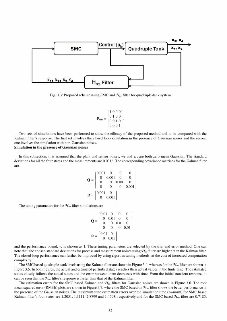
Fig. 3.3: Proposed scheme using SMC andH∞ filter for quadruple-tank system
P0|0 =
1 0 0 0
0 1 0 0
0 0 1 0
0 0 0 1
.
Two sets of simulations have been performed to show the efficacy of the proposed method and to be compared with the
Kalman filter’s response. The first set involves the closed loop simulation in the presence of Gaussian noises and the second
one involves the simulation with non-Gaussian noises.
Simulation in the presence of Gaussian noises
In this subsection, it is assumed that the plant and sensor noises, wk and vk, are both zero-mean Gaussian. The standard
deviations for all the four states and the measurements are 0.0316. The corresponding covariance matrices for the Kalman filter
are
Q =
0.001 0 0 0
0 0.001 0 0
0 0 0.001 0
0 0 0 0.001
R =
[0.001 0
0 0.001
].
The tuning parameters for theH∞ filter simulations are
Q =
0.01 0 0 0
0 0.01 0 0
0 0 0.01 0
0 0 0 0.01
R =
[0.01 0
0 0.01
].
and the performance bound, γ, is chosen as 1. These tuning parameters are selected by the trial and error method. One can
note that, the chosen standard deviations for process and measurement noises usingH∞ filter are higher than the Kalman filter.
The closed-loop performance can further be improved by using rigorous tuning methods; at the cost of increased computation
complexity.
The SMC based quadruple-tank levels using the Kalman filter are shown in Figure 3.4, whereas for theH∞ filter are shown in
Figure 3.5. In both figures, the actual and estimated perturbed states reaches their actual values in the finite time. The estimated
states closely follows the actual states and the error between them decreases with time. From the initial transient response, it
can be seen that theH∞ filter’s response is faster than that of the Kalman filter.
The estimation errors for the SMC based Kalman and H∞ filters for Gaussian noises are shown in Figure 3.6. The root
mean squared error (RMSE) plots are shown in Figure 3.7, where the SMC based onH∞ filter shows the better performance in
the presence of the Gaussian noises. The maximum state estimation errors over the simulation time (∞-norm) for SMC based
Kalman filter’s four states are 1.2051, 1.3111, 2.8799 and 1.4693, respectively and for the SMC based H∞ filter are 0.7185,
32

0 50 100 150 20010
12
14
16
Time (s)
h1(c
m)
0 50 100 150 20012
13
14
15
Time (s)
h2(c
m)
0 50 100 150 200−5
0
5
10
Time (s)
h3(c
m)
0 50 100 150 2000
2
4
6
Time (s)
h4(c
m)
Actual SMC−KF
Fig. 3.4: Actual and estimated states of the quadruple-tank using the Kalman filter in the presence of Gaussian noises.
33
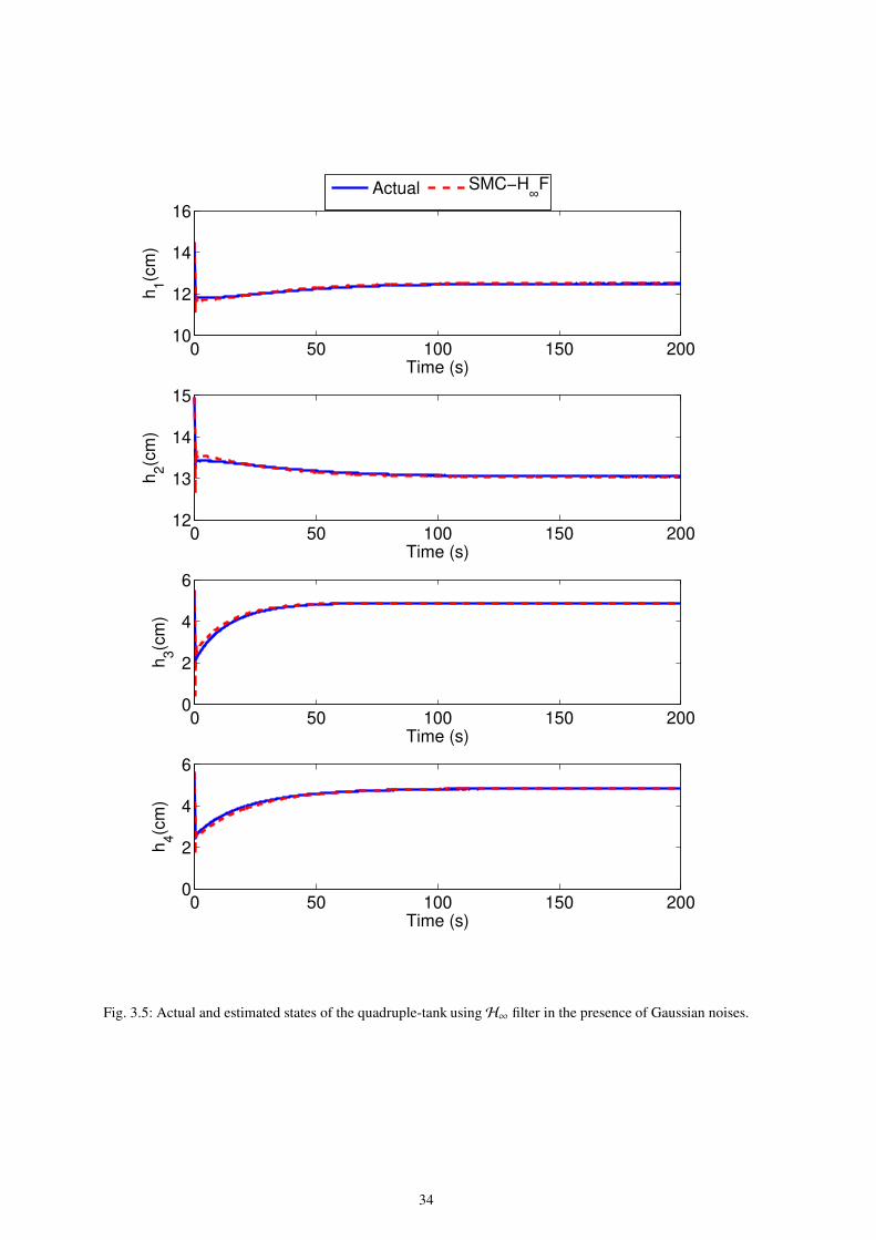
0 50 100 150 20010
12
14
16
Time (s)
h1(c
m)
0 50 100 150 20012
13
14
15
Time (s)
h2(c
m)
0 50 100 150 2000
2
4
6
Time (s)
h3(c
m)
0 50 100 150 2000
2
4
6
Time (s)
h4(c
m)
Actual SMC−H∞F
Fig. 3.5: Actual and estimated states of the quadruple-tank usingH∞ filter in the presence of Gaussian noises.
34

0 50 100 150 200−2
0
2
Time (s)
h1(c
m)
0 50 100 150 200−2
0
2
Time (s)
h2(c
m)
0 50 100 150 200−5
0
5
Time (s)
h3(c
m)
0 50 100 150 200−2
0
2
Time (s)
h4(c
m)
SMC−KF estimation error SMC−H∞F estimation error
Fig. 3.6: Estimation errors for the quadruple-tank using Kalman andH∞ filters in the presence of Gaussian noises.
0.7254, 1.6648 and 0.8921, respectively. In the simulations, the quadruple-tank is excited by Gaussian noises for both the
Kalman andH∞ filters. In the Kalman filter, if the standard deviation of noises once fixed then the corresponding covariances
are the square of the standard deviations. However, in theH∞ filter, there is a freedom to select tuning parameters irrespective
of the noises. Both Kalman and H∞ filters’ performances can further improved by tuning Q and R. The results in this section
are shown for the full nonlinear model. When the same simulations are repeated with linear open-loop plant model, the Kalman
filter’s response is better than theH∞ filter’s response, as the Kalman filter is the optimal estimator for linear-Gaussian systems.
Simulation in the presence of non-Gaussian noises
In most of real-life applications, the assumption of zero-mean and Gaussian noises may not be valid. To validate the proposed
approach, non-zero mean and non-Gaussian noises are considered for the simulations. The process and measurement noises are
wk =
0.01+0.01× sin(0.1k)
0.01+0.01× sin(0.1k)
0.01+0.01× sin(0.1k)
0.01+0.01× sin(0.1k)
vk =
[0.01+0.01× sin(0.1k)
0.01+0.01× sin(0.1k)
].
35
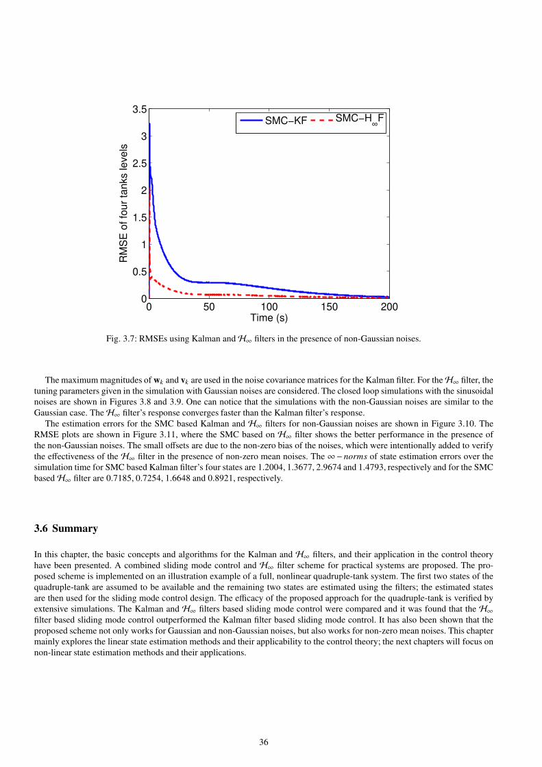
0 50 100 150 2000
0.5
1
1.5
2
2.5
3
3.5
Time (s)
RM
SE
of
fou
r ta
nks le
ve
ls
SMC−KF SMC−H∞F
Fig. 3.7: RMSEs using Kalman andH∞ filters in the presence of non-Gaussian noises.
The maximum magnitudes of wk and vk are used in the noise covariance matrices for the Kalman filter. For theH∞ filter, the
tuning parameters given in the simulation with Gaussian noises are considered. The closed loop simulations with the sinusoidal
noises are shown in Figures 3.8 and 3.9. One can notice that the simulations with the non-Gaussian noises are similar to the
Gaussian case. TheH∞ filter’s response converges faster than the Kalman filter’s response.
The estimation errors for the SMC based Kalman and H∞ filters for non-Gaussian noises are shown in Figure 3.10. The
RMSE plots are shown in Figure 3.11, where the SMC based on H∞ filter shows the better performance in the presence of
the non-Gaussian noises. The small offsets are due to the non-zero bias of the noises, which were intentionally added to verify
the effectiveness of the H∞ filter in the presence of non-zero mean noises. The ∞− norms of state estimation errors over the
simulation time for SMC based Kalman filter’s four states are 1.2004, 1.3677, 2.9674 and 1.4793, respectively and for the SMC
basedH∞ filter are 0.7185, 0.7254, 1.6648 and 0.8921, respectively.
3.6 Summary
In this chapter, the basic concepts and algorithms for the Kalman and H∞ filters, and their application in the control theory
have been presented. A combined sliding mode control and H∞ filter scheme for practical systems are proposed. The pro-
posed scheme is implemented on an illustration example of a full, nonlinear quadruple-tank system. The first two states of the
quadruple-tank are assumed to be available and the remaining two states are estimated using the filters; the estimated states
are then used for the sliding mode control design. The efficacy of the proposed approach for the quadruple-tank is verified by
extensive simulations. The Kalman and H∞ filters based sliding mode control were compared and it was found that the H∞filter based sliding mode control outperformed the Kalman filter based sliding mode control. It has also been shown that the
proposed scheme not only works for Gaussian and non-Gaussian noises, but also works for non-zero mean noises. This chapter
mainly explores the linear state estimation methods and their applicability to the control theory; the next chapters will focus on
non-linear state estimation methods and their applications.
36

0 50 100 150 20010
12
14
16
Time (s)
h1(c
m)
0 50 100 150 20012
13
14
15
Time (s)
h2(c
m)
0 50 100 150 200−5
0
5
10
Time (s)
h3(c
m)
0 50 100 150 2000
2
4
6
Time (s)
h4(c
m)
Actual SMC−KF
Fig. 3.8: Actual and estimated states of the quadruple-tank using the Kalman filter in the presence of non-Gaussian noises.
37

0 50 100 150 20010
12
14
16
Time (s)
h1(c
m)
0 50 100 150 20012
13
14
15
Time (s)
h2(c
m)
0 50 100 150 2000
2
4
6
Time (s)
h3(c
m)
0 50 100 150 2000
2
4
6
Time (s)
h4(c
m)
Actual SMC−H∞F
Fig. 3.9: Actual and estimated states of the quadruple-tank usingH∞ filter in the presence of non-Gaussian noises.
38

0 50 100 150 200−2
0
2
Time (s)
h1(c
m)
0 50 100 150 200−2
0
2
Time (s)
h2(c
m)
0 50 100 150 200−5
0
5
Time (s)
h3(c
m)
0 50 100 150 200−2
0
2
Time (s)
h4(c
m)
SMC−KF estimation error SMC−H∞F estimation error
Fig. 3.10: Estimation errors for the quadruple-tank using Kalman andH∞ filters in the presence of non-Gaussian noises.
39

0 50 100 150 2000
0.5
1
1.5
2
2.5
3
3.5
Time (s)
RM
SE
of fo
ur
tanks levels
SMC−KF SMC−H∞F
Fig. 3.11: RMSEs using Kalman andH∞ filters in the presence of non-Gaussian noises.
40

Chapter 4
Jacobian-based Nonlinear State Estimation
4.1 Introductory remarks
Nonlinearity is one of the most challenging issues in controllers and observers design. Most of the practical systems are inher-
ently nonlinear [106], [61]. On the other hand, most control schemes and observer/estimater design methods used widely are for
linear systems and are therefore not applicable in practice because of the existence of nonlinearities. This chapter deals with the
state estimation methods for nonlinear systems stemmed from, however, linear estimator design ideas. Namely, the extensions
of Kalman filter, information filter and anH∞ filter to nonlinear systems will be discussed in this chapter. These extensions are
based on the first order Taylor’s series expansion of the nonlinear process and/or measurement dynamics. The idea is, in some
key steps of estimation, to replace the nonlinear process and/or measurement models with their corresponding Jacobians. The
three filters to be discussed in this chapter are therefore the extended Kalman filter (EKF), extended information filter (EIF) and
extendedH∞ filter (EH∞F).
4.2 Extended Kalman filter
Consider the following discrete, nonlinear process and measurement models
xk = f(xk−1,uk−1)+wk−1 (4.1)
zk = h(xk,uk)+vk (4.2)
where k is the time index, xk ∈ Rn is the state vector, uk the input variable, zk the measurement (measurable output), wk−1
the process noise and vk the measurement noise. The noises wk−1 and vk are assumed to be zero mean, Gaussian-distributed,
random variables with covariances of Qk−1 and Rk, respectively.
Similar to the Kalman filter, the extended Kalman filter (EKF) is also a recursive process consisting of prediction and
measurement update but it requires Jacobians of the process and measurement dynamics.
To deal with nonlinear functions (or so-called nonlinear mappings), a natural and logical idea is to linearise the nonlinear
functions and then to consider the “approximated” versions, i.e. the linearised ones, of the nonlinear functions instead. In doing
so, the approximation should be kept as close as possible to the original function, for obvious reasons. In the estimation of
nonlinear systems states, therefore, it is not directly to linearise the functions f(·, ·) and h(·, ·) in (4.1) and (4.2), respectively, at
chosen equilibrium points and then to apply linear state estimation algorithms. Instead, to employ the nonlinear functions as
longer as possible in the estimation and only to use the approximations of nonlinear functions when absolutely necessary.
In EKF, prediction of the state vector and covariance matrix can be calculated from
xk|k−1 = f(xk−1|k−1,uk−1) (4.3)
Pk|k−1 = ∇fxPk−1|k−1∇fTx +Qk−1 (4.4)
where, ∇fx is the Jacobian of function f with respect to the state variable x, obtained from the Taylor expansion series of f.
The updated state and covariance can therefore be obtained as
xk|k = xk|k−1 +Kk[zk −h(xk|k−1,uk)] (4.5)
Pk|k = (In−Kk∇hx)Pk|k−1 (4.6)
41
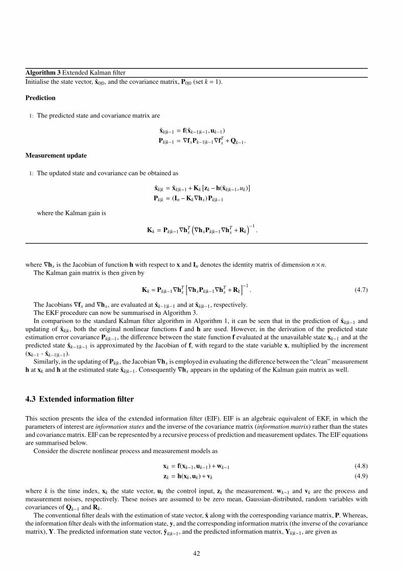
Algorithm 3 Extended Kalman filter
Initialise the state vector, x0|0, and the covariance matrix, P0|0 (set k = 1).
Prediction
1: The predicted state and covariance matrix are
xk|k−1 = f(xk−1|k−1,uk−1)
Pk|k−1 = ∇fxPk−1|k−1∇fTx +Qk−1.
Measurement update
1: The updated state and covariance can be obtained as
xk|k = xk|k−1 +Kk
[zk −h(xk|k−1,uk)
]
Pk|k = (In−Kk∇hx)Pk|k−1
where the Kalman gain is
Kk = Pk|k−1∇hTx
(∇hxPk|k−1∇hT
x +Rk
)−1.
where ∇hx is the Jacobian of function h with respect to x and In denotes the identity matrix of dimension n×n.
The Kalman gain matrix is then given by
Kk = Pk|k−1∇hTx
[∇hxPk|k−1∇hT
x +Rk
]−1. (4.7)
The Jacobians ∇fx and ∇hx, are evaluated at xk−1|k−1 and at xk|k−1, respectively.
The EKF procedure can now be summarised in Algorithm 3.
In comparison to the standard Kalman filter algorithm in Algorithm 1, it can be seen that in the prediction of xk|k−1 and
updating of xk|k, both the original nonlinear functions f and h are used. However, in the derivation of the predicted state
estimation error covariance Pk|k−1, the difference between the state function f evaluated at the unavailable state xk−1 and at the
predicted state xk−1|k−1 is approximated by the Jacobian of f, with regard to the state variable x, multiplied by the increment
(xk−1 - xk−1|k−1).
Similarly, in the updating of Pk|k, the Jacobian∇hx is employed in evaluating the difference between the “clean” measurement
h at xk and h at the estimated state xk|k−1. Consequently ∇hx appears in the updating of the Kalman gain matrix as well.
4.3 Extended information filter
This section presents the idea of the extended information filter (EIF). EIF is an algebraic equivalent of EKF, in which the
parameters of interest are information states and the inverse of the covariance matrix (information matrix) rather than the states
and covariance matrix. EIF can be represented by a recursive process of prediction and measurement updates. The EIF equations
are summarised below.
Consider the discrete nonlinear process and measurement models as
xk = f(xk−1,uk−1)+wk−1 (4.8)
zk = h(xk,uk)+vk (4.9)
where k is the time index, xk the state vector, uk the control input, zk the measurement. wk−1 and vk are the process and
measurement noises, respectively. These noises are assumed to be zero mean, Gaussian-distributed, random variables with
covariances of Qk−1 and Rk.
The conventional filter deals with the estimation of state vector, x along with the corresponding variance matrix, P. Whereas,
the information filter deals with the information state, y, and the corresponding information matrix (the inverse of the covariance
matrix), Y. The predicted information state vector, yk|k−1, and the predicted information matrix, Yk|k−1, are given as
42

yk|k−1 = Yk|k−1xk|k−1 (4.10)
Yk|k−1 = P−1k|k−1
=[∇fxY−1
k−1|k−1∇fTx +Qk−1
]−1(4.11)
where Pk|k−1 is the predicted covariance matrix and
xk|k−1 = f(xk−1|k−1,uk−1). (4.12)
The updated information state vector, yk|k, and the updated information matrix, Yk|k, are
yk|k = yk|k−1 + ik (4.13)
Yk|k = Yk|k−1 + Ik. (4.14)
The information state contribution, ik, and its associated information matrix, Ik, are
ik = ∇hTx R−1
k
[νk +∇hxxk|k−1
](4.15)
Ik = ∇hTx R−1
k ∇hx (4.16)
where the measurement residual, νk, is
νk = zk −h(xk|k−1,uk) (4.17)
and ∇fx, and ∇hx are the Jacobians of f and h evaluated at the latest available state (Jacobians for prediction and update
equations are evaluated at xk−1|k−1 and xk|k−1, respectively).
One of the key advantages of the information filter over the Kalman filter is during the update stage, where the updated
information state and information matrix can be obtained by simply adding the associated information contributions to the
predicted information state and information matrix. Detailed derivation can be found in [83].
For the extended information filter, recovery of state and covariance matrices are required at different stages and is still an
active research area [55], [119], [36], [46]. The state vector and covariance matrix can be recovered by using left division 1 [36]
xk|k = Yk|k\yk|k (4.18)
Pk|k = Yk|k\In (4.19)
where In is the state vector sized identity matrix.
Initialisation in the information filter is easier than that in the Kalman filter and the update stage of information filter is
computationally simpler than that of the Kalman filter. EIF can be shown to be more efficient than the EKF. But some of the
drawbacks inherent in the EKF still affect the EIF. These include the nontrivial nature of the derivations of the Jacobian matrices
(and computation) and linearisation instability [83].
Since the EIF is an alternate form of EKF, the simulation results for the EIF is not too different to the one given in Figs. 4.1
and 4.2. However, the key advantage of the EIF is its usage in multi-sensor estimation; that will be further demonstrated in later
chapters.
4.4 Extended H∞ filter
This section presents the extendedH∞ filter (EH∞F). As discussed previously about the linear systems, the stochastic properties
of the noises affecting the model and output dynamics may not be exactly known. Hence, the Kalman filters, either the standard
or extended versions, will not be applicable in such cases. Therefore, H∞ filters could be a tool worth trying. The H∞ filters
do not need to assume that the process and measurement noises be Gaussian. Furthermore, the H∞ filters could tolerate a
certain degree of dynamic uncertainties in the process and measurement models. Similar to the linear case, the extended H∞filter (EH∞F) minimises the expected value of the variance of the estimation error and uses the Jacobian to approximate the
differences of the process (measurement) function evaluated at the unavailable state variable xk−1 (xk) and at the predicted state
xk−1|k−1 (xk|k−1).
Consider the discrete-time process and observation models written as
1 x = A\B solves the least square solution for Ax = B such that ‖Ax−b‖ is minimal.
43
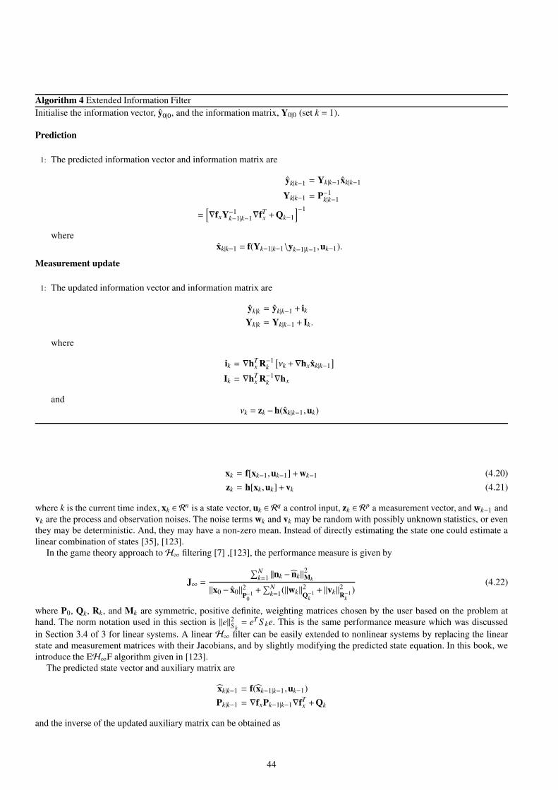
Algorithm 4 Extended Information Filter
Initialise the information vector, y0|0, and the information matrix, Y0|0 (set k = 1).
Prediction
1: The predicted information vector and information matrix are
yk|k−1 = Yk|k−1xk|k−1
Yk|k−1 = P−1k|k−1
=[∇fxY−1
k−1|k−1∇fTx +Qk−1
]−1
where
xk|k−1 = f(Yk−1|k−1\yk−1|k−1,uk−1).
Measurement update
1: The updated information vector and information matrix are
yk|k = yk|k−1 + ik
Yk|k = Yk|k−1 + Ik.
where
ik = ∇hTx R−1
k
[νk +∇hxxk|k−1
]
Ik = ∇hTx R−1
k ∇hx
and
νk = zk −h(xk|k−1,uk)
xk = f[xk−1,uk−1]+wk−1 (4.20)
zk = h[xk,uk]+vk (4.21)
where k is the current time index, xk ∈ Rn is a state vector, uk ∈ Rq a control input, zk ∈ Rp a measurement vector, and wk−1 and
vk are the process and observation noises. The noise terms wk and vk may be random with possibly unknown statistics, or even
they may be deterministic. And, they may have a non-zero mean. Instead of directly estimating the state one could estimate a
linear combination of states [35], [123].
In the game theory approach toH∞ filtering [7] ,[123], the performance measure is given by
J∞ =
∑Nk=1 ‖nk − nk‖2Mk
‖x0 − x0‖2P−1
0
+∑N
k=1(‖wk‖2
Q−1k
+ ‖vk‖2R−1
k
)(4.22)
where P0, Qk, Rk, and Mk are symmetric, positive definite, weighting matrices chosen by the user based on the problem at
hand. The norm notation used in this section is ‖e‖2S k= eT S ke. This is the same performance measure which was discussed
in Section 3.4 of 3 for linear systems. A linear H∞ filter can be easily extended to nonlinear systems by replacing the linear
state and measurement matrices with their Jacobians, and by slightly modifying the predicted state equation. In this book, we
introduce the EH∞F algorithm given in [123].
The predicted state vector and auxiliary matrix are
xk|k−1 = f(xk−1|k−1,uk−1)
Pk|k−1 = ∇fxPk−1|k−1∇fTx +Qk
and the inverse of the updated auxiliary matrix can be obtained as
44
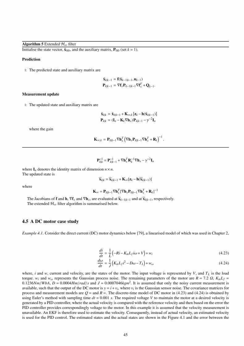
Algorithm 5 ExtendedH∞ filter
Initialise the state vector, x0|0, and the auxiliary matrix, P0|0 (set k = 1).
Prediction
1: The predicted state and auxiliary matrix are
xk|k−1 = f(xk−1|k−1,uk−1)
Pk|k−1 = ∇fxPk−1|k−1∇fTx +Qk−1.
Measurement update
1: The updated state and auxiliary matrix are
xk|k = xk|k−1 +K∞,k[zk −h(xk|k−1)
]
Pk|k = (In −Kk∇hx)Pk|k−1 −γ−2In
where the gain
K∞,k = Pk|k−1∇hTx
(∇hxPk|k−1∇hT
x +Rk
)−1.
P−1k|k = P−1
k|k−1 +∇hTx R−1
k ∇hx −γ−2In
where In denotes the identity matrix of dimension n×n.
The updated state is
xk|k = xk|k−1 +K∞[zk −h(xk|k−1)]
where
K∞ = Pk|k−1∇hTx [∇hxPk|k−1∇hT
x +Rk]−1
The Jacobians of f and h, ∇fx and ∇hx, are evaluated at xk−1|k−1 and at xk|k−1, respectively.
The extendedH∞ filter algorithm is summarised below.
4.5 A DC motor case study
Example 4.1. Consider the direct current (DC) motor dynamics below [79], a linearised model of which was used in Chapter 2,
di
dt=
1
L
(−Ri−KmL f iω+V
)+wi (4.23)
dω
dt=
1
J
(KmL f i2−Dω−TL
)+wω (4.24)
where, i and w, current and velocity, are the states of the motor. The input voltage is represented by V , and TL is the load
torque. wi and wω represents the Gaussian process noise. The remaining parameters of the motor are R = 7.2 Ω, KmL f =
0.1236Nm/WbA, D = 0.0004Hm/rad/s and J = 0.0007046kgm2. It is assumed that only the noisy current measurement is
available, such that the output of the DC motor is y = i+ vi, where vi is the Gaussian sensor noise. The covariance matrices for
process and measurement models are Q = and R =. The discrete-time model of DC motor in (4.23) and (4.24) is obtained by
using Euler’s method with sampling time dt = 0.001 s. The required voltage V to maintain the motor at a desired velocity is
generated by a PID controller, where the actual velocity is compared with the reference velocity and then based on the error the
PID controller provides correspondingly voltage to the motor. In this example it is assumed that the velocity measurement is
unavailable. An EKF is therefore used to estimate the velocity. Consequently, instead of actual velocity, an estimated velocity
is used for the PID control. The estimated states and the actual states are shown in the Figure 4.1 and the error between the
45
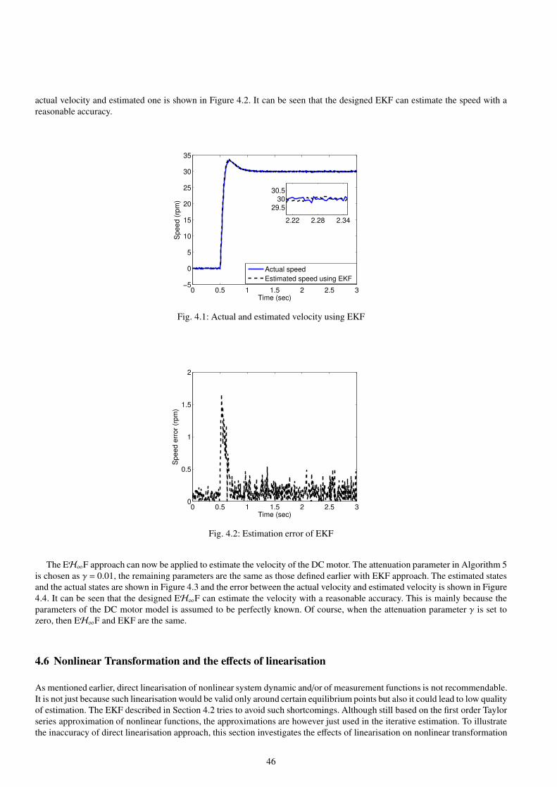
actual velocity and estimated one is shown in Figure 4.2. It can be seen that the designed EKF can estimate the speed with a
reasonable accuracy.
0 0.5 1 1.5 2 2.5 3−5
0
5
10
15
20
25
30
35
Time (sec)
Speed (
rpm
)
Actual speed
Estimated speed using EKF
2.22 2.28 2.34
29.5
30
30.5
Fig. 4.1: Actual and estimated velocity using EKF
0 0.5 1 1.5 2 2.5 30
0.5
1
1.5
2
Time (sec)
Speed e
rror
(rpm
)
Fig. 4.2: Estimation error of EKF
The EH∞F approach can now be applied to estimate the velocity of the DC motor. The attenuation parameter in Algorithm 5
is chosen as γ = 0.01, the remaining parameters are the same as those defined earlier with EKF approach. The estimated states
and the actual states are shown in Figure 4.3 and the error between the actual velocity and estimated velocity is shown in Figure
4.4. It can be seen that the designed EH∞F can estimate the velocity with a reasonable accuracy. This is mainly because the
parameters of the DC motor model is assumed to be perfectly known. Of course, when the attenuation parameter γ is set to
zero, then EH∞F and EKF are the same.
4.6 Nonlinear Transformation and the effects of linearisation
As mentioned earlier, direct linearisation of nonlinear system dynamic and/or of measurement functions is not recommendable.
It is not just because such linearisation would be valid only around certain equilibrium points but also it could lead to low quality
of estimation. The EKF described in Section 4.2 tries to avoid such shortcomings. Although still based on the first order Taylor
series approximation of nonlinear functions, the approximations are however just used in the iterative estimation. To illustrate
the inaccuracy of direct linearisation approach, this section investigates the effects of linearisation on nonlinear transformation
46

0 0.5 1 1.5 2 2.5 3−5
0
5
10
15
20
25
30
35
Time (sec)
Speed (
rpm
)
Actual speed
Estimated speed using EH∞F
Fig. 4.3: Actual and estimated velocity using EH∞F
0 0.5 1 1.5 2 2.5 30
0.5
1
1.5
2
Time (sec)
EH
∞F
speed e
rror
(rpm
)
Fig. 4.4: Estimation error using EH∞F
of polar to cartesian coordinates and analyses the corresponding estimation error. The similar discussion has been considered in
[53, 54, 104, 115]. In the mapping application, for example in the simultaneous localisation and mapping (SLAM) the vehicle
(maybe a robot or an uninhabited air vehicle) takes the observation of the landmarks and outputs the range and bearing of the
landmarks. While continuing in motion, the vehicle builds a complete map of landmarks. For the successful completion of this
mapping task, one of the key steps is to detect the landmarks. The most common sensor used in robotic mapping is a laser
sensor [30], which outputs the range and bearing of the landmarks. In most applications, these outputs will have to be converted
to the cartesian coordinates for further analysis and control design. One may see [19] for more details.
Consider the polar to cartesian nonlinear transformation given by
[x
y
]= h(x) =
[r cosθ
r sinθ
](4.25)
where x, consisting of range and bearing is x = [r θ]T , and [x y]T are the cartesian coordinates of the target. It is assumed
that r and θ are two independent variables with means r and θ, and the corresponding standard deviations are σr and σθ,
respectively.
The range and bearings in the polar coordinates frame can be further written as
r = r+ re (4.26)
θ = θ+ θe (4.27)
47

with r = 1 and θ = π2
. re and θe are the corresponding zero-mean deviations from their means. It is assumed that re and θe are
uniformly distributed1 between ±rm and ±θm, respectively. A similar scenario has been considered in [104].
The means of x and y, x and y, can be obtained by taking the expectations of x and y as given below
x = E(r cosθ)
= E[(r+ re)(cos(θ+ θe))]
= E[(r+ re)(cos θcosθe− sin θ sinθe)]
= E[−r sin θ sinθe− re sin θ sinθe]
= E[−sinθe] (∵ re and θe are independent)
=1
2θm
[cosθe]θm
−θm(from 4.28)
= 0 (4.29)
and
y = E(r sinθ)
= E[(r+ re) sin(θ+ θe)]
= E[r sin θcosθe+ re sin θcosθe+ r cos θ sinθe+ re cos θ sinθe]
= E(r sin θcosθe)
= E(cosθe)
=1
2θm
[sinθe]θm
−θm(from 4.28)
=sinθm
θm
< 1. (4.30)
Similarly, the covariance can be obtained as [104]
Px,y = E
[
(x− x)
(y− y)
][(x− x)
(y− y)
]T
= E
[
r cosθ
r sinθ− sinθm
θm
][r cosθ
r sinθ− sinθm
θm
]T
=
12(1+σ2
r )(1− sin2θm
2θm
)0
0 12(1+σ2
r )(1+
sin2θm
2θm
)− sin2 θm
θ2m
(4.31)
Simulations have been performed to see the true mean and covariance ellipse of the nonlinear polar to cartesian coordinate
transformation. In the rest of this section, the means of x and y given in Equations (4.29) and (4.30) are called as the true mean
and the ellipse formed by the first and fourth elements of the Px,y given in Equation (4.31) is called as the true ellipse. 2000
measurement samples were generated by taking the true range and bearing values of the target location and adding a zero-mean
re and θe, which are uniformly distributed between ±0.02 and ±20. The corresponding plot is shown in Figure 4.5. The range
is varying from r± rm i.e. (1±0.02) and the bearing is varying from θ± θm i.e.( π
2±0.3491rad
). These random points are then
processed through the nonlinear polar to cartesian coordinate transformation and are shown in Figure 4.6. The nonlinear mean
and the standard deviation ellipse are also shown in Figure 4.6.
From Equations (4.29) and (4.30), the mean of x is 0 and for the y is less than 1; the same can be seen in Figure 4.6, where
the means of x and y are 0 and 0.9798 (which is less than 1), respectively.
Polar to cartesian coordinates transformation: First order linearisation
Now, the polar to cartesian coordinates transformation using first order linearisation is to be investigated. The mean of
Equation (4.25) can be obtained by taking the expected values on both sides and can be written as
1 If a variable x is uniformly distributed between a and b, U(a,b), then the nth moment of x is
E(xn) =1
b−a
∫ b
a
xndx. (4.28)
48

0.98 0.99 1 1.01 1.021.2
1.3
1.4
1.5
1.6
1.7
1.8
1.9
2
Range (r)
Be
arin
g (
θ)
Fig. 4.5: 2000 random points (∗) are generated with range and bearings, which are uniformly distributed between ±0.02 and
±20.
−0.4 −0.2 0 0.2 0.40.92
0.94
0.96
0.98
1
1.02
x
y
true
Fig. 4.6: 2000 random measurements are generated with range and bearings, which are uniformly distributed between ±0.02
and ±20. These random points are then processed through the nonlinear polar to cartesian coordinate transformation and are
shown as ∗. The true mean and the uncertainty ellipse are represented by • and solid line, respectively.
E
[x
y
]= E
[r cosθ
r sinθ
](4.32)
To analyse the effects of linearisation, the nonlinear terms in Equation (4.32) are expanded using Taylor’s series (the second
and higher order derivative terms are neglected).
h(x) ≃ E[(
x
y
)+∇S
∣∣∣∣∣x
(x− x
y− y
)](4.33)
=
[x
y
]+∇S
∣∣∣∣∣r,θE
[x− x
y− y
](4.34)
=
[rcos θ
rsin θ
](4.35)
=
[0
1
](4.36)
where ∇s
∣∣∣∣∣r,θ
is the Jacobian of s evaluated at (r, θ) and is given by
49
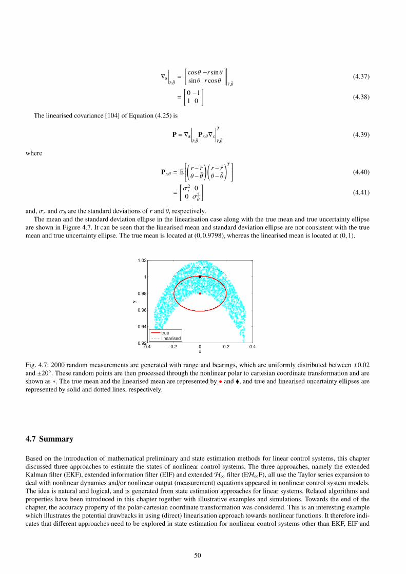
∇s
∣∣∣∣∣r,θ=
[cosθ −r sinθ
sinθ r cosθ
]∣∣∣∣∣∣r,θ
(4.37)
=
[0 −1
1 0
](4.38)
The linearised covariance [104] of Equation (4.25) is
P = ∇s
∣∣∣∣∣r,θ
Pr,θ∇s
∣∣∣∣∣T
r,θ(4.39)
where
Pr,θ = E
(
r− r
θ− θ
)(r− r
θ− θ
)T (4.40)
=
[σ2
r 0
0 σ2θ
](4.41)
and, σr and σθ are the standard deviations of r and θ, respectively.
The mean and the standard deviation ellipse in the linearisation case along with the true mean and true uncertainty ellipse
are shown in Figure 4.7. It can be seen that the linearised mean and standard deviation ellipse are not consistent with the true
mean and true uncertainty ellipse. The true mean is located at (0,0.9798), whereas the linearised mean is located at (0,1).
−0.4 −0.2 0 0.2 0.40.92
0.94
0.96
0.98
1
1.02
x
y
true
linearised
Fig. 4.7: 2000 random measurements are generated with range and bearings, which are uniformly distributed between ±0.02
and ±20. These random points are then processed through the nonlinear polar to cartesian coordinate transformation and are
shown as ∗. The true mean and the linearised mean are represented by • and , and true and linearised uncertainty ellipses are
represented by solid and dotted lines, respectively.
4.7 Summary
Based on the introduction of mathematical preliminary and state estimation methods for linear control systems, this chapter
discussed three approaches to estimate the states of nonlinear control systems. The three approaches, namely the extended
Kalman filter (EKF), extended information filter (EIF) and extendedH∞ filter (EH∞F), all use the Taylor series expansion to
deal with nonlinear dynamics and/or nonlinear output (measurement) equations appeared in nonlinear control system models.
The idea is natural and logical, and is generated from state estimation approaches for linear systems. Related algorithms and
properties have been introduced in this chapter together with illustrative examples and simulations. Towards the end of the
chapter, the accuracy property of the polar-cartesian coordinate transformation was considered. This is an interesting example
which illustrates the potential drawbacks in using (direct) linearisation approach towards nonlinear functions. It therefore indi-
cates that different approaches need to be explored in state estimation for nonlinear control systems other than EKF, EIF and
50

EH∞F introduced in this chapter in which Taylor series expansion is used. Such developments are the theme of the book and
will be discussed in the rest part of the book.
51


Chapter 5
Cubature Kalman Filter
5.1 Introductory remarks
The cubature Kalman filter (CKF) is the closest approximation known so far to the Bayesian filter that could be designed in a
nonlinear setting under the Gaussian assumption. Unlike the extended Kalman filter (EKF), CKF does not require evaluation
of Jacobians during the estimation process, while in EKF the nonlinear functions are approximated by their Jacobians, the first
order Taylor’s series approximation. The unscented Kalman filter (UKF) that is to be introduced in the last chapter is also a
useful tool in nonlinear state estimation. However, UKF performance is completely dominated by the tuning parameters, α,
β and κ. In comparison, CKF neither requires Jacobians nor depends on additional tuning parameters. CKF is therefore an
appealing option for nonlinear state estimation to EKF or UKF [5]. The idea, basic steps required in design and the properties
of CKF are to be described in this chapter.
5.2 CKF theory
Consider a nonlinear system with additive noise defined by process and measurement models in (4.1) and (4.2), listed below
for convenience,
xk = f(xk−1,uk−1)+wk−1 (5.1)
zk = h(xk,uk)+vk (5.2)
The key assumption of the cubature Kalman filter is that the predictive density p(xk|Dk−1), where Dk−1 = (ul,zl)k−1l=1
denotes
the history of input-measurement pairs up to k − 1 inclusively, and the filter likelihood density p(zk|Dk) are both Gaussian,
which eventually leads to a Gaussian posterior density p(xk|Dk). Under this assumption, the CKF solution reduces to how to
compute their means and covariances more accurately.
The CKF is a two-stage procedure comprising of prediction and update, the same as in most state estimators.
5.2.1 Prediction
At the prediction stage, the CKF computes the mean xk|k−1 of the predicted states and the associated covariance Pk|k−1 of the
Gaussian predictive density numerically using cubature rules. The predicted mean can be written as
xk|k−1 = E [f(xk−1,uk−1)+wk−1|Dk−1] (5.3)
Since wk−1 is assumed to be zero-mean and uncorrelated with the measurement sequence, it yields therefore
53

xk|k−1 = E [f(xk−1,uk−1)|Dk−1]
=
∫
Rn
f(xk−1,uk−1)p(xk−1|Dk−1)dxk−1
=
∫
Rnf(xk−1,uk−1)N(xk−1; xk−1|k−1,Pk−1|k−1)dxk−1. (5.4)
Similarly, the associated error covariance can be represented as
Pk|k−1 = E[(xk − xk|k−1)(xk − xk|k−1)T |zk−1
]
=
∫
Rn
f(xk−1,uk−1)fT (xk−1,uk−1)N(xk−1; xk−1|k−1,Pk−1|k−1)dxk−1
−xk|k−1xTk|k−1 +Qk−1. (5.5)
5.2.2 Measurement update
The predicted measurement density can be represented by
p(zk|Dk−1) =N(zk; zk|k−1,Pzz,k|k−1) (5.6)
where the predicted measurement and associated covariance are given by
zk|k−1 =
∫
Rnh(xk,uk)N(xk; xk|k−1,Pk|k−1)dxk (5.7)
Pzz,k|k−1 =
∫
Rn
h(xk,uk)hT (xk,uk)N(xk; xk|k−1,Pk|k−1)dxk − zk|k−1zTk|k−1 +Rk (5.8)
and the cross-covariance is
Pxz,k|k−1 =
∫
RnxkhT (xk,uk)N(xk; xk|k−1,Pk|k−1)dxk − xk|k−1zT
k|k−1. (5.9)
Once the new measurement zk is received, the CKF computes the posterior density p(xk|Dk) and that can be obtained as
p(xk |Dk) =N(xk; xk|k,Pk|k), (5.10)
where
xk|k = xk|k−1 +Kk(zk − zk|k−1) (5.11)
Pk|k = Pk|k−1 −KkPzz,k|k−1KTk (5.12)
with the Kalman gain given as
Kk = Pxz,k|k−1P−1zz,k|k−1 (5.13)
It can be seen that in the above prediction and measurement update equations, the Bayesian filter solution reduces to com-
puting the multi-dimensional integrals, whose integrands are all of the form nonlinear f unction×Gaussian. The heart of the
CKF is to solve (or more accurately, to approximate) the multi-dimensional integrals using cubature rules.
5.2.3 Cubature rules
The cubature rule to approximate an n-dimensional, weighted Gaussian integral is that
∫
Rnf(x)N(x;µ,P)dx ≈ 1
2n
2n∑
i=1
f(µ+P12 ξi) (5.14)
54

where P12 is a square root factor of the covariance P satisfying the relation P = P
12 (P
12 )T ; the set of 2n cubature points are given
by ξi where ξi is the i-th element of the following set
√n
1
0...
0
, . . . ,
0...
0
1
,
−1
0...
0
, . . . ,
0...
0
−1
(5.15)
These cubature rules are required to numerically evaluate the multi-integrands in the prediction and update stages of the CKF.
The cubature points required for the prediction stage are
χi,k|k−1 = P12
k−1|k−1ξi + xk−1|k−1 (5.16)
where i = 1,2, ...,2n and n is the size of the state vector.
The propagated cubature points through the process model are
χ∗i,k|k−1 = f(χi,k−1|k−1,uk−1). (5.17)
The predicted mean and error covariance matrix from (5.4), (5.5) and (5.14) are
xk|k−1 =1
2n
2n∑
i=1
χ∗i,k|k−1 (5.18)
Pk|k−1 =1
2n
2n∑
i=1
χ∗i,k|k−1χ
∗Ti,k|k−1 − xk|k−1xT
k|k−1 +Qk−1. (5.19)
By using (5.7)−(5.9) and (5.14), the predicted measurement and its associated covariances are
zk|k−1 =1
2n
2n∑
i=1
zi,k|k−1 (5.20)
Pzz,k|k−1 =1
2n
2n∑
i=1
zi,k|k−1zTi,k|k−1 − zk|k−1zT
k|k−1 +Rk (5.21)
Pxz,k|k−1 =1
2n
2n∑
i=1
χi,k|k−1zTi,k|k−1 − xk|k−1zT
k|k−1 (5.22)
where
zi,k|k−1 = h(χi,k|k−1 ,uk) (5.23)
χi,k|k−1 = P12
k|k−1ξi + xk|k−1. (5.24)
The updated state and covariance can be obtained by using Equations (5.11) and (5.13). Based on the above, the CKF can
be summarised in Algorithm 6.
5.3 Cubature transformation
Consider the polar to cartesian nonlinear transformation. The transformation can be described by
[x
y
]= h(x) =
[r cosθ
r sinθ
](5.25)
55

Algorithm 6 Cubature Kalman filter
Initialise the state vector, x0|0, and the covariance matrix, P0|0 (set k = 1).
Prediction
1: Factorise the covariance matrix, Pk−1|k−1
Pk−1|k−1 = P12
k−1|k−1P
T2
k−1,k−1
where P12
k−1|k−1is the square root factor of Pk−1|k−1.
2: Calculate the cubature points
χi,k−1|k−1 = P12
k−1|k−1ξi + xk−1|k−1, i = 1, . . . ,2n
where ξi is the i− th element of the following set
√n
1
0...
0
, . . . ,
0...
0
1
,
−1
0...
0
, . . . ,
0...
0
−1
.
3: Propagate the cubature points through the nonlinear process model
χ∗i,k−1|k−1 = f(χi,k−1|k−1,uk−1), i = 1, . . . ,2n.
4: Predicted state and covariance can be obtained as
xk|k−1 =1
2n
2n∑
i=1
χ∗i,k−1|k−1
Pk|k−1 =1
2n
2n∑
i=1
χ∗i,k−1|k−1χ
∗Ti,k−1|k−1 − xk|k−1xT
k|k−1 +Qk−1.
Measurement update
1: Factorise the predicted covariance, Pk|k−1
Pk|k−1 = P12
k|k−1P
T2
k|k−1.
2: Evaluate the cubature points (these cubature points are calculated using predicted mean and covariance, xk|k−1 and Pk|k−1)
χi,k|k−1 = P12
k|k−1ξi + xk|k−1.
3: Propagate the cubature points through the nonlinear measurement model
zi,k|k−1 = h(χi,k|k−1,uk).
4: Predicted measurement, covariance and cross-covariance can be calculated as
zk|k−1 =1
2n
2n∑
i=1
zi,k|k−1
Pzz,k|k−1 =1
2n
2n∑
i=1
zi,k|k−1zTi,k|k−1 − zk|k−1zT
k|k−1 +Rk
Pxz,k|k−1 =1
2n
2n∑
i=1
χi,k|k−1zTi,k|k−1 − xk|k−1zT
k|k−1
where the Kalman Gain is
Kk = Pxz,k|k−1P−1zz,k|k−1.
5: Update mean and error covariance can be obtained as
xk|k = xk|k−1 +Kk(zk − zTk|k−1)
Pk|k = Pk|k−1 −KkPzz,k|k−1KTk .
56
where x, consisting of polar coordinates is x = [r θ]T , and [x y]T are the cartesian coordinates, the outcome of the transfor-
mation. It is assumed that r and θ are two independent variables with means r and θ, and the corresponding standard deviations
are σr and σθ, respectively.
Consider a nonlinear function given by s = h(x) where x ∈ Rn. The mean and covariance of the random variable x are x and
Px, respectively. The mean and covariance of s, s and Ps, using cubature transformation can be calculated using Algorithm 7.
Algorithm 7 Cubature Transform
1: Compute the 2n cubature points
χi = x+P12x ξi, i = 1, . . . ,2n (5.26)
where P12 is the square root factor or P and ξi is the ith column of
√n
1
0...
0
, . . . ,
0...
0
1
,
−1
0...
0
, . . . ,
0...
0
−1
. (5.27)
The corresponding weights are
Wi =1
2n, i = 1, . . . ,2n (5.28)
2: Propagate the cubature points through the nonlinear function
si = h(χi), i = 1, . . . ,2n. (5.29)
3: The mean and covariance for s can be calculated as
s ≈2n∑
i=0
Wisi, i = 0, . . . ,2n (5.30)
Ps ≈2n∑
i=0
Wi(sisTi − ssT ), i = 0, . . . ,2n. (5.31)
5.3.1 Polar to cartesian coordinate transformation - cubature transformation
In this subsection, the polar to cartesian coordinate transformation considered in Section 4.6 will be analysed again by using
the cubature transformation. The cubature transformation given in Algorithm 7 will be used to obtain the mean and covariance
of Equation (5.25). The parameters in this subsection are the same as given in Section 4.6.
The cubature points using Equation (5.26) can be calculated as:
χ1 = x+P12x ξ1 = x+
[√nP
12x
]
1=
[1+σr
√n
π2
]
χ2 = x+P12x ξ2 = x+
[√nP
12x
]
2=
[1
π2+σθ
√n
]
χ3 = x+P12x ξ3 = x−
[√nP
12x
]
3=
[1−σr
√n
π2
]
χ4 = x+P12x ξ4 = x−
[√nP
12x
]
4=
[1
π2−σθ
√n
](5.32)
The transformed cubature points using Equation (5.29) are
57

s1 = h(χ1) = h
([1+σr
√n
π2
])=
[0
1+σr
√(n)
]
s2 = h(χ2) = h
([1
π2+σθ
√n
])=
cos
(π2+σθ
√(n)
)
sin(π2+σθ
√(n)
)
s3 = h(χ3) = h
([1
π2+σθ
√n
])=
[0
1−σr
√(n+)
]
s4 = h(χ4) = h
([1
π2−σθ
√n
])=
cos
(π2−σθ
√(n)
)
sin(π2−σθ
√(n)
) . (5.33)
-0.4 -0.2 0 0.2 0.4
x
0.92
0.94
0.96
0.98
1
1.02
y
true
linearised
cubature
Fig. 5.1: 2000 random measurements are generated with range and bearings, which are uniformly distributed between ±0.02
and ±20. These random points are then processed through the nonlinear polar to cartesian coordinate transformation and
are shown as ∗. The true-, linearised-, and cubature transformation means are represented by •, , and ⋆, respectively. True,
linearised, and cubature transformation uncertainty ellipses are represented by solid, dotted, dashed-dotted and dashed lines,
respectively.
Once the cubature points and its corresponding weights, and the transformed cubature points are obtained; the mean and
covariance of s can be calculated as
s ≈4∑
i=1
Wisi (5.34)
Ps ≈4∑
i=1
Wi(sisTi − ssT ). (5.35)
Simulations in Section 4.6 have been repeated along with cubature transformation and the corresponding results are shown
in Figure 5.1. The true mean is at (0,0.9798), the linearised mean is at (0,1), and the cubature mean is at (0,0.9798). It is very
hard to see the means of different transformations in Figure 5.1 as they are overlapped. However, by zooming in the area around
the means, they can be clearly distinguished. The uncertainty ellipse using cubature transformation is very close to the true
ellipse.
5.4 Study on a brushless DC motor
In this section a case study of a brushless DC motor (BLDC motor)is to be considered. It will show how a cubature Kalman filter
is used to estimate the unmeasurable states of the motor and the estimated states are to be fed back to the various components
of the BLDC drive to control the speed of the motor. This section first presents a detailed nonlinear model of the BLDC motor
[71]. The state vector of BLDC motor consists of currents, the speed and rotor position. The basic block diagram consists of
BLDC motor, EMF block, inverter and hysteresis block, and a PID controller is shown in Figure 5.2 [90]. The inputs to the
BLDC motor block are voltages, back EMFs and load torque and the output consists of the full state vector. The reference
58

speed and the actual speed are compared and the error between them is controlled by the PID controller, the output of the PID
controller is required to obtain the reference current, Ire f . Part of the inputs to the BLDC motor are obtained from inverter
subsystem and the other part, the back EMF, can be calculated from the EMF block. Each of these blocks is detailed in the next
few subsections.
Fig. 5.2: Block diagram of full state feedback BLDC motor.
5.4.1 BLDC motor dynamics
The state vector of BLDC motor, [ia ib ic ω θ]T , consists of phase currents, the speed and the rotor position. The phase
currents can be obtained as:
ia = i1 − i3 (5.36)
ib = i2 − i1 (5.37)
ic = i3 − i2, (5.38)
where the line-to-line currents, i1, i2 and i3, can be obtained by solving the below dynamical equations [71]:
i1 = −RLi1
(L−M)L
− eab
(L−M)L
+Vab
(L−M)L
(5.39)
i2 = −RLi2
(L−M)L
− ebc
(L−M)L
+Vbc
(L−M)L
(5.40)
i3 = −RLi3
(L−M)L
− eca
(L−M)L
+Vca
(L−M)L
, (5.41)
where RL is the line-to-line resistance, (L−M)L is the difference between the line-to-line inductance and mutual inductance;
and Vab = Va −Vb, Vbc = Vb −Vc and Vca = Vc −Va are the input voltages. In this case study, the BLDC motor parameters are
RL = 1.5Ω, (L−M)L = 6.1mH.
The line-to-line back EMFs are eab = ea−eb = Keω fab(θ), ebc = eb−ec = Keω fbc(θ) and eca = ec−ea = Keω fab(θ), where the
back EMF constant is Ke = 0.1074V/(rad/sec). The back EMFs, ea, eb and ec, as functions of the speed; and the rotor positions
are given in Table 5.1.
59

ea eb ec
0 ≤ θ < π6
6Keωπθ −Keω Keω
π6≤ θ < π
2Keω −Keω Keω
[− 6πθ+2
]
π2≤ θ < 5π
6Keω Keω
[6πθ−4
]−Keω
5π6≤ θ < 7π
6Keω
[− 6πθ+6
]Keω −Keω
7π6≤ θ < 9π
6−Keω Keω Keω
[6πθ−8
]
9π6≤ θ < 11π
6−Keω Keω
[− 6πθ+10
]Keω
11π6≤ θ ≤ 2π Keω
[6πθ−12
]Keω Keω
Table 5.1: Back EMFs as functions of θ and ω
When the stator windings are distributed, the back EMFs can also be of sinusoidal shape (as in the case of permanent
magnet synchronous motor). However, note that in this study a tetra square-wave type BLDC motor is used to demonstrate the
effectiveness of the algorithms and hence the details in Table 5.1 are given for trapezoidal waveforms. The speed and the rotor
position are:
ω =1
J[Te−TL] (5.42)
θ =P
2ω, (5.43)
where P = 6 is the number of poles and the inertia J = 8.2614×10⁻⁵kgm2, TL is the load torque and the electro-magnetic torque
Te is
Te =eaia + ebib+ ecic
ω. (5.44)
At the first instant, the above equations seem to be linear state equations, but actually they are not. This is mainly due to
the back EMFs, which involves several nonlinearities and will be discussed in Subsection 5.4.2. Further it might look like
the electro-magnetic torque (Te) will be infinity if the speed ω is zero. However, after expanding the back EMF terms (ea,
eb and ec) as given in Table 5.1, the speed in the numerator and denominator of Te are cancelled. For example, consider the
case when the 0 ≤ θ ≤ π6, ea =
6Keωπθ
,eb = −Keω,ec = Keω. Once these back EMFs are substituted in the Te expression it yields
Te =6Ke
πθia −Keib+Keic, and hence Te is independent of ω.
Note that in this book, the estimation is conducted with discrete-time models. The continuous BLDC motor model has been
discretised using the Euler’s method with sampling frequency of 10000 Hz.
5.4.2 Back EMFs and PID controller
This subsection describes the back EMFs and PID controller design.
Back EMFs
The evaluation of back EMFs plays a key role in the overall BLDC motor operation. They mainly depend on the speed and
the rotor position [71] and can be calculated using Table 5.1.
PID controller
The main aim of the PID controller is to bring the actual speed as close as to the reference speed. It is impossible to achieve
the desired performance if the PID gains are not properly tuned. In the study presented in this book, the desired closed loop
performance in terms of time domain specifications is chosen as the settling time < 1s and peak overshoot < 20%. It is possible
to choose various combinations of PID gains to achieve the desired performance. An attempt has been made to design and
implement PID controller. And, it has been found that a PI controller (with zero derivative gain) can adequately achieve the
desired performance. The Ziegler-Nichols method has been employed to find the PI controller gains, which were then manually
fine tuned to obtain the desired response. The tuned gains are, Kp = 0.05 and Ki = 10. The output of the PI controller is scaled
by Kt to obtain the reference current Ire f , which is required for the inverter subsystem to generate the desired input voltages. In
60

fab fbc fca
0 ≤ θ < π6
6θπ+1 −2 − 6θ
π+1
π6≤ θ < π
22 6θ
π−5 3− 6θ
ππ2≤ θ < 5π
6− 6θ
π+5 6θ
π−3 −2
5π6≤ θ < 7π
6− 6θ
π+5 2 6θ
π−7
7π6≤ θ < 9π
6−2 − 6θ
π+9 6θ
π−7
9π6≤ θ < 11π
66θπ−11 − 6θ
π+9 2
11π6≤ θ ≤ 2π 6θ
π−11 −2 13− 6θ
π
Table 5.2: The functions fab, fbc and fca
this study the torque constant is assumed to be Kt = 0.21476Nm.
Inverter and hysteresis block
The inverter subsystem is responsible to generate the required voltages for the BLDC motor based on the hysteresis current
control. The hysteresis current control provides the switching functions which are required to calculate the phase and line-to-
line voltages. The switching functions can be obtained using Table 5.3, where Iad, Ibd and Icd are the delayed phase currents
[71], and T1 and T2 depends on the corresponding current sequence.
For example, consider the case of current ia. When ia is positive
T1 =
[(ia < 0.9Ire f )− (ia > 1.1Ire f )+ (ia > 0.9Ire f )× (ia < 1.1Ire f )× (ia > iad)
−(ia > 0.9Ire f )× (ia < 1.1Ire f )× (ia < iad)
](5.45)
The functioning of T1 is based on the ia, Ire f and the previous sample current iad. Suppose if (ia < 0.9Ire f ) i.e. the first term of
the above equation is satisfied (and hence the other three terms are zero), will give T1 = 1. Similarly, if ia > 1.1Ire f , the second
term will be activated, which will give T1 = −1. If 0.9Ire f < ia < 1.1Ire f and ia > iad then the third term will be activated, which
will make T = 1. Finally, if 0.9Ire f < ia < 1.1Ire f and ia < iad, then fourth term will be activated to yield T1 = −1.
When ia is negative,
T2 =
[− (ia > −0.9Ire f )+ (ia < −1.1Ire f )− (ia < −0.9Ire f )(ia > −1.1Ire f )× (ia < iad)
+(ia < −0.9Ire f )× (ia > −1.1Ire f )× (ia > iad)
]. (5.46)
The lower and upper limits of hysteresis current controller are given by 0.9Ire f and 1.1Ire f , respectively. Similarly, for the
other currents ib and ic, the corresponding T1 and T2 can be calculated.
Inputs Outputs
Ia, Iad Fa = (θ > π/6)(θ < 5π/6)T1+ (θ > 7π/6)(θ < 11π/6)T2
Ib, Ibd Fb = (θ > 0)(θ < π/2)T2+ (θ > 5π/6)(θ < 9π/6)T1
+(θ > 11π/6)(θ < 2π)T2
Ic, Icd Fc = (θ > 0)(θ < π/6)T1+ (θ > π/2)(θ < 7π/6)T2
+(θ > 9π/6)(θ < 2π)T1
Table 5.3: Switching functions for hysteresis current control
Based on these switching functions, the phase voltages can be calculated as:
Va =Vd
2Fa
Vb =Vd
2Fb
Vc =Vd
2Fc, (5.47)
61

where, Vd is the DC link voltage and can be obtained either by pre-design analysis or by using a suitable rectifier. The inverter
line-to-line voltages can now be obtained as
Vab = Va−Vb
Vbc = Vb−Vc
Vca = Vc−Va. (5.48)
These line-to-line voltages are the inputs to the BLDC motor.
Fig. 5.3: Proposed scheme for a BLDC motor.
Finally, the state vector and output of BLDC motor model can be expressed in the state-space form as:
x = F(x)x + Gd + VTL
iaibicω
θ
=
− RL
(L−M)L0 0 − Ke
(L−M)Lfab(θ) 0
0 − RL
(L−M)L0 − Ke
(L−M)Lfbc(θ) 0
0 0 − RL
(L−M)L− Ke
(L−M)Lfca(θ) 0
Ke
Jfab(θ)
Ke
Jfbc(θ)
Ke
Jfca(θ) − B
J0
0 0 0 P2
0
iaibicω
θ
+
1(L−M)L
0 0
0 1(L−M)L
0
0 0 1(L−M)L
0 0 0
0 0 0
Vab
Vbc
Vca
+
0
0
01J
0
TL (5.49)
The output equation is:
y = Hx
=
1 0 0 0 0
0 1 0 0 0
0 0 1 0 0
iaibicω
θ
(5.50)
The process and measurement noises are added to the state and output equations, respectively. The equations in (5.49) and
(5.50) are in the continuous-time domain, however the estimation methods implemented are in the discrete-time domain. Hence
62

these equations have been discretised by using Euler’s method1 such that:
xn+1 = (I5 +F(xn)∆t)xn+G∆td+V∆tTL (5.51)
where I5 is the fifth order identity matrix and ∆t is the sampling time. The output equation in the discrete-time domain will be
the same as the one given in (5.50), that is
yn = Hxn. (5.52)
The following assumptions have been considered for the mathematical model of the BLDC motor and power converters.
The magnetic flux in the motor stator winding is not saturated; stator resistances of all three phase windings are equal; self and
mutual inductances are constant and they are not varying with load variation; devices in the inverter are idea and iron losses are
negligible [68].
Note that, since the back EMF of a BLDC motor is of trapezoidal shape, the BLDC motor is controlled by exciting only
two phases at a time for every 60 degrees of rotor position. Further, one can calculate all the three currents by using only two
current sensors as
ia + ib+ ic = 0.
Due to the sensor noise in the current sensors, it is not always possible to accurately calculate all the three currents from two
current sensors. Specifically, during the low speed operations the current sensors used in this study have a low signal-to-noise
ratio. Hence, three current sensors are used for the efficient control of the BLDC motor (whereas only two phases are excited at
a time). However, by using only two high resolution current sensors one can control the BLDC motor efficiently as well.
5.4.3 Initialisation of the state estimators
In the implementation it is required first to initialise the state vector (five states in all) and the corresponding covariance matrix,
and then to choose appropriate process and noise covariance matrices Qn and Rn. The initial state vector x0 and covariance
matrix P0 are randomly selected fromN([0 0 0 0.01 0.01]T ,10−5I5), whereN represents the normal-distributed random
variables. The process noise covariance Qn is a fifth order diagonal matrix with all the diagonal elements as 10−12 and the
measurement noise covariance Rn is a third order diagonal matrix with all the diagonal elements as 0.01. With the initial values
and the plant dynamic model, Algorithm 6 and Algorithm 3 can be implemented.
5.4.4 BLDC motor experiments
This subsection describes the setup of a BLDC motor system and shows the experimental results using the cubature Kalman
filter (CKF) compared with that from the extended Kalman filter (EKF).
Experiment setup
The setup consists of a BLDC motor system with incremental encoder, intelligent power module [2] (including rectifier,
input filter using capacitors, dynamic braking module, voltage source inverter, gate driver circuit and optocoupler), current
sensors (LTS 25 NP current transducers), dSPACE DS1103 controller board, dSPACE CLP1103 connector panel [1] and a
desk-top computer (dSPACEcontrol desk). These devices are interconnected as shown in Figure 5.4 and depicted in the block
diagram Figure 5.5.
The measured currents are processed through the dSPACE CLP1103 connector panel which has analog-to-digital and digital-
to-analog ports and a provision to give inputs to the dSPACE DS1103 board. The dSPACE DS1103 controller board has a DSP
processor which has analog-to-digital and digital-to-analog converters and other components required for the data processing.
Several filters are also included for signal conditioning purposes. The block diagram given in Figure 5.6 is simulated using the
various dSPACE compatible RTI and Simulink blocksets in the computer. This Simulink diagram is then converted to a set
1 The continuous state-space model, x = Ax+Bu, can be discretised by using Euler’s method as
xn+1 = (In +A∆t)xn +∆tBu,
where ∆t is the sampling time and In is the nth order identity matrix
63

(a) Front view of the experimental setup for BLDC drive. (b) Side view of the experimental BLDC drive.
Fig. 5.4: Experimental setup for BLDC drive
Fig. 5.5: Block diagram for BLDC drive experiment.
Fig. 5.6: Speed controller scheme using CKF.
64
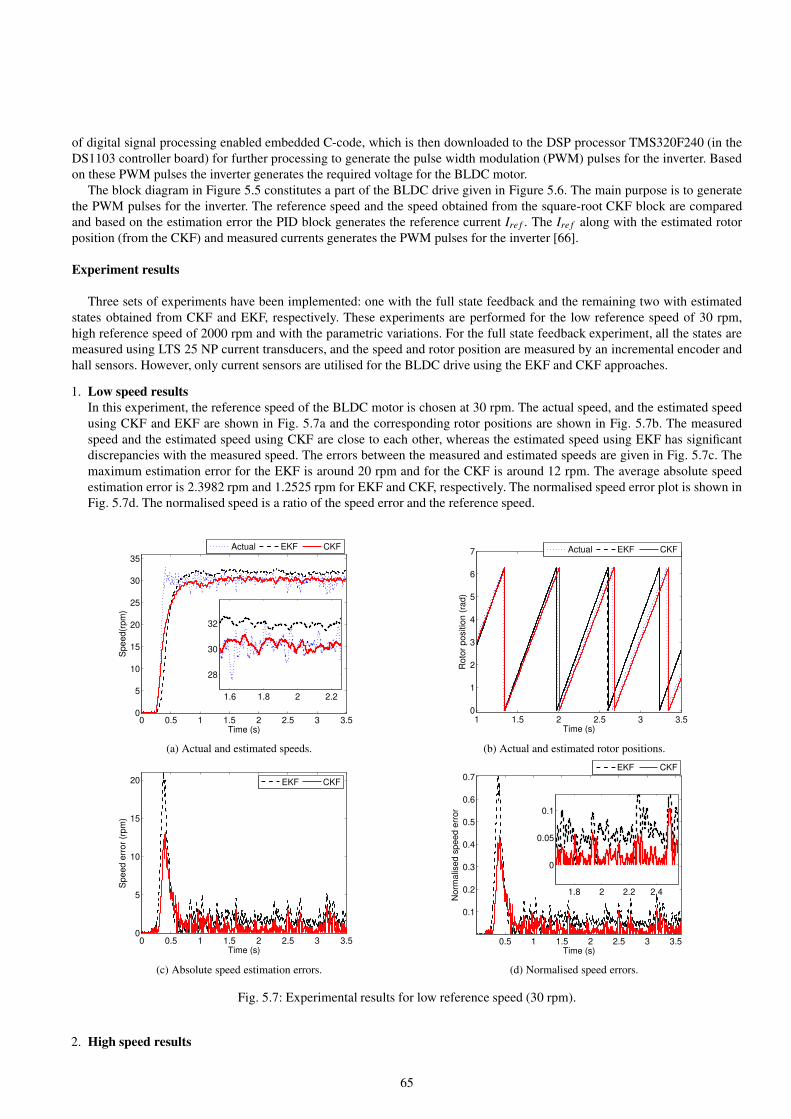
of digital signal processing enabled embedded C-code, which is then downloaded to the DSP processor TMS320F240 (in the
DS1103 controller board) for further processing to generate the pulse width modulation (PWM) pulses for the inverter. Based
on these PWM pulses the inverter generates the required voltage for the BLDC motor.
The block diagram in Figure 5.5 constitutes a part of the BLDC drive given in Figure 5.6. The main purpose is to generate
the PWM pulses for the inverter. The reference speed and the speed obtained from the square-root CKF block are compared
and based on the estimation error the PID block generates the reference current Ire f . The Ire f along with the estimated rotor
position (from the CKF) and measured currents generates the PWM pulses for the inverter [66].
Experiment results
Three sets of experiments have been implemented: one with the full state feedback and the remaining two with estimated
states obtained from CKF and EKF, respectively. These experiments are performed for the low reference speed of 30 rpm,
high reference speed of 2000 rpm and with the parametric variations. For the full state feedback experiment, all the states are
measured using LTS 25 NP current transducers, and the speed and rotor position are measured by an incremental encoder and
hall sensors. However, only current sensors are utilised for the BLDC drive using the EKF and CKF approaches.
1. Low speed results
In this experiment, the reference speed of the BLDC motor is chosen at 30 rpm. The actual speed, and the estimated speed
using CKF and EKF are shown in Fig. 5.7a and the corresponding rotor positions are shown in Fig. 5.7b. The measured
speed and the estimated speed using CKF are close to each other, whereas the estimated speed using EKF has significant
discrepancies with the measured speed. The errors between the measured and estimated speeds are given in Fig. 5.7c. The
maximum estimation error for the EKF is around 20 rpm and for the CKF is around 12 rpm. The average absolute speed
estimation error is 2.3982 rpm and 1.2525 rpm for EKF and CKF, respectively. The normalised speed error plot is shown in
Fig. 5.7d. The normalised speed is a ratio of the speed error and the reference speed.
0 0.5 1 1.5 2 2.5 3 3.50
5
10
15
20
25
30
35
Time (s)
Sp
ee
d(r
pm
)
Actual EKF CKF
1.6 1.8 2 2.2
28
30
32
(a) Actual and estimated speeds.
1 1.5 2 2.5 3 3.50
1
2
3
4
5
6
7
Time (s)
Ro
tor
po
sitio
n (
rad
)
Actual EKF CKF
(b) Actual and estimated rotor positions.
0 0.5 1 1.5 2 2.5 3 3.50
5
10
15
20
Time (s)
Sp
ee
d e
rro
r (r
pm
)
EKF CKF
(c) Absolute speed estimation errors.
0.5 1 1.5 2 2.5 3 3.5
0.1
0.2
0.3
0.4
0.5
0.6
0.7
Time (s)
No
rma
lise
d s
pe
ed
err
or
EKF CKF
1.8 2 2.2 2.4
0
0.05
0.1
(d) Normalised speed errors.
Fig. 5.7: Experimental results for low reference speed (30 rpm).
2. High speed results
65

In this experiment, the reference speed of the BLDC motor is chosen as a ramp signal (slope of 400 rpm/s) with the final value
of 2000 rpm. The actual speed, and the estimated speed using EKF and CKF are shown in Fig. 5.8a and the corresponding
rotor positions are shown in Fig. 5.8b. Similar to the low speed simulations, the measured speed and the estimated speed
using CKF are close to each other, whereas the estimated speed using EKF has significant errors. The errors between the
measured and estimated speeds are given in Fig. 5.8c. The maximum estimation error for the EKF is around 115 rpm and
for the CKF is around 40 rpm. The average absolute speed estimation error is 25.8198 rpm and 13.1036 rpm for EKF and
CKF, respectively. The normalised speed error plot is shown in Fig. 5.8d.
0 2 4 6 8 100
500
1000
1500
2000
2500
Time (s)
Sp
ee
d(r
pm
)
Actual EKF CKF
6.5 7 7.51950
2000
2050
2100
(a) Actual and estimated speeds.
9.9 9.92 9.94 9.96 9.98 100
1
2
3
4
5
6
7
Time (s)
Ro
tor
po
sitio
n (
rad
)
Actual EKF CKF
(b) Actual and estimated rotor positions.
0 2 4 6 8 100
20
40
60
80
100
120
Time (s)
Sp
ee
d E
rro
r(rp
m)
EKF CKF
(c) Absolute speed estimation errors.
0 2 4 6 8 100
0.01
0.02
0.03
0.04
0.05
0.06
0.07
Time (s)
No
rma
lise
d s
pe
ed
err
or
EKF CKF
(d) Normalised speed errors.
Fig. 5.8: Experimental results for high reference speed (2000 rpm).
3. Robustness analysis
In this part, the performance of the estimators in the presence of various uncertainties is considered. These experiments are
performed at the low reference speed of 30 rpm and the steady state results are analysed.
Load torque variation
In this experiment, the load torques of 2 N-m and 4 N-m are considered. These mechanical loads are applied from the starting
of the experiment. The nominal results (without load torque variation) are given in Fig. 5.9a, the absolute average speed error
is 1.7327 rpm and 0.7967 rpm for EKF and CKF, respectively. The speed errors with the load torque of 2 N-m are given
in Fig. 5.9b, where the absolute average errors are 1.1968 rpm and 0.8336 rpm for EKF and CKF, respectively. The speed
errors with the load torque of 4 N-m are given in Fig. 5.9c, where the average errors for EKF and CKF are 2.4086 rpm and
1.1743 rpm, respectively.
Stator resistance variation
In this experiment, the stator resistances for the estimators are varied +/−30% from the nominal value. The nominal results
(without the stator resistance variation) are the same as seen in Fig. 5.9a. The speed errors with +30% variation of the stator
resistance from its nominal value are given in Fig. 5.10a, where the absolute average errors are 1.9144 rpm and 0.9866 rpm
for EKF and CKF, respectively. The speed errors with −30% variation of stator resistance from its nominal value are given
66
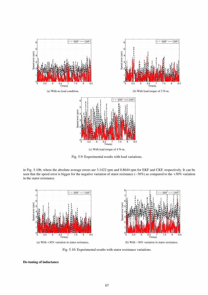
5 5.5 6 6.5 7 7.5 8 8.50
1
2
3
4
5
6
Time(s)
Sp
ee
d e
rro
r (r
pm
)
EKF CKF
(a) With no load condition.
5 5.5 6 6.5 7 7.5 8 8.50
1
2
3
4
5
6
Time(s)
Sp
ee
d e
rro
r (r
pm
)
EKF CKF
(b) With load torque of 2 N-m.
5 5.5 6 6.5 7 7.5 8 8.50
1
2
3
4
5
6
Time(s)
Sp
ee
d e
rro
r (r
pm
)
EKF CKF
(c) With load torque of 4 N-m.
Fig. 5.9: Experimental results with load variations.
in Fig. 5.10b, where the absolute average errors are 3.1422 rpm and 0.8644 rpm for EKF and CKF, respectively. It can be
seen that the speed error is bigger for the negative variation of stator resistance (−30%) as compared to the +30% variation
in the stator resistance.
5 5.5 6 6.5 7 7.5 8 8.50
1
2
3
4
5
6
7
8
Time(s)
Sp
ee
d e
rro
r (r
pm
)
EKF CKF
(a) With +30% variation in stator resistance.
5 5.5 6 6.5 7 7.5 8 8.50
1
2
3
4
5
6
7
8
Time(s)
Sp
ee
d e
rro
r (r
pm
)
EKF CKF
(b) With −30% variation in stator resistance.
Fig. 5.10: Experimental results with stator resistance variations.
De-tuning of inductance
67

In this experiment, the stator inductance for the estimators is de-tuned by 10% from its nominal value. The nominal results
(without de-tuning) are the same as given in Fig. 5.9a. The results with de-tuned inductance are given in Fig. 5.11, where
the absolute average speed errors are 3.5140 rpm and 1.8106 rpm for the cases of EKF and CKF, respectively.
5 5.5 6 6.5 7 7.5 8 8.50
1
2
3
4
5
6
7
8
Time(s)
Sp
ee
d e
rro
r (r
pm
)
EKF CKF
Fig. 5.11: Estimation errors with de-tuned stator inductance.
The experimental results shown above demonstrate that it is possible to estimate the speed and rotor positions with either
EKF or CKF. The experiments with different parametric variations show the robustness property of the EKF and CKF. However
in all the cases the performance of the CKF is better than that of the EKF approach. That is due to the fact that EKF is based
on the first order approximation of the nonlinear function, whereas this approximation is not required for the CKF. Further, the
calculation of the Jacobians for the EKF are quite complex and in some cases there is a possibility that these Jacobians can
become singular leading to numerical instability. It can also be observed that among the considered uncertainties, the estimator
performance is sensitive to the de-tuned inductance.
5.5 Summary
In this chapter the cubature Kalman filter (CKF) has been introduced. CKF does not use the Taylor series expansion of nonlinear
functions involved in the system equations, which is obviously a great advantage in state estimation for nonlinear systems. CKF
is also the closest known approximation to the Bayesian filter that could be designed under the Gaussian assumption. Follow-
ing the introduction of CKF algorithm and relevant calculation approaches, the polar to cartesian coordinates transformation
example was considered again. The cubature transformation that is the basis of CKF was applied this time in the coordinates
transformation. It is shown that with regard to the means and standard deviation ellipses, the cubature transform outperforms
the linearisation approach for nonlinear functions using the Taylor series expansion.
Further to illustrate the use of nonlinear state estimation approaches, a case of brushless DC motor control system was studied
in this chapter. A laboratory experimental setup was introduced and both the extended Kalman filter (EKF) and cubature Kalman
filter (EKF) were explored in the state estimation combined with a state feedback control scheme. Experimental results showed
some advantages of using the CKF approach over the EKF approach in such applications.
68

Chapter 6
Variants of Cubature Kalman Filter
6.1 Introductory remarks
Cubature Kalman filter (CKF) discussed in the last chapter deals with nonlinear systems with single set of sensors and with
Gaussian noise. In this chapter, variants of CKF, namely the cubature information filter (CIF), cubature H∞ filter (CH∞F)
and cubatureH∞ information filter (CH∞IF), and their square-root versions, will be explored. Each of these filters is suitable
for particular applications. For example, the CIF is suitable for state estimation of nonlinear systems with multiple sensors
in the presence of Gaussian noise; the CH∞F is suitable for nonlinear systems with Gaussian or non-Gaussian noises; and
finally, the CH∞IF is useful for estimating the states of nonlinear systems with multiple sensors in the presence of Gaussian or
non-Gaussian noise.
6.2 Cubature information filters
Similar to the Kalman filter, an information filter (IF) is also formed by two stages - prediction and update. A Kalman in-
formation filter is an algebraic equivalent of a Kalman filter where the information vector and information matrices (inverse
of covariance matrices) are propagated instead of mean and covariances in the Kalman filter algorithm. Initialisation in the
information space is easier (or, more tolerant) than in the Kalman filter case and the update stage of an information filter is
computationally simpler than that in the Kalman filter. The information filter for linear systems and the extended information
filter for nonlinear systems were introduced earlier in Chapter 3 and Chapter 4, respectively. For the sake of convenience, they
are repeated here with only the main ingredients of each of them, before the cubature information filter is discussed. One may
see [18] for more details.
6.2.1 Information filters
Consider the discrete, linear process and measurement models depicted in the following
xk = Fk−1xk−1 +Gk−1uk−1 +wk−1, (6.1)
zk = Hkxk +vk, (6.2)
where k ≥ 1 is the time index, xk the state vector, uk the control input, zk the measurement, wk−1 and vk are the process and
measurement noises, respectively.
The predicted information state vector, yk|k−1, and the predicted information matrix, Yk|k−1, are defined as
yk|k−1 = Yk|k−1xk|k−1 (6.3)
Yk|k−1 = P−1k|k−1 =
[Fk−1Y−1
k−1|k−1FTk−1 +Qk−1
]−1(6.4)
where Pk|k−1 is the predicted covariance matrix and
xk|k−1 = Fk−1xk−1|k−1 +Gk−1uk−1. (6.5)
69

The updated information state vector, yk|k, and the updated information matrix, Yk|k, are
yk|k = yk|k−1 + ik (6.6)
Yk|k = Yk|k−1 + Ik. (6.7)
The information state contribution, ik, and its associated information matrix, Ik, are
ik = HTk R−1
k zk (6.8)
Ik = HTk R−1
k Hk (6.9)
Recovery of state vector and covariance matrix is required at different stages and can be conducted, for example, by using
MATLAB’s leftdivide operator [36],
xk|k = Yk|k\yk|k (6.10)
Pk|k = Yk|k\In (6.11)
where In is the identity matrix of dimension n, with n being the size of the state vector.
6.2.2 Extended information filter
The extended information filter was introduced in Chapter 4. For the convenience of reference, the main formulae are repeated
here. For detailed formulations and derivations of these filtering algorithms, please see Chapter 4 or [83] for example.
Similar to the information filter, the extended information filter is interested to find out the value of the information states
and the value of the information matrix which is the inverse of the covariance matrix. However, EIF can be applied for nonlinear
systems, that is not possible for the (standard) information filter. The EIF equations are to be listed below.
Consider the discrete-time, nonlinear process and measurement models as
xk = f(xk−1,uk−1)+wk−1 (6.12)
zk = h(xk,uk)+vk (6.13)
where k is the time index, xk the state vector, uk the control input, zk the measurement, wk−1 and vk are the process and
measurement noises, respectively. These noises are assumed to be zero mean, Gaussian-distributed, random variables with
covariances of Qk−1 and Rk, respectively.
The predicted information state vector, yk|k−1, and the predicted information matrix, Yk|k−1, can be calculated by
yk|k−1 = Yk|k−1xk|k−1 (6.14)
Yk|k−1 = P−1k|k−1 =
[∇fxY−1
k−1|k−1∇fTx +Qk−1
]−1(6.15)
where Pk|k−1 is the predicted covariance matrix and
xk|k−1 = f(xk−1|k−1,uk−1). (6.16)
The updated information state vector, yk|k, and the updated information matrix, Yk|k, are
yk|k = yk|k−1 + ik (6.17)
Yk|k = Yk|k−1 + Ik. (6.18)
The information state contribution, ik, and its associated information matrix contribution, Ik, are
ik = ∇hTx R−1
k
[νk +∇hxxk|k−1
](6.19)
Ik = ∇hTx R−1
k ∇hx (6.20)
where the measurement residual, νk, is
νk = zk −h(xk|k−1,uk) (6.21)
70

and ∇fx, and ∇hx are the Jacobians of f and h evaluated at the best available state, respectively.
For the nonlinear information filter, recovery of state and covariance matrices is required at different stages. As in the
information filter design for linear systems, the state vector and covariance matrix can be recovered by
xk|k = Yk|k\yk|k (6.22)
Pk|k = Yk|k\In (6.23)
where In is the identity matrix of dimension n, the dimension of the state vector.
6.2.3 Cubature information filter
This section presents the cubature information filter (CIF) algorithm, which explores the CKF in an EIF framework. The
factorisation of the error covariance matrix, Pk−1|k−1, is given by,
Pk−1|k−1 = P12
k−1|k−1P
T2
k−1,k−1
where P12
k−1|k−1is the square root factor of Pk−1|k−1, the evaluation of cubature points and propagated cubature points for the
process model, as required for cubature Kalman filtering process, are shown in (6.24)−(6.25).
Let the information state vector and information matrix be given by ˆyk−1|k−1 and[Yk−1|k−1
], respectively, and let Sk−1|k−1 be
a square root factor of[Yk−1|k−1
]−1.
The evaluation of the cubature points and propagated cubature points can then be given as
χi,k−1|k−1 = Sk−1|k−1ξi + xk−1|k−1 (6.24)
χ∗i,k|k−1 = f(χi,k−1|k−1,uk−1) (6.25)
where i = 1,2, ...,2n and n is the size of the state vector.
From (6.57) and (5.19), and (6.57) and (5.18), it yields
Yk|k−1 = P−1k|k−1
=
1
2n
2n∑
i=1
χ∗i,k|k−1χ
∗Ti,k|k−1 − xk|k−1xT
k|k−1 +Qk−1
−1
(6.26)
and
yk|k−1 = P−1k|k−1xk|k−1 (6.27)
= Yk|k−1xk|k−1 (6.28)
=1
2n
Yk|k−1
2n∑
i=1
χ∗i,k|k−1
. (6.29)
In the measurement update stage of the CIF, the first two steps involve the evaluation of propagated cubature points and the
predicted measurement is given below. The propagated cubature points for the measurement model can be evaluated as
χi,k|k−1 = Sk|k−1ξi + xk|k−1 (6.30)
zi,k|k−1 = h(χi,k|k−1,uk). (6.31)
The predicted measurement is
zk|k−1 =1
2n
2n∑
i=1
zi,k|k−1. (6.32)
71

The information state contribution and its associated information matrix contribution in (6.19) and (6.20) are explicit func-
tions of the linearised Jacobian of the measurement model. But the CKF algorithm does not require the Jacobians for mea-
surement update and hence it cannot be directly used in the EIF framework. However, by using the following linear error
propagation property [72], [103], it is possible to embed the CKF update in the EIF framework. The linear error propagation
property for the error cross covariance matrix can be approximated as [103]
Pxz,k|k−1 ≃ Pk|k−1∇hTx . (6.33)
By multiplying P−1k|k−1
and Pk|k−1 on the RHS of (6.19) and (6.20) we get
ik = P−1k|k−1Pk|k−1∇hT
x R−1k
[νk +∇hxPT
k|k−1P−Tk|k−1xk|k−1
](6.34)
Ik = P−1k|k−1Pk|k−1∇hT
x R−1k ∇hxPT
k|k−1P−Tk|k−1. (6.35)
Using (6.33) in (6.34) and (6.35) we get
ik = P−1k|k−1Pxz,k|k−1R−1
k
[νk +PT
xz,k|k−1P−Tk|k−1xk|k−1
](6.36)
Ik = P−1k|k−1Pxz,k|k−1R−1
k PTxz,k|k−1P−T
k|k−1 (6.37)
where
Pxz,k|k−1 =1
2n
2n∑
i=1
χi,k|k−1zTi,k|k−1 − xk|k−1zT
k|k−1. (6.38)
The updated information state vector and information matrix for the CIF can be obtained by using ik and Ik from (6.36) and
(6.37) in (6.17) and (6.18).
One may note that, unlike in the case of the information filter for linear systems, zero initialisation is not possible in a
cubature information filter. That is because the evaluation of cubature points requires the square root of the covariance matrix.
The state vector and covariance matrix in the cubature information filtering process can be recovered by (6.22) and (6.23). The
CIF algorithm is summarised in Algorithm 8.
6.2.4 CIF in multi-sensor state estimation
One of the main advantages of an information filter is its ability to deal with multi-sensor data fusion [11, 83]. The information
from various sensors can be easily fused by simply adding the information contributions to the information matrix and informa-
tion vector [11, 83]. In the multi-sensor state estimation, the available observations consist of measurements taken from various
sensors. The prediction step for the multi-sensor state estimation is similar to that of the Kalman or (single sensor) information
filters. In the measurement update step, the data from various sensors are fused together for an efficient and reliable estimation
[93].
Let the various sensors used for state estimation be given by
z j,k = h j,k(xk,uk)+v j,k; j = 1,2, ...D (6.39)
where ‘D’ is the number of sensors.
The CIF algorithm can be easily extended for the multi-sensor data fusion in which the basic update step of CIF is similar
to EIF [83]. The updated information vector and information matrix for multi-sensor CIF are
yk|k = yk|k−1 +
D∑
j=1
i j,k (6.40)
Yk|k = Yk|k−1 +
D∑
j=1
I j,k. (6.41)
By using (6.36) and (6.37), the information contributions of multi-sensor CIF are
72

I j,k = MTj,k|k−1R−1
j,kM j,k|k−1 (6.42)
i j,k = MTj,k|k−1R−1
j,k [ν j,k +M j,k|k−1xk|k−1] (6.43)
where
MTj,k|k−1 = P−1
k|k−1P j,xz,k|k−1 . (6.44)
73

Algorithm 8 Cubature information filter
Prediction
1: Evaluate χi,k−1|k−1, χ∗i,k|k−1
and xk|k−1 as
χi,k−1|k−1 =
√Yk−1|k−1\Inξi + (Yk−1|k−1\yk−1|k−1),
χ∗i,k|k−1 = f(χi,k−1|k−1,uk−1)
xk|k−1 =1
2n
2n∑
i=1
χ∗i,k|k−1
where ‘\’ is left-divide operator, In is the nth order identity matrix, and ξi is the i-th element of the following set
√n
1
0...
0
, . . . ,
0...
0
1
,
−1
0...
0
, . . . ,
0...
0
−1
(6.45)
.
2: The predicted information matrix and information vector are:
Yk|k−1 = P−1k|k−1
yk|k−1 = Yk|k−11
2n
2n∑
i=1
χ∗i,k−1|k−1
where
Pk|k−1 =1
2n
2n∑
i=1
χ∗i,k|k−1χ
∗Ti,k|k−1 − xk|k−1xT
k|k−1 +Qk−1
Measurement Update
1: Evaluate the information state contribution and its associated information matrix contribution as
Ik =Yk|k−1Pxz,k|k−1R−1k PT
xz,k|k−1YTk|k−1
ik =Yk|k−1Pxz,k|k−1R−1k
[νk +PT
xz,k|k−1YTk|k−1xk|k−1
]
where
Pxz,k|k−1 =1
2n
2n∑
i=1
χi,k|k−1zTi,k|k−1 − xk|k−1zT
k|k−1.
2: The estimated information vector and information matrix of CIF are
Yk|k = Yk|k−1 + Ik
yk|k = yk|k−1 + ik.
The state and covariance can be recovered using (6.22) and (6.23).
74

6.3 Cubature H∞ filters
The H∞ filter, the extended H∞ filter (EH∞F) and the extended information filter were introduced in Chapter 3 and Chapter
4, respectively. Again, the concept and main steps of those filtering approaches will be briefly summarised here for the sake of
convenience. Based on these filters, the extendedH∞ information filter (EH∞IF) will be introduced in this section before the
introduction of the cubatureH∞ filter (CH∞F) and cubatureH∞ information filter (CH∞IF).
6.3.1 H∞ filters
For a general nonlinear system, the discrete-time model can be given as
xk = f[xk−1,uk−1]+wk−1 (6.46)
zk = h[xk,uk]+vk (6.47)
where k is the time index showing the current time, xk ∈ Rn is the state vector, uk ∈ Rq the control input, zk ∈Rp the measurement
vector, and wk−1 and vk are the process and observation noises, respectively.
A solution to the H∞ filter based on the game theory was given in [100]. Consider the process and observation models
defined in (6.46) and (6.47). The noise terms wk and vk may be random with possibly unknown statistics, or they may be
deterministic. Also, they may have zero or nonzero means. Instead of directly estimating the states, one can estimate a linear
combination of the states
zk = Lkxk (6.48)
By replacing L with the identity matrix of appropriate size, it returns to the normal scenario of estimation of the state vector.
In the game theory approach to theH∞ filtering, the performance measure is given by
J∞ =
∑N−1k=0‖zk − zk‖2Mk
‖x0 − x0‖2P−1
0
+∑N−1
k=0(‖wk‖2
Q−1k
+ ‖vk‖2R−1
k
)(6.49)
where P0, Qk, Rk, and Mk are symmetric, positive definite, weighing matrices chosen by the user based on the problem at hand.
The norm notation used in this section is ‖e‖2S k= eT S ke.
The H∞ filter is designed to minimise the state estimation error so that J∞ is bounded by a prescribed threshold under the
“worst” possible case of wk, vk, and x0
supJ∞ < γ2 (6.50)
where “sup” stands for supremum, and γ > 0 is the error attenuation parameter.
Based on (6.50), the designer should find xk so that J∞ < γ2 holds for any possible values in wk, vk, and x0. The best that the
designer can do is to minimise J∞ under worst case scenarios, then theH∞ filter can be interpreted as the following ‘minimax’
problem
min max J∞xk wk ,vk ,x0
(6.51)
The predicted state vector and auxiliary matrix are
xk|k−1 = f(xk−1|k−1,uk−1) (6.52)
Pk|k−1 = ∇fxPk−1|k−1∇fTx +Qk (6.53)
and the inverse of the updated auxiliary matrix can be obtained as
P−1k|k = P−1
k|k−1 +∇hTx R−1
k ∇hx −γ−2In (6.54)
75

where In denotes the identity matrix of dimension n×n.
The updated state is
xk|k = xk|k−1 +K∞[zk −h(xk|k−1)] (6.55)
where
K∞ = Pk|k−1∇hTx [∇hxPk|k−1∇hT
x +Rk]−1 (6.56)
The Jacobians of f and h, ∇fx and ∇hx, are evaluated at xk−1|k−1 and xk|k−1, respectively.
6.3.2 ExtendedH∞ information filter
It is required first to initialise the information vector and information matrix, I0|0 and s0|0, for k = 1. The extendedH∞ infor-
mation filter (EH∞IF) procedure can then be described below.
Prediction stage in the EH∞IF:
The predicted information matrix (the inverse of the predicted covariance matrix) and the corresponding information vector
are
Ik|k−1 =[∇fI−1
k−1|k−1∇fT +Qk−1
]−1(6.57)
sk|k−1 = Ik|k−1xk|k−1 (6.58)
where
xk|k−1 = f(Ik|k−1k−1|k−1\sk−1|k−1,uk−1).
Note that the prediction step for the EH∞IF is the same as that of the one given in the EIF in Section 4.3, except that Qk−1
and Rk are the weighting matrices rather than noise covariances. The update stage, where the sensor measurements are required,
will however be different from the traditional EH∞F or EIF given in Sections 3.4 and 4.3.
Update stage in the EH∞IF:
The updated information vector and information matrix are
sk|k = sk|k−1 + ik (6.59)
Ik|k = Ik|k−1 + Ik. (6.60)
where
ik = ∇hT R−1k
[νk +∇hxk|k−1
](6.61)
Ik = ∇hT R−1k ∇h−γ−2
In (6.62)
and
νk = zk −h(xk|k−1,uk). (6.63)
Note that the main difference between the update stages of the EIF and the EH∞IF is in the information matrix contribution
Ik.
For multi-sensor state estimations, the measurement comes from various sensors and can be fused to estimate the state vector
efficiently in the following way
76
sk|k = sk|k−1 +
D∑
j=1
i j,k (6.64)
Ik|k = Ik|k−1 +
D∑
j=1
I j,k, (6.65)
where
i j,k = ∇hTj,k|k−1R−1
j,k [ν j,k +∇hTj,k|k−1xk|k−1] (6.66)
I j,k = ∇hTj,k|k−1R−1
j,k∇hTj,k|k−1 −γ−2
In (6.67)
(6.68)
and ∇hTj,k|k−1
represents the Jacobian of the nonlinear measurement function h j,k|k−1 of the ‘ jth’ sensor channel, and R j,k is the
corresponding noise.
6.3.3 CubatureH∞ filter
It can be seen from Section 3.4 that EH∞F requires Jacobians, and the CKF discussed in Section 5.2 assumes that the statistical
noise properties are known during the state estimation. In this subsection, we present a nonlinear estimation algorithm, the
cubature H∞ filter (CH∞F), in which neither the Jacobians nor the statistical noise properties are used a priori for the state
estimation. This approach can be useful in the presence of parametric uncertainties, too. Furthermore, if some of the statistical
properties of noises are known a priori, then it can be incorporated in the proposed method. In the cubatureH∞ filter algorithm,
the prediction step is similar to that of CKF, which involves the factorisation of the error auxiliary matrix, evaluation of cubature
and propagated cubature points for the process model, and estimation of the predicted state and predicted error auxiliary matrix.
Please see [5] for more details. The update step of the EH∞F requires Jacobian of the linearised measurement model, while it
is not explicitly used in the CKF framework. However, by using the following linear propagation property [103], [72], [73], it
is possible to embed the EH∞F in the CKF framework. The linear error propagation property for the error covariance and cross
covariance can be approximated by [103]. The reference [21] contains more details.
Pxz,k|k−1 ≃ Pk|k−1∇hTx (6.69)
Pzz,k|k−1 ≃ ∇hxPk|k−1∇hTx (6.70)
Equation (6.69) can now be used to determine the update step of the cubature H∞ filter. By multiplying P−1k|k−1
and Pk|k−1,
and their transposes on the second term of RHS of (6.54) it yields
∇hTx R−1
k ∇hx = P−1k|k−1Pk|k−1∇hT
x R−1k ∇hxPT
k|k−1P−Tk|k−1 (6.71)
and by using (6.69) in (6.71) it can be shown that
∇hTx R−1
k ∇hx = P−1k|k−1Pxz,k|k−1R−1
k PTxz,k|k−1P−T
k|k−1 (6.72)
By using the inverse of the updated auxiliary matrix and EH∞F gain, (6.54) and (6.56), (6.69) and (6.70), the following can
be obtained
Kc∞ = Pxz,k|k−1(Pzz,k|k−1 +Rk)−1 (6.73)
P−1k|k = P−1
k|k−1 +P−1k|k−1Pxz,k|k−1R−1
k PTxz,k|k−1P−T
k|k−1 −γ−2In (6.74)
The auxiliary matrix Pk|k can be recovered from (6.74) by using MATLAB’s leftdivide operator [36]
Pk|k = P−1k|k\In. (6.75)
The prediction step of the cubatureH∞ filter is similar to the prediction step of CKF [5]. The cubatureH∞ filter algorithm
can be therefore summarised in Algorithm 9.
77

If the statistical properties of noises are known, then in the cubatureH∞ filter they can be directly used as noise covariance
matrices. If the statistical properties of noises are not known, then the desired performance can be achieved by using ‘Q’ and
‘R’ as tuning parameters. The selection of an attenuation parameter, γ, is also crucial for the filter design. In general, either an
appropriate fixed γ or a time-varying γ can be used, as described in [100].
78

Algorithm 9 CubatureH∞ filter
Prediction
1: Initialise the state vector, x, and the auxiliary matrix, P.
2: Factorise
Pk−1|k−1 = P1/2
k−1|k−1P
T/2
k−1,k−1. (6.76)
3: Evaluate the cubature points, Xi,k−1|k−1
4: Evaluate the propagated cubature points, X∗i,k|k−1
5: Estimate the predicted state, xk|k−1
6: Estimate the predicted auxiliary matrix, Pk|k−1
Measurement update
1: Factorise
Pk|k−1 = P1/2
k|k−1P
T/2
k|k−1. (6.77)
2: Evaluate the cubature points
Xi,k|k−1 = P1/2
k|k−1ξi + xk|k−1. (6.78)
3: Evaluate the propagated cubature points of measurement model, Zi,k|k−1
4: Estimate the predicted measurement, zk|k−1
5: Estimate the measurement auxiliary matrix, Pzz,k|k−1
6: Estimate the cross auxiliary matrix, Pxz,k|k−1
7: Estimate the gain matrix, Kc∞, using (6.73)
8: Estimate the updated state
xk|k = xk|k−1 +Kc∞(zk − zTk|k−1). (6.79)
9: Estimate the inverse of the updated auxiliary matrix, P−1k|k , by using (6.74).
10: Recover the auxiliary matrix, Pk|k, using (6.75).
79
6.3.4 CubatureH∞ information filter
This subsection presents the derivation of the cubature H∞ information filter (CH∞IF), and its extension to be applied in
the multi-sensor state estimation. The key idea is to fuse the CKF and EH∞IF to form a derivative free, state estimator for
nonlinear systems. The EH∞IF can deal with multi-sensor scenario for Gaussian and non-Gaussian noises, but it needs the
Jacobians which would compromise the accuracy of state estimation. The linear error propagation property will be used to
derive the CH∞IF. The derived filter will have the desired properties of the CKF and of the EH∞IF including derivative free
estimation, the ability to handle Gaussian and non-Gaussian noises as well as multi-sensor state estimation. The prediction
stage in the CH∞IF will be the same as that of the CKF already given in Section 5.2. Interested readers may find more details in
[22]. However, the cubatureH∞ information filtering process will propagate the information vector and the information matrix
as will be shown in the prediction stage in the algorithm below.
The updated information vector and information matrix are given by
sk|k = sk|k−1 + ik, (6.80)
Ik|k = Ik|k−1 + Ik. (6.81)
The update stage for the EH∞IF given in Section 6.3.2 will be explored to develop the update stage for the CH∞IF. Consider
the linear error propagation property [21], [72], [103], [73]
Pzz,k|k−1 ≃ ∇hPk|k−1∇hT , (6.82)
Pxz,k|k−1 ≃ Pk|k−1∇hT . (6.83)
Pre-multiplying by P−1k|k−1
on both sides of (6.83) yields
∇hT = P−1k|k−1Pxz,k|k−1 ,
= Ik|k−1Pxz,k|k−1 . (6.84)
Using (6.84) in (6.61) and (6.62), the following can be found
ik = Ik|k−1Pxz,k|k−1R−1k [νk +PT
xz,k|k−1ITk|k−1xk|k−1], (6.85)
Ik = Ik|k−1Pxz,k|k−1R−1k PT
xz,k|k−1ITk|k−1 −γ−2
In. (6.86)
The derivative free information matrix and cross error covariance matrix, Ik|k−1 = P−1k|k−1
and Pxz,k|k−1 , can be obtained from
(5.19) and (5.22). The information contributions in (6.85) and (6.86), along with (6.80) and (6.81), represent the update stage
of the CH∞IF.
As mentioned earlier, one of the key advantages of using information filters is their ability to estimate efficiently the states
with multiple sensors. There are several applications where multiple sensors are preferred to estimate the states such as the
target tracking of a re-entry vehicle, where the aircraft states are estimated using radars located at different altitudes [72], etc.
The update step described above for the CH∞IF can easily be extended for the case of multiple sensors. The structure of the
update stage for the multi-sensor CH∞IF will be the same as that of the EH∞IF given in Section 6.3.2, but the information con-
tribution factors i j,k and I j,k will be different, and they are derivative free. The updated information vector and the corresponding
information matrix contribution for CH∞IF with multiple sensors are
sk|k = sk|k−1 +
D∑
j=1
i j,k (6.87)
Ik|k = Ik|k−1 +
D∑
j=1
I j,k, (6.88)
where
80

i j,k = I j,k|k−1Pxz, j,k|k−1R−1j,k [ν j,k +PT
xz, j,k|k−1ITj,k|k−1xk|k−1] (6.89)
I j,k = I j,k|k−1Pxz, j,k|k−1R−1j,kPT
xz, j,k|k−1ITj,k|k−1 −γ−2
In (6.90)
The CH∞IF and its extension to the case of multiple sensors are summarised in the algorithm next.
81

Algorithm 10 CubatureH∞ information filter
Initialise the information vector and information matrix, I0|0 and s0|0 for k = 1.
Prediction
1: Evaluate χi,k−1|k−1, χ∗i,k|k−1
and xk|k−1 as
χi,k−1|k−1 =
√Ik−1|k−1\Inξi + (Ik−1|k−1\sk−1|k−1),
χ∗i,k|k−1 = f(χi,k−1|k−1,uk−1)
xk|k−1 =1
2n
2n∑
i=1
χ∗i,k|k−1
where ‘\’ is left-divide operator, In is the nth order identity matrix, and where ξi is the i-th element of the following set
√n
1
0
.
.
.
0
, . . . ,
0
.
.
.
0
1
,
−1
0
.
.
.
0
, . . . ,
0
.
.
.
0
−1
(6.91)
2: The predicted information matrix and information vector are:
Ik|k−1 =
1
2n
2n∑
i=1
χ∗i,k|k−1χ
∗Ti,k|k−1 −xk|k−1xT
k|k−1 +Qk−1
∖In
sk|k−1 =Ik|k−1
2n
2n∑
i=1
χ∗i,k−1|k−1
.
Measurement update
1: Evaluate χi,k|k−1, Zi,k|k−1 and zk|k−1 as
χi,k|k−1 =
√Ik|k−1\Inξi +xk|k−1
Zi,k|k−1 = h(χi,k|k−1,uk)
zk|k−1 =1
2n
2n∑
i=1
Zi,k|k−1
2: Evaluate
Pxz,k|k−1 =1
2n
2n∑
i=1
χi,k|k−1ZTi,k|k−1 −xk|k−1zT
k|k−1
3: The information contributions are
ik = Ik|k−1Pxz,k|k−1R−1k [νk +PT
xz,k|k−1ITk|k−1xk|k−1]
Ik = Ik|k−1Pxz,k|k−1R−1k PT
xz,k|k−1ITk|k−1 −γ−2
In,
where γ is the attenuation parameter.
4: Finally, the update information vector and information matrix are
sk|k = sk|k−1 + ik,
Ik|k = Ik|k−1 + Ik
Measurement update for multi-sensor state estimation
sk|k = sk|k−1 +
D∑
j=1
i j,k
Ik|k = Ik|k−1 +
D∑
j=1
I j,k,
where
I j,k = I j,k|k−1Pxz, j,k|k−1R−1j,kPT
xz, j,k|k−1ITj,k|k−1 −γ−2
In
i j,k = I j,k|k−1Pxz, j,k|k−1R−1j,k[ν j,k +PT
xz, j,k|k−1ITj,k|k−1xk|k−1].
82

6.4 Square root version filters
One of the most numerically stable and reliable implementations of the Kalman filter is its square root version [38]. In this
approach the square root of the covariance matrix is propagated to make the overall filter robust against round-off errors. Some
of the key properties of the square root filters include symmetric positive definite error covariances, availability of square root
factors, doubled order precision, and therefore improved numerical accuracy [88], [38], [104], [5]. Similarly, in the information
domain, the square root versions of information filters are preferred [88]. These added advantages of square root filters are the
motivation for development of square root cubature filters. This section presents a brief description of the square root versions
of the extended Kalman filter (SREKF), the square root extended information filter (SREIF), the square root extendedH∞ filter
(SREH∞F), the square root cubature Kalman filter (SRCKF), the square root cubature information filter (SRCIF), the square
root cubatureH∞ filter (SRCH∞F) and the square root cubatureH∞ information filter (SRCH∞IF).
The following notation is used throughout this section.
Given a positive definite matrix F, then F and F−1 can be factorised as
F = (F1/2)(FT/2) (6.92)
F−1 = (F−T/2)(F−1/2). (6.93)
6.4.1 Square root extended Kalman filter
The two stages for the square root extended Kalman filter (SREKF) are given in Algorithm 11 below.
By squaring both the sides of (6.95) and by doing some straight manipulations on (6.96), it can be shown that the EKF and
its square root version are equivalent [88]. However, due to the specific structure of the covariance matrix in the square root
version, it always ensures the positive definiteness of the error covariance matrix. That is obviously a numerical advantage.
83

Algorithm 11 Square root extended Kalman filter
Initialise the state vector and the covariance x0 and P0|0 (set k = 1).
Prediction
1: Factorise the covariance matrix, Pk−1|k−1
Pk−1|k−1 = P12
k−1|k−1P
T2
k−1|k−1
where P12
k−1|k−1is the square root factor of Pk−1|k−1.
2: The predicted state is given by:
xk|k−1 = f(xk−1|k−1,uk−1)
3: The predicted covariance P12
k|k−1can be calculated from
[∇fxP
12
k−1|k−1Q
12
k
]Λ =
[P
12
k|k−10
], (6.94)
where, Λ is a unitary matrix [38] which can be computed by QR decomposition, ∇fx is the Jacobian of f evaluated at xk−1|k−1 and Q12
kis the square
root of the process noise covariance matrix. The predicted covariance P12
k|k−1is evaluated based on the previous time sample covariance P
12
k−1|k−1.
Measurement update
1: The updated covariance P12
k|k , the auxiliary matrix R12
e,kand the Kalman gain matrix Kk required for updating the state can be obtained from:
R
12
k∇hxP
12
k|k−1
0 P12
k|k−1
Λ =
R
12
e,k0
Kk P12
k|k
, (6.95)
where, ∇hx is the Jacobian of h evaluated at xk|k−1, R12
kis the square root of the measurement noise covariance matrix.
2: The updated state can then be obtained from
xk|k = xk|k−1 +KkR− 1
2
e,k[zk −h(xK |k−1)]. (6.96)
[1]
84

6.4.2 Square root extended information filter
In this subsection, the square root extended information filter (SREIF), which is required for the square root cubature infor-
mation filter (SRCIF) derivation later, is to be briefly discussed. The prediction step of SREIF is the same as in the extended
information filter (EIF) and hence it is not presented here. The measurement update step for SREIF is as follows [57]
P−T/2
k|k−1∇hT
x R−T/2
k
xTk|k−1
P−T/2
k|k−1zT
kR−T/2
k
Θ =
P−T/2
k|k 0
xTk|kP
−T/2
k|k ⋆
(6.97)
and in the information space, it is
[YS ,k|k−1 ∇hT
x YR
yTS ,k|k−1 zT
kYR
]Θ =
[YS ,k|k 0
yTS ,k|k ⋆
](6.98)
where yS , YS and YR are the square root factors 1 of y, Y and R, respectively. ‘⋆’ represents the terms which are irrelevant for
SREIF andΘ is a unitary matrix which can be found using Givens rotations or Householder reflections2 [38]. If Θ is partitioned
as [Θ1 Θ2;Θ3 Θ4], then the updated information state vector and the corresponding information matrix can be written as
yTS ,k|k = yT
S ,k|k−1Θ1+ zTk YRΘ3 (6.100)
YS ,k|k = YS ,k|k−1Θ1 +∇hTx YRΘ3. (6.101)
The measurement update stage of SREIF can be extended for multi-sensor state estimation [93]. The data from different
sensors are fused for an efficient and reliable estimation.
The measurement update step for SREIF using ‘D’ sensors is given in (6.102).
[YS ,k|k−1 ∇hT
1,kYR,1,k ∇hT
2,kYR,2,k . . . ∇hT
D,kYR,D,k
yTS ,k|k−1
zT1,k
YR,1,k zT2,k
YR,2,k . . . zTD,k
YR,D,k
]Θ =
[YS ,k|k 0
yTS ,k|k ⋆
]. (6.102)
6.4.3 Square root extendedH∞ filter
Along the lines of the square root Kalman filters, a few researchers have explored the square root H∞ filters. In [44], the
square root algorithms for H∞ a priori, a posteriori and filtering problems are developed in the Krein space. The square
root H∞ information estimation for a rectangular discrete-time descriptor system is described in [108], where the inverse of
the covariance matrices (information matrices) are propagated. In [48], the square root H∞ estimators for general descriptor
systems are developed. One of the major differences in deriving the square root Kalman filter and square root H∞ filter is the
use of a rotation matrix. The square root Kalman filter uses the unitary matrix, whereas the square root H∞ filter uses the
J-unitary matrix.
In this subsection, we will derive the update step of the square root extendedH∞ filter. The square root cubatureH∞ filter
will be then discussed in a later subsection. The following notations for matrices are used in this and later subsections.
Given a symmetric matrix F, then F and F−1 can be factorised as
1 Square root factors of the information matrix and information state
P−1 = P−T/2P−1/2
⇒ Y =YsYTs
P−1x = P−T/2P−1/2x
⇒ y =Ysys.
2 The basic structure of the Householder matrix, Θ, is
Θ = I− 2
cT cccT
where c is a column vector and I is the identity matrix of the same dimension.
85
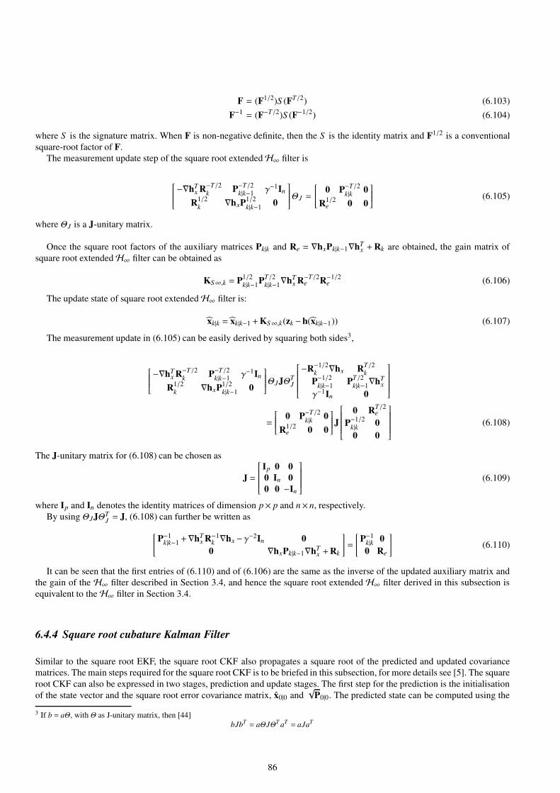
F = (F1/2)S (FT/2) (6.103)
F−1 = (F−T/2)S (F−1/2) (6.104)
where S is the signature matrix. When F is non-negative definite, then the S is the identity matrix and F1/2 is a conventional
square-root factor of F.
The measurement update step of the square root extendedH∞ filter is
−∇hT
x R−T/2
kP−T/2
k|k−1γ−1In
R1/2
k∇hxP
1/2
k|k−10
ΘJ =
0 P
−T/2
k|k 0
R1/2e 0 0
(6.105)
where ΘJ is a J-unitary matrix.
Once the square root factors of the auxiliary matrices Pk|k and Re = ∇hxPk|k−1∇hTx +Rk are obtained, the gain matrix of
square root extendedH∞ filter can be obtained as
KS∞,k = P1/2
k|k−1P
T/2
k|k−1∇hT
x R−T/2e R
−1/2e (6.106)
The update state of square root extendedH∞ filter is:
xk|k = xk|k−1 +KS∞,k(zk −h(xk|k−1)) (6.107)
The measurement update in (6.105) can be easily derived by squaring both sides3,
−∇hT
x R−T/2
kP−T/2
k|k−1γ−1In
R1/2
k∇hxP
1/2
k|k−10
ΘJJΘTJ
−R−1/2
k∇hx R
T/2
k
P−1/2
k|k−1P
T/2
k|k−1∇hT
x
γ−1In 0
=
0 P
−T/2
k|k 0
R1/2e 0 0
J
0 RT/2e
P−1/2
k|k 0
0 0
(6.108)
The J-unitary matrix for (6.108) can be chosen as
J =
Ip 0 0
0 In 0
0 0 −In
(6.109)
where Ip and In denotes the identity matrices of dimension p× p and n×n, respectively.
By using ΘJJΘTJ= J, (6.108) can further be written as
[P−1
k|k−1+∇hT
x R−1k∇hx −γ−2In 0
0 ∇hxPk|k−1∇hTx +Rk
]=
[P−1
k|k 0
0 Re
](6.110)
It can be seen that the first entries of (6.110) and of (6.106) are the same as the inverse of the updated auxiliary matrix and
the gain of the H∞ filter described in Section 3.4, and hence the square root extended H∞ filter derived in this subsection is
equivalent to theH∞ filter in Section 3.4.
6.4.4 Square root cubature Kalman Filter
Similar to the square root EKF, the square root CKF also propagates a square root of the predicted and updated covariance
matrices. The main steps required for the square root CKF is to be briefed in this subsection, for more details see [5]. The square
root CKF can also be expressed in two stages, prediction and update stages. The first step for the prediction is the initialisation
of the state vector and the square root error covariance matrix, x0|0 and√
P0|0. The predicted state can be computed using the
3 If b = aΘ, with Θ as J-unitary matrix, then [44]
bJbT = aΘJΘT aT = aJaT
86

below procedure. First, calculate the cubature points
χi,k−1|k−1 = P12
k−1|k−1ξi + xk−1|k−1, i = 1, . . . ,2n
where ξi is the i− th element of the following set
√n
1
0...
0
, . . . ,
0...
0
1
,
−1
0...
0
, . . . ,
0...
0
−1
.
The cubature points need to be propagated through the nonlinear process model as
χ∗i,k−1|k−1 = f(χi,k−1|k−1,uk−1), i = 1, . . . ,2n.
Finally, the predicted state can be obtained as
xk|k−1 =1
2n
2n∑
i=1
χ∗i,k−1|k−1
The square root factor of the predicted error covariance is:
√Pk|k−1 =
[qr
(X∗i,k|k−1
√Qk−1
)T]T
(6.111)
where
X∗i,k|k−1 =1√2n
[χ∗1,k|k−1 − xk|k−1 χ
∗2,k|k−1 − xk|k−1
. . . χ∗2n,k|k−1 − xk|k−1
]. (6.112)
Once the predicted state and square root covariance factor of the square root CKF is obtained, the next step is to find the updated
state and updated square root updated covariance. The predicted measurement, zi,k|k−1, is
zi,k|k−1 = h(χi,k|k−1,uk) (6.113)
χi,k|k−1 =√
Pk|k−1ξi + xk|k−1. (6.114)
The square root factors of innovation covariance and cross covariance matrices are:
√Pzz,k|k−1 =
[qr
(Zk|k−1
√Rk
)T]T
(6.115)
Pxz,k|k−1 = Xk|k−1ZTk|k−1 (6.116)
where,
Zk|k−1 =1√2n
[z1,k|k−1 − zk|k−1 z2,k|k−1 − zk|k−1 . . . z2n,k|k−1 − zk|k−1
](6.117)
Xk|k−1 =1√2n
[X1,k|k−1 − xk|k−1 X2,k|k−1 − xk|k−1 . . . X2n,k|k−1 − xk|k−1
]. (6.118)
The updated state and the updated square root factor of the error covariance matrix can then be calculated from:
xk|k = xk|k−1 +Kk(zk − zk|k−1) (6.119)
√Pk|k =
[qr
(Xk|k−1 −KkZk|k−1 Kk
√Rk
)T]T
, (6.120)
where,
Kk =[Pxz,k|k−1
/√PT
zz,k|k−1
] /√Pzz,k|k−1. (6.121)
87

6.4.5 Square root cubature information filter
In this subsection, another information filter using the square root approach for nonlinear systems is introduced. This algorithm
is derived from SREIF [88] and CKF discussed earlier in the book, and is called as the square root cubature information filter
(SRCIF). The square root factors of covariance matrices can be found using the QR4 decomposition and the leftdivide operator.
Furthermore, this approach can be extended to the multi-sensor data fusion, too.
The SRCIF is detailed in Algorithm 12. As in (6.128), the square root factor of the predicted error covariance matrix is evaluated.
Similarly, the square root factor of the measurement error covariance matrix, PT/2
zz,k|k−1, can be evaluated. The estimated state
vector and the square root factor of the error covariance matrix required for SRCIF prediction can be recovered by using (6.137),
(6.22) and (6.23). The derived SRCIF can then be extended to the case of multiple sensor. The prediction stage of the SRCIF in
the multi-sensor state estimation is similar to that of SRCIF with a single sensor.
By using (6.143), (6.138) and (6.102), the multi-sensor SRCIF measurement update step can be derived as
[YS ,k|k−1 Y1,M,k|k−1 Y2,M,k|k−1 . . . YD,M,k|k−1
yTS ,k|k−1
zT1,k
YR,1,k zT2,k
YR,2,k . . . zTD,k
YR,D,k
]Θ
=
[YS ,k|k 0
yTS ,k|k ⋆
]. (6.122)
Squaring both sides of the above equation yields:
[YS ,k|k−1 Y1,M,k|k−1 Y2,M,k|k−1 . . . YD,M,k|k−1
yTS ,k|k−1 zT
1,kYR,1,k zT
2,kYR,2,k . . . zT
D,kYR,D,k
]ΘΘT
YTS ,k|k−1
yS ,k|k−1
YT1,M,k|k−1
YTR,1,k
z1,k
YT2,M,k|k−1
YTR,2,k
z2,k
......
YTD,M,k|k−1
YTR,1,k
zD,k
=
[YS ,k|k 0
yTS ,k|k ⋆
][YT
S ,k|k yS ,k|k0 ⋆
](6.123)
∑D
j=1 Y j,M,k|k−1YTj,M,k|k−1
+YS ,k|k−1YTS ,k|k−1
∑Dj=1 Y j,M,k|k−1YT
R, j,kz j,k +YS ,k|k−1yS ,k|k−1∑D
j=1 zTj,k
YR, j,kYTj,M,k|k−1
+ yTS ,k|k−1YT
S ,k|k−1
∑Dj=1 z j,kYR, j,kYT
R, j,kz j,k + yT
S ,k|k−1YTS ,k|k−1
=
YS ,k|kYTS ,k|k YS ,k|kyS ,k|k
yTS ,k|kYT
S ,k|k ⋆
.(6.124)
4 QR is the orthogonal triangular decomposition and can be found in MATLAB using the command ‘qr’ .
88
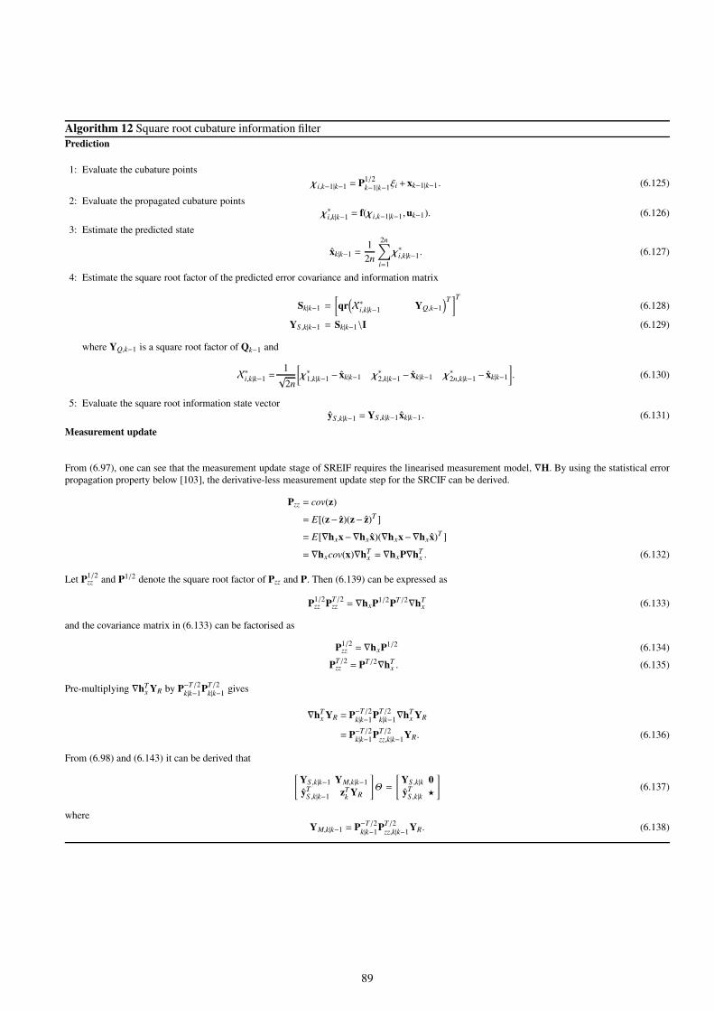
Algorithm 12 Square root cubature information filter
Prediction
1: Evaluate the cubature points
χi,k−1|k−1 = P1/2
k−1|k−1ξi +xk−1|k−1. (6.125)
2: Evaluate the propagated cubature points
χ∗i,k|k−1 = f(χi,k−1|k−1,uk−1). (6.126)
3: Estimate the predicted state
xk|k−1 =1
2n
2n∑
i=1
χ∗i,k|k−1. (6.127)
4: Estimate the square root factor of the predicted error covariance and information matrix
Sk|k−1 =
[qr
(X∗i,k|k−1 YQ,k−1
)T]T
(6.128)
YS ,k|k−1 = Sk|k−1\I (6.129)
where YQ,k−1 is a square root factor of Qk−1 and
X∗i,k|k−1 =1√2n
[χ∗1,k|k−1 − xk|k−1 χ
∗2,k|k−1 − xk|k−1 χ
∗2n,k|k−1 − xk|k−1
]. (6.130)
5: Evaluate the square root information state vector
yS ,k|k−1 =YS ,k|k−1xk|k−1. (6.131)
Measurement update
From (6.97), one can see that the measurement update stage of SREIF requires the linearised measurement model, ∇H. By using the statistical error
propagation property below [103], the derivative-less measurement update step for the SRCIF can be derived.
Pzz = cov(z)
= E[(z− z)(z− z)T ]
= E[∇hxx−∇hxx)(∇hxx−∇hxx)T ]
= ∇hxcov(x)∇hTx = ∇hxP∇hT
x . (6.132)
Let P1/2zz and P1/2 denote the square root factor of Pzz and P. Then (6.139) can be expressed as
P1/2zz P
T/2zz = ∇hxP1/2PT/2∇hT
x (6.133)
and the covariance matrix in (6.133) can be factorised as
P1/2zz = ∇hxP1/2 (6.134)
PT/2zz = PT/2∇hT
x . (6.135)
Pre-multiplying ∇hTx YR by P
−T/2
k|k−1P
T/2
k|k−1gives
∇hTx YR = P
−T/2
k|k−1P
T/2
k|k−1∇hT
x YR
= P−T/2
k|k−1P
T/2
zz,k|k−1YR. (6.136)
From (6.98) and (6.143) it can be derived that
[YS ,k|k−1 YM,k|k−1
yTS ,k|k−1
zTk
YR
]Θ =
[YS ,k|k 0
yTS ,k|k ⋆
](6.137)
where
YM,k|k−1 = P−T/2
k|k−1P
T/2
zz,k|k−1YR. (6.138)
89
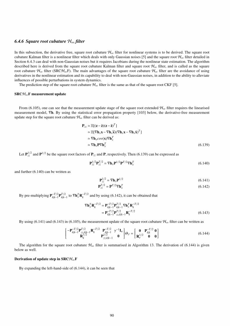
6.4.6 Square root cubatureH∞ filter
In this subsection, the derivative free, square root cubature H∞ filter for nonlinear systems is to be derived. The square root
cubature Kalman filter is a nonlinear filter which deals with only Gaussian noises [5] and the square rootH∞ filter detailed in
Section 6.4.3 can deal with non-Gaussian noises but it requires Jacobians during the nonlinear state estimation. The algorithm
described here is derived from the square root cubature Kalman filter and square root H∞ filter, and is called as the square
root cubature H∞ filter (SRCH∞F). The main advantages of the square root cubature H∞ filter are the avoidance of using
derivatives in the nonlinear estimation and its capability to deal with non-Gaussian noises, in addition to the ability to alleviate
influences of possible perturbations in system dynamics.
The prediction step of the square root cubatureH∞ filter is the same as that of the square root CKF [5].
SRCH∞F measurement update
From (6.105), one can see that the measurement update stage of the square root extended H∞ filter requires the linearised
measurement model, ∇h. By using the statistical error propagation property [103] below, the derivative-free measurement
update step for the square root cubatureH∞ filter can be derived as:
Pzz ≃ E[(z− z)(z− z)T ]
≃ E[∇hxx−∇hxx)(∇hxx−∇hxx)T ]
≃ ∇hxcov(x)∇hTx
≃ ∇hxP∇hTx (6.139)
Let P1/2zz and P1/2 be the square root factors of Pzz and P, respectively. Then (6.139) can be expressed as
P1/2zz P
T/2zz = ∇hxP1/2PT/2∇hT
x (6.140)
and further (6.140) can be written as
P1/2zz = ∇hxP1/2 (6.141)
PT/2zz = PT/2∇hT
x (6.142)
By pre-multiplying P−T/2
k|k−1P
T/2
k|k−1to ∇hT
x R−T/2
kand by using (6.142), it can be obtained that
∇hTx R−T/2
k= P
−T/2
k|k−1P
T/2
k|k−1∇hT
x R−T/2
k
= P−T/2
k|k−1P
T/2
zz,k|k−1R−T/2
k(6.143)
By using (6.141) and (6.143) in (6.105), the measurement update of the square root cubatureH∞ filter can be written as
−P−T/2
k|k−1P
T/2
zz,k|k−1R−T/2
kP−T/2
k|k−1γ−1In
R1/2
kP
1/2
zz,k|k−10
ΘJ =
0 P
−T/2
k|k 0
R1/2e 0 0
(6.144)
The algorithm for the square root cubature H∞ filter is summarised in Algorithm 13. The derivation of (6.144) is given
below as well.
Derivation of update step in SRCH∞F
By expanding the left-hand-side of (6.144), it can be seen that
90

−P−T/2
k|k−1P
T/2
zz,k|k−1R−T/2 P
−T/2
k|k−1γ−1In
R1/2 P1/2
zz,k|k−10
ΘJJΘTJ
−R−1/2P1/2
zz,k|k−1P−1/2
k|k−1RT/2
P−1/2
k|k−1P
T/2
zz,k|k−1
γ−1In 0
=
0 P
−T/2
k|k 0
R1/2e 0 0
J
0 RT/2e
P−1/2
k|k 0
0 0
(6.145)
By using ΘJJΘTJ= J and (6.109); (6.145) can be written as
[P−1
k|k−1+P−T/2
k|k−1P
T/2
zz,k|k−1R−1
kP
1/2
zz,k|k−1P−1/2
k|k−1−γ−2In 0
0 Pzz,k|k−1 +Rk
]=
[P−1
k|k 0
0 Re
](6.146)
By using the statistical approximations (6.69) and (6.142), the following can be derived:
Pxz,k|k−1 ≃ Pk|k−1∇hTx
= P1/2
k|k−1P
T/2
k|k−1∇hT
x
= P1/2
k|k−1(∇hxP
1/2
k|k−1)T
= P1/2
k|k−1P
T/2
zz,k|k−1(6.147)
By equating the corresponding terms of LHS and RHS of (6.146) and by using (6.147) in (6.146) it yields
P−1k|k = P−1
k|k−1 +P−1k|k−1Pxz,k|k−1R−1
k PTxz,k|k−1P−T
k|k−1 −γ−2In (6.148)
and
Re = Pzz,k|k−1 +Rk (6.149)
which is same as (6.74) in the cubatureH∞ filter.
91
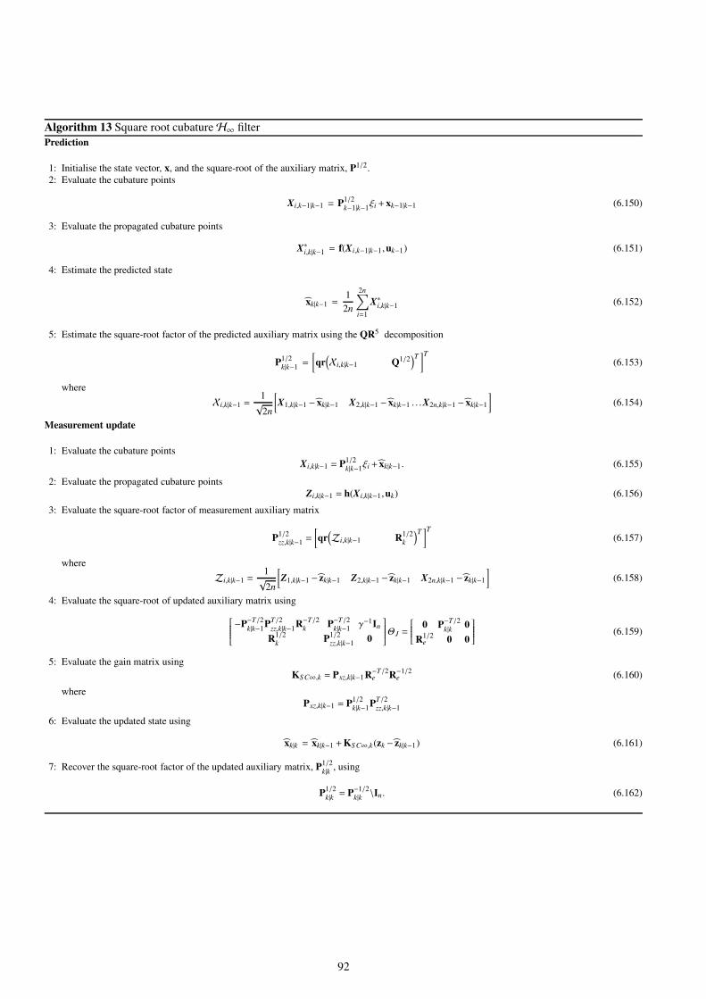
Algorithm 13 Square root cubatureH∞ filter
Prediction
1: Initialise the state vector, x, and the square-root of the auxiliary matrix, P1/2.
2: Evaluate the cubature points
Xi,k−1|k−1 = P1/2
k−1|k−1ξi +xk−1|k−1 (6.150)
3: Evaluate the propagated cubature points
X∗i,k|k−1 = f(Xi,k−1|k−1,uk−1) (6.151)
4: Estimate the predicted state
xk|k−1 =1
2n
2n∑
i=1
X∗i,k|k−1 (6.152)
5: Estimate the square-root factor of the predicted auxiliary matrix using the QR5 decomposition
P1/2
k|k−1=
[qr
(Xi,k|k−1 Q1/2
)T]T
(6.153)
where
Xi,k|k−1 =1√2n
[X1,k|k−1 − xk|k−1 X2,k|k−1 − xk|k−1 . . .X2n,k|k−1 − xk|k−1
](6.154)
Measurement update
1: Evaluate the cubature points
Xi,k|k−1 = P1/2
k|k−1ξi + xk|k−1. (6.155)
2: Evaluate the propagated cubature points
Zi,k|k−1 = h(Xi,k|k−1,uk) (6.156)
3: Evaluate the square-root factor of measurement auxiliary matrix
P1/2
zz,k|k−1=
[qr
(Zi,k|k−1 R
1/2
k
)T]T
(6.157)
where
Zi,k|k−1 =1√2n
[Z1,k|k−1 − zk|k−1 Z2,k|k−1 − zk|k−1 X2n,k|k−1 − zk|k−1
](6.158)
4: Evaluate the square-root of updated auxiliary matrix using
−P−T/2
k|k−1P
T/2
zz,k|k−1R−T/2k
P−T/2
k|k−1γ−1In
R1/2
kP
1/2
zz,k|k−10
ΘJ =
0 P
−T/2
k|k 0
R1/2e 0 0
(6.159)
5: Evaluate the gain matrix using
KS C∞,k = Pxz,k|k−1R−T/2e R
−1/2e (6.160)
where
Pxz,k|k−1 = P1/2
k|k−1P
T/2
zz,k|k−1
6: Evaluate the updated state using
xk|k = xk|k−1 +KS C∞,k(zk − zk|k−1) (6.161)
7: Recover the square-root factor of the updated auxiliary matrix, P1/2
k|k , using
P1/2
k|k = P−1/2
k|k \In. (6.162)
92

6.4.7 Square root cubatureH∞ information filter
In this subsection, a numerically stable square root version of the cubatureH∞ information filter (SRCH∞IF) is to be developed.
Square root filters arise when the covariance or information matrices are replaced by their square root factors; these square root
factors are then propagated at various stages. Square root factors for the information matrix and other matrices are defined such
that
I = IsITs (6.163)
Pxz = Pxz,sPTxz,s (6.164)
R−1 = RsiRTsi (6.165)
Q = QsQTs (6.166)
where Is = P−T2 , Pxz,s = P
12xz,s, Rsi = R
−T2 , and Qs =Q
12 . Note that these square root factors are not unique and can be calculated
using different numerical techniques such as the QR decomposition, etc..
The square root cubature H∞ information filter (SRCH∞IF) also comprises prediction and update stages. The prediction
stage in SRCH∞IF is the same as that of the square root CKF, see Section 6.4.4 earlier in this chapter, also in [5], but the
information vector and the square root of the information matrix are propagated rather than the state and covariance matrix in
the updating procedure.
The prediction stage of SRCH∞IF has straight forward equations, please see the prediction stage of Algorithm 13 for more
details. However, the update stage is not that straight forward. The update stage for the square root cubature H∞ information
filter using the J-orthogonal transformation is given in the theorem below.
Theorem 6.1. The updated information vector and information matrix for the SRCH∞IF can be obtained from
[Is,k|k−1Pzz,s,k|k−1Rsi,k Is,k|k−1 γ−1In
zTa,k
Rsi,k sTs,k|k−1
0
]ΘJ =
[Is,k|k 0 0
sTs,k|k 0 ⋆
], (6.167)
where ⋆ represent the terms which are irrelevant for the SRCH∞IF, za,k = νk +PTzz,s,k|k−1
ITs,k|k−1
xk|k−1 and ΘJ is a J-unitary
matrix which satisfies
ΘJΘTJ = J and J =
In 0 0
0 In 0
0 0 −In
.
Proof. Squaring the left hand side (LHS) of (6.167) yields
[Is,k|k−1Pzz,s,k|k−1Rsi,k Is,k|k−1 γ−1In
zTa,k
Rsi,k sTs,k|k−1
0
]ΘJΘ
TJ
RTsi,k
PTzz,s,k|k−1
ITs,k|k−1
RTsi,k
za,k
ITs,k|k−1
ss,k|k−1
γ−1In 0
, (6.168)
Further, (6.168) can be written as
[Is,k|k−1Pzz,s,k|k−1Rsi,k Is,k|k−1 γ−1In
zTa,k
Rsi,k sTs,k|k−1
0
]In 0 0
0 In 0
0 0 −In
RTsi,k
PTzz,s,k|k−1
ITs,k|k−1
RTsi,k
za,k
ITs,k|k−1
ss,k|k−1
γ−1In 0
,
=
[ (Is,k|k−1Pzz,s,k|k−1R−1k
PTzz,s,k|k−1
ITs,k|k−1
+Ik|k−1 −γ−2In) (Is,k|k−1Pzz,s,k|k−1R−1
kza,k +Is,k|k−1ss,k|k−1
)
⋆ ⋆
](6.169)
The covariance matrix in (6.82) can be factorised as
Pzz,k|k−1 = ∇hPk|k−1∇hT
= ∇hP12
k|k−1P
T2
k|k−1∇hT
= (∇hPs,k|k−1)(∇hPs,k|k−1)T
= Pzz,s,k|k−1PTzz,s,k|k−1. (6.170)
The Pxz,k|k−1 in (6.83) can be represented in terms of Pzz,s,k|k−1 and Ps,k|k−1 as
93

Pxz,k|k−1 = Pk|k−1∇hT
= P12
k|k−1(∇hP
12
k|k−1)T
= Ps,k|k−1PTzz,s,k|k−1 (6.171)
Pre-multiplying the information matrix on both sides of the aforementioned equation yields
Ik|k−1Pxz,k|k−1 = Ik|k−1Ps,k|k−1PTzz,s,k|k−1
= Is,k|k−1ITs,k|k−1Ps,k|k−1PT
zz,s,k|k−1
= Is,k|k−1PTzz,s,k|k−1 (6.172)
Substituting (6.172) in (6.169) yields
[ (Ik|k−1Pxz,k|k−1R−1k
PTxz,k|k−1
ITk|k−1+Ik|k−1 −γ−2
In) (Ik|k−1Pxz,k|k−1R−1
kza,k +Is,k|k−1ss,k|k−1
)
⋆ ⋆
]
=
[ (Ik|k−1 +Ik|k−1Pxz,k|k−1R−1k
PTxz,k|k−1
ITk|k−1−γ−2
In) (sk|k−1 +Ik|k−1Pxz,k|k−1R−1
kza,k
)
⋆ ⋆
]. (6.173)
Now by squaring the right hand side (RHS) of the update stage in (6.167), the following can be derived
[Is,k|k 0 0
sTs,k|k 0 ⋆
]
ITs,k|k ss,k|k0 0
0 ⋆
=
[Ik|kITs,k|k Is,k|kss,k|k
⋆ ⋆
]
=
[Is,k|k sk|k⋆ ⋆
]. (6.174)
By equating the corresponding elements of (6.173) and (6.174), which corresponds to the LHS and RHS of (6.167), one gets
sk|k = sk|k−1 + ik (6.175)
Ik|k = Ik|k−1 + Ik. (6.176)
where
ik = Ik|k−1Pxz,k|k−1R−1k [νk +PT
xz,k|k−1ITk|k−1xk|k−1] (6.177)
Ik = Ik|k−1Pxz,k|k−1R−1k PT
xz,k|k−1ITk|k−1 −γ−2
In. (6.178)
Note that the information vector and the information matrix given in (6.175) and (6.176), and the corresponding information
contributions in (6.177) and (6.178) for the SRCH∞IF are the same as those of the CH∞IF in (6.80), (6.81), (6.85) and (6.86).
This proves that the update stage of the SRCH∞IF given in Theorem 6.1 is an equivalent of the CH∞IF in Section 6.3.4.
The prediction stage of multi-sensor SRCH∞IF will be the same as that of the single sensor SRCH∞IF, since the multiple
sensors only affect the update stage. The updated information vector and information matrix of the multi-sensor SRCH∞IF can
be obtained from
[Is,k|k−1Pzz,1,s,k|k−1Rsi,1,k Is,k|k−1Pzz,2,s,k|k−1Rsi,2,k . . . Is,k|k−1Pzz,D,s,k|k−1Rsi,D,k Is,k|k−1 γ
−1I
za,1,k za,2,k . . . za,D,k sk|k−1 0
]ΘJ =
[Is,k|k 0 0
ss,k|k 0 ⋆
](6.179)
The update stage for multi-sensor SRCH∞IF in (6.179) can easily be proved along the similar lines of the proof of Theorem
6.1. The square root cubatureH∞ information filters for the single sensor and multi-sensors are summarised in Algorithm 14.
Apart from its applicability for the multi-sensor state estimations in the presence of Gaussian or non-Gaussian noises,
SRCH∞IF can also handle the case of ill-conditioned covariance matrices and it possesses double order precision in the com-
putation. As such, the square root cubature H∞ information filters are suitable for efficient, real-time implementations. They
can also easily estimate the states with near-perfect measurements and/or in cases of systems with uncertainties up to a certain
degree.
94

Algorithm 14 Square root cubatureH∞ information filter
Initialise the information vector and square-root information matrix, Is,0|0 and ss,0|0 for k = 1.
Prediction
1: Evaluate χi,k−1|k−1, χ∗i,k|k−1
and xk|k−1 as
χi,k−1|k−1 =(Is,k−1|k−1\In
)ξi + (Is,k−1|k−1\ss,k−1|k−1),
χ∗i,k|k−1 = f(χi,k−1|k−1,uk−1)
xk|k−1 =1
2n
2n∑
i=1
χ∗i,k|k−1
where ‘\’ is the left-divide operator, In is the nth order identity matrix, and ξi is the i-th element of the following set
√n
1
0
.
.
.
0
, . . . ,
0
.
.
.
0
1
,
−1
0
.
.
.
0
, . . . ,
0
.
.
.
0
−1
(6.180)
2: Evaluate the information matrix
Is,k|k−1 =
[qr
(X∗i,k|k−1 Qs,k−1
)T]T
∖In
ss,k|k−1 = Is,k|k−1xk|k−1
where
X∗i,k|k−1 =1√2n
[χ∗1,k|k−1 − xk|k−1 χ
∗2,k|k−1 − xk|k−1 . . . χ
∗2n,k|k−1 − xk|k−1
].
Measurement update
1: Evaluate χi,k|k−1, Zi,k|k−1 and zk|k−1 as
χi,k|k−1 = Is,k|k−1\Inξi +xk|k−1
Zi,k|k−1 = h(χi,k|k−1,uk)
zk|k−1 =1
2n
2n∑
i=1
Zi,k|k−1.
2: Evaluate
Pzz,s,k|k−1 =[qr
(Zi,k|k−1 Rsi,k
)T]T
∖
where
Zi,k|k−1 =1√2n
[Z1,k|k−1 − zk|k−1 Z2,k|k−1 − zk|k−1 . . . Z2n,k|k−1 − zk|k−1
].
3: For a single sensor, the square root information matrix and the corresponding information vector can be obtained from
[Is,k|k−1Pzz,s,k|k−1Rsi,k Is,k|k−1 γ
−1In
zTa,k
Rsi,k sTs,k|k−1
0
]ΘJ =
[Is,k|k 0 0
sTs,k|k 0 ⋆
],
where γ is an attenuation parameter, ΘJ is a J-unitary matrix, za,k = νk +PTzz,s,k|k−1
ITs,k|k−1
xk|k−1, and ⋆ represent the terms which are irrelevant for
the SR-CH∞IF.
Measurement update for multi-sensor state estimation
1: For the case of multiple sensors, the square root information matrix and the corresponding information vector can be obtained from
[Is,k|k−1Pzz,1,s,k|k−1Rsi,1,k Is,k|k−1Pzz,2,s,k|k−1Rsi,2,k . . . Is,k|k−1Pzz,D,s,k|k−1Rsi,D,k Is,k|k−1 γ
−1In
za,1,k za,2,k . . . za,D,k sk|k−1 0
]ΘJ =
[Is,k|k 0 0
ss,k|k 0 ⋆
]
95
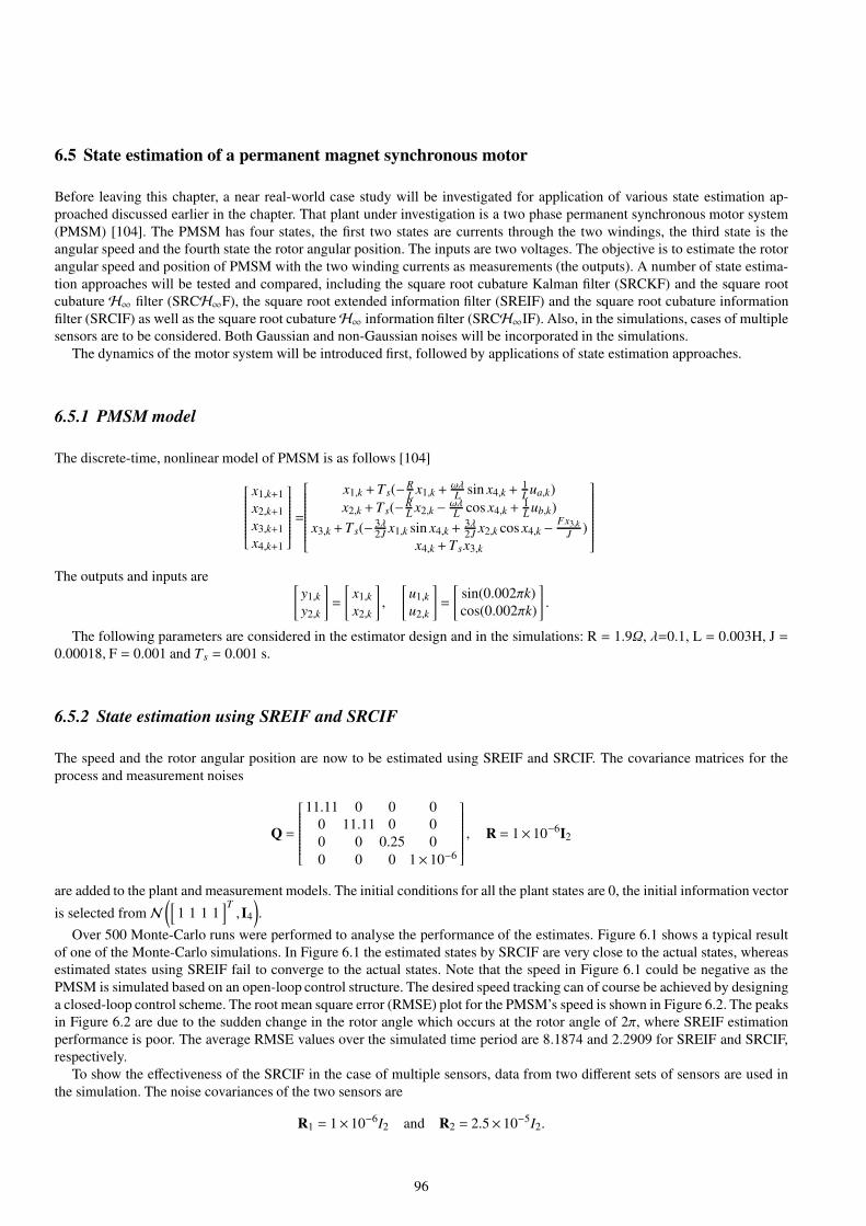
6.5 State estimation of a permanent magnet synchronous motor
Before leaving this chapter, a near real-world case study will be investigated for application of various state estimation ap-
proached discussed earlier in the chapter. That plant under investigation is a two phase permanent synchronous motor system
(PMSM) [104]. The PMSM has four states, the first two states are currents through the two windings, the third state is the
angular speed and the fourth state the rotor angular position. The inputs are two voltages. The objective is to estimate the rotor
angular speed and position of PMSM with the two winding currents as measurements (the outputs). A number of state estima-
tion approaches will be tested and compared, including the square root cubature Kalman filter (SRCKF) and the square root
cubature H∞ filter (SRCH∞F), the square root extended information filter (SREIF) and the square root cubature information
filter (SRCIF) as well as the square root cubatureH∞ information filter (SRCH∞IF). Also, in the simulations, cases of multiple
sensors are to be considered. Both Gaussian and non-Gaussian noises will be incorporated in the simulations.
The dynamics of the motor system will be introduced first, followed by applications of state estimation approaches.
6.5.1 PMSM model
The discrete-time, nonlinear model of PMSM is as follows [104]
x1,k+1
x2,k+1
x3,k+1
x4,k+1
=
x1,k +Ts(−RL
x1,k +ωλL
sin x4,k +1L
ua,k)
x2,k +Ts(−RL
x2,k − ωλL
cos x4,k +1L
ub,k)
x3,k +Ts(− 3λ2J
x1,k sin x4,k +3λ2J
x2,k cos x4,k − Fx3,k
J)
x4,k +Tsx3,k
The outputs and inputs are [y1,k
y2,k
]=
[x1,k
x2,k
],
[u1,k
u2,k
]=
[sin(0.002πk)
cos(0.002πk)
].
The following parameters are considered in the estimator design and in the simulations: R = 1.9Ω, λ=0.1, L = 0.003H, J =
0.00018, F = 0.001 and Ts = 0.001 s.
6.5.2 State estimation using SREIF and SRCIF
The speed and the rotor angular position are now to be estimated using SREIF and SRCIF. The covariance matrices for the
process and measurement noises
Q =
11.11 0 0 0
0 11.11 0 0
0 0 0.25 0
0 0 0 1×10⁻⁶
, R = 1×10⁻⁶I2
are added to the plant and measurement models. The initial conditions for all the plant states are 0, the initial information vector
is selected fromN([
1 1 1 1]T,I4
).
Over 500 Monte-Carlo runs were performed to analyse the performance of the estimates. Figure 6.1 shows a typical result
of one of the Monte-Carlo simulations. In Figure 6.1 the estimated states by SRCIF are very close to the actual states, whereas
estimated states using SREIF fail to converge to the actual states. Note that the speed in Figure 6.1 could be negative as the
PMSM is simulated based on an open-loop control structure. The desired speed tracking can of course be achieved by designing
a closed-loop control scheme. The root mean square error (RMSE) plot for the PMSM’s speed is shown in Figure 6.2. The peaks
in Figure 6.2 are due to the sudden change in the rotor angle which occurs at the rotor angle of 2π, where SREIF estimation
performance is poor. The average RMSE values over the simulated time period are 8.1874 and 2.2909 for SREIF and SRCIF,
respectively.
To show the effectiveness of the SRCIF in the case of multiple sensors, data from two different sets of sensors are used in
the simulation. The noise covariances of the two sensors are
R1 = 1×10⁻⁶I2 and R2 = 2.5×10⁻⁵I2.
96
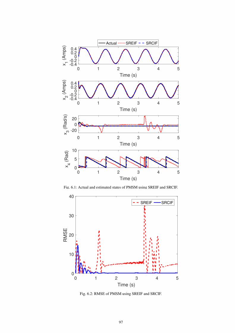
0 1 2 3 4 5
Time (s)
-0.4-0.2
00.20.4
x1 (
Am
ps)
Actual SREIF SRCIF
0 1 2 3 4 5
Time (s)
-0.4-0.2
00.20.4
x2 (
Am
ps)
0 1 2 3 4 5
Time (s)
-20
0
20
x3 (
Ra
d/s
)
0 1 2 3 4 5
Time (s)
0
5
10
x4 (
Ra
d)
Fig. 6.1: Actual and estimated states of PMSM using SREIF and SRCIF.
0 1 2 3 4 5
Time (s)
0
10
20
30
40
RM
SE
SREIF SRCIF
Fig. 6.2: RMSE of PMSM using SREIF and SRCIF.
97
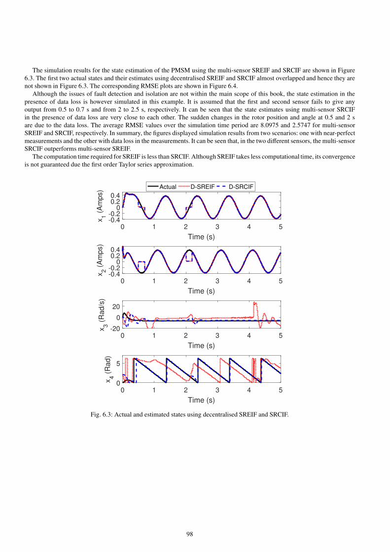
The simulation results for the state estimation of the PMSM using the multi-sensor SREIF and SRCIF are shown in Figure
6.3. The first two actual states and their estimates using decentralised SREIF and SRCIF almost overlapped and hence they are
not shown in Figure 6.3. The corresponding RMSE plots are shown in Figure 6.4.
Although the issues of fault detection and isolation are not within the main scope of this book, the state estimation in the
presence of data loss is however simulated in this example. It is assumed that the first and second sensor fails to give any
output from 0.5 to 0.7 s and from 2 to 2.5 s, respectively. It can be seen that the state estimates using multi-sensor SRCIF
in the presence of data loss are very close to each other. The sudden changes in the rotor position and angle at 0.5 and 2 s
are due to the data loss. The average RMSE values over the simulation time period are 8.0975 and 2.5747 for multi-sensor
SREIF and SRCIF, respectively. In summary, the figures displayed simulation results from two scenarios: one with near-perfect
measurements and the other with data loss in the measurements. It can be seen that, in the two different sensors, the multi-sensor
SRCIF outperforms multi-sensor SREIF.
The computation time required for SREIF is less than SRCIF. Although SREIF takes less computational time, its convergence
is not guaranteed due the first order Taylor series approximation.
0 1 2 3 4 5
Time (s)
-0.4-0.2
00.20.4
x1 (
Am
ps) Actual D-SREIF D-SRCIF
0 1 2 3 4 5
Time (s)
-0.4-0.2
00.20.4
x2 (
Am
ps)
0 1 2 3 4 5
Time (s)
-20
0
20
x3 (
Ra
d/s
)
0 1 2 3 4 5
Time (s)
0
5
x4 (
Ra
d)
Fig. 6.3: Actual and estimated states using decentralised SREIF and SRCIF.
98
0 1 2 3 4 5
Time (s)
0
5
10
15
20
25
30
35
RM
SE
D-SREIF D-SRCIF
Fig. 6.4: RMSE of PMSM using decentralised SREIF and SRCIF.
6.5.3 State estimation using SRCKF and SRCH∞F
In this subsection, the state estimation algorithms of the square root cubature Kalman filter (SRCKF) and the square root
cubature H∞ filter (SRCH∞F) will be applied to estimate the first two states of the permanent magnet synchronous mo-
tor. The initial conditions for all the plant states are chosen as 0.1 and the initial estimated state vector is selected from
U
([0.1 0.1 0.1 0.1
]T,0.1× I4
).
6.5.3.1 State estimation in the presence of non-Gaussian noise
In this case the process and measurement noises are assumed to be non-Gaussian uniform distributed. For the process noise, the
standard deviations of the four states are 0.01, 0.01, 0.5 and 0.0001, and the standard deviations for the measurement noise are
0.05 and 0.05. The actual and estimated states, and the RMSEs using the square root CKF and square root cubatureH∞ filter are
shown in Figures 6.5 and 6.6, respectively. The RMSE for the square root CKF is higher than the square root cubatureH∞ filter.
The maximum RMSEs for the square root CKF and the square root cubature H∞ filter are 0.7113 and 0.3679, respectively.
Hence, for the PMSM also the square-root cubatureH∞ filter would appear to be well suited in the presence of non-Gaussian
noises.
6.5.3.2 State estimation with near-perfect measurements
In this scenario, the simulations above are repeated with near-perfect measurements. Two groups of results are demonstrated:
a) with non-Gaussian process noise; and, b) with Gaussian process noise. For the Gaussian case, the standard deviations of
the four states for process noise are the same as that of the non-Gaussian case as given earlier. The standard deviations of the
measurement noise are 1×10⁻¹⁵ and 1×10⁻¹⁵ for both Gaussian and non-Gaussian simulations. The corresponding results are
shown in the Figure 6.7. Similar to CSTR, the RMSEs using square root cubatureH∞ filters in the presence of Gaussian and
non-Gaussian are also within an acceptable range.
99

0 1 2 3 4 5
Time (s)
-0.4-0.2
00.20.4
x1 (
Am
ps)
Actual SRCKF SRCHF
0 1 2 3 4 5
Time (s)
-0.4-0.2
00.20.4
x2 (
Am
ps)
0 1 2 3 4 5
Time (s)
-20
0
20
x3 (
Ra
d/s
)
0 1 2 3 4 5
Time (s)
0
5
x4 (
Ra
d)
Fig. 6.5: Actual and estimated states of PMSM for non-Gaussian noise using SRCKF and SRCH∞F.
0 1 2 3 4 5
Time (s)
0
0.5
1
1.5
2
2.5
3
RM
SE
SRCKF SRCHF
Fig. 6.6: RMSEs of the PMSM using SRCKF and SRCH∞F.
100

0 1 2 3 4 5
Time (s)
0
0.2
0.4
0.6
RM
SE
of x
3 (
rad/s
) Gaussian Noise
0 1 2 3 4 5
Time (s)
0
0.05
0.1
0.15
0.2
RM
SE
of x
3 (
rad/s
) Non-Gaussian Noise
Fig. 6.7: RMSEs of x3 with near-perfect measurements for the PMSM using SRCKF and SRCH∞F.
101

6.5.4 State estimation with multi-sensors using SREIF, SRCIF and SRCH∞IF
In this part, the states of PMSM are to be estimated by using multiple sensors. The approach applied is mainly the square
root cubature H∞ information filter (SRCH∞IF), though other filters will be tested in simulations for comparison purpose.
Two scenarios are considered: a) state estimation in the presence of Gaussian noise; and, b) state estimation in the presence of
non-Gaussian noise.
6.5.4.1 Multi-sensor state estimation in the presence of low Gaussian noise
It is first assumed that the process and measurement noises are Gaussian. For all the simulation results given in this part, the ini-
tial conditions for the actual PMSM states and the information vector are randomly selected fromN([0.1 0.1 0.1 0.1]T ,0.1×I4).
SRCH∞IF. For multi-sensor state estimation, two sets of current sensors are used to estimate the states. The process and
measurement noise covariance matrices for are chosen as
Q =
6.25 0 0 0
0 6.25 0 0
0 0 0.1 0
0 0 0 1×10⁻⁶
, R1 =
[2.5×10⁻⁶ 0
0 2.5×10⁻⁶
]R2 =
[5×10⁻⁶ 0
0 5×10⁻⁶
]
Simulation results of state estimation in the presence of low-Gaussian noise using the multi-sensor SREH∞IF and SRCH∞IF
are shown in Figure 6.8. The actual states and their estimates using the SREH∞IF and SRCH∞IF are shown in Figure 6.8. The
estimates using the SREH∞IF are more erroneous than the SRCH∞IF. The root means square errors (RMSEs) for the speed
using SREH∞IF and SRCH∞IF are shown in Figure 6.9, where the SREH∞IF RMSE is larger than that of SRCH∞IF. The
maximum RMSE error is 58.6 for the SREH∞IF and 4.7 for the SRCH∞IF, and the average RMSE error is 12.89 for the
SREH∞IF and 1.21 for the SRCH∞IF.
6.5.4.2 Multi-sensor state estimation in the presence of high Gaussian noise
The simulations are now performed with high-Gaussian noise. It is assumed that the sensors and plant model used here are
more prone to noise such that their noise covariance matrices are assumed to be 12 times those given in last simulation with
low-Gaussian noise. The process and measurement noise covariance matrices for high-Gaussian noise are chosen as:
Q =
75 0 0 0
0 75 0 0
0 0 1.2 0
0 0 0 1.2×10⁻⁵
, R1 =
[3×10⁻⁵ 0
0 3×10⁻⁵
], R2 =
[6×10⁻⁵ 0
0 6×10⁻⁵
].
Simulation results of a typical simulation run are shown in Figure 6.10. The actual states and their estimates using the
SREH∞IF and SRCH∞IF are shown in Figure 6.10. Due to the noisy current sensors, the first two states (the currents of
PMSM) in Figure 6.10 are noisy. The root means square errors (RMSEs) for the speed using SREH∞IF and SRCH∞IF are
shown in Figure 6.11, where the SREH∞IF RMSE is larger than that of SRCH∞IF. The maximum RMSE error is 58.95 for the
SREH∞IF and 23.25 for SRCH∞IF, and the average RMSE error is 13.59 for SREH∞IF and 4.09 for SRCH∞IF.
6.5.4.3 Multi-sensor state estimation in the presence of low non-Gaussian noises
In some of the control engineering applications, the process and/or measurement noises can be approximated by a Rayleigh
probability distribution function [94]. In computer simulations, Rayleigh noise can be generated using the Matlab command
‘raylrnd’To demonstrate the efficacy of the state estimators in the presence of non-Gaussian noise, simulations are performed
for low and high intensity Rayleigh noises.
First we consider the case of low non-Gaussian noise. The process and measurement covariance matrices are the same as of
low Gaussian noise discussed earlier, however, the plant and measurements are corrupted by Rayleigh noise. Results of a typical
simulation run using the Rayleigh noise are shown in Figure 6.12. The actual states and their estimates using the SREH∞IF and
102
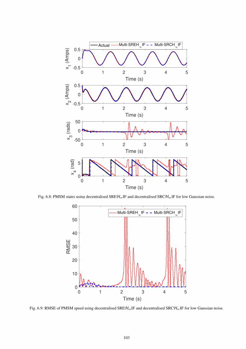
0 1 2 3 4 5
Time (s)
-0.5
0
0.5
x1 (
Am
ps)
Actual Multi-SREH∞
IF Multi-SRCH∞
IF
0 1 2 3 4 5
Time (s)
-0.5
0
0.5
x2 (
Am
ps)
0 1 2 3 4 5
Time (s)
-50
0
50
x3 (
rad
s)
0 1 2 3 4 5
Time (s)
0
5
x4 (
rad
)
Fig. 6.8: PMSM states using decentralised SREH∞IF and decentralised SRCH∞IF for low Gaussian noise.
0 1 2 3 4 5
Time (s)
0
10
20
30
40
50
60
RM
SE
Multi-SREH∞
IF Multi-SRCH∞
IF
Fig. 6.9: RMSE of PMSM speed using decentralised SREH∞IF and decentralised SRCH∞IF for low Gaussian noise.
103
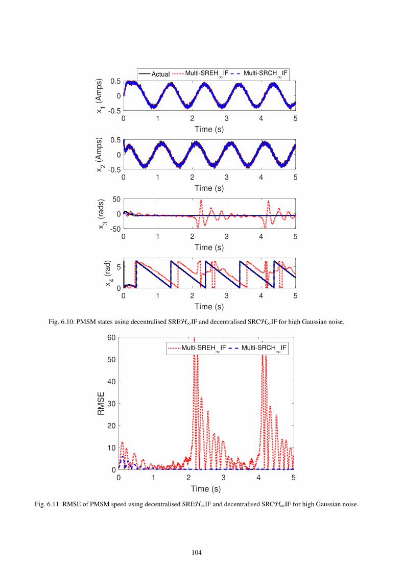
0 1 2 3 4 5
Time (s)
-0.5
0
0.5
x1 (
Am
ps)
Actual Multi-SREH∞
IF Multi-SRCH∞
IF
0 1 2 3 4 5
Time (s)
-0.5
0
0.5
x2 (
Am
ps)
0 1 2 3 4 5
Time (s)
-50
0
50
x3 (
rad
s)
0 1 2 3 4 5
Time (s)
0
5
x4 (
rad
)
Fig. 6.10: PMSM states using decentralised SREH∞IF and decentralised SRCH∞IF for high Gaussian noise.
0 1 2 3 4 5
Time (s)
0
10
20
30
40
50
60
RM
SE
Multi-SREH∞
IF Multi-SRCH∞
IF
Fig. 6.11: RMSE of PMSM speed using decentralised SREH∞IF and decentralised SRCH∞IF for high Gaussian noise.
104

0 1 2 3 4 5
Time (s)
-0.5
0
0.5
x1 (
Am
ps)
Actual Multi-SREH∞
IF Multi-SRCH∞
IF
0 1 2 3 4 5
Time (s)
-0.5
0
0.5
x2 (
Am
ps)
0 1 2 3 4 5
Time (s)
-50
0
50
x3 (
rad
s)
0 1 2 3 4 5
Time (s)
0
5
x4 (
rad
)
Fig. 6.12: PMSM states using decentralised SREH∞IF and decentralised SRCH∞IF for low non-Gaussian noise.
0 1 2 3 4 5
Time (s)
0
10
20
30
40
50
60
RM
SE
Multi-SREH∞
IF Multi-SRCH∞
IF
Fig. 6.13: RMSE of PMSM speed using decentralised SREH∞IF and decentralised SRCH∞IF for low non-Gaussian noise.
105

0 1 2 3 4 5
Time (s)
-0.5
0
0.5
x1 (
Am
ps)
Actual Multi-SREH∞
IF Multi-SRCH∞
IF
0 1 2 3 4 5
Time (s)
-0.5
0
0.5
x2 (
Am
ps)
0 1 2 3 4 5
Time (s)
-50
0
50
x3 (
rad
s)
0 1 2 3 4 5
Time (s)
0
5
x4 (
rad
)
Fig. 6.14: PMSM states using decentralised SREH∞IF and decentralised SRCH∞IF for high non-Gaussian noise.
0 1 2 3 4 5
Time (s)
0
10
20
30
40
50
RM
SE
Multi-SREH∞
IF Multi-SRCH∞
IF
Fig. 6.15: RMSE of PMSM speed using decentralised SREH∞IF and decentralised SRCH∞IF for high non-Gaussian noise.
106

0 1 2 3 4 50
0.5
1
1.5
2
2.5
3
3.5
Time (s)
RM
SE
Gaussian Noise Non−Gaussian Noise
0.24 0.26 0.28 0.3
1.391.4
1.411.421.43
0.12 0.14 0.16 0.18 0.2
3.15
3.2
Fig. 6.16: PMSM simulation results in the presence of near-perfect Gaussian and non-Gaussian noise in multi-sensor SRCH∞IF.
SRCH∞IF are shown in Figure 6.12. In this case also the first two states and their estimates using SREH∞IF and SRCH∞IF
almost overlap and estimation errors of speed and rotor position using the SREH∞IF are larger. The RMSEs for the speed
using SREH∞IF and SRCH∞IF are shown in Figure 6.13. The maximum RMSE error is 39.74 for the SREH∞IF and 8.24 for
SRCH∞IF, and the average RMSE error is 12.89 for the SREH∞IF and 1.64 for SRCH∞IF.
6.5.4.4 Multi-sensor state estimation in the presence of high non-Gaussian noise
We now consider the case of high, non-Gaussian noise. The process and measurement covariance matrices are the same as
of high Gaussian noise, but the plant and measurements are corrupted by Rayleigh noise. Results of a typical simulation run
using the high intensity Rayleigh noise are shown in Figure 6.14. The actual states and their estimates using the SREH∞IF and
SRCH∞IF are shown in Figure 6.14. The first two states are seen to be noisy due to the high intensity Rayleigh noise added
to them. In this case also the first two states and their estimates using SREH∞IF and SRCH∞IF almost overlap and estimation
errors of speed and rotor position using the SREH∞IF are larger. The RMSEs for the speed using SREH∞IF and SRCH∞IF
are shown in Figure 6.15. The maximum RMSE error is 48.37 for the SREH∞IF and 32 for SRCH∞IF, and the average RMSE
error is 12.82 for the SREH∞IF and 5.52 for SRCH∞IF.
6.5.4.5 Multi-sensor state estimation in the presence of near-perfect measurements
This part presents the simulation results with near-perfect plant and measurement models in the presence of Gaussian and
non-Gaussian noise. It is assumed that the sensors provide near-perfect measurements and the process models are also almost
perfect. The process and measurement noise covariance matrices are chosen as:
Q =
1×10⁻²⁰ 0 0 0
0 1×10⁻²⁰ 0 0
0 0 1×10⁻²⁰ 0
0 0 0 1×10⁻²⁰
,R1 =
[1×10⁻²⁰ 0
0 1×10⁻²⁰
],R2 =
[1×10⁻²⁰ 0
0 1×10⁻²⁰
].
The square root filters have inherent tendency to effectively estimate the states in the presence of near-perfect measurements,
for more details please see [109], [40], [104], [21]. The estimated and actual states with near-perfect measurements are very
close for both the Gaussian and Rayleigh noises, and hence the plots of states and their estimates are not shown. The root means
square errors (RMSEs) for the speed in the presence of Gaussian and non-Gaussian noise using multi-sensor SRCH∞IF are
shown in Figure 6.16. The RMSE errors for both cases are very low. The maximum RMSE error is 3.18 for the Gaussian noise
107

and 3.19 for the Rayleigh noise, and the average RMSE error is 0.5816 for the Gaussian noise and 0.5869 for the non-Gaussian
noise respectively.
Since the square root extended H∞ information filter is a Jacobian based approach, it is sometimes difficult to implement
on various applications for example when the Jacobians are ill-conditioned or for piecewise nonlinear systems. However, the
square root cubatureH∞ information filter is a Jacobian free approach and hence one can avoid the difficulties due to Jacobians.
The simulation results in this numerical example show the efficacy of SRCH∞IF. It can be observed that this type of filter has
a tendency to handle low and high Gaussian noises and non-Gaussian noises as well. Further, the square root cubature H∞information filter can be very useful in applications where the sensor-measurements are near-perfect. This shows that the
square root cubature hin f information filter has certain robustness, the property will be touched upon in the next chapter.
The simulations have been performed using 64 bit Matlab on a computer with the processor speed on 3.4 GHz. The average
computation time, for the simulations included in this example, are 3.1 s and 3.6 s for SREH∞IF and SRCH∞IF, respectively.
However, it can be seen that in all the simulations the quality of the state estimate using SRCH∞IF is far better than SREH∞IF.
6.6 State estimation of a continuous stirred tank reactor (CSTR)
In this section, a continuous stirred tank reactor (CSTR) system is to be considered. The state of CSTR will be estimated in
the presence of Gaussian and non-Gaussian noises, in order to evaluate the performance of the square root cubatureH∞ filter
(SRCH∞F) in comparison with the performance of the square root cubature Kalman filter (SRCKF).
6.6.1 The model
The process model for an irreversible, first-order chemical reaction, A→ B which occurs in the continuous stirred tank reactor
(CSTR) is as follows [110], [69]
CA =q
V(CA f −CA)− k0 exp
(−E
RT
)CA (6.181)
T =q
V(T f −T )+
−∇H
ρCp
k0 exp
(−E
RT
)CA+
UA
VρCp
(Tc−T ) (6.182)
The state variables are the concentration, CA, and the temperature of the reactor, T ; the measured output, h, depends on the
temperature T .
The following parameters are considered in the simulations [69]:
q = 100L/min, ER= 8750K, CA f = 1mol/L, K0 = 7.5× 10¹⁰min−1, T f = 350K, UA = 5000J/minK, V = 100L, Tc = 300K,
ρ = 1000g/L, CA = 0.5mol/L, Cp = 0.239J/gK, T = 350K and (∇H) = 5000J/mol.
The process and measurement noises, wk and vk, are added to the process and measurement models, respectively. The control
variable, the coolant temperature Tc, is computed using the input-output feedback linearisation [69]
Tc =ζ − L f h(x)
Lgh(x)(6.183)
The Lie derivatives L f and Lg, and ζ are
L f h(x) =q
V(T f −T )+
−∇H
ρCp
k0 exp
(−E
RT
)CA−
UA
VρCp
(T ) (6.184)
Lgh(x) =UA
VρCp
(6.185)
ζ = 50z+10(Tsetpoint−T ) (6.186)
where z can be obtained by integrating the following
z = Tsetpoint −T.
108

The control input is generated based on the estimated states. The plant is discretised using Euler’s method with a sampling
time of 0.01s and the reactor set-point is 400 K. The objective is to estimate the full state vector of the closed-loop CSTR using
the noisy temperature measurements. The simulations with near-perfect measurement noise are performed. The selected tuning
parameters for the square root cubature H∞ filter are γ = 1 and
Q =
[0.001 0
0 0.5
]and R = 0.001
6.6.2 State estimation in the presence of non-Gaussian noises
A square root cubature H∞ filter is used to estimate the states of the CSTR in the presence of non-Gaussian, non-zero mean,
time-varying noises. The process and measurement noises are
wk =
[0.01+0.05× sin(0.1k) 0
0 1+ sin(0.1k)
](6.187)
vk = 1+0.1× sin(0.1k). (6.188)
The CSTR model is initialised at x0 = [0.4 340]T and the chosen associated auxiliary matrix is P0|0 = [0.001 0;0 0.01].
The initial state for estimation is randomly selected from a uniform distribution of U(x0,P0|0). The maximum magnitudes of
wk and vk are chosen in the noise covariance matrices for the square root CKF. The actual and estimated states, and the root
mean square errors (RMSEs) using the square root CKF and square root cubature H∞ filter are shown in Figures 6.17 and
6.18, respectively. Please note that in some simulation plots the curves generated from using SRCH∞F could be denoted by
SRCHF. The offsets in the RMSE plots are due to the non-zero bias of the noises, which were intentionally added to verify
the effectiveness of the square root cubatureH∞ filter in the presence of non-zero mean noises. The maximum RMSEs for the
square root CKF and the square root cubature H∞ filter are 0.7372 and 0.1116, respectively. Hence, the square root cubature
H∞ filter appears to be better suited for the nonlinear state estimation in the presence of non-Gaussian noises. The filters’
response in the presence of Gaussian noises has not been compared as Kalman filter’s performance can be achieved by tuning
theH∞ filter parameters. That is, the square root CKF’s performance could be replicated by using the square root cubatureH∞filter, but the reverse is not always possible.
6.6.3 State estimation with near-perfect measurements
To illustrate the effectiveness of the square root cubatureH∞ filter, the case of near-perfect measurements has been considered.
Non-square root estimators have the tendency to diverge due to singularity issues. There are many ad-hoc methods available
to circumvent these problems. However, in most cases, the square root filter inherently solves these numerical issues [4],
[38], [104]. Simulations using the non-square root cubature H∞ filter for the perfect case are not presented, as its response
diverges after 3 4 time steps. In the non-Gaussian noise case, the simulations in the previous part are repeated with near-perfect
measurements. In the Gaussian noise case, the standard deviations of the two states for process noise are considered as 0.1. The
magnitude of the measurement noise is assumed to be zero (near-perfect measurement) for both Gaussian and non-Gaussian
simulations. The corresponding results are shown in Figure 6.19. It can be seen that the RMSEs, using square root cubature
H∞ filters in the presence of Gaussian and non-Gaussian, are within an acceptable range.
6.7 Summary
In this chapter a few variants of cubature Kalman filters (CKF) have been discussed, namely the cubature information filters
(CIF), the cubature H∞ filters (CH∞F) and the cubature H∞ information filters (CH∞IF). Cubature information filters are
derived in the information domain where the information vector and information matrices are propagated. The key advantage
of CIF is computationally simple during the update stage. Further, CIF can be conveniently extended to systems with multiple
sensors. In the other direction, the CKF has been explored for non-Gaussian systems, where CKF is fused with H∞ filter to
form CH∞F. Finally, CH∞F has been fused with the information filter to form CH∞IF which is suitable for the multi-sensor
state estimation. For numerical accuracy, square root versions of these filters have also been derived and discussed. To show the
109

0 0.5 1 1.5
Time (min)
0
0.5
1
1.5
x1 (
mol/l)
Actual SR-CKF SR-CHF
0 0.5 1 1.5
Time (min)
340
360
380
400
420
x2 (
K)
Fig. 6.17: Actual and estimated states of CSTR for non-Gaussian noise using SRCKF and SRCH∞F.
0 0.5 1 1.5
Time (min)
0
0.2
0.4
0.6
0.8
RM
SE
of x
1 (
mol/l)
SR-CKF SR-CHF
Fig. 6.18: CSTR’s RMSEs of x1 in the presence of non-Gaussian noise using SRCKF and SRCH∞F.
110

0 0.5 1 1.5
Time (min)
0
0.1
0.2
0.3
0.4
0.5
RM
SE
of x
1 (
mol/l)
Gaussian Noise
0 0.5 1 1.5
Time (min)
0
0.05
0.1
0.15
RM
SE
of x
1 (
mol/l)
Non-Gaussian Noise
Fig. 6.19: CSTR’s RMSEs of x1 in the presence of near-perfect measurement using SRCKF and SRCH∞F.
efficiency and effectiveness of various approaches, detailed studies on two examples, a permanent magnet synchronous motor
(PMSM) system and a continuous stirred tank reactor (CSTR) system have been included in this chapter. Hopefully, those two
example cases demonstrated the usage and characteristics of those nonlinear state estimation approaches.
111


Chapter 7
More Estimation Methods and Beyond
7.1 Introductory remarks
This chapter presents two more nonlinear state estimation methods: the unscented Kalman filter (UKF) and the state-dependent
Riccati equation (SDRE) observer. Though the UKF filter and SDRE observer are based on different philosophies, both of them
are derivative-free, nonlinear, state estimators. Their formulations and applications to nonlinear systems are described in this
chapter with illustrative application examples. Towards the end of this chapter, consideration is to be given to the robustness of
state estimators in general. Uncertainty is always a crucial issue in control systems design and operations, and so is with the state
estimation. After a very brief description of system dynamics perturbation and signal disturbances, the scenario of observation
data missing occurring in the state estimation will be discussed. The method of linear prediction (LP) is particularly introduced
to alleviate the adverse effect of data missing in the state estimation, together with a numerical example.
7.2 Unscented Kalman filter
In Section 4.6, effects of the Jacobian linearisation in calculating the mean and covariance of a nonlinear transformation was
analysed. In this section, a so-called unscented transformation and the corresponding unscented Kalman filter (UKF) will be
discussed. The unscented transformation is derivative free and is founded on the intuition that “it is easier to approximate a
Gaussian distribution than it is to approximate an arbitrary nonlinear function” [54]. In the unscented transformation, a set
of deterministic sigma points are chosen and are propagated through the nonlinear function. Further, a weighted mean and
covariance are then evaluated. The unscented transform ensures the higher accuracy than a linearisation approach.
7.2.1 Unscented transformation
Consider the nonlinear function given by s = h(x) where x ∈ Rn. The mean and covariance of the random variable x are x and
Px, respectively. The mean and covariance of s, s and Ps, can be obtained by using the unscented transformation described in
Algorithm 15.
Polar to cartesian coordinate transformation - unscented transformation
Consider the polar to cartesian nonlinear transformation given by
[x
y
]= h(x) =
[r cosθ
r sinθ
](7.7)
where x, consisting of the range and bearing of the target, is x = [r θ]T , and [x y]T are the cartesian coordinates of the target.
This transformation is important in real world applications such as the simultaneous localisation and mapping (SLAM) which
has been discussed earlier in the book. It is assumed that r and θ are two independent variables with means r and θ, and the
corresponding standard deviations are σr and σθ, respectively. In this section, the unscented transformation given in Algorithm
15 will be used to obtain the mean and covariance of Equation (5.25). The size of the state vector is n = 2, the parameters α, β
113
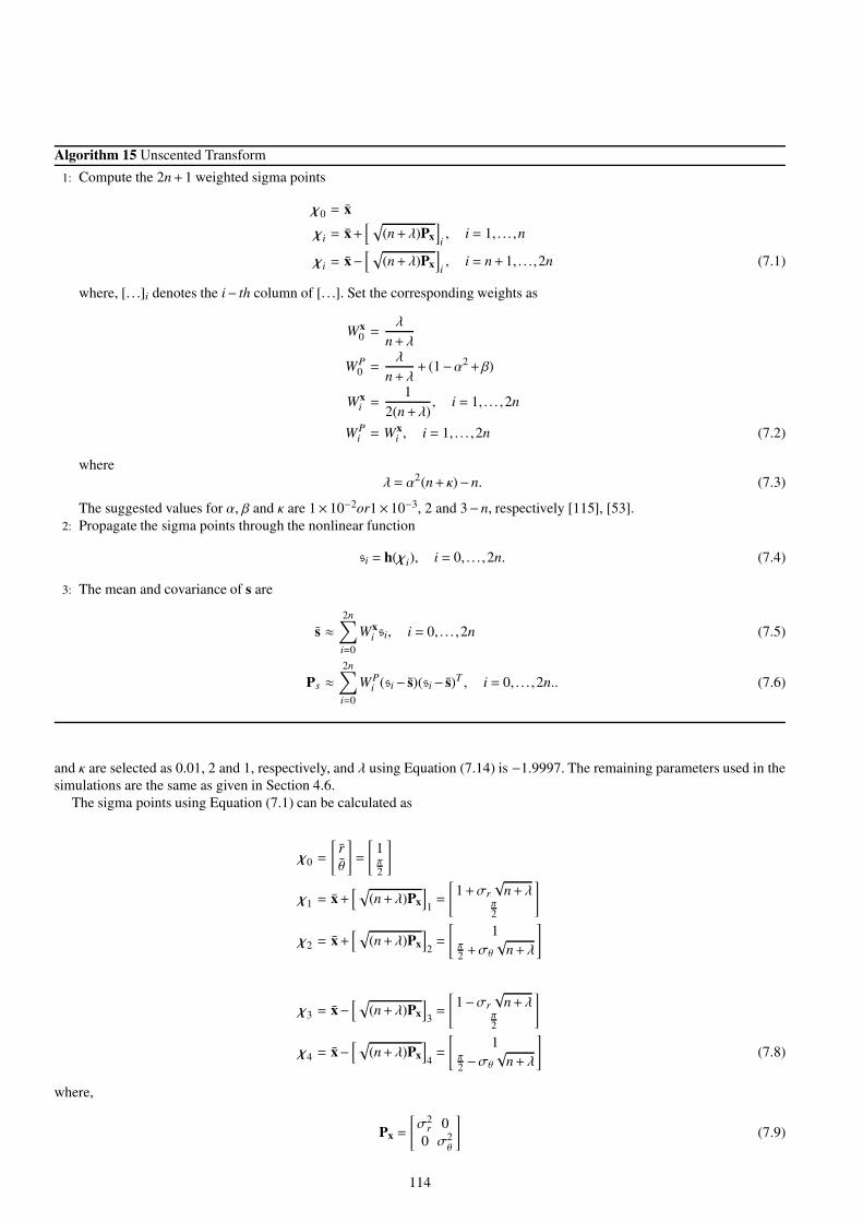
Algorithm 15 Unscented Transform
1: Compute the 2n+1 weighted sigma points
χ0 = x
χi = x+[ √
(n+λ)Px
]i, i = 1, . . . ,n
χi = x−[ √
(n+λ)Px
]i, i = n+1, . . . ,2n (7.1)
where, [. . .]i denotes the i− th column of [. . .]. Set the corresponding weights as
Wx0 =
λ
n+λ
WP0 =
λ
n+λ+ (1−α2+β)
Wxi =
1
2(n+λ), i = 1, . . . ,2n
WPi = Wx
i , i = 1, . . . ,2n (7.2)
where
λ = α2(n+ κ)−n. (7.3)
The suggested values for α, β and κ are 1×10⁻²or1×10−3, 2 and 3−n, respectively [115], [53].
2: Propagate the sigma points through the nonlinear function
si = h(χi), i = 0, . . . ,2n. (7.4)
3: The mean and covariance of s are
s ≈2n∑
i=0
Wxi si, i = 0, . . . ,2n (7.5)
Ps ≈2n∑
i=0
WPi (si− s)(si− s)T , i = 0, . . . ,2n.. (7.6)
and κ are selected as 0.01, 2 and 1, respectively, and λ using Equation (7.14) is −1.9997. The remaining parameters used in the
simulations are the same as given in Section 4.6.
The sigma points using Equation (7.1) can be calculated as
χ0 =
[r
θ
]=
[1π2
]
χ1 = x+[√
(n+λ)Px
]1=
[1+σr
√n+λ
π2
]
χ2 = x+[√
(n+λ)Px
]2=
[1
π2+σθ
√n+λ
]
χ3 = x−[√
(n+λ)Px
]3=
[1−σr
√n+λ
π2
]
χ4 = x−[√
(n+λ)Px
]4=
[1
π2−σθ
√n+λ
](7.8)
where,
Px =
[σ2
r 0
0 σ2θ
](7.9)
114

The corresponding weights are
Wx0 =
λ
n+λ= −6665.66 (7.10)
WP0 =
λ
n+λ+ (1−α2+β) = −6662.66 (7.11)
Wx1 = Wx
2 =Wx3 =Wx
4 = 1666 (7.12)
WP1 = WP
2 =WP3 =WP
4 = 1666 (7.13)
where
λ = α2(n+ κ)−n= −1.9997. (7.14)
The transformed sigma points using Equation (7.4) are
s0 = h(χ0) = h
([r
θ
])=
[0
1
]
s1 = h(χ1) = h
([1+σr
√n+λ
π2
])=
[0
1+σr
√(n+λ)
]
s2 = h(χ2) = h
([1
π2+σθ
√n+λ
])=
cos
(π2+σθ
√(n+λ)
)
sin(π2+σθ
√(n+λ)
)
s3 = h(χ3) = h
([1−σr
√n+λ
π2
])=
[0
1−σr
√(n+λ)
]
s4 = h(χ4) = h
([1
π2−σθ
√n+λ
])=
cos
(π2−σθ
√(n+λ)
)
sin(π2−σθ
√(n+λ)
) . (7.15)
Once the sigma points and its corresponding weights, and the transformed sigma points, have been obtained, the mean and
covariance of s can be calculated as
s ≈4∑
i=0
Wxi si (7.16)
Ps ≈4∑
i=0
WPi (si− s)(si− s)T . (7.17)
A similar simulation scenario as that given in Section 4.6 is repeated with the unscented transformation and the corresponding
results are shown in Figure 7.1. The mean and covariance of the unscented transformation along with the true and linearised ones
are shown in Figure 7.1. It is very hard to see the true mean as it is hidden behind the unscented transform. The true, linearised
and unscented transformation means are located at (0,0.9798), (0,1) and (0,0.9797), respectively. The error covariances for
true, linearised and unscented transformation are
[0.1991 0
0 0.0213
],
[0.2015 0
0 0.0115
]and
[0.2015 0
0 0.0310
]. (7.18)
The uncertainty ellipse using the unscented transformation is comparatively unbiased as compared to that of the linearised
uncertainty ellipse. It can also be seen that the uncertainty ellipse for the unscented transformation given in Figure 7.1 does not
match with that of the true ellipse along the y-axis. One of the reasons for this mismatch is due to the negative λ. The unscented
transform response can be further improved by tuning α, β and κ.
7.2.2 Unscented Kalman filter
The unscented Kalman filter (UKF) is a recursive filter based on the unscented transformation. In Section 7.2.1, the advantages
of the unscented transformation over the linearisation approximation were demonstrated. The unscented transformation is the
backbone of the UKF.
Consider the discrete-time process and measurement models given by
115

−0.4 −0.2 0 0.2 0.40.92
0.94
0.96
0.98
1
1.02
x
y
true
linearised
unscented
Fig. 7.1: 2000 random measurements are generated with range and bearings, which are uniformly distributed between ±0.02
and ±20. These random points are then processed through the nonlinear polar to cartesian coordinate transformation and are
shown as ∗. The true, linearised and unscented transformation means are represented by •, and , respectively. True, linearised
and unscented transformation uncertainty ellipses are represented by solid, dotted and dashed-dotted lines, respectively.
xk = f(xk−1,uk−1)+wk−1 (7.19)
zk = h(xk)+vk, (7.20)
.
Similar to the extended Kalman filter (EKF) and many other filters, UKF can also be expressed in two stages, prediction and
measurement update stages, and is briefed in Algorithm 16. For more details on UKF, please see, for example [104] and [53].
116
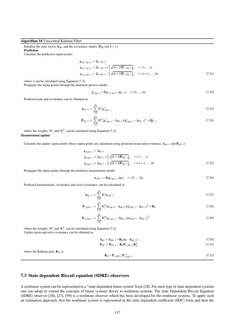
Algorithm 16 Unscented Kalman Filter
Initialise the state vector, x0|0, and the covariance matrix, P0|0 (set k = 1)
Prediction
Calculate the prediction sigma points
χ0,k−1|k−1 = xk−1|k−1
χi,k−1|k−1 = xk−1|k−1 +[ √
(n+λ)Pk−1|k−1
]i, i = 1, . . . ,n
χi,k−1|k−1 = xk−1|k−1 −[ √
(n+λ)Pk−1|k−1
]i, i = n+1, . . . ,2n (7.21)
where λ can be calculated using Equation (7.3).
Propagate the sigma points through the nonlinear process model
χ∗i,k|k−1 = f(χi,k−1|k−1,uk−1), i = 0, . . . ,2n. (7.22)
Predicted state and covariance can be obtained as
xk|k−1 =
2n∑
i=0
W xi χ∗i,k|k−1 (7.23)
Pk|k−1 =
2n∑
i=0
WPi (χ∗i,k|k−1 − xk|k−1)(χ∗i,k|k−1 − xk|k−1)T +Qk−1 (7.24)
where the weights, W xi
and WPi
, can be calculated using Equation (7.2).
Measurement update
Calculate the update sigma points (these sigma points are calculated using predicted mean and covariance, xk|k−1 and Pk|k−1)
χ0,k|k−1 = xk|k−1
χi,k|k−1 = xk|k−1 +[√
(n+λ)Pk|k−1
]i, i = 1, . . . ,n
χi,k|k−1 = xk|k−1 −[√
(n+λ)Pk|k−1
]i, i = n+1, . . . ,2n (7.25)
Propagate the sigma points through the nonlinear measurement model
zi,k|k−1 = h(χi,k|k−1,uk), i = 0, . . . ,2n. (7.26)
Predicted measurement, covariance and cross-covariance can be calculated as
zk|k−1 =
2n∑
i=0
W xi zi,k|k−1 (7.27)
Pzz,k|k−1 =
2n∑
i=0
WPi (zi,k|k−1 − zk|k−1)(zi,k|k−1 − zk|k−1)T +Rk (7.28)
Pxz,k|k−1 =
2n∑
i=0
WPi (χi,k|k−1 − xk|k−1)(zi,k|k−1 − zk|k−1)T (7.29)
where the weights, W xi
and WPi
, can be calculated using Equation (7.2).
Update mean and error covariance can be obtained as
xk|k = xk|k−1 +Kk(zk − zk|k−1) (7.30)
Pk|k = Pk|k−1 −KkPzz,k|k−1KTk (7.31)
where the Kalman gain, Kk, is
Kk = Pxz,k|k−1P−1zz,k|k−1 . (7.32)
7.3 State dependent Riccati equation (SDRE) observers
A nonlinear system can be represented in a “state dependent linear system”form [28]. For such type of state dependent systems
one can adopt or extend the concepts of linear systems theory to nonlinear systems. The state Dependent Riccati Equation
(SDRE) observer [28], [27], [99] is a nonlinear observer which has been developed for the nonlinear systems. To apply such
an estimation approach, first the nonlinear system is represented in the state dependent coefficient (SDC) form and then the
117

observer is synthesized for the state dependent system. One of the main advantages of SDRE observer over other existing
observers/estimators is that there exists infinitely many possible combinations of SDC systems [27], [70]. One can choose the
best possible SDC system as per the problem at hand. Further, the SDRE observer does not need Jacobians during the estimation
process.
Consider the discrete-time, process and measurement models
xk = f(xk−1,uk−1)+wk−1 (7.33)
zk = h(xk)+vk, (7.34)
where, k is the time index showing the current time instant, xk ∈ Rn represents the state vector, uk ∈ Rq is the control input
vector, zk ∈ Rp is the measurement vector, and wk−1 and vk are the process and measurement noises. In this section, the process
and measurement noises are assumed to be Gaussian with zero means and with covariances of Qk−1 and Rk,
wk−1 =N(0,Qk−1)
vk =N(0,Rk),
where,N represents the Gaussian or normal probability distribution.
The nonlinear models in Equations (7.33) and (7.34) can be represented in the state dependent coefficient (SDC) [82] form
as:
xk = F(xk−1)xk−1 +G(xk−1)uk−1 +wk−1 (7.35)
zk = H(xk)xk +vk. (7.36)
Note that the SDC matrices, F, G and H, for nonlinear systems are non-unique.
Consider a simple example, where the nonlinear plant dynamics is given by:
xk = f(xk−1) =
[x2,k−1
x21,k−1
]. (7.37)
The SDC form of Equation (7.37) can be written as:
fk−1 = F1(xk−1)xk−1 = F2(xk−1)xk−1 = F3(xk−1)xk−1 = . . ., where the SDC matrices are:
F1(xk−1) =
[0 1
x1,k−1 0
],
F2(xk−1) =
[ x2,k−1
x1,k−10
x1 0
],
F3(xk−1) = λF1(xk−1)xk−1 + (1−λ)F2(xk−1).
A similar example was considered in [10]. Different parameterisations can be obtained for different values of “λ” in the
interval [0,1], which satisfies the convexity of the chosen parametrisation. Similarly, different combinations of the SDC mea-
surement matrices, Hi, and the state vector, xk, can yield the same h(xk), like H1(xk)xk =H2(xk)xk =H3(xk)xk = h(xk).
As the SDC matrices are non-unique, before designing the SDRE observer (or SDRE controller), one should make sure that
the state-dependent observability matrix (or the state-dependent controllability matrix) is of full rank [10].
Similar to the Kalman filter, the SDRE observer can be formulated in prediction and measurement update stages [50]. The
predicted state, xk|k−1, and positive definite matrix, Pk|k−1, can be written as:
xk|k−1 = f(xk−1|k−1,uk−1) (7.38)
Pk|k−1 = F(xk−1|k−1)Pk−1|k−1F(xk−1|k−1)T +Qk−1. (7.39)
The updated state, xk|k, and positive definite matrix, Pk|k, are:
xk|k = xk|k−1 +Kk[zk −H(xk|k−1)] (7.40)
Pk|k = (In −KkH(xk|k−1))Pk|k−1, (7.41)
where, In denotes the identity matrix of dimension n×n and the SDRE observer gain is:
118

Kk = Pk|k−1H(xk|k−1)T[H(xk|k−1)Pk|k−1H(xk|k−1)T +Rk
]−1. (7.42)
It can be noted that the matrices Pk|k−1 and Pk|k satisfy the Riccati recursion and are state dependent. At first glance, the above
formulation looks similar to that of the EKF; but actually it is not. The main difference between the SDRE observdr and the
EKF is the way in which the matrices F(xk−1|k−1)) and H(xk|k−1) are defined. In the SDRE observer they are the parameterised
SDC matrices and for the EKF they are the Jacobians of the process and measurement models. The SDRE filter avoids the
evaluation of Jacobians and hence avoids the errors introduced by the truncation of Taylor series. It is interesting to note that
different parameterisations in the SDRE filter may yield different results [74].
7.4 SDRE Information Filter
This section presents the formulation for the SDRE information filter (SDREIF). The SDRE filter and the extended information
filter (EIF) are to be fused to form the SDREIF, which will have the benefits of both filters. The SDREIF is a derivative free
(Jacobian free) filter like the SDRE filter, and like the EIF, it is handy to deal with the multi-sensor state estimation. Similar
to the information filter, the SDREIF is developed in the information domain, where the information vector and information
matrix are propagated.
Consider the discrete-time process and measurement models given in Eqs. (7.33) and (7.34), and its SDC form in Eqs. (7.66)
and (7.67). The predicted information vector, yk|k−1, and the inverse of the positive definite matrix, Yk|k−1 = P−1k|k−1
, for the
SDREIF are:
yk|k−1 = Yk|k−1xk|k−1 (7.43)
Yk|k−1 =[F(xk−1|k−1)Y−1
k−1|k−1F(xk−1|k−1)T +Qk−1
]−1, (7.44)
where
xk|k−1 = f(xk−1|k−1,uk−1). (7.45)
It can be seen that the predicted information vector in Eq. (7.43) is the same as that of the EIF, but the expression for Pk|k−1
is different. In the EIF, the updated information matrix is the function of the Jacobian, ∇fx, whereas in the SDREIF the ∇fx is
replaced by the SDC F(xk−1).
The updated information vector, yk|k, and Yk|k are:
yk|k = yk|k−1 + ik (7.46)
Yk|k = Yk|k−1 + Ik. (7.47)
The information vector contribution, ik, and its associated information matrix contribution, Ik, are
ik = H(xk|k−1)T R−1k
[νk +H(xk|k−1)xk|k−1
](7.48)
Ik = H(xk|k−1)T R−1k H(xk|k−1) (7.49)
where the measurement residual, νk, is
νk = zk −H(xk|k−1). (7.50)
7.4.1 SDREIF in multi-sensor state estimation
One of the main advantages of the state estimation in the information domain is its ability to easily deal with the multi-
sensor state estimation [83], [11]. In the update stage, the information from various sensors can be easily fused [83], [11]. The
prediction step for the SDREIF multi-sensor state estimation is the same as that of the SDREIF (with a single sensor). In the
update stage, the data from different sensors are fused for an efficient and reliable estimation [93].
Let the different sensors used for the state estimation be given by
z j,k = h j,k(x j,k)+v j,k; j = 1,2, ...D, (7.51)
where ‘D’ is the number of sensors. The parameterised SDC form for the multi-sensor models can be written as:
119
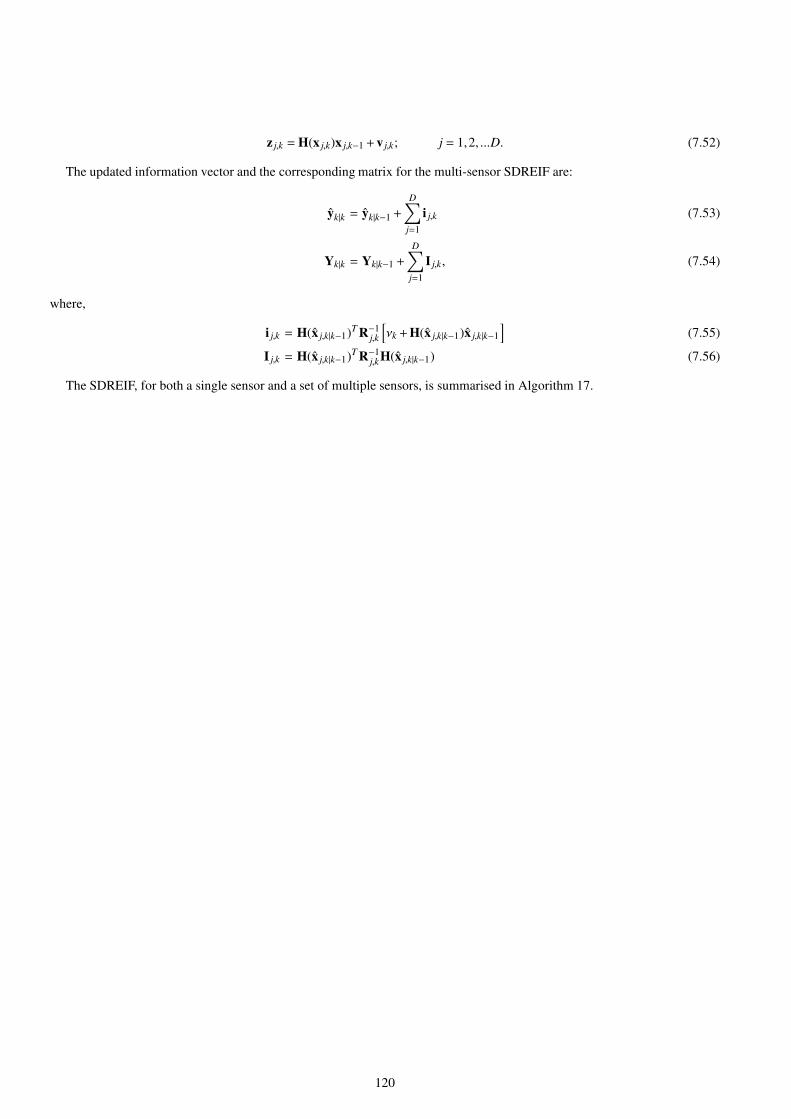
z j,k =H(x j,k)x j,k−1 +v j,k; j = 1,2, ...D. (7.52)
The updated information vector and the corresponding matrix for the multi-sensor SDREIF are:
yk|k = yk|k−1 +
D∑
j=1
i j,k (7.53)
Yk|k = Yk|k−1 +
D∑
j=1
I j,k, (7.54)
where,
i j,k = H(x j,k|k−1)T R−1j,k
[νk +H(x j,k|k−1)x j,k|k−1
](7.55)
I j,k = H(x j,k|k−1)T R−1j,kH(x j,k|k−1) (7.56)
The SDREIF, for both a single sensor and a set of multiple sensors, is summarised in Algorithm 17.
120

Algorithm 17 State Dependent Riccati Equation Information Filter (SDREIF)
State Dependent Coefficient Form:
Use paramerisation to bring the nonlinear process and measurement models in to the below SDC form:
xk = F(xk−1)xk−1 +G(xk−1)uk−1 +wk−1
zk = H(xk)xk−1 +vk .
Prediction:
Initialise the information vector, yk−1|k−1 , and the associated matrix, Yk−1|k−1; by setting k = 1.
The predicted information vector and the associate matrix are:
yk|k−1 = Yk|k−1xk|k−1
Yk|k−1 =[F(xk−1|k−1)Y−1
k−1|k−1F(xk−1|k−1)T +Qk−1
]−1,
where,
xk|k−1 = f(xk−1|k−1 ,uk−1).
Measurement Update:
Evaluate the information vector contribution and its associated information matrix
ik = H(xk|k−1)T R−1k
[νk +H(xk|k−1)xk|k−1
](7.57)
Ik = H(xk|k−1)T R−1k H(xk|k−1) (7.58)
where, the measurement residual, νk, is
νk = zk −H(xk|k−1). (7.59)
The updated information vector and the corresponding matrix are
yk|k = yk|k−1 + ik
Yk|k = Yk|k−1 + Ik .
For the state estimation with multiple sensors, the updated information vector and the corresponding matrix are:
yk|k = yk|k−1 +
D∑
j=1
i j,k (7.60)
Yk|k = Yk|k−1 +
D∑
j=1
I j,k, (7.61)
where,
i j,k = H(x j,k|k−1)T R−1j,k
[νk +H(x j,k|k−1)x j,k|k−1
](7.62)
I j,k = H(x j,k|k−1)T R−1j,kH(x j,k|k−1) (7.63)
Recovery of State and the Corresponding Matrix:
The state and the corresponding positive definite matrix can be recovered as:
xk|k =Yk|k\yk|k (7.64)
Pk|k =Yk|k\In (7.65)
where In is the state vector sized identity matrix.
121

7.5 PMSM case revisited
The state estimation of a two phase permanent magnet synchronous motor (PMSM) was considered in Chapter 6 and is to be
reconsidered here by using the state dependent Riccati equation information filtering approach. The state vector of the PMSM
are, [ia, ib,ω,θ]T . The inputs to the PMSM are the voltages, u1,k and u2,k. It is assumed that the first two states, ia and ib, are
available for direct measurement and the remaining two states, ω and θ, are to be estimated.
The discrete-time nonlinear model of PMSM is [104], [18]
ia,k+1
ib,k+1
ωk+1
θk+1
=
ia,k +Ts(−RL
ia,k +ωλL
sinθk +1L
u1,k)
ib,k +Ts(−RL
ib,k − ωλL
cosθk +1L
u2,k)
θk +Ts(− 3λ2J
ia,k sinθk +3λ2J
ib,k cosθk − Fωk
J)
θk +Tsωk
the outputs and inputs are [y1,k
y2,k
]=
[ia,kib,k
],
[u1,k
u2,k
]=
[sin(0.002πk)
cos(0.002πk)
].
The following parameters are used for the simulations [104], [20]: R = 1.9Ω, λ=0.1, L = 0.003H, J = 0.00018, F = 0.001
and Ts = 0.001 s. It is assumed that the plant and measurement models are excited with the additive Gaussian noises.
The first step to implement the SDREIF is to bring the process and measurement equations in the SDC form. In this section
the following SDC form is to be used:
xk = F(xk−1)xk−1 +G(xk−1)uk−1 +wk−1 (7.66)
zk = H(xk)xk−1 +vk. (7.67)
where,
F(xk−1) = I4+Ts
−RL
0 λL
sinθk 0
0 −RL
λL
cosθk 0
− 32λJ
sinθk32λJ
cosθk − BJ
0
0 0 1 0
G(xk−1) =
1L
0
0 1L
0 0
0 0
H(xk) =
[1 0 0 0
0 1 0 0
]
Two groups of simulations have been performed on the PMSM to analyse the proposed SDREIF. The first group are simulated
with a single set of sensors and the second group of simulations are performed with two sets of sensors. In the first group of
simulations, the covariance of the process and measurement noise are:
Q =
11.1111 0 0 0
0 11.1111 0 0
0 0 0.0025 0
0 0 0 1×10⁻⁶
, R = 1×10⁻⁴I2
The initial information vector is selected fromN([
1 1 1 1]T,I4
).
It was further assumed that the first sensor (ia measurement) and the second sensor (ib measurement) are faulty from 0.5 s-
0.8 s and 2 s to 2.3 s, respectively. In this case study, the term ‘faulty’ means the sensor only outputs zero measurements during
this condition. Figure 7.2 shows the plots of actual and measured data; where it was assumed that the first and second sensors
are faulty for some time periods. In the first group of simulations, a single set of sensors are used to measure the currents, ia and
ib; andω and θ are estimated using the SDREIF given in Section 7.4 and for the second group of simulations, two sets of sensors
are used and the procedure given in the Section 7.4.1 is used. For the multi-sensor state estimation, the first set of sensors are
the same as that of the single sensor state estimation; the noise covariance of the second set of sensors is: R2 = 4×10⁻⁶I2. The
corresponding results are depicted in Figure 7.3. It can be seen that the SDREIF using a single set of sensors are not capable
to handle the faulty sensors; whereas the multi-sensor SDREIF can handle it efficiently. It is interesting to note that, during the
122

faulty measurements also the multi-sensor SDREIF could able to keep the error within an acceptable bound. The error plots
using the single-set and multi-set of sensors are shown in Figure 7.4.
0 0.5 1 1.5 2 2.5 3 3.5 4 4.5 5−0.4
−0.2
0
0.2
0.4
Time (s)
x1 (
Am
ps)
Acutal Measured
0 0.5 1 1.5 2 2.5 3 3.5 4 4.5 5−0.4
−0.2
0
0.2
0.4
Time (s)
x2 (
Am
ps)
Acutal Measured
Fig. 7.2: Actual and measured data.
7.6 Filter robustness consideration
All engineering control systems are operating in the real environment, and are subject to uncertainties. Therefore, a practically
useful control system must have the ability to deal with uncertainties. This is so called “robustness” property. This section
will first introduce what kind of uncertainties commonly affect the behaviour of a control system, and then will consider the
robustness of state estimators (filters).
7.6.1 Uncertainties and robustness requirement
It is well understood that uncertainties are unavoidable for a real control system in its operation. The uncertainty possibly
affecting a control system can be classified in two categories: dynamic perturbations and signal disturbances. The former
represent the discrepancy between the mathematical model used for design and the actual dynamics of the system in operations.
A mathematical model of any real system is always just an approximation of the true, physical reality of the system dynamics.
Typical sources of the discrepancy include unmodelled (usually high-frequency) dynamics, neglected nonlinearities in the
modelling, effects of deliberately reduced-order models, and system-parameter variations due to environmental changes and
torn-and-worn consequences. These modelling errors may adversely affect the stability and performance of a control system.
The latter include input and output disturbances (such as a gust on an aircraft), sensor noises and actuator noises, etc. Concerning
the subject of this book, i.e. design of state estimators, signal disturbances are mainly considered to be the accuracy and
availability of sensory data (plant input and output measurements) to the estimators (filters).
Detailed exposure of control systems robustness can be found in many resources, for example, the book by Gu, Petkov and
Konstantinov [43].
A control system being robust indicates that it remains (internally) stable and keeps up certain performance level in the
presence of uncertainties. For a state estimator, it is required to perform nearly normally when the dynamics of the underlying
control system is not known exactly during the estimator design and when occasionally the sensory data are inaccurate or do
not arrive in time.
123
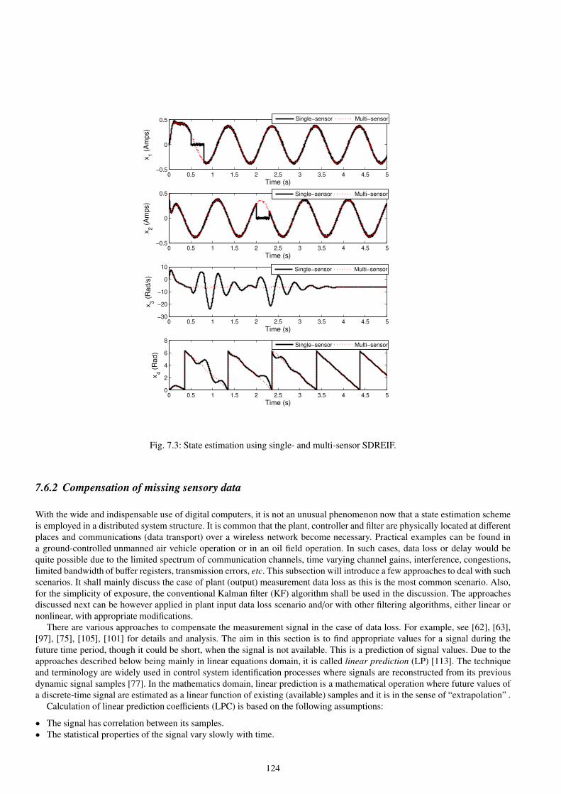
0 0.5 1 1.5 2 2.5 3 3.5 4 4.5 5−0.5
0
0.5
Time (s)
x1 (
Am
ps)
Single−sensor Multi−sensor
0 0.5 1 1.5 2 2.5 3 3.5 4 4.5 5−0.5
0
0.5
Time (s)
x2 (
Am
ps)
Single−sensor Multi−sensor
0 0.5 1 1.5 2 2.5 3 3.5 4 4.5 5−30
−20
−10
0
10
Time (s)
x3 (
Ra
d/s
)
Single−sensor Multi−sensor
0 0.5 1 1.5 2 2.5 3 3.5 4 4.5 50
2
4
6
8
Time (s)
x4 (
Ra
d)
Single−sensor Multi−sensor
Fig. 7.3: State estimation using single- and multi-sensor SDREIF.
7.6.2 Compensation of missing sensory data
With the wide and indispensable use of digital computers, it is not an unusual phenomenon now that a state estimation scheme
is employed in a distributed system structure. It is common that the plant, controller and filter are physically located at different
places and communications (data transport) over a wireless network become necessary. Practical examples can be found in
a ground-controlled unmanned air vehicle operation or in an oil field operation. In such cases, data loss or delay would be
quite possible due to the limited spectrum of communication channels, time varying channel gains, interference, congestions,
limited bandwidth of buffer registers, transmission errors, etc. This subsection will introduce a few approaches to deal with such
scenarios. It shall mainly discuss the case of plant (output) measurement data loss as this is the most common scenario. Also,
for the simplicity of exposure, the conventional Kalman filter (KF) algorithm shall be used in the discussion. The approaches
discussed next can be however applied in plant input data loss scenario and/or with other filtering algorithms, either linear or
nonlinear, with appropriate modifications.
There are various approaches to compensate the measurement signal in the case of data loss. For example, see [62], [63],
[97], [75], [105], [101] for details and analysis. The aim in this section is to find appropriate values for a signal during the
future time period, though it could be short, when the signal is not available. This is a prediction of signal values. Due to the
approaches described below being mainly in linear equations domain, it is called linear prediction (LP) [113]. The technique
and terminology are widely used in control system identification processes where signals are reconstructed from its previous
dynamic signal samples [77]. In the mathematics domain, linear prediction is a mathematical operation where future values of
a discrete-time signal are estimated as a linear function of existing (available) samples and it is in the sense of “extrapolation” .
Calculation of linear prediction coefficients (LPC) is based on the following assumptions:
• The signal has correlation between its samples.
• The statistical properties of the signal vary slowly with time.
124

0 0.5 1 1.5 2 2.5 3 3.5 4 4.5 5−0.4
−0.2
0
0.2
0.4
Time (s)
Err
or
in x
1 (
Am
ps)
Single−sensor Multi−sensor
0 0.5 1 1.5 2 2.5 3 3.5 4 4.5 5−0.2
0
0.2
0.4
0.6
Time (s)
Err
or
in x
2 (
Am
ps)
Single−sensor Multi−sensor
0 0.5 1 1.5 2 2.5 3 3.5 4 4.5 5−20
−10
0
10
20
Time (s)
Err
or
in x
3 (
Ra
d/s
)
Single−sensor Multi−sensor
0 0.5 1 1.5 2 2.5 3 3.5 4 4.5 5−10
−5
0
5
10
Time (s)
Err
or
in x
4 (
Ra
d)
Single−sensor Multi−sensor
Fig. 7.4: Error plots using single- and multi-sensor SDREIF.
If the above assumptions are satisfied, the future values, or the current value depending on the definition of the index k, of the
signal can be reconstructed [25]. In the context considered, the scheme can be represented by the following equation:
zk =
n∑
j=1
α jzk− j +
N∑
i=0
biuk−i (7.68)
where zk denotes the estimated value at the time instant k; and, α j = [α1,α2, ....αn] are parameters of the algorithm which are
so-called Linear Prediction parameters of measurement (output) and bi = [b1,b2, ....bn] are the parameters of the input. Based
on various combinations, one might define different prediction schemes in relation to the linear prediction method, e.g. Au-
toregressive (AR) Model, Moving Average (MA) Model, Autoregressive Moving Average (ARMA) Model etc., see [114] for
further details. Obviously, the value of linear prediction coefficients (LPC) and the orders of the two terms in the right side of
(7.68) affects the result of compensation greatly. That will be discussed a bit further later in this chapter.
Zero Kalman gain matrix
When the measurement is not available, a straightforward idea is just to ignore it and to calculate the “measurement” directly
from the system output equation with newly available predicted state instead of true state. That is, in the Kalman filter algorithm,
one assumes that zk =Hkxk|k−1. That leads to the residual (innovation) vector νk to be zero, i.e. the “measurement” equals the
predicted output. It is equivalent to setting the Kalman filter gain matrix Kk to be zero consequently in the updating stage. As
soon as the measurement becomes available, the calculations go back to the normal procedure in the Kalman filter algorithm.
Despite of fast calculation, simpler structure and no need of storing observations, there are quite a few drawbacks associated
with this approach for the loss of observation. In practice, Kalman filter procedure with zero gain matrix may diverge and it
125

is likely to happen that the error covariance could exceed the bounded error limits provided [75]. Another shortcoming is that
when the system measurement (observation) is resumed after the loss period, one can see a sharp spike phenomenon in the
estimation error, a kind of bump switch in control engineering terminology. This is because the Kalman filter gain is set to zero
when data loss is occurred; however, when observation is repossessed, the filter gain will surge to a high value and then attain
the steady state value in order to compensate loss impact [64]. This feature consequently results in a sudden peak to reach the
normal trajectory of the estimated state which is an undesirable behaviour of the estimation algorithm. Another serious short-
coming associated with zeroing Kalman gain matrix approach is that it takes a far long time to regain the values of estimated
states and covariance within satisfactory bands afterwards. In theory, it will take infinite time to retrieve the steady state values,
due to the recursive nature of the filtering algorithm operations.
Zero-order hold (ZOH)
If the filter parameters are selected as n = 1, α = 1 and without the input terms in Equation (7.68), the compensated observa-
tion vector will be retranslated as
zk = zk−1 = Hxk−1 + vk−1
In the literature, the above scheme is known as the Zero-order Hold (ZOH) method, due to the fact that the last observation
is held to provide the measurement update step for the predicted state and error covariance. The ZOH method can be a useful
approach for systems with sufficiently slow measurement samples (such as ship dynamics, commercial airplanes, etc.). How-
ever, it is prone to fail in the reconstruction of the given signal if the sampling frequency of sensors measurements are high
(such as with jet fighters, UAVs, etc.). It also will not work when the data loss continues to a relatively long period of time.
First-order hold (FOH)
If it is assumed that n = 2 and αi = [α1,α2], and without the input terms in Equation (7.68), the following will be obtained
zk = α1zk−1 +α2zk−2 (7.69)
The scheme is known as the First-order Hold (FOH) approach. When α1 = α2 = 0.5, i.e. the two weights are set equal, it will
become
zk =zk−1 + zk−2
2
As it can be seen, in the above LP approaches, one does not require to compute the parameters in relation to the linear
prediction system. Obviously, these two coefficients can be set differently to form weighted observations. That is to view the
previous two measurements, (zk−1 and zk−2), with different significance on forming the current, estimated measurement. Usually
and logically, the closer data would have more impact on the estimated measurement and hence the bigger weight to be set.
Trend approach
In some applications, one may notice that the observation vector contains a regular pattern in the received data. In such cases,
data missing would not affect the estimation to a high extent while these trends can vary from time to time and from a system
to another [60]. For the sake of easy understanding, and without loss of generality, it is assumed that
zk = zk−1 + [zk−1− zk−2] (7.70)
or
zk+1 = Hxk + νk+ [Hxk+ νk −Hxk−1− νk−1]
= Hxk + νk+ [H∆xk+∆νk]
= H(xk+∆xk)+ (νk+∆νk)
= Hxk+1 + νk+1 (7.71)
where ∆xk = xk − xk−1 and ∆νk = νk − νk−1, xk+1 = xk +∆xk and νk+1 = νk +∆νk.
126

Autoregressive approach (AR)
For n≥ 2 in (7.68) and without the input terms, the approach is termed as Autoregressive (AR) approach in which every (past)
measurement is associated with a weight (coefficient) to form the current measurement(estimation). All the three approaches
above are actually special cases of the Autoregressive approach. Therefore, the measurement equation is written as
zk =1
n
n∑
j=1
zk− j
= H1
n
n∑
j=1
xk− j +1
n
n∑
j=1
νk− j
= Hxk + νk (7.72)
where xk =1
n
n∑
j=1
xk− j and νk =1n
n∑
j=1
νk− j.
Autoregressive moving average approach (ARMA)
The approaches introduced above are all concentrating on the past sensed, or past estimated, measurements. They do not
depend on the input signal to the underlying system, i.e. the second part of the right-hand side of Equation (7.68) is not explored.
The autoregressive moving average (ARMA) approach however does explore the use of the input. With the ARMA approach,
more design freedom, in terms of number of design parameters, is available and may produce better estimation results.
All the design parameters involved in (7.68) can be determined by using some optimisation methods, for example the ones
described in [63]. However, it should be noted that higher order (n and N in (7.68)) does not always imply better estimation
results [25].
7.6.3 Selection of linear prediction coefficients and orders
In this subsection a method to select the linear prediction coefficients and order of an autoregressive model used in observation
data loss compensation is to be introduced. This method and the case study followed in the next subsection were firstly proposed
and considered in [63, 65]. Interested readers can find more details in these references. However, please note some notations
and definitions of nomenclature have been changed to suit those used in this book.
It is assumed that a general AR-series is mathematically modelled by
zk = c+
n∑
j=1
α jzk− j + ξk (7.73)
where zk is the signal which is to be reconstructed based on previous sensed data and hence it is referred as compensated output
signal. To carry out the signal prediction, “optimal” values of α j are to be computed through the auto-correlation function using
Yule-Walker equation [25]:
γm =
n∑
j=1
α jγm− j +σ2δm (7.74)
where δm is the Kroncker delta, that is
δm =
1; if m = 0
0; otherwise(7.75)
In Equation (7.73) c is a constant (normally the mean of the signal) and ξk is a noise input signal. If the input is a white
noise, the model is referred to as an “All-Pole Infinite Impulse Response (IIR)” filter, where n is the filter order. It is assumed in
this book that the noise involved is white and unmeasurable, and consequently c and the noise term will vanish in the equation.
Hence it is supposed
127

zk =
n∑
j=1
α jzk− j (7.76)
The computation of “optimal” values of α j and the order of the linear prediction (LP) filter, n, are critical for the estimation
problem with loss of measurements. It is worthwhile to note that a large number of previous data does not always guarantee an
optimal prediction of the missing data [25].
In general, there are two types of processes: First- Stationary Process where the joint probability distribution of the process
does not change with time shifting; Secondly- Non-stationary Process, i.e. it does change with time. In this book, only the
stationary processes are considered. In addition, it is assumed that the process is Wide-Sense Stationary (WSS), i.e. the mean
and variance are time independent [45], which is shown as
E[z(t)
]= mz(t) = mz(t+ τ) ∀ τ ∈ R &
E[z(t1)z(t2)
]= E
[z(t1+ τ)z(t2+ τ)
]
= Rz(t1, t2) ∀ τ ∈ R (7.77)
The linear prediction parameters, the coefficients and order, define the contributions of previous observation made for re-
constructing the missing data. This can be viewed from the data autocorrelation standpoint. The output error generated by this
compensated observation vector is
ez(k) = zk − zk (7.78)
The residual related cost function can be defined based on the output error in the form of
Jk = E[ez(k)T ez(k)
](7.79)
Optimal values of the LP parameters, α j can be found by minimizing the above cost function, Jk. That is,
∂Jk
∂αi
=∂
∂α j
E[ez(k)T ez(k)
]
= E[∂(ez(k)T ez(k)
)
∂αi
]
= E[∂Jk
∂zk
∂zk
∂αi
](7.80)
Also, from Equations (7.78) and (7.79)
∂Jk
∂zk
= 2[ez(k)T ]
= 2[zk − zk
]T(7.81)
By differentiating zk with regard to αi, one can have
∂zk
∂αi
= zk−i (7.82)
In order to minimize the cost function, Jk, from Equation (7.80), one should first have
∂Jk
∂αi
= 0 (7.83)
From Equation (7.80) through Equation (7.82),
E[2(zk − zk
)T]zk−i = 0
E[zT
k zk−i
]−E
[zT
k zk−i
]= 0
By substituting Equation (7.76), one will have
128

n∑
j=1
α jE[zT
k− jzk−i
]= E[zT
k zk−i] (7.84)
which can be simplified as
RγAα = rγ (7.85)
or
Aα = R−1γ · rγ (7.86)
where
Rγ =
Rγ(0) Rγ(1) Rγ(2) · · · Rγ(n−1)
Rγ(1) Rγ(0) Rγ(1) · · · Rγ(n−2)
Rγ(2) Rγ(1) Rγ(0) · · · Rγ(n−3)
.
.
....
.
.
.. . .
.
.
.
Rγ(n−1) Rγ(n−2) Rγ(n−3) · · · Rγ(0)
(7.87)
Aα =[α1 α2 α3 · · · αn
]T(7.88)
rγ =[rγ(1) rγ(2) rγ(3) · · · rγ(n)
]T(7.89)
E[zT
k− jzk−i
]=
Rγ(0), if j = i
Rγ(| j− i|), if j , i
(7.90)
and
rγ(i) = E[zT
k zk−i
](7.91)
The LP filter optimal values will be calculated through solving Equation (7.86). It is worthwhile to notice that the complexity
of the LP filter is directly related to the calculation burdensome of Equation (7.86) which depends heavily on the size of matrix
Rγ, or the order of LP filter. Higher orders of an LP filter does not necessarily yield a better reconstruction of a lost signal as
mentioned earlier. It is therefore useful to address the “optimal order” of the LP filter next.
As being discussed earlier, the higher orders of LP filter does not guarantee a better reconstruction of signal, which makes
the selection process of the order of an LP filter more critical. Toward this end, it is essential to propose some easy-to-implement
approaches in order to provide “good” values of the LP filter order. Among a few alternative algorithms, the following straight-
forward approaches are found “better” than other methods along with an assumption required which is listed below.
Assumption: To employ these methods, it is assumed that T f ≥ nTs where Ts is the sampling time, T f is the starting time
of loss of observations (LOOB), and n is the LP filter’s order. This assumption is clearly required due to the fact that the
lost observation requires n signal sample to be reconstructed as of Equation (7.86). This assumption indicates an additional
importance for the selection of appropriate LP order.
Assume that the starting time instant of LOOB to be at time t = k. Having the measurement updated step known at time
instant k− 1, two methods are to be proposed both of which are aimed at yielding an optimal order of the LP filter. The first
method is detailed in Algorithm 18.
129

Algorithm 18 Selection of the LP filter order (first method)
Compute em(k−1) = max (ei), where ei = xi − xi for
i = 1,2, ....k−1.Initialization j = 1, Compute Rγ and rγ through Equations (7.90) and (7.91) respectively.
Recursion: j = 2....M
Obtain z through Equation (7.76)
Calculate measurement updated state c xk
based on this Compensated Observations
Compute e j(k) = xk − xk.
Check Is e j(k) ≤ em(k−1)
Yes n←− j : Order of the LP Filter
Else j←− j+1
Repeat Step 4
It is worthwhile to emphasise that the autocorrelation of a function indicates in fact the similarity of the signal with its timely
separated function. Hence, for a well-established Rγ, the above factors of Rγ are ranging from +1, for a perfect correlation, to
-1, for a fully anti-correlated case. Hence the maximum correlation would be for zero time shift.
Generally speaking, the autocorrelation function for two different time shifts p and q will be
γ(p,q) =E[(zk−p−µp)(zk−q −µq)
]
σpσq
(7.92)
Due to the property of WSS (7.77), for the same time shifts (p = q), the autocorrelation would result in
γ(p, p) = Rγ(p) =E[(zk−p−µ)(zk−p−µ)
]
σk−pσk−p
=E[(zk−p−µ)(zk−p−µ)
]
σ2
= 1 (7.93)
for any non-zero variance σ value. It is also noticed that the longer the time shift is, the lesser correlation will be resulted.
Hence, the following autocorrelation-related inequality can be readily inferred:
Rγ(n) ≥ · · ·Rγ( j) ≥ · · · ≥ Rγ(1) ≥ Rγ(0) (7.94)
The inequality criteria of Equation (7.94), most likely, leads to a simplest routine in choosing the order of LP filter. Neverthe-
less, one might propose alternative approaches to tackle the problem of order selection process. To this end, another algorithm
is to be introduced which is based on the above inequality to extract the LP order and is summarized in Algorithm 19.
Algorithm 19 Selection of the LP filter order (second method)
Select γth.
Recursion j = 1,2, · · ·MCompute γ( j) using Equation (7.92)
Check: Is γ( j) ≤ γth,
Yes Stop further computation of γ j and
Select order of LP filter (n← j)
Else update j←− j+1
Repeat Step 3
7.6.4 A case study
In this section, the Mass-Spring Damper (MSD) system shown in Figure 7.5 is to be modelled first. This is a slightly modified
version of the MSD system analysed in [37]. Four states are related with this system, out of which only one is measured through
a noisy sensor. Initially the conventional Kalman filter is implemented and tested with no loss of data (normal operation). There-
after, an (artificial) fault is introduced in the sensor due to which the sensor readings are not available for the duration of 2.3
to 3.3 seconds. The compensation with zero Kalman gain matrix and then the AR compensation algorithm with optimal linear
130

prediction coefficients introduced earlier will be applied in such scenarios to see the data compensation results .
Model of Mass-Spring-Damper (MSD) system
The system under study here is a mass-spring-damper (MSD) system, whose continuous-time dynamics are described as
follows:
x(t) = Ax(t)+Bu(t)+ Lw(t)
zk = Cxk + vk (7.95)
The state vector
xT (t) = [ x1(t) x2(t) x1(t) x2(t) ] (7.96)
is composed of displacements and speed of the two masses in Fig 7.5.
A =
0 0 1 0
0 0 0 1k1
m1
k1
m1− b1
m1b1m1
k1m2− k1+k2
m1
b1m2− b1+b2
m2
(7.97)
BT = [ 0 0 1m1
0 ] (7.98)
C = [ 0 1 0 0 ] (7.99)
L = [ 0 0 0 3 ] (7.100)
The known parameters are m1 = m2 = 1, k1 = 1, k2 = 0.15, b1 = b2 = 0.1 and the sampling time is Ts = 1 msecs. Also, the
MSD plant disturbance and sensor noise dynamics are characterized as
Ew(t)
= 0, E
w(t)w(τ)
= Ξδ(t− τ), Ξ = 1 (7.101)
Ev(t)
= 0, E
v(t)v(τ)
= 10−6δ(t− τ) (7.102)
After substituting the above known values, the system matrices are as follows:
A =
0 0 1 0
0 0 0 1
1 1 −0.1 0.1
0.1 −1.15 0.1 −0.2
(7.103)
and
Control
u(t)
x1
k1
x2
k2
m1 m2b1 b2
Fig. 7.5: MSD two cart system.
131
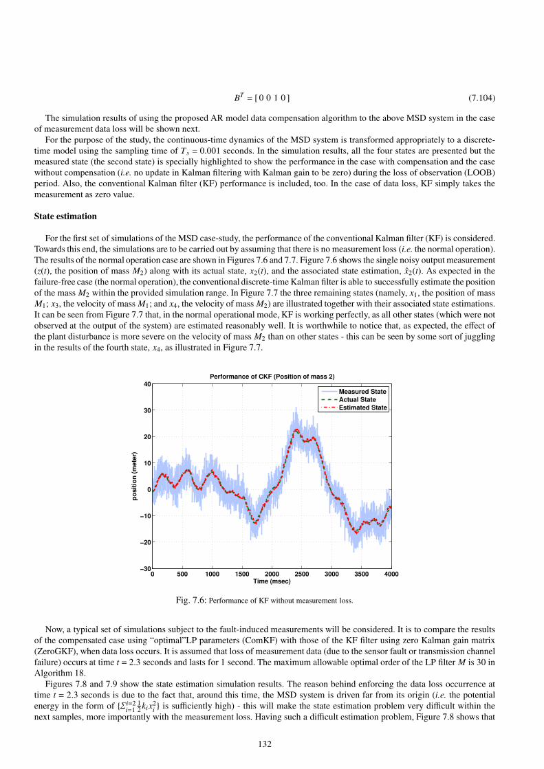
BT = [ 0 0 1 0 ] (7.104)
The simulation results of using the proposed AR model data compensation algorithm to the above MSD system in the case
of measurement data loss will be shown next.
For the purpose of the study, the continuous-time dynamics of the MSD system is transformed appropriately to a discrete-
time model using the sampling time of Ts = 0.001 seconds. In the simulation results, all the four states are presented but the
measured state (the second state) is specially highlighted to show the performance in the case with compensation and the case
without compensation (i.e. no update in Kalman filtering with Kalman gain to be zero) during the loss of observation (LOOB)
period. Also, the conventional Kalman filter (KF) performance is included, too. In the case of data loss, KF simply takes the
measurement as zero value.
State estimation
For the first set of simulations of the MSD case-study, the performance of the conventional Kalman filter (KF) is considered.
Towards this end, the simulations are to be carried out by assuming that there is no measurement loss (i.e. the normal operation).
The results of the normal operation case are shown in Figures 7.6 and 7.7. Figure 7.6 shows the single noisy output measurement
(z(t), the position of mass M2) along with its actual state, x2(t), and the associated state estimation, x2(t). As expected in the
failure-free case (the normal operation), the conventional discrete-time Kalman filter is able to successfully estimate the position
of the mass M2 within the provided simulation range. In Figure 7.7 the three remaining states (namely, x1, the position of mass
M1; x3, the velocity of mass M1; and x4, the velocity of mass M2) are illustrated together with their associated state estimations.
It can be seen from Figure 7.7 that, in the normal operational mode, KF is working perfectly, as all other states (which were not
observed at the output of the system) are estimated reasonably well. It is worthwhile to notice that, as expected, the effect of
the plant disturbance is more severe on the velocity of mass M2 than on other states - this can be seen by some sort of juggling
in the results of the fourth state, x4, as illustrated in Figure 7.7.
0 500 1000 1500 2000 2500 3000 3500 4000−30
−20
−10
0
10
20
30
40
po
sit
ion
(m
ete
r)
Performance of CKF (Position of mass 2)
Time (msec)
Measured State
Actual State
Estimated State
Fig. 7.6: Performance of KF without measurement loss.
Now, a typical set of simulations subject to the fault-induced measurements will be considered. It is to compare the results
of the compensated case using “optimal”LP parameters (ComKF) with those of the KF filter using zero Kalman gain matrix
(ZeroGKF), when data loss occurs. It is assumed that loss of measurement data (due to the sensor fault or transmission channel
failure) occurs at time t = 2.3 seconds and lasts for 1 second. The maximum allowable optimal order of the LP filter M is 30 in
Algorithm 18.
Figures 7.8 and 7.9 show the state estimation simulation results. The reason behind enforcing the data loss occurrence at
time t = 2.3 seconds is due to the fact that, around this time, the MSD system is driven far from its origin (i.e. the potential
energy in the form of Σi=2i=1
12kix
2i is sufficiently high) - this will make the state estimation problem very difficult within the
next samples, more importantly with the measurement loss. Having such a difficult estimation problem, Figure 7.8 shows that
132

0 500 1000 1500 2000 2500 3000 3500 4000−20
0
20
40
Po
sit
ion
of
Ma
ss
1 (
me
ter) Estimation of State 1
Actual State
Estimated State
0 500 1000 1500 2000 2500 3000 3500 4000−20
−10
0
10
20
Ve
loc
ity
of
Ma
ss
2 (
m/S
ec
)
time (mSec)
Estimation of State 4
0 500 1000 1500 2000 2500 3000 3500 4000−10
0
10
20
Ve
loc
ity
of
Ma
ss
1 (
m/S
ec
)
Estimation of State 3
Fig. 7.7: KF without measurement loss for states x1, x3 and x4.
the compensated method with optimal parameters has the ability in estimating the output state (x2(t)) accurately in the event of
measurement loss.
0 500 1000 1500 2000 2500 3000 3500 4000−20
−15
−10
−5
0
5
10
15
20
25Estimation of State−2
Time (msec)
Po
sit
ion
of
Mass 2
Actual State
xEst
by ComKF
xEst
by ZeroGKF
xEst
by KFwithout Loss
Fig. 7.8: Estimation of state x2.
Figure 7.9 shows that the proposed scheme outperforms the zero Kalman gain matrix method (ZeroGKF) at the other state
estimations too. These results are in fact very promising in that such a blending of linear prediction with the Kalman filter
would lead to an enhanced estimation tool in the event of data loss.
State estimation errors
133
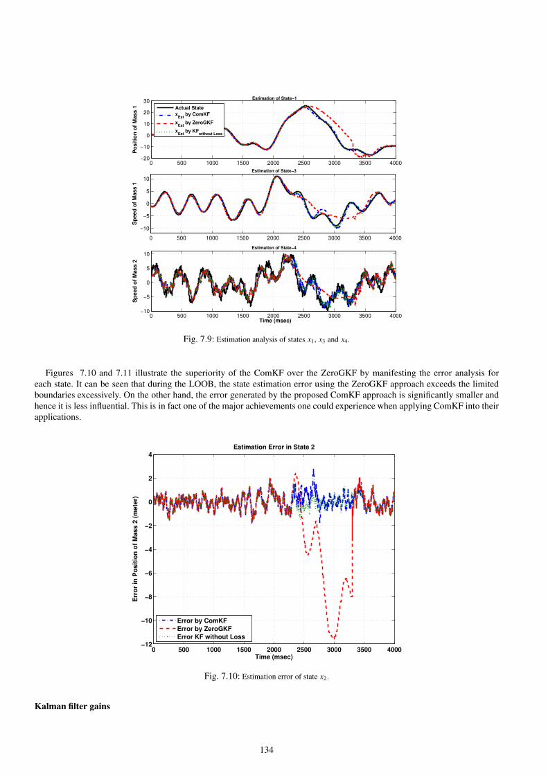
0 500 1000 1500 2000 2500 3000 3500 4000−20
−10
0
10
20
30
Po
sit
ion
of
Mass 1
Estimation of State−1
Actual State
xEst
by ComKF
xEst
by ZeroGKF
xEst
by KFwithout Loss
0 500 1000 1500 2000 2500 3000 3500 4000
−10
−5
0
5
10
Sp
eed
of
Mass 1
Estimation of State−3
0 500 1000 1500 2000 2500 3000 3500 4000−10
−5
0
5
10
Time (msec)
Sp
eed
of
Mass 2
Estimation of State−4
Fig. 7.9: Estimation analysis of states x1, x3 and x4.
Figures 7.10 and 7.11 illustrate the superiority of the ComKF over the ZeroGKF by manifesting the error analysis for
each state. It can be seen that during the LOOB, the state estimation error using the ZeroGKF approach exceeds the limited
boundaries excessively. On the other hand, the error generated by the proposed ComKF approach is significantly smaller and
hence it is less influential. This is in fact one of the major achievements one could experience when applying ComKF into their
applications.
0 500 1000 1500 2000 2500 3000 3500 4000−12
−10
−8
−6
−4
−2
0
2
4
Time (msec)
Err
or
in P
osit
ion
of
Mass 2
(m
ete
r)
Estimation Error in State 2
Error by ComKF
Error by ZeroGKF
Error KF without Loss
Fig. 7.10: Estimation error of state x2.
Kalman filter gains
134

0 500 1000 1500 2000 2500 3000 3500 4000−20
−10
0
10
Po
sit
ion
Err
or
(m)
Estimation Error in State 1
Error by ComKF
Error by ZeroGKF
Error by KFwithout Loss
0 500 1000 1500 2000 2500 3000 3500 4000
−5
0
5
Sp
ee
d E
rro
r (m
/se
c)
Estimation Error in State 3
0 500 1000 1500 2000 2500 3000 3500 4000−10
−5
0
5
10
Time (msec)
Sp
ee
d E
rro
r (m
/se
c)
Estimation Error in State 4
Fig. 7.11: Estimation error of states x1, x3 and x4.
The Kalman filter gains computed based on the ZeroGKF and ComKF approaches are shown in Figures 7.12 and 7.13,
respectively. As shown in Figure 7.12, Kalman filter gains reached their steady state values in the failure-free case (no LOOB)
in about 2 seconds. In the event of LOOB, the gains are forces to zero until LOOB is recovered with the zeroGKF approach. It
is also worthwhile to stress that at the time of switching from ZeroGKF back to the normal Kalman filter, there are undesirable,
excessive oscillations (also called the wind-up) in the gains to help hold the system’s state swiftly. Kalman filter gains using
ComKF are shown in Figure 7.13 and compared with that of the normal operation. Due to the gains being calculated online, it
can be seen that when the LOOB occurs, the compensated Kalman filter gains are very close to those of the original estimation
system. This indicates that the proposed filter, ComKF, could successfully predict the state estimation of the original systems
even if such a long period of loss of observation has occurred. Clearly, such an optimal compensated filter will generate
minimum errors for the estimated vector.
7.7 Summary
In this chapter two more nonlinear state estimation methods have been discussed, namely the unscented Kalman filters (UKF)
and the state dependent Riccati equation (SDRE) observer. Similar to earlier chapters, in addition to the introduction of al-
gorithms, application examples were given. More interestingly, usage and performances of various estimation methods were
compared and discussed. It is believed such arrangement would benefit readers in familiarising themselves with those nonlinear
estimation methods as well as in choosing more suitable methods for their applications.
The last part of the chapter discussed the robustness property of filtering approaches. The discussion is brief. Interested
readers may further consult relevant literatures. For example, another interesting case study on dealing with missing data can
be found in [65].
State estimation for nonlinear systems is an important component in control systems research and communication research
as well as in their applications. It is also an on-going research subject area. All the approaches discussed in this book are most
popular and useful in Authors’ opinion. However they are by no means exhaustive. For example, the particle filters [6, 42, 94]
and the sliding-mode observers [32, 34, 102] have been proposed and researched for the state estimation problems for nonlinear
control systems. Like in almost all engineering and scientific fields, there is no the “best” approach in nonlinear filtering. The
selection of filtering methods which turn out to be most effective and efficient depends on the understanding of the real world
problem at hand and on designer’s familiarisation of the filtering methods. That of course makes the life of researchers and
industrial engineers challenging and fun.
135
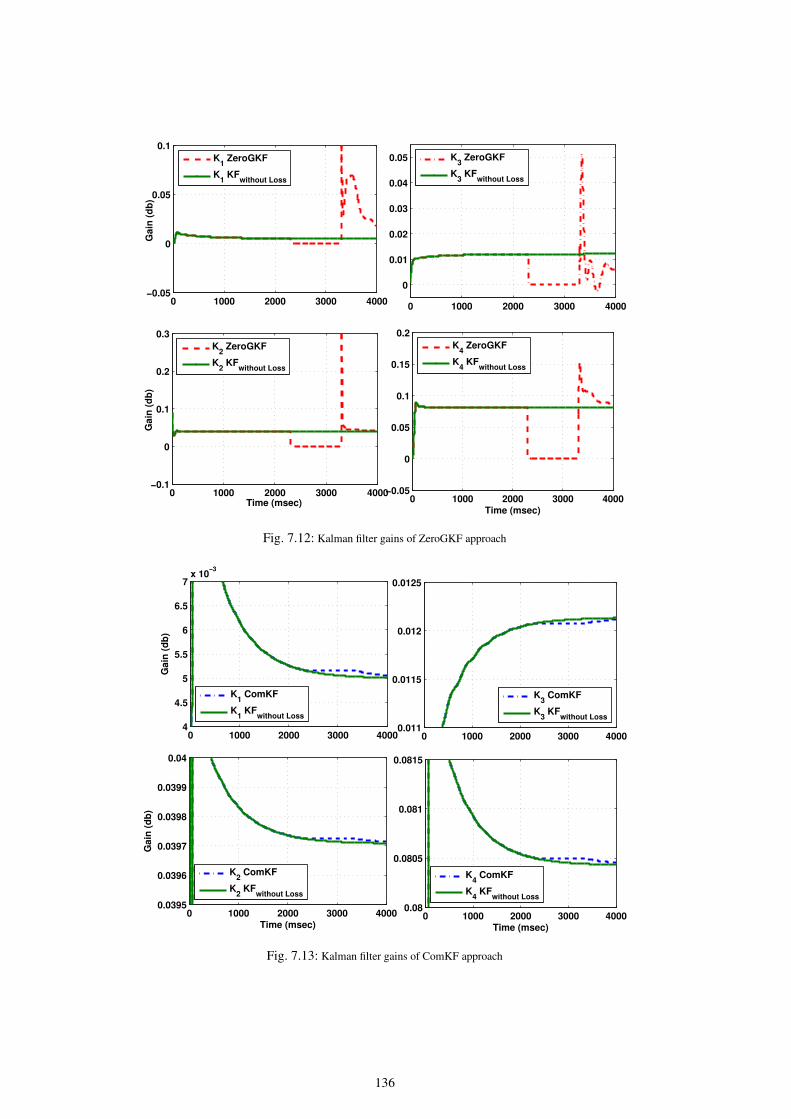
0 1000 2000 3000 4000−0.05
0
0.05
0.1
0.15
0.2
Time (msec)
K4 ZeroGKF
K4 KF
without Loss
0 1000 2000 3000 4000
0
0.01
0.02
0.03
0.04
0.05
K3 ZeroGKF
K3 KF
without Loss
0 1000 2000 3000 4000−0.1
0
0.1
0.2
0.3
Time (msec)
Ga
in (
db
)
K2 ZeroGKF
K2 KF
without Loss
0 1000 2000 3000 4000−0.05
0
0.05
0.1
G
ain
(d
b)
K1 ZeroGKF
K1 KF
without Loss
Fig. 7.12: Kalman filter gains of ZeroGKF approach
0 1000 2000 3000 40004
4.5
5
5.5
6
6.5
7x 10
−3
Gain
(d
b)
K1 ComKF
K1 KF
without Loss
0 1000 2000 3000 40000.08
0.0805
0.081
0.0815
Time (msec)
K4 ComKF
K4 KF
without Loss
0 1000 2000 3000 40000.0395
0.0396
0.0397
0.0398
0.0399
0.04
Time (msec)
Gain
(d
b)
K2 ComKF
K2 KF
without Loss
0 1000 2000 3000 40000.011
0.0115
0.012
0.0125
K3 ComKF
K3 KF
without Loss
Fig. 7.13: Kalman filter gains of ComKF approach
136

References
[1] DS1103 PPC Controller Board catlogue, Paderborn, Germany, 2008, howpublished= https://www.dspace.com/en/
inc/home/products/hw/singbord/ppcconbo.cfm, note = Accessed: 10 Feb 2018.
[2] MITSUBISHI Intelligent power modules catologue, 1998, howpublished= http://www.mitsubishielectric.com/
semiconductors/files/manuals/powermos6_0.pdf, note = Accessed: 10 Feb 2018.
[3] P. D. Allison. Missing data: Quantitative applications in the social sciences. British Journal of Mathematical and
Statistical Psychology, 55(1):193–196, 2002.
[4] B. D. O. Anderson and J. B. Moore. Optimal filtering. Englewood Cliffs, 21:22–95, 1979.
[5] I. Arasaratnam and S. Haykin. Cubature kalman filters. IEEE Transactions on automatic control, 54(6):1254–1269,
2009.
[6] M. S. Arulampalam, S. Maskell, N. Gordon, and T. Clapp. A tutorial on particle filters for online nonlinear/non-gaussian
bayesian tracking. IEEE Transactions on signal processing, 50(2):174–188, 2002.
[7] R. N. Banavar and J. L. Speyer. A linear-quadratic game approach to estimation and smoothing. In American Control
Conference, 1991, pages 2818–2822. IEEE, 1991.
[8] B. Bandyopadhyay, F. Deepak, and K.-S. Kim. Sliding mode control using novel sliding surfaces, volume 392. Springer,
2009.
[9] B. Bandyopadhyay and D. Fulwani. High-performance tracking controller for discrete plant using nonlinear sliding
surface. IEEE Transactions on Industrial Electronics, 56(9):3628–3637, 2009.
[10] H. Banks, B. Lewis, and H. Tran. Nonlinear feedback controllers and compensators: a state-dependent riccati equation
approach. Computational Optimization and Applications, 37(2):177–218, 2007.
[11] Y. Bar-Shalom, X. R. Li, and T. Kirubarajan. Estimation with applications to tracking and navigation: theory algorithms
and software. John Wiley & Sons, 2004.
[12] T. Basar. Optimum performance levels for minimax filters, predictors and smoothers. Systems & Control Letters,
16(5):309–317, 1991.
[13] G. Bierman, M. R. Belzer, J. S. Vandergraft, and D. W. Porter. Maximum likelihood estimation using square root
information filters. IEEE transactions on automatic control, 35(12):1293–1298, 1990.
[14] P. P. Biswas, R. Srivastava, S. Ray, and A. N. Samanta. Sliding mode control of quadruple tank process. Mechatronics,
19(4):548–561, 2009.
[15] R. Blind, S. Uhlich, B. Yang, and F. Allgower. Robustification and optimization of a kalman filter with measurement
loss using linear precoding. In American Control Conference, 2009. ACC’09., pages 2222–2227. IEEE, 2009.
[16] M. E. Campbell and W. W. Whitacre. Cooperative tracking using vision measurements on seascan uavs. IEEE Transac-
tions on Control Systems Technology, 15(4):613–626, 2007.
[17] N. A. Carlson. Federated square root filter for decentralized parallel processors. IEEE Transactions on Aerospace and
Electronic Systems, 26(3):517–525, 1990.
[18] K. B. Chandra, D.-W. Gu, and I. Postlethwaite. Square root cubature information filter. IEEE Sensors Journal, 13(2):750–
758, 2013.
[19] K. P. B. Chandra. Nonlinear State Estimation Algorithms and their Applications. PhD thesis, University of Leicester,
2013.
[20] K. P. B. Chandra, D.-W. Gu, and I. Postlethwaite. Square root cubature information filter. IEEE Sensors Journal,
13(2):750–758, 2013.
[21] K. P. B. Chandra, D.-W. Gu, and I. Postlethwaite. A cubature H∞ filter and its square-root version. International Journal
of Control, 87(4):764–776, 2014.
[22] K. P. B. Chandra, D.-W. Gu, and I. Postlethwaite. Cubature H∞ information filter and its extensions. European Journal
of Control, 29:17–32, 2016.
137

[23] C. Chatfield. The analysis of time series: an introduction. CRC press, 2016.
[24] G. Cheng and K. Peng. Robust composite nonlinear feedback control with application to a servo positioning system.
IEEE Transactions on Industrial Electronics, 54(2):1132–1140, 2007.
[25] W. C. Chu. Speech coding algorithms: foundation and evolution of standardized coders. John Wiley & Sons, 2004.
[26] K. L. Chung. A course in probability theory. Academic press, 2001.
[27] T. Cimen. State-dependent riccati equation (sdre) control: A survey. IFAC Proceedings Volumes, 41(2):3761–3775,
2008.
[28] J. R. Cloutier. State-dependent riccati equation techniques: an overview. In American Control Conference, volume 2,
pages 932–936, 1997.
[29] M. Csorba. Simultaneous localisation and map building. PhD thesis, University of Oxford, 1998.
[30] M. G. Dissanayake, P. Newman, S. Clark, H. F. Durrant-Whyte, and M. Csorba. A solution to the simultaneous localiza-
tion and map building (slam) problem. IEEE Transactions on robotics and automation, 17(3):229–241, 2001.
[31] A. Doucet, S. Godsill, and C. Andrieu. On sequential monte carlo sampling methods for bayesian filtering. Statistics
and computing, 10(3):197–208, 2000.
[32] S. V. Drakunov. Sliding-mode observers based on equivalent control method. In Decision and Control, 1992., Proceed-
ings of the 31st IEEE Conference on, pages 2368–2369. IEEE, 1992.
[33] H. Durrant-Whyte et al. Introduction to estimation and the kalman filter. Australian Centre for Field Robotics, 28(3):65–
94, 2001.
[34] C. Edwards, S. K. Spurgeon, and R. J. Patton. Sliding mode observers for fault detection and isolation. Automatica,
36(4):541–553, 2000.
[35] G. A. Einicke and L. B. White. Robust extended kalman filtering. IEEE Transactions on Signal Processing, 47(9):2596–
2599, 1999.
[36] R. M. Eustice, H. Singh, J. J. Leonard, and M. R. Walter. Visually mapping the rms titanic: Conservative covariance
estimates for slam information filters. The international journal of robotics research, 25(12):1223–1242, 2006.
[37] S. Fekri, M. Athans, and A. Pascoal. Robust multiple model adaptive control (rmmac): A case study. International
Journal of Adaptive Control and Signal Processing, 21(1):1–30, 2007.
[38] M. Grewal and A. Andrews. Kalman filtering: theory and practice using matlab, 2001.
[39] M. Grewal and A. Andrews. Kalman filtering: theory and practice using matlab, 2001.
[40] M. S. Grewal and A. P. Andrews. Applications of kalman filtering in aerospace 1960 to the present [historical perspec-
tives]. IEEE Control Systems magazine, 30(3):69–78, 2010.
[41] M. J. Grimble and A. El Sayed. Solution of the h∞ optimal linear filtering problem for discrete-time systems. IEEE
Transactions on Acoustics, Speech, and Signal Processing, 38(7):1092–1104, 1990.
[42] G. Grisetti, C. Stachniss, and W. Burgard. Improved techniques for grid mapping with rao-blackwellized particle filters.
IEEE transactions on Robotics, 23(1):34–46, 2007.
[43] D.-W. Gu, P. H. Petkov, and M. M. Konstantinov. Robust control design with MATLAB R©. Springer Science & Business
Media, 2014.
[44] B. Hassibi, T. Kailath, and A. H. Sayed. Array algorithms for h/sup/spl infin//estimation. IEEE Transactions on Auto-
matic Control, 45(4):702–706, 2000.
[45] M. H. Hayes. Statistical digital signal processing and modeling. John Wiley & Sons, 2009.
[46] S. Huang, Z. Wang, and G. Dissanayake. Exact state and covariance sub-matrix recovery for submap based sparse eif
slam algorithm. In Robotics and Automation, 2008. ICRA 2008. IEEE International Conference on, pages 1868–1873.
IEEE, 2008.
[47] S. A. Imtiaz, K. Roy, B. Huang, S. L. Shah, and P. Jampana. Estimation of states of nonlinear systems using a particle
filter. In Industrial Technology, 2006. ICIT 2006. IEEE International Conference on, pages 2432–2437. IEEE, 2006.
[48] J. Ishihara, B. Macchiavello, and M. Terra. H8 estimation and array algorithms for discrete-time descriptor systems. In
Decision and Control, 2006 45th IEEE Conference on, pages 4740–4745. IEEE, 2006.
[49] K. Ito and K. Xiong. Gaussian filters for nonlinear filtering problems. IEEE transactions on automatic control,
45(5):910–927, 2000.
[50] C. Jaganath, A. Ridley, and D. Bernstein. A sdre-based asymptotic observer for nonlinear discrete-time systems. In
Proceedings of the American Control Conference, 2005, pages 3630–3635, 2005.
[51] K. H. Johansson. The quadruple-tank process: A multivariable laboratory process with an adjustable zero. IEEE Trans-
actions on control systems technology, 8(3):456–465, 2000.
[52] J. K. Johnsen and F. Allower. Interconnection and damping assignment passivity-based control of a four-tank system. In
Lagrangian and Hamiltonian Methods for Nonlinear Control 2006, pages 111–122. Springer, 2007.
[53] S. Julier, J. Uhlmann, and H. F. Durrant-Whyte. A new method for the nonlinear transformation of means and covariances
in filters and estimators. IEEE Transactions on automatic control, 45(3):477–482, 2000.
138
[54] S. J. Julier and J. K. Uhlmann. Unscented filtering and nonlinear estimation. Proceedings of the IEEE, 92(3):401–422,
2004.
[55] M. Kaess and F. Dellaert. Covariance recovery from a square root information matrix for data association. Robotics and
autonomous systems, 57(12):1198–1210, 2009.
[56] T. Kailath. An innovations approach to least-squares estimation–part i: Linear filtering in additive white noise. IEEE
transactions on automatic control, 13(6):646–655, 1968.
[57] T. Kailath, A. H. Sayed, and B. Hassibi. Linear estimation, volume 1. Prentice Hall Upper Saddle River, NJ, 2000.
[58] R. E. Kalman et al. A new approach to linear filtering and prediction problems. Journal of basic Engineering, 82(1):35–
45, 1960.
[59] P. Kaminski, A. Bryson, and S. Schmidt. Discrete square root filtering: A survey of current techniques. IEEE Transac-
tions on Automatic Control, 16(6):727–736, 1971.
[60] P. P. Kanjilal. Adaptive prediction and predictive control. Number 52. IET, 1995.
[61] H. K. Khalil. Noninear systems. Prentice-Hall, New Jersey, 2(5):5–1, 1996.
[62] N. Khan. Linear prediction approaches to compensation of missing measurements in kalman filtering. PhD thesis,
University of Leicester, 2012.
[63] N. Khan, S. Fekri, and D. Gu. Improvement on state estimation for discrete-time lti systems with measurement loss.
Measurement, 43(10):1609–1622, 2010.
[64] N. Khan and D.-W. Gu. Properties of a robust kalman filter. IFAC Proceedings Volumes, 42(19):465–470, 2009.
[65] N. Khan, M. I. Khattak, and D. Gu. Robust state estimation and its application to spacecraft control. Automatica,
48(12):3142–3150, 2012.
[66] T. Kim, H. Lee, and M. Ehsani. Position sensorless brushless dc motor/generator drives: review and future trends. IET
Electric Power Applications, 1(4):557–564, 2007.
[67] A. Kolmogorov. Interpolation and extrapolation of stationary random sequences.
[68] R. Krishnan. Permanent magnet synchronous and brushless DC motor drives. CRC press, 2017.
[69] M. J. Kurtz and M. A. Henson. Nonlinear output feedback control of chemical reactors. In American Control Conference,
Proceedings of the 1995, volume 4, pages 2667–2671. IEEE, 1995.
[70] Q. Lam, M. Xin, and J. Cloutier. Sdre control stability criteria and convergence issues: Where are we today addressing
practitioners’ concerns? In Infotech@ Aerospace 2012, page 2475. 2012.
[71] B.-K. Lee and M. Ehsani. Advanced simulation model for brushless dc motor drives. Electric power components and
systems, 31(9):841–868, 2003.
[72] D.-J. Lee. Nonlinear estimation and multiple sensor fusion using unscented information filtering. IEEE Signal Processing
Letters, 15:861–864, 2008.
[73] W. Li and Y. Jia. H-infinity filtering for a class of nonlinear discrete-time systems based on unscented transform. Signal
Processing, 90(12):3301–3307, 2010.
[74] Y.-W. Liang and L.-G. Lin. Analysis of sdc matrices for successfully implementing the sdre scheme. Automatica,
49(10):3120 – 3124, 2013.
[75] X. Liu and A. Goldsmith. Kalman filtering with partial observation losses. In Decision and Control, 2004. CDC. 43rd
IEEE Conference on, volume 4, pages 4180–4186. IEEE, 2004.
[76] M. Loeve. Probability theory, 3rd ed. New York, 1963.
[77] J. Makhoul. Linear prediction: A tutorial review. Proceedings of the IEEE, 63(4):561–580, 1975.
[78] L. A. McGee and S. F. Schmidt. Discovery of the kalman filter as a practical tool for aerospace and industry. 1985.
[79] S. Mehta and J. Chiasson. Nonlinear control of a series dc motor: theory and experiment. IEEE Transactions on industrial
electronics, 45(1):134–141, 1998.
[80] M. Mercangoz and F. J. Doyle. Distributed model predictive control of an experimental four-tank system. Journal of
Process Control, 17(3):297–308, 2007.
[81] M. Morf and T. Kailath. Square-root algorithms for least-squares estimation. IEEE Transactions on Automatic Control,
20(4):487–497, 1975.
[82] C. P. Mracek, J. Clontier, and C. A. D’Souza. A new technique for nonlinear estimation. In Control Applications, 1996.,
Proceedings of the 1996 IEEE International Conference on, pages 338–343. IEEE, 1996.
[83] A. G. Mutambara. Decentralized estimation and control for multisensor systems. CRC press, 1998.
[84] K. Napgal and P. Khargonekar. Filtering and smoothing in an h-infinity setting. IEEE Transactions on Automatic Control,
36:152–166, 1991.
[85] A. Nemra and N. Aouf. Robust ins/gps sensor fusion for uav localization using sdre nonlinear filtering. IEEE Sensors
Journal, 10(4):789–798, 2010.
[86] A. V. Okpanachi. Developing advanced control strategies for a 4-tank laboratory process. Master’s Thesis report, 2010.
[87] A. Papoulis and S. U. Pillai. Probability, random variables, and stochastic processes. Tata McGraw-Hill Education,
2002.
139
[88] P. Park and T. Kailath. New square-root algorithms for kalman filtering. IEEE Transactions on Automatic Control,
40(5):895–899, 1995.
[89] C. L. Phillips, J. M. Parr, and E. A. Riskin. Signals, systems, and transforms. Prentice Hall, 1995.
[90] D. Potnuru, K. P. B. Chandra, I. Arasaratnam, D.-W. Gu, K. A. Mary, and S. B. Ch. Derivative-free square-root cubature
kalman filter for non-linear brushless dc motors. IET Electric Power Applications, 10(5):419–429, 2016.
[91] M. L. Psiaki. Square-root information filtering and fixed-interval smoothing with singularities. Automatica, 35(7):1323–
1331, 1999.
[92] T. Raff, S. Huber, Z. K. Nagy, and F. Allgower. Nonlinear model predictive control of a four tank system: An experimental
stability study. In Control Applications, 2006. CCA’06. IEEE International Conference on, pages 237–242. IEEE, 2006.
[93] J. Raol and G. Girija. Sensor data fusion algorithms using square-root information filtering. IEE Proceedings-Radar,
Sonar and Navigation, 149(2):89–96, 2002.
[94] G. G. Rigatos. Particle filtering for state estimation in nonlinear industrial systems. IEEE transactions on Instrumentation
and measurement, 58(11):3885–3900, 2009.
[95] S. H. Said and F. M’Sahli. A set of observers design to a quadruple tank process. In Control Applications, 2008. CCA
2008. IEEE International Conference on, pages 954–959. IEEE, 2008.
[96] J. Sarmavuori and S. Sarkka. Fourier-hermite kalman filter. IEEE Transactions on Automatic Control, 57(6):1511–1515,
2012.
[97] L. Schenato. Optimal estimation in networked control systems subject to random delay and packet drop. IEEE transac-
tions on automatic control, 53(5):1311–1317, 2008.
[98] U. Shaked. h∞-minimum error state estimation of linear stationary processes. IEEE Transactions on Automatic Control,
35(5):554–558, 1990.
[99] J. S. Shamma and J. R. Cloutier. Existence of sdre stabilizing feedback. IEEE Transactions on Automatic Control,
48(3):513–517, 2003.
[100] X.-M. Shen and L. Deng. Game theory approach to discrete h∞ filter design. IEEE Transactions on Signal Processing,
45(4):1092–1095, 1997.
[101] L. Shi, M. Epstein, A. Tiwari, and R. M. Murray. Estimation with information loss: Asymptotic analysis and error
bounds. In Decision and Control, 2005 and 2005 European Control Conference. CDC-ECC’05. 44th IEEE Conference
on, pages 1215–1221. IEEE, 2005.
[102] Y. Shtessel, C. Edwards, L. Fridman, and A. Levant. Sliding mode control and observation, volume 10. Springer, 2014.
[103] G. Sibley, G. S. Sukhatme, and L. H. Matthies. The iterated sigma point kalman filter with applications to long range
stereo. In Robotics: Science and Systems, volume 8, pages 235–244, 2006.
[104] D. Simon. Optimal state estimation: Kalman, H infinity, and nonlinear approaches. John Wiley & Sons, 2006.
[105] B. Sinopoli, L. Schenato, M. Franceschetti, K. Poolla, M. I. Jordan, and S. S. Sastry. Kalman filtering with intermittent
observations. IEEE transactions on Automatic Control, 49(9):1453–1464, 2004.
[106] J.-J. E. Slotine, W. Li, et al. Applied nonlinear control, volume 199. Prentice hall Englewood Cliffs, NJ, 1991.
[107] H. W. Sorenson. Least-squares estimation: from gauss to kalman. IEEE spectrum, 7(7):63–68, 1970.
[108] M. H. Terra, J. Y. Ishihara, and G. Jesus. Fast array algorithms for h∞ information estimation of rectangular discrete-
time descriptor systems. In Control Applications,(CCA) & Intelligent Control,(ISIC), 2009 IEEE, pages 637–642. IEEE,
2009.
[109] J. Tsyganova and M. Kulikova. State sensitivity evaluation within ud based array covariance filters. IEEE Transactions
on Automatic Control, 58(11):2944–2950, Nov 2013.
[110] A. Uppal, W. Ray, and A. Poore. On the dynamic behavior of continuous stirred tank reactors. Chemical Engineering
Science, 29(4):967–985, 1974.
[111] V. Utkin, J. Guldner, and J. Shi. Sliding mode control in electro-mechanical systems, volume 34. CRC press, 2009.
[112] R. Vadigepalli, E. P. Gatzke, and F. J. Doyle. Robust control of a multivariable experimental four-tank system. Industrial
& engineering chemistry research, 40(8):1916–1927, 2001.
[113] P. Vaidyanathan. The theory of linear prediction. Synthesis lectures on signal processing, 2(1):1–184, 2007.
[114] P. Vaidyanathan. The theory of linear prediction. Synthesis lectures on signal processing, 2(1):1–184, 2007.
[115] R. Van Der Merwe. Sigma-point kalman filters for probabilistic inference in dynamic state-space models. 2004.
[116] S. V. Vaseghi. Advanced digital signal processing and noise reduction. John Wiley & Sons, 2008.
[117] T. Vercauteren and X. Wang. Decentralized sigma-point information filters for target tracking in collaborative sensor
networks. IEEE Transactions on Signal Processing, 53(8):2997–3009, 2005.
[118] M. Verhaegen and P. Van Dooren. Numerical aspects of different kalman filter implementations. IEEE Transactions on
Automatic Control, 31(10):907–917, 1986.
[119] M. R. Walter, R. M. Eustice, and J. J. Leonard. Exactly sparse extended information filters for feature-based slam. The
International Journal of Robotics Research, 26(4):335–359, 2007.
140

[120] N. Wiener. Extrapolation, interpolation, and smoothing of stationary time series, volume 7. MIT press Cambridge, MA,
1949.
[121] Y. Xiong and M. Saif. Sliding mode observer for nonlinear uncertain systems. IEEE transactions on automatic control,
46(12):2012–2017, 2001.
[122] I. Yaesh and U. Shaked. Game theory approach to optimal linear state estimation and its relation to the minimum h∞norm estimation. IEEE Transactions on Automatic Control, 37(6):828–831, 1992.
[123] F. Yang, Z. Wang, S. Lauria, and X. Liu. Mobile robot localization using robust extended h8 filtering. Proceedings of
the Institution of Mechanical Engineers, Part I: Journal of Systems and Control Engineering, 223(8):1067–1080, 2009.
141


Index
H∞ filter, 24
Autocorrelation, 10
Brushless DC motor, 58
Closed-loop system, 3
closed-loop system, 3
Continuous stirred tank reactor (CSTR), 108
Continuous-time system, 2
Control plant, 1
Control process, 1
Control system, 1
Convergence, 12
Correlation, 9
Covariance, 9
Cubature H∞ filter, 77
Cubature H∞ information filter, 80
Cubature information filter, 71
Cubature Kalman filter, 5, 53
Cubature transformation, 57
DC motor, 15, 45
Discrete-time system, 2
Discrete-time system model, 19, 24
Discrete-time system model-information filters, 69
Extended H∞ filter, 41, 43
Extended H∞ information filter, 76
Extended information filter, 42, 70
Extended Kalman filter, 4, 41
Extended Kalman information filter, 41
Feedback system, 3
Filtering, 7
Filters, 7
Gaussian distribution, 10
Information filter, 4, 22, 69
Input, 1
Kalman filter, 4, 19
Least square estimator, 13
Linear system, 2, 13
Luenberger state observer, 14
Mean, 8
Mean square error, 12
MIMO system, 1
Multivariable system, 1
Noise, 2
Nonlinear system, 2, 13
Normal distribution, 10
Open-loop system, 3
Output, 1
Parameter estimation, 13
Permanent magnet synchronous motor (PMSM), 96
Prediction, 7
Quadruple-tank system, 26
Random process, 10, 11
Random variable, 8, 20
Robustness, 13
Sensitivity, 13
SISO system, 1
SLAM, 47
Smoothing, 7
Square root H∞ filter, 85
Square root cubature H∞ filter, 90
Square root cubature H∞ information filter, 93
Square root cubature information filter, 88
Square root extended information filter, 85
Square root extended Kalman filter, 83
Square-root filter, 4
Stability, 12
Standard deviation, 9
State dependent coefficient (SDC), 117
State dependent Riccati equation (SDRE) observer, 117
State estimation, 1, 3, 7
Stationary process, 11
System model, 2, 13
System state, 1, 7
Time invariant system, 2
Unscented Kalman filter, 4
Unscented Kalman filter (UKF), 113, 115
Unscented transformation, 113
Variance, 9
White noise, 12
143