Analysis of Three Different Kalman Filter Implementations ... · Analysis of Three Different Kalman...

The Open Agriculture Journal, 2009, 3, 13-19 13

1874-3315/09 2009 Bentham Open

Open Access

Analysis of Three Different Kalman Filter Implementations for Agricultural Vehicle Positioning

M. Rodríguez1 and J. Gómez

*,2

1Lear Corporation, Valls, Tarragona, Spain

2Departamento de Teoría de la Señal, Comunicaciones e Ingeniería Telemática, Universidad de Valladolid, 47011 Va-

lladolid, Spain

Abstract: Conventional positioning techniques based on GPS receivers are not accurate enough to be used with autono-

mous guidance systems. High accuracy GPS receivers can be employed, but the cost of the system would be very high.

The alternative solution presented in this article is to combine the data provided by different positioning sensors using a

Kalman filter. The described procedure also uses an odometric estimation of the mobile position, based on the kinematic

model of the agricultural vehicle. Three different implementations of the Kalman filter are described, using different sen-

sor combinations but based on the same vehicle model.

Keywords: Automatic guidance, GPS, INS, Kalman filter, Sensor fusion.

INTRODUCTION

Autonomous vehicle guidance includes positioning tech-niques to determine vehicle position and speed, and control techniques which implement the required actions to move the vehicle through the desired trajectory. This article fo-cuses only on positioning techniques.

Positioning systems may be classified into absolute posi-tioning systems and relative positioning systems. The first group can be used to obtain the mobile position with respect to a global reference; on the other hand, the second group provides the mobile position with respect to its previous po-sition [1]. Nowadays, the most widely used positioning sys-tem for agricultural vehicles is the GPS system. However, there are many other different positioning techniques. Hague et al. describe several non GPS based positioning systems [2].

Each positioning system has advantages and disadvan-tages, and is more suitable for certain kind of applications. However, the best option is usually the fusion of data pro-vided by different positioning sensors. This increases the accuracy of the system and it is useful to avoid positioning problems, for example, if the GPS reception fails [3-7].

One of the most widely used methods for this fusion is the Kalman filter [8]. The Kalman filter combines measure-ment data with estimations, minimizing the mean square error of the predictions. Also, this filter can be used only with a GPS receiver, in order to improve accuracy as it is described in [9].

This paper shows the mathematical calculations related to the data fusion with Kalman filter, for three different

*Address correspondence to this author at the Departamento de Teoría de la

Señal, Comunicaciones e Ingeniería Telemática, Universidad de Valladolid,

47011 Valladolid, Spain; Tel: (+34) 983423660; E-mail: [email protected]

configurations of the system. All the configurations use a GPS receiver and the same kinematic model (more complex kinematic models can be found in [10,11]). The first con-figuration combines the data from the GPS with a measure-ment of the steering angle. The second configuration uses an electronic compass instead of the steering angle sensor. Fi-nally the last configuration uses an IMU (Inertial Measure-ment Unit) and a steering angle sensor. Note that the most complex and expensive configuration is the last one, because it uses more sensors and calculation requirements are higher.

Kalman filtering is a powerful tool that has many other applications in agriculture, not only sensor fusion. For ex-ample, it can be used in topographic mapping or in obstacle detection algorithms [12, 13], but that is out of the scope of this article.

TRICYCLE MODEL

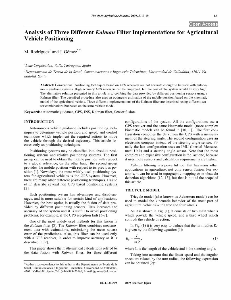
Tricycle model (also known as Ackerman model) can be used to model the kinematic behavior of the most part of agricultural vehicles with three and four wheels.

As it is shown in Fig. (1), it consists of two main wheels which provide the vehicle speed, and a third wheel which controls the vehicle direction.

In Fig. (1) it is very easy to deduce that the turn radius RC is given by the following equation (1):

RC =L

tg, (1)

where L is the length of the vehicle and the steering angle.

Taking into account that the linear speed and the angular speed are related by the turn radius, the following expression can be obtained (2):

14 The Open Agriculture Journal, 2009, Volume 3 Rodríguez and Gómez

= =v

RC=v tg

L, (2)

where is the angular speed of the mobile, is the orienta-tion of the vehicle in an external inertial reference system, and v is the longitudinal speed of the mobile. Usually v and are the control variables of the system, L is a known parame-ter, and the other variables must be estimated or measured. The proposed equations have many simplifications, more complex models can be found in the literature, see [4, 5], but the proposed model is enough for the purposes of this study.

KALMAN FILTER IN AN AGRICULTURAL VEHI-

CLE

Comparing the GPS with dead reckoning positioning signals, the GPS usually gives low frequency information position, and dead reckoning provides high frequency infor-mation position. The GPS positioning signal is often noisy but bounded, while the dead reckoning signal is often smooth but unbounded. All the facts indicate that GPS posi-tioning and dead reckoning positioning are complementary in nature, so that dead reckoning signals can be used to smooth out the short-term GPS error, and GPS signal can be used to recalibrate or align the dead reckoning drifting over a long period of time.

GPS signals arrive at fixed intervals, typically 1 second, and 0.2 seconds in the case of some more expensive models. Steering information from a steering sensor or from an elec-tronic compass is virtually continuous, so an odometry model can be run at a much greater repetition rate. When a

GPS reading arrives, it can be compared against the com-puted odometry estimation to correct drift and slip. This is basically the function of the Kalman filter.

A Kalman filter can be used to integrate the observations from absolute positioning and relative positioning. A very “friendly” introduction to the general idea of the Kalman filter can be found in Chapter 1 of [14], while a more com-plete introductory discussion can be found in [8], which also contains an interesting historical review. More extensive references include [13, 15-17].

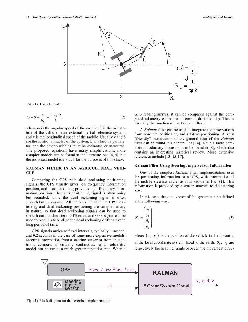
Kalman Filter Using Steering Angle Sensor Information

One of the simplest Kalman filter implementation uses the positioning information of a GPS, with information of the mobile steering angle, as it is shown in Fig. (2). This information is provided by a sensor attached to the steering axis.

In this case, the state vector of the system can be defined in the following way:

Xk =

xkyk

k

vk

, (3)

where xk , yk( ) is the position of the vehicle in the instant tk

in the local coordinate system, fixed to the earth. k , vk are

respectively the heading (angle between the movement direc-

Fig. (1). Tricycle model.

Fig. (2). Block diagram for the described implementation.

Analysis of Three Different Kalman Filter Implementations for Agricultural Vehicle Positioning The Open Agriculture Journal, 2009, Volume 3 15

tion of the vehicle and the north), and the vehicle speed at

time instant tk .

The system state equation can be expressed in the follow-ing way [11]:

Xk+1 = Fk Xk + k , (4)

where the state transition matrix (system matrix) Fk is de-

scribed as:

Fk =

1 0 0 T sen k

0 1 0 T cos k

0 0 1 Ttg

L0 0 0 1

. (5)

In equation (4) k is white noise, and T is the update

period of the Kalman filter. This means that the Kalman fil-

ter algorithm is executed each T seconds. The parameter

corresponds to the direction angle of the wheels.

The observations of the system are defined in the follow-ing way:

Zk =

xGPSyGPS

GPS

VGPS k

, (6)

where xGPS , yGPS , GPS and VGPS are the position, heading

and speed signals of the GPS respectively. Note that the up-

date rate of these measurements is very small, whereas the

update period of the filter is greater. The filter uses the

odometric estimations based on the system model to interpo-

late the intermediate system state values.

The observation equation can be written in the following way [11]:

Zk = Hk Xk + vk (7)

The matrix that defines the observation model is:

Hk =

1 0 0 0

0 1 0 0

0 0 1 0

0 0 0 1

(8)

It is the identity matrix because the measurements are

directly related with the system state variables. As in the

system state equation, here a white noise component vk is

introduced. Note that the system and observation white noise

variables vk and k are considered gaussian sequences of

zero mean and incorrelated. The initial value X0 of the sys-

tem state is a gaussian variable of known mean X0 , and co-

variance matrix P0 also known. This means that the follow-

ing conditions are met:

E k( ) = 0 , (9)

E vk( ) = 0 , (10)

E k iT( ) = k i( ) Qk , (11)

E vk viT( ) = k i( ) Rk , (12)

where n( ) =1, n = 0

0, n 0 is the Kronecker delta function,

Qk is the covariance matrix of the system noise, and Rk is

the covariance matrix of the observation noise. All of them

are defined and positive.

The adjustment of Qk and Rk is critical in the develop-

ment of the Kalman filter [11]. In this research, Rk is de-

fined in the following way:

Rk =

X(GPS)2 0 0 0

0 Y(GPS)2 0 0

0 0 (GPS)2 0

0 0 0 V(GPS)2

, (13)

where X(GPS)2

, Y(GPS)2

, (GPS)2

, V(GPS)2

are the covariances

of the GPS observations. Qk usually has the following shape:

Qk = q·

1 0 0 0

0 1 0 0

0 0 1 0

0 0 0 1

, (14)

where q is a parameter which measures the quality of the estimation. A small value means that the filter will give more importance to the estimation and less importance to the measurements. The value of this parameter must be chosen carefully, and there are several methods to determine the most convenient value for a specific application, see for ex-ample [8].

The equations for the estate estimation, update and gain matrix for this Kalman filter are listed in the following lines. See [11, 15, 16] for a more detailed explanation of these equations.

Extrapolation of the estimated estate:

X̂k = Fk 1 X̂k 1+

. (15)

Extrapolation of the error covariance:

Pk = Fk 1 Pk 1+ Fk 1

T+Qk 1 . (16)

Update of the estimated estate using the observations:

X̂k+= X̂k + Kk Zk Hk X̂k( ) . (17)

Update of the estimation error covariance:

Pk+= I Kk Hk( ) Pk . (18)

Gain matrix of the filter:

Kk = Pk HkT Hk Pk Hk

T+ Rk( )

1. (19)


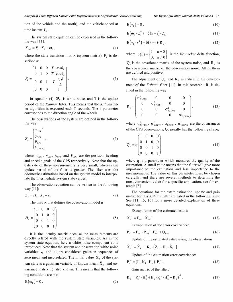
In the equations presented here, the (-) sign represents the a priori values of the covariance and the system state estima-tions, and the (+) sign represents the a posteriori values. Fig. (3) shows the sequence of operations for Kalman filtering, summarizing the previous equations.

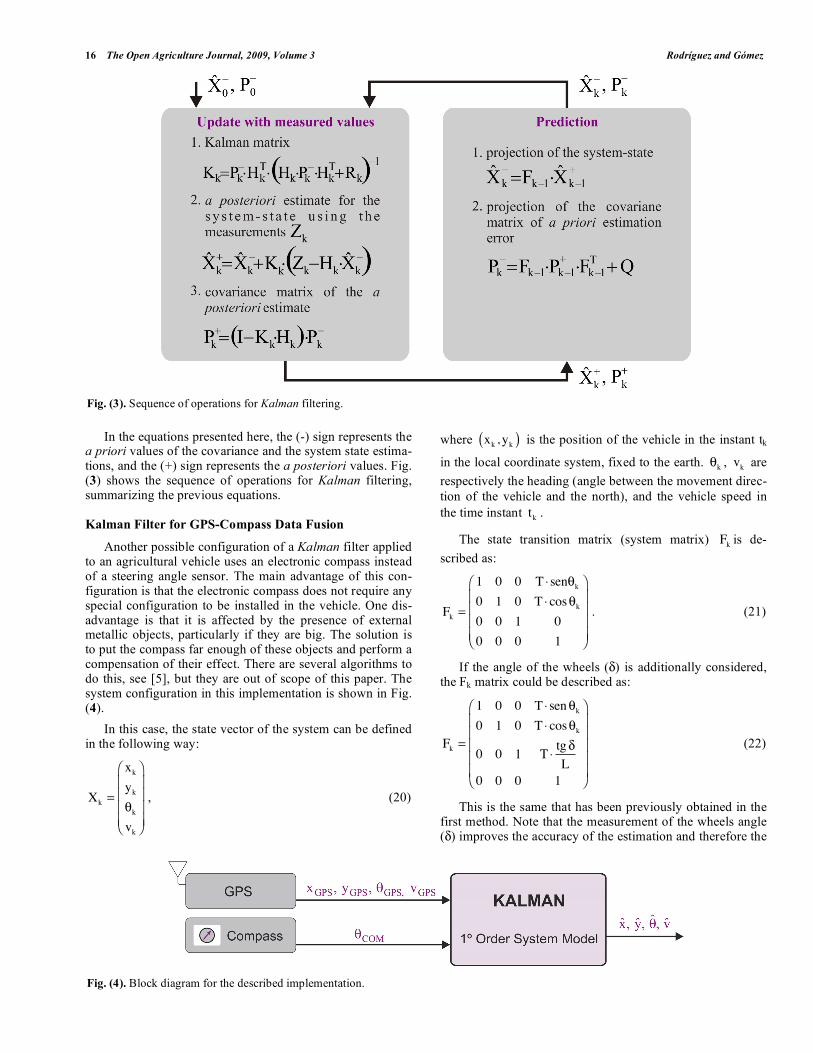
Kalman Filter for GPS-Compass Data Fusion

Another possible configuration of a Kalman filter applied to an agricultural vehicle uses an electronic compass instead of a steering angle sensor. The main advantage of this con-figuration is that the electronic compass does not require any special configuration to be installed in the vehicle. One dis-advantage is that it is affected by the presence of external metallic objects, particularly if they are big. The solution is to put the compass far enough of these objects and perform a compensation of their effect. There are several algorithms to do this, see [5], but they are out of scope of this paper. The system configuration in this implementation is shown in Fig. (4).


Xk =

xkyk

k

vk

, (20)

where xk , yk( ) is the position of the vehicle in the instant tk

in the local coordinate system, fixed to the earth. k , vk are

respectively the heading (angle between the movement direc-

tion of the vehicle and the north), and the vehicle speed in

the time instant tk .

The state transition matrix (system matrix) Fk is de-

scribed as:

Fk =

1 0 0 T sen k

0 1 0 T cos k

0 0 1 0

0 0 0 1

. (21)

If the angle of the wheels ( ) is additionally considered, the Fk matrix could be described as:

Fk =

1 0 0 T sen k

0 1 0 T cos k

0 0 1 Ttg

L0 0 0 1

(22)

This is the same that has been previously obtained in the first method. Note that the measurement of the wheels angle ( ) improves the accuracy of the estimation and therefore the

Fig. (3). Sequence of operations for Kalman filtering.



performance of the Kalman filter. However, it requires an additional sensor.


Zk =

xGPSyGPS

GPS

VGPS

COM k

, (23)


and speed signals of the GPS respectively, and COM is the

heading provided by the compass.


Hk =

1 0 0 0

0 1 0 0

0 0 1 0

0 0 0 1

0 0 1 0

. (24)

As in the first method, it is necessary to define the co-

variances of the different observations: X(GPS)2

, Y(GPS)2

,

(GPS)2

, V(GPS)2

, (COM)2

and the parameter q that defines the

quality of the estimation. The value of these parameters must

be chosen carefully. There are several methods to determine

the most convenient values for a specific application, see [8]

for more information.

The equations for the estate estimation, update and gain matrix for this Kalman filter are the same that for the first filter. See equations (15), (16), (17), (18) and (19).

Kalman Filter Using IMU Information

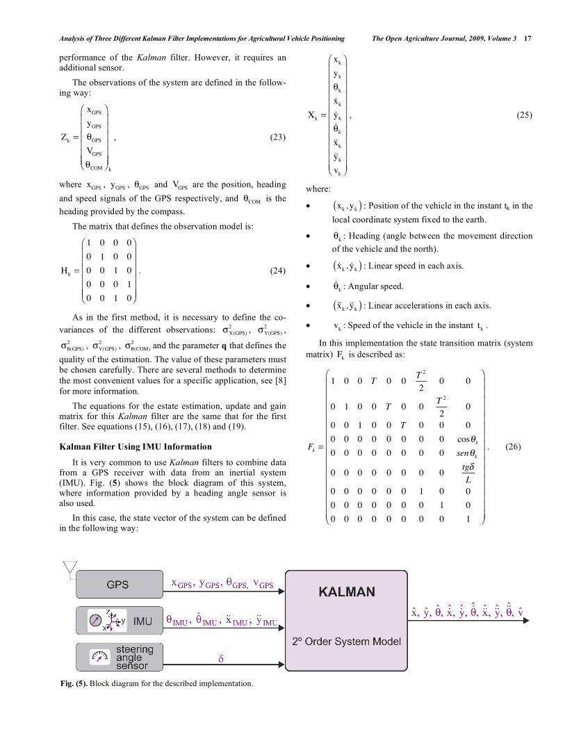
It is very common to use Kalman filters to combine data from a GPS receiver with data from an inertial system (IMU). Fig. (5) shows the block diagram of this system, where information provided by a heading angle sensor is also used.


Xk =

xkyk

k

xkyk

k

xkykvk

, (25)

where:

• xk , yk( ) : Position of the vehicle in the instant tk in the

local coordinate system fixed to the earth.

• k : Heading (angle between the movement direction

of the vehicle and the north).

• xk , yk( ) : Linear speed in each axis.

• k : Angular speed.

• xk , yk( ) : Linear accelerations in each axis.

• vk : Speed of the vehicle in the instant tk .

In this implementation the state transition matrix (system

matrix) Fk is described as:

Fk =

1 0 0 T 0 0T 2

20 0

0 1 0 0 T 0 0T 2

20

0 0 1 0 0 T 0 0 0

0 0 0 0 0 0 0 0 cos k

0 0 0 0 0 0 0 0 sen k

0 0 0 0 0 0 0 0tg

L0 0 0 0 0 0 1 0 0

0 0 0 0 0 0 0 1 0

0 0 0 0 0 0 0 0 1

. (26)



In the previous matrix T is the update period of the Kal-man filter and corresponds to the direction angle of the wheels. L is a parameter related to the tricycle model (length of the vehicle).


Zk =

xGPSyGPS

GPS

VGPS

IMU

IMU

xIMUyIMU k

, (27)


and speed signals of the GPS respectively.

IMU , IMU , xIMU , yIMU are respectively the heading, angular

speed and linear accelerations provided by the IMU.


Hk =

1 0 0 0 0 0 0 0 0

0 1 0 0 0 0 0 0 0

0 0 1 0 0 0 0 0 0

0 0 0 0 0 0 0 0 1

0 0 1 0 0 0 0 0 0

0 0 0 0 0 1 0 0 0

0 0 0 0 0 0 cos k sen k 0

0 0 0 0 0 0 sen k cos k 0

. (28)

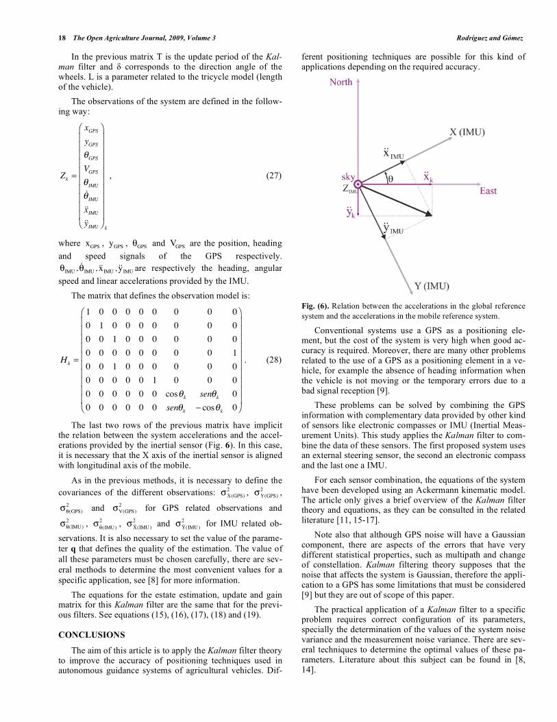
The last two rows of the previous matrix have implicit the relation between the system accelerations and the accel-erations provided by the inertial sensor (Fig. 6). In this case, it is necessary that the X axis of the inertial sensor is aligned with longitudinal axis of the mobile.

As in the previous methods, it is necessary to define the

covariances of the different observations: X(GPS)2

, Y(GPS)2

,

(GPS)2

and V(GPS)2

for GPS related observations and

(IMU)2

,

(IMU)2

,

X(IMU)2

and

Y(IMU)2

for IMU related ob-

servations. It is also necessary to set the value of the parame-

ter q that defines the quality of the estimation. The value of

all these parameters must be chosen carefully, there are sev-

eral methods to determine the most convenient values for a

specific application, see [8] for more information.

The equations for the estate estimation, update and gain matrix for this Kalman filter are the same that for the previ-ous filters. See equations (15), (16), (17), (18) and (19).

CONCLUSIONS

The aim of this article is to apply the Kalman filter theory to improve the accuracy of positioning techniques used in autonomous guidance systems of agricultural vehicles. Dif-

ferent positioning techniques are possible for this kind of applications depending on the required accuracy.

Fig. (6). Relation between the accelerations in the global reference

system and the accelerations in the mobile reference system.

Conventional systems use a GPS as a positioning ele-ment, but the cost of the system is very high when good ac-curacy is required. Moreover, there are many other problems related to the use of a GPS as a positioning element in a ve-hicle, for example the absence of heading information when the vehicle is not moving or the temporary errors due to a bad signal reception [9].

These problems can be solved by combining the GPS information with complementary data provided by other kind of sensors like electronic compasses or IMU (Inertial Meas-urement Units). This study applies the Kalman filter to com-bine the data of these sensors. The first proposed system uses an external steering sensor, the second an electronic compass and the last one a IMU.

For each sensor combination, the equations of the system have been developed using an Ackermann kinematic model. The article only gives a brief overview of the Kalman filter theory and equations, as they can be consulted in the related literature [11, 15-17].

Note also that although GPS noise will have a Gaussian component, there are aspects of the errors that have very different statistical properties, such as multipath and change of constellation. Kalman filtering theory supposes that the noise that affects the system is Gaussian, therefore the appli-cation to a GPS has some limitations that must be considered [9] but they are out of scope of this paper.

The practical application of a Kalman filter to a specific problem requires correct configuration of its parameters, specially the determination of the values of the system noise variance and the measurement noise variance. There are sev-eral techniques to determine the optimal values of these pa-rameters. Literature about this subject can be found in [8, 14].


REFERENCES

[1] Griepentrog HB, Blackmore BS, Vougioukas SG. In: Munack A,

Ed. CIGR Handbook of Agricultural Engineering Information Technology. Michigan USA 2006; Vol. VI: 195-220.

[2] Hague T, Marchant JA, Tillett ND. Ground based sensing systems for autonomous agricultural vehicles. Comp Electr Agric 2000; 25:

18-28. [3] Marchant JA, Hague T, Tillett DD. Row-following accuracy of an

autonomous vision-guided agricultural vehicle. Comp Electr Agric 1996; 16: 165-175.

[4] Guo LS, Zhang Q, Han S. Position Estimate of Off-Road Vehicles Using a Low Cost GPS and IMU. ASAE Paper No. 021157. Chi-

cago, Illinois, USA 2002. [5] Akira M, Noboru N, Kazunobu I. Automatic Navigation of Agri-

cultural Vehicle Using a Low Cost Attitude Sensor. ASAE Paper No. 701P1004. Kyoto, Japan 2004.

[6] Ehrl M, Stempfhuber WV, Demmel MR, Kainz M, Auernhammer H. AutoTrac – Accuracy of a RTK DGPS Based Autonomous Ve-

hicle Guidance System Under Field Conditions. ASAE Paper No. 701P1004. Kyoto, Japan 2004.

[7] Khot LR, Tang L, Blackmore SB, Norremark M. Navigational context recognition for an autonomous robot in a simulated tree

plantation. Trans ASAE 2006; 49(5): 1579-88.

[8] Sorenson HW. Least-Squares estimation: from Gauss to Kalman.

IEEE Spectrum 1970; 7: 63-8. [9] Han S, Zhang Q, Noh H. Kalman filtering of DGPS positions for a

parallel tracking application. Trans ASAE 2002; 45(3): 553-9. [10] Gelb A. Applied Optimal Estimation. MIT Press, Cambridge, MA

1974. [11] Grewal MS, Andrews AP. Kalman Filtering Theory and Practice.

Englewood Cliffs, New Jersey, Prentice-Hall, 1993. [12] Westphalen ML, Steward BL, Han S. Topographic mapping

through measurement of vehicle attitude and elevation. Trans ASAE 2004; 47(5): 1841-9.

[13] Kise M, Zhang Q, Noguchi N. An obstacle identification algorithm for a laser range finder-based obstacle detector. Trans ASAE 2005;

48(3): 1269-78. [14] Maybeck PS. Stochastic Models, Estimation, and Control, Aca-

demic Press, Inc. London, 1979; Vol. 1. [15] Lewis R. Optimal estimation with an introduction to stochastic

control theory, John Wiley & Sons, Inc. 1986. [16] Brown RG, Hwang PYC. Introduction to Random Signals and

Applied Kalman Filtering, 3rd ed. John Wiley & Sons, Inc. 1997. [17] Jacobs OLR. Introduction to Control Theory, 2nd ed. Oxford Uni-

versity Press, 1993.

Received: July 4, 2008 Revised: November 6, 2008 Accepted: December 17, 2008

© Rodríguez and Gómez; Licensee Bentham Open.

This is an open access article licensed under the terms of the Creative Commons Attribution Non-Commercial License (http: //creativecommons.org/licenses/by-

nc/3.0/) which permits unrestricted, non-commercial use, distribution and reproduction in any medium, provided the work is properly cited.

Analysis of Three Different Kalman Filter Implementations ... · Analysis of Three Different Kalman...

Documents

Transcript of Analysis of Three Different Kalman Filter Implementations ... · Analysis of Three Different Kalman...