Applied Mathematical Modelling xxx (2012) xxx–xxx

Contents lists available at SciVerse ScienceDirect

Applied Mathematical Modelling

journal homepage: www.elsevier .com/locate /apm

Numerical and laboratory prediction of smoke lofting in the atmosphereover large area fires

S.V. UtyuzhnikovSchool of Mechanical Aerospace and Civil Engineering, University of Manchester, Manchester M13 9PL, UK

a r t i c l e i n f o

Article history:Received 23 June 2011Received in revised form 12 February 2012Accepted 29 February 2012Available online xxxx

Keywords:Large-scale firePlumeCloudSmokeAtmosphereNuclear winter

0307-904X/$ - see front matter � 2012 Elsevier Inchttp://dx.doi.org/10.1016/j.apm.2012.02.050

E-mail address: s.utyuzhnikov@manchester.ac.uk

Please cite this article in press as: S.V. Utyuzharea fires, Appl. Math. Modell. (2012), http://d

a b s t r a c t

We analyze the lofting of aerosol in the atmosphere over a large scale fire. According to thewell-known theory of ‘‘nuclear winter’’, soot, rising in the atmosphere, may spread in thestratosphere and screen sun rays, which may in turn result in long-term catastrophic con-sequences for the climate. The height reached by the soot is critical for the climate model-ing because long-term global consequences can only be caused by a significant quantity ofsoot injected into the stratosphere. Most of the studies in the present literature are devotedto long-term modeling. The study of the initial (pyrocumulus) stage of the problem hasattracted much less attention with the amount of the soot injected into the mid-latitudestratosphere often being postulated. The amount of smoke that enters the stratosphereis crucial for climate consequences. It is therefore important to predict accurately the activestage of a large-scale fire, which is accompanied by the development of convective col-umns. The paper is devoted to the analysis of different approaches to the prediction ofthe altitude of smoke lofting over large scale fires. Some numerical, laboratory and analyt-ical methods are considered. The latter two approaches are based on the theory of similar-ity. The results obtained by different techniques are compared with each other. Specialattention is given to high resolution simulations, which accurately enough resolve gravitywaves.

� 2012 Elsevier Inc. All rights reserved.

1. Introduction

The theory of ‘‘nuclear winter’’ predicts long-lasting climate consequences of large-scale firestorms. According to thistheory, soot rises over the source of fire and is capable of penetrating into the middle and upper atmosphere [1]. Then,the smoke spreads in the stratosphere over the Earth and absorbs solar radiation for a long term. This inevitably leads tosignificant damages for the Earth climate.

First publications about the damage impact of large area fires on the climate appeared at the beginning of eighties inde-pendently by different groups (see [2,1,3]). Although different climate models were used, similar predictions were obtained:the climate consequences of a large area fire would cause a global climate disaster. As is concluded in [1], a significant drop ofthe average temperature would result in a ‘‘nuclear winter’’ and the climate changes would be severe. They might last abouta decade [4].

Those and further studies (see, e.g., recent publications: [4–6] have been based on global and regional climate modeling.There has been the detailed climate simulation of numerous scenarios. It has been shown that in the case of a nuclear explo-sion, the resulting fire inflicts more damage to the climate (via the lofting smoke) than the explosion itself. The plume, rising

. All rights reserved.

nikov, Numerical and laboratory prediction of smoke lofting in the atmosphere over largex.doi.org/10.1016/j.apm.2012.02.050

2 S.V. Utyuzhnikov / Applied Mathematical Modelling xxx (2012) xxx–xxx

over a fire, contains fire products such as black soot, smoke, ash and dust. Among the fire products, the soot is especiallycrucial for the climate consequences because it absorbs solar radiation.

It has been concluded that the plume of soot rises into the upper troposphere or lower stratosphere [4]. Moreover, addi-tional ascent to the upper stratosphere can be caused by solar induced lofting [5,7]. These effects are proved to be highlyimportant for the long-lasting climate consequences. Conversely, if aerosol is dispersed below the tropopause, its quantityrapidly diminishes due to rainfall as soon as its concentration drops to allow precipitation. As the result, the effect of fire onthe climate is local and holds for several months [6].

As noted above, the aerosol over a large scale fire can be lofted into the stratosphere due to heat convection and local aircirculation. Indeed, some smoke plumes have been observed after large forest fires [8–10]. According to the observation datareported in [11], the aerosol plume lofted to the lower stratosphere over the boreal forest fire in northwest Canada in 1998contained enough smoke to be visible. In recent numerical simulations of forest fires [12,13], it has been shown that if thefire diameter exceeds the atmospheric scale height, H0, estimated as 10 km, then deep penetration into the tropopause andlower stratosphere due to solar heating occurs.

Jost et al. [10] identify three major mechanisms which may be responsible for the aerosol injection into the mid-latitudestratosphere [10]: the overshooting of the original convection over the level of neutral buoyancy due to inertia and mixing atthe top, the effect of water vapor, and radiative heating followed by lofting of smoke. Overall, it seems that the driving forceof the troposphere-to-stratosphere transport is the extreme pyro-convection [11,14].

Much less study has been devoted to the stage of formation of convective columns over large-scale fires. However, thisstage is highly important for the prediction of the soot quantity to be injected into the stratosphere. As is noted in [9], theinjection of significant quantity of soot into the mid-latitude stratosphere is often postulated rather than accurately predicted.

In the literature, there are many publications devoted to the simulation of forest fires [8–10,15,12,13]. However, the typ-ical size of the fire in those studies is usually smaller than the height of the tropopause (atmospheric scale height H0). As isshown below, for such fires, the maximum height of the soot rise is well predicted by a self-similar solution. Overall, thereare only several publications in which large scale fires are addressed. We restrict our consideration by large scale fires be-cause only they can give the maximum estimate for the height of the soot rise [6]. By a large scale fire we mean a fire with atypical size to be comparable with the height of the tropopause (about 10 km).

Pioneering simulations of large-scale fires [16,17] were quite limited with respect to the typical physical size and numer-ical resolution. The flow over a fire was described by the compressible Reynolds Averaged Navier–Stokes equations (RANS).Penner et al. [16] simulated the Hamburg fire and predicted the maximum soot rise as high as 12 km and the altitude of neu-tral buoyancy as high as 8 km. These results were in rough agreement with limited available observations. In [16], relativelysmall areas of the fire (the radius less than 5 km) were considered. The information on the numerical algorithm was not pro-vided. Meanwhile, according to the pictures, the numerical resolution was quite low.

In [17], the physical time was limited by 1 h, while the fire radius was restricted by 10 km. The turbulent viscosity in theRANS equations was approximated by a piece-wise constant function that was, as shown by Muzafarov and Utyuzhnikov[18], a significant simplification. A first order scheme was used to obtain the numerical solution. Small and Heikes [17] rec-ognized that the area of the smoke was not adequately reproduced by the simulation. Thus, their prediction of the altitude ofplume rise (up to 19 km) did not seem very reliable. Meanwhile, Small and Heikes concluded that for large fires the height ofthe smoke injection mainly depended on the rate of energy release per unit area rather than the area of the fire.

Numerical modeling of an axis-symmetric fire source with the radius of 5 km was also carried out in [19]. Although theyused the turbulence model suggested in [16], the coefficient with the mixing length was different. As well as in [17], the firstorder scheme was exploited on a relatively rough mesh. The predicted maximum altitude of smoke injection was about14 km.

A detailed three-dimensional analysis of the Chisholm fire, which happened in Canada in 2001, was carried out byTrentmann et al. [13] using a sophisticated multiphase atmospheric model. The fire source was represented by a rectangulardomain of 15 km length and 0.5 km width. The length of the fire front was about 25 km. The maximum altitude of the pyro-convective columns reached 13 km.

The sensitivity analysis done by Luderer et al. [12] showed that heat release is the most significant factor affecting con-vection, while the fuel moisture is much less important. Overall, water vapor emitted from the fire does not significantlyaffect the evolution of the smoke plume [17,13]. According to Hiekes et al. [20], the moisture can lead to the redistributionof soot towards the upper level by a few kilometers.

As noted in [9], one of the key factors for this problem is related to intense gravity waves over a fire. For the first time, thegravity waves were resolved by Muzafarov and Utyuzhnikov [18] due to the use of compact approximations. In that paper, aswell as in [25], a wide range of fire areas was considered. It was demonstrated that the gravity waves essentially affect theformation of smoke columns.

In spite of the papers considered above, so far little has been done on comprehensive numerical simulation of large scalefires. As recently noted in [6], ‘‘Further numerical simulations of mass fires of a few kilometers radius would be useful tobetter understand the behavior of pyro-convection for fires of this scale’’. In that paper, it is recognized that there are stilluncertainties related to smoke plume heights.

It is to be noted that the problem is even more complicated due to luck of observation data and complete impossibility ofany full-scale experiment. Despite there are reliable estimates of plume height due to volcanic eruption in the literature (seee.g. [21–24]), these results cannot be applicable for large-scale fires as shown in the current paper.

Please cite this article in press as: S.V. Utyuzhnikov, Numerical and laboratory prediction of smoke lofting in the atmosphere over largearea fires, Appl. Math. Modell. (2012), http://dx.doi.org/10.1016/j.apm.2012.02.050

S.V. Utyuzhnikov / Applied Mathematical Modelling xxx (2012) xxx–xxx 3

In this paper, we consider computational, analytical and experimental predictions of the soot lofting in the atmosphereover a large scale fire. The paper is organized as follows.

In Section 2, the key computational results of papers by Muzafarov and Utyuzhnikov [18] and Konyukhou et al. [25] areanalyzed. Special attention is given to high resolution simulations of large-scale fires. These results are also considered indetail because they are not well-known in the western literature. It is shown that the average level of neutral buoyancyis approximately half the maximum plume rise altitude. Numerical simulations show that the aerosol cloud oscillates inthe atmosphere around its equilibrium level with the Brunt–Väisälä frequency. It is also obtained that, although there is aclear correlation between the area of a fire and the maximum height of the soot column, the maximum height is strictlybounded because the fire breaks into cells once the fire exceeds a radius of about 8 km.

The rest part of the paper is devoted to the analytical and experimental predictions of smoke lofting. Both approaches arebased on the theory of similarity. In the case of laboratory conditions, this theory is not applicable to the problem in questionstraightforward. However, it appears that, as demonstrated in the current paper, it can be used under some reasonableassumptions. In turn, the analytical solution can be obtained from the theory of similarity only for a so-called point sourcemodel described in Section 3. It appears to be accurate enough provided that the size of the fire can be neglected while thepower retaining. The laboratory modeling does not have such a limitation and can be carried out for a wide range of the inputparameters as shown in Section 4.

For the first time, all the three approaches mentioned above are compared with each other as described in Section 5. Inparticular, this allows us to define the limits of applicability for the point-source model. It is demonstrated that the self-sim-ilar analytical solution provides a quite good prediction for the altitude of smoke lofting until the radius of fire does notexceed 8 km. A reasonably good correspondence between the numerical results and laboratory re-scaled data occurs. Thisbrings an additional confirmation to the validity of the approximate similarity theory exploited in the experiments. It allowsus to design more comprehensive laboratory experiments which take it into account the effects of moisture and radiation.Overall, the considered results are not only relevant to the ‘‘nuclear winter’’ problem but also applicable to the analysis ofvery large wildfires such as the Red Lake 7 and Chisholm fires.

2. High resolution numerical simulation

Consider the mathematical formulation of the problem and key computational results obtained by Muzafarov andUtyuzhnikov [18] and Konyukhou et al. [25] via the use of compact Padé-type upwind approximations. These results arerequired for further comparison against analytical and laboratory predictions.

2.1. Statement of problem

The Reynolds-averaged Navier–Stokes equations for compressible gas flow are considered in the Cartesian coordinatesystem fyig ði ¼ 1;2;3Þ, where y3 is the coordinate in the direction normal to the Earth surface:

Pleasearea fi

@q@tþ @ei

inv@yiþ @lei

vis

@yi¼ �gf þ Q ;

where q is the vector of conserved variables, eiinv tensor of physical fluxes, f ;Q and svis source terms:

q ¼

qqV1

qV2

qV3

E

0BBBBBB@

1CCCCCCA; ei

inv ¼

qVi

qViV1 þ pdi1

qViV2 þ pdi2

qViV3 þ pdi3

ðEþ pÞVi

0BBBBBBB@

1CCCCCCCA; f ¼

000q

qV3

0BBBBBB@

1CCCCCCA; Q ¼

000

Q �

0BBB@

1CCCA;

eivis ¼

023@Vk

@yk di1 � ð@V1

@yi þ @Vi

@y1Þ23@Vk

@yk di2 � ð@V2

@yi þ @Vi

@y2Þ23@Vk

@yk di3 � ð@V3

@yi þ @Vi

@y3Þ23@Vk

@yk V i � ð@Vk

@yi þ @Vi

@ykÞVk � 1Pr

@h@yi

0BBBBBBBB@

1CCCCCCCCA:

Here, the summation over repeated indexes i; k ¼ 1;2;3 is assumed; dij is the Kronecker symbol; fV1;V2;V3g are the velocitycoordinates, q density, E ¼ qð�þ VkVk

2 Þ total energy, � internal energy, p pressure, h ¼ �þ p=q enthalpy, g free fall acceleration,l efficient coefficient of viscosity, Q � power of heat release per unit volume, Pr Prandtl number.

A dry atmosphere is considered in simulations. The parameters of the atmosphere correspond to the InternationalStandard Atmosphere [26].

cite this article in press as: S.V. Utyuzhnikov, Numerical and laboratory prediction of smoke lofting in the atmosphere over largeres, Appl. Math. Modell. (2012), http://dx.doi.org/10.1016/j.apm.2012.02.050

4 S.V. Utyuzhnikov / Applied Mathematical Modelling xxx (2012) xxx–xxx

The efficient coefficient of viscosity is described by the algebraic model used in [27,19] for modeling small- andlarge-scale fires in the atmosphere. As noted above, the model almost coincides with the model suggested in [28,16].The only difference is that the turbulent mixing length in the model by Gostintsev et al. [27] is shorter as much as1.6 times.

The fire source is modeled by a volume source similar to Hiekes et al. [20] and Gostintsev et al. [27,19]. It is consideredaxis-symmetric with the height, hs, equal to 100 m. In the computations, the fire radius varies between 5 km and 33 km. Theintensity of the volume source reaches its maximum value in 30 min. After 1 h the fire source is turned off to analyze howthis affects the height of the plume. Muzafarov and Utyuzhnikov [18] consider the case of a forest fire with Q � ¼ 0:5 kW=m3

that corresponds to the maximum energy release from the unit area of the surface equal to Qm ¼ 0:05 MW=m2 sinceQm ¼ Q �=hs. The aerosol is simulated by a ‘‘passive’’ contaminant permanently injected from the fire area. The passive con-taminant consists of transported weightless particles that do not affect the gas flow.

2.2. Numerical algorithm

In Muzafarov and Utyuzhnikov [18], a modified version of the upwind compact scheme developed by Tolstykh [29] isused. The original scheme has been modified to maintain the third order of accuracy for smooth solutions and in thesame time satisfy the entropy condition [30]. The scheme is strictly conservative, and has low dissipative and dispersiveerrors. The boundary conditions on the artificial open boundary are non-reflecting in the normal to the boundarydirection and no-friction in the tangential direction. The scheme allows one to obtain non-oscillatory solutions withoutthe use of any extra dissipative terms provided that the solution is sufficiently smooth [29]. The outlined propertiesof the third-order accurate upwind compact scheme are critical for long-term computations and resolution of gravitywaves.

The basic scheme for a hyperbolic set of one-dimensional equations can be formulated as follows.Consider the set of equations:

Pleasearea fi

@q@tþ @e@x¼ g; ð1Þ

where q 2 Rp is the vector of conserved quantities, e 2 Rp is the physical flux vector, g 2 Rp is the source term, p P 1.Since set (1) is hyperbolic, the Jacobian matrix E ¼ @e

@q can be decomposed into the product of three matrices E ¼ SKS�1,where S and K are square p� p matrices, S is the matrix with rows identical to the eigenvectors of the matrix E,K ¼ diagfk1; k2; . . . ; kpg is a diagonal matrix, ki; i ¼ 1; . . . ; p are the eigenvalues of matrix E.

Let us introduce a uniform spatial grid fxig; i ¼ 0;1; . . . ;N with the constant cell size h and a space of discrete functions fi,defined on this grid. Next, we consider basic operators:

A0fi ¼16

fi�1 þ23

fi þ16

fiþ1;

D0fi ¼ fiþ1 � fi�1;

D2fi ¼ fiþ1 � 2f i þ fi�1; i ¼ 1; . . . ;N � 1:

Then, the spatial discretisation of (1) is given by

Bx@q@t iþ Cxei ¼ Bxgi; ð2Þ

where Bx and Cx are the following finite-difference operators:

Bx ¼ A0 �14

MD0; Cx ¼1

2hðD0 �MD2Þ;

M ¼ diagfsignkig; i ¼ 0;1; . . . ;N:

The spatial discretisation scheme (2) is combined with a second order accurate temporal evolution method [31]. Overall, thescheme is proved to be high-resolution on smooth solutions. In particular, one can show via spectral analysis that, to resolvea harmonic wave, it is enough to have only five nodes per wave length [29].

In calculations, the spatial grid with refinement to the fire source was used. At least 10 nodes appeared in the fire sourcearea in the vertical direction, and 20 nodes, in horizontal coordinate direction. The adaptation in the physical domain wasreached via a transform of the coordinate system: n ¼ nðxÞ. Thus, in the computational domain, the grid remained uniform.On average, the space step was about 200 m. Thus, the chosen mesh was sufficient to resolve the internal gravity waves withthe wavelength of 2 km. In control accuracy computations, the number of nodes was doubled in each direction to make surethat the numerical resolution was accurate enough. In calculations, the Courant–Friedrichs–Lewy coefficient did not exceedthe value of 1. The artificial open boundary was placed far enough from the fire so that the solution was not sensitive to itslocation.

cite this article in press as: S.V. Utyuzhnikov, Numerical and laboratory prediction of smoke lofting in the atmosphere over largeres, Appl. Math. Modell. (2012), http://dx.doi.org/10.1016/j.apm.2012.02.050

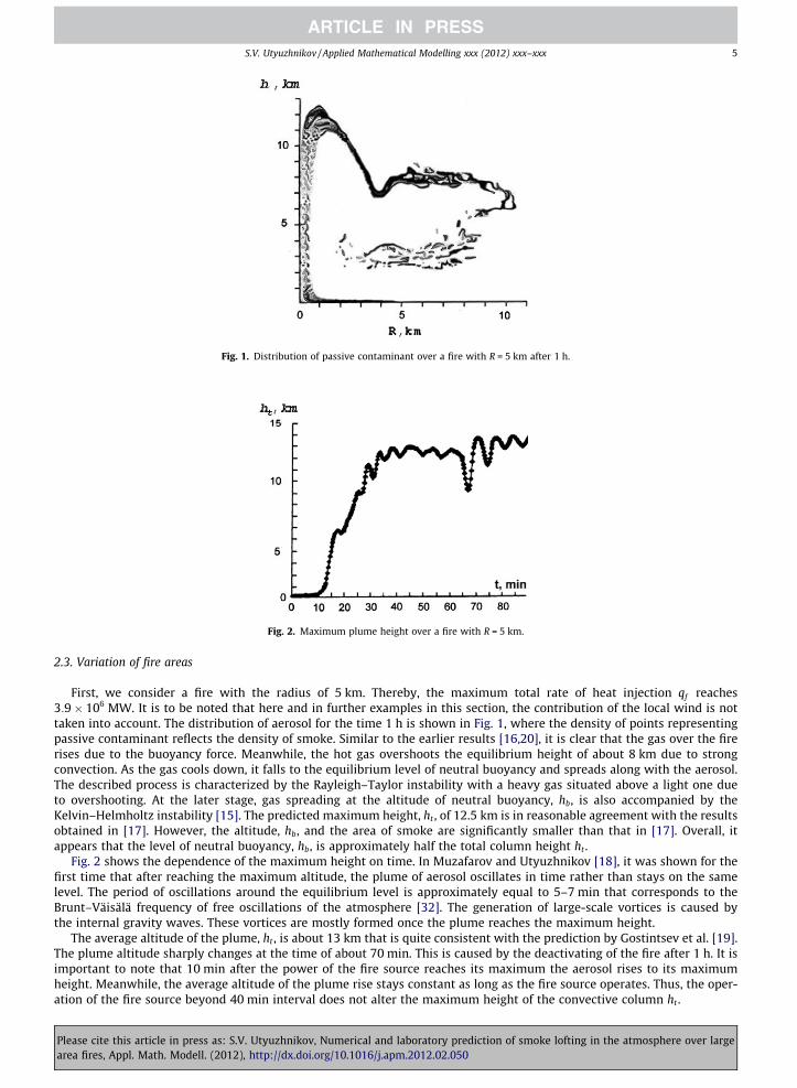
Fig. 1. Distribution of passive contaminant over a fire with R = 5 km after 1 h.

Fig. 2. Maximum plume height over a fire with R = 5 km.

S.V. Utyuzhnikov / Applied Mathematical Modelling xxx (2012) xxx–xxx 5

2.3. Variation of fire areas

First, we consider a fire with the radius of 5 km. Thereby, the maximum total rate of heat injection qf reaches3:9� 106 MW. It is to be noted that here and in further examples in this section, the contribution of the local wind is nottaken into account. The distribution of aerosol for the time 1 h is shown in Fig. 1, where the density of points representingpassive contaminant reflects the density of smoke. Similar to the earlier results [16,20], it is clear that the gas over the firerises due to the buoyancy force. Meanwhile, the hot gas overshoots the equilibrium height of about 8 km due to strongconvection. As the gas cools down, it falls to the equilibrium level of neutral buoyancy and spreads along with the aerosol.The described process is characterized by the Rayleigh–Taylor instability with a heavy gas situated above a light one dueto overshooting. At the later stage, gas spreading at the altitude of neutral buoyancy, hb, is also accompanied by theKelvin–Helmholtz instability [15]. The predicted maximum height, ht , of 12.5 km is in reasonable agreement with the resultsobtained in [17]. However, the altitude, hb, and the area of smoke are significantly smaller than that in [17]. Overall, itappears that the level of neutral buoyancy, hb, is approximately half the total column height ht .

Fig. 2 shows the dependence of the maximum height on time. In Muzafarov and Utyuzhnikov [18], it was shown for thefirst time that after reaching the maximum altitude, the plume of aerosol oscillates in time rather than stays on the samelevel. The period of oscillations around the equilibrium level is approximately equal to 5–7 min that corresponds to theBrunt–Väisälä frequency of free oscillations of the atmosphere [32]. The generation of large-scale vortices is caused bythe internal gravity waves. These vortices are mostly formed once the plume reaches the maximum height.

The average altitude of the plume, ht , is about 13 km that is quite consistent with the prediction by Gostintsev et al. [19].The plume altitude sharply changes at the time of about 70 min. This is caused by the deactivating of the fire after 1 h. It isimportant to note that 10 min after the power of the fire source reaches its maximum the aerosol rises to its maximumheight. Meanwhile, the average altitude of the plume rise stays constant as long as the fire source operates. Thus, the oper-ation of the fire source beyond 40 min interval does not alter the maximum height of the convective column ht .

Please cite this article in press as: S.V. Utyuzhnikov, Numerical and laboratory prediction of smoke lofting in the atmosphere over largearea fires, Appl. Math. Modell. (2012), http://dx.doi.org/10.1016/j.apm.2012.02.050

Fig. 3. Distribution of passive contaminant over a fire with R = 5 km after 1, 5 h.

Fig. 4. Maximum plume height over a fire with R = 11 km.

Fig. 5. Velocity field over a fire with R = 11 km at t = 90 min.

6 S.V. Utyuzhnikov / Applied Mathematical Modelling xxx (2012) xxx–xxx

Please cite this article in press as: S.V. Utyuzhnikov, Numerical and laboratory prediction of smoke lofting in the atmosphere over largearea fires, Appl. Math. Modell. (2012), http://dx.doi.org/10.1016/j.apm.2012.02.050

Fig. 6. Distribution of passive contaminant over a fire with R = 22 km after 80 min.

Fig. 7. Distribution of passive contaminant over a fire with R = 11 km after 20 min.

S.V. Utyuzhnikov / Applied Mathematical Modelling xxx (2012) xxx–xxx 7

The smoke distribution after 90 min is shown in Fig. 3. It can be seen that although the maximum altitude remains thesame as before, the concentration of the contaminant drops and the aerosol mostly spreads at the height of neutral buoy-ancy, hb, of about 7 km, which is situated in the tropopause.

One can expect that the increase of the radius of the fire, R, can lead to the increase of the maximum height of neutralbuoyancy. However, it appears that this is so only up to R � 11 km. After that the maximum altitude gradually decreasesand reaches the ultimate value below 15 km. For example, the change of the radius from 22 km to 33 km leads to a slightdrop of the maximum height from 16 km to 15 km.

Next, the dependence of the smoke plume height on time for the fire of R ¼ 11 km (qf ¼ 1:9� 107 MW) is shown in Fig. 4.One can see that after t ¼ 50 min, the average maximum altitude of plume rise is about 17 km and remains constant as longas the fire source continues to operate. The field of velocities over the fire at time 90 min is presented in Fig. 5. One can see aset vortices mostly generated in the atmosphere during the plume oscillations around the height of neutral buoyancy hb.

Finally, in Fig. 6, the distribution of aerosol over the fire with R = 22 km after 80 min is shown. One can see that the plumeheight, ht , is about 15 km, which is less than that of the fire of R ¼ 11 km. In turn, the computational results for the fire ofR ¼ 33 km confirmed the altitude ht is not much sensitive to the fire radius anymore.

The results discussed above suggest that if R is greater than 8 km, the fire breaks into local sources which tend to operateindependently. Eventually, the fire breaks up into coherent structures represented by the Benard cells. This is shown inFig. 7 which corresponds to the case of R ¼ 11 km after 20 min. The described effect was first obtained in Muzafarov andUtyuzhnikov [18].

Thus, one can see that the area of the fire is an important parameter with regards to the maximum altitude of the smokeplume. For large scale fires up to R � 11 km, it may well be a more important factor than the total heat release. Once the sizeof the fire exceeds R = 11 km, the maximum altitude of the smoke declines slightly, while the area of the smoke cloud even-tually increases. Overall, one can conclude that the fire area does not affect the maximum altitude of the smoke plume if thetypical size of the fire is significantly greater the atmospheric scale height H0. In this case, the fire source is broken up into aseries of local coherent structures operating independently.

In general, the predicted plume height is consistent with the altitude smoke injection of 13 km in the case of the Red Lake7 wildfire in Canada in 1986, provided by Lavoué [33]. The area of the fire was about 130 km2 that corresponds to the radiusof 7 km. It is interesting to note that approximately the same maximum altitude of the smoke plume is predicted by [13] forthe Chisholm fire, which had much less area of the fire: as less as one order of magnitude. However, in the case of theChisholm fire the typical fire size was 25 km. Thus, for the prediction of plume rise, the typical size of the fire source seemsa more crucial parameter than the total area of the fire.

In all computations the altitude of the neutral buoyancy, hb, is approximately half the total height of injection. This con-clusion approximately agrees with the results obtained in [12]: ht ¼ 11 km and hb ¼ 6 km. It is to be noted that in the case of

Please cite this article in press as: S.V. Utyuzhnikov, Numerical and laboratory prediction of smoke lofting in the atmosphere over largearea fires, Appl. Math. Modell. (2012), http://dx.doi.org/10.1016/j.apm.2012.02.050

Table 1Maximum plume height. Comparison against formula (3).

R; km ht ;A ¼ 0:255 ht ;A ¼ 0:31 ht;min ht;max

5 11.3 13.4 11.3 138 14.4 17.5 11.9 15

11 16.8 20.5 12.9 16.2

8 S.V. Utyuzhnikov / Applied Mathematical Modelling xxx (2012) xxx–xxx

a small-area source hb � 0:7ht as shown in [21]. Here, the small-area source means the typical size of the fire is much less theatmospheric scale height H0.

Our analysis demonstrates that the overshooting process of plume rise is followed by a significant fall of aerosol to theheight of neutral buoyancy hb. Meanwhile, some quantity of soot retains on the upper level due to the mixing mechanism.Thus, most aerosol appears in the tropopause. As noted before, the aerosol can eventually be heated by the sun and loftedinto the stratosphere. The simulation of such a process is beyond the scope of the current paper.

3. Self-similar analytical solution for a point source

If the area of the fire source can be neglected, then the maximum plume height can be predicted via the self-similar solu-tion for a point source [36]:

Pleasearea fi

zt ¼ Aq1=4f ; A ¼ constant; ð3Þ

where qf is the total rate of heat release in MW, zt is to be measured in km.It is interesting to compare the computational prediction for ht obtained by Muzafarov and Utyuzhnikov [18] against the

self-similar solution (3). There are at least two values for the constant A available in the literature: A ¼ 0:255 according to[34] and A ¼ 0:31 used in [27]. Table 1 gives the prediction of ht corresponding to the both values of constant A in formula (3)as well as the results of numerical simulation. It is accidental that these two constants provide good enough estimates for therange of ht in the oscillations around the level of neutral buoyancy: ht;min < ht < ht;max if R < 8 km.

It is easy to see that starting from R ¼ 11 km, the formula (3) is considerably violated. One can expect this because, assoon as the radius becomes comparable with the atmospheric scale height (about 10 km), H0, the physical problem is notself-similar anymore. In fact, since formula (3) is only obtained for a uniform atmosphere, it is not applicable even for a pointsource if the altitude of plume is high enough. As noted in [35], it should be modified with the account of variable stratifi-cation in the atmosphere above the tropopause.

For this purpose, introduce the parameter of stratification Ps as follows [36]:

Ps ¼ H0ddz

lnhatmðzÞhatmð0Þ

� �� �;

where hatm is the potential atmospheric temperature.Then, the modification suggested in [35] is given by

zt ¼ 1þ ðP0s =PsÞ3=8 � A

H0q1=4

f � 1� �� �

H0; ð4Þ

here P0s is the value of Ps in the tropopause. It is clear that if the altitude is not higher the tropopause, then formula (4) coin-

cides with the standard formula (3). The degree of 3/8 is chosen to fit available results for a point source in the case ofzt > H0.

The effect of modification (4) is shown in Fig. 8. The computational results by Muzafarov and Utyuzhnikov [18] corre-spond to the curves marked by triangles and diamonds. One can see that the modified self-similar solution (solid line) givesbetter prediction as the plume is above the tropopause. The comparison of analytical predictions (3) and (4) against someexperimental results is shown in the next section.

In the literature, there exists another analytical formula for the plume height, which is empirical in nature. Havinganalyzed many forest fires, Lavoué et al. [33] suggested a linear relationship between the frontal fire intensity and heightof the smoke injection. Meanwhile, from formula (3) it follows that the injection height of the smoke is proportionalto the square root of the radius: ht �

ffiffiffiRp

. Thus, for small enough fires (with the radius up to 5 km), the relationshipbetween the smoke height and frontal intensity is not linear provided that the frontal intensity is proportional to theperimeter of the fire. This conclusion is also confirmed by the observation data for forest fires given in [6]. Meanwhile,Trentmann et al. [13] and Luderer et al. [12] suggest that the linear relationship breaks down near the tropopause. Indeed,as noted above the smoke plume height reaches its maximum value at about R = 11 km and then decreases if the fireradius increases.

cite this article in press as: S.V. Utyuzhnikov, Numerical and laboratory prediction of smoke lofting in the atmosphere over largeres, Appl. Math. Modell. (2012), http://dx.doi.org/10.1016/j.apm.2012.02.050

Fig. 8. Total plume height vs radius of fire R;Qm ¼ 0:05 MW=m2. D and r correspond to computational results. Solid, dotted and dash-dotted linesrepresent analytical predictions for the energy-equivalent point source.

S.V. Utyuzhnikov / Applied Mathematical Modelling xxx (2012) xxx–xxx 9

4. Laboratory modeling

4.1. Approximate self-similarity

It appears that the problem is determined by 11 dimensional or 8 dimensionless parameters. Although the rigorous self-similarity cannot be obtained in the laboratory conditions, it can be reached for 6 key dimensionless parameters [36].

Following Morton et al. [36], to apply the theory of similarity, determine all independent key parameters. The flow essen-tially depends on 11 dimensional values such as the density qað0Þ, its gradient dq

dz, atmospheric pressure pað0Þ, the fire diam-eter D, the gravity acceleration g, kinematic viscosity m, the density of the injected gas qgð0Þ, the coordinates fr; zg ofcylindrical coordinate system, and the time t. Since there are only three independent dimensions, from the p-theorem itimmediately follows that the number of independent dimensionless parameters is equal to 8. The laboratory experimentswere carried out in a cylindrical chamber with a specific atmosphere [35,37], whereas the following key parametersretaining:

Pleasearea fi

P1 � Ps ¼ h0ddz

lnqcð0ÞqcðzÞ

� �� �; P2 ¼

qcð0Þqað0Þ

;

P3 �d0

h0¼ D

H0; P4 �

bzh0¼ z

H0;

P5 �brh0¼ r

H0; P6 �

btðgh0Þ

1=2 ¼t

ðgH0Þ1=2 ;

where qc is the density of air in the chamber; qg the density of air at the source; d0 the diameter of the ‘‘fire’’ source in thechamber; h0 the height of the ‘‘tropopause’’ in the chamber; br; bz;bt are the self-similar space and time variables, respectively.

The Grashof number Gr ¼ gD30=m was not exactly simulated. However, its value, calculated with respect to the turbulent

viscosity, was approximately retained. Finally, the Froude number Fr ¼ qað0Þgh0=pað0Þ was neglected in the experiments.From the theory of similarity it follows that all lengths in experimental results are to be scaled as much as D=d0 while the

time must be multiplied byffiffiffiffiffiffiffiffiffiffiffiD=d0

p.

It was supposed that H0 ¼ 11 km while h0 ¼ 20� 25 cm. The height h0 was determined as the altitude at whichqcðh0Þ ¼ 0:87qcð0Þ. Thus, in the experiments the typical size of the problem was reduced as much as 200 times.

4.2. Experimental setup

The experiments were carried out in a cylinder chamber 7 m in radius and 1.5 m in height. Freon mixed with air was in-jected from the bottom and top to the chamber and gradually taken away from the side. The gas injected through the bottomwas heavier the gas coming through the top as much as 5.9. The total rate of the injection, q, was 15 g/s. Thereby, a localstratified atmosphere was maintained in the experiments in such a way that

cite this article in press as: S.V. Utyuzhnikov, Numerical and laboratory prediction of smoke lofting in the atmosphere over largeres, Appl. Math. Modell. (2012), http://dx.doi.org/10.1016/j.apm.2012.02.050

Fig. 9.results,equival

10 S.V. Utyuzhnikov / Applied Mathematical Modelling xxx (2012) xxx–xxx

Pleasearea fi

qcðzÞqcð0Þ

¼ hatmð0ÞhatmðzÞ

:

The fire source was modeled by injected light gas with smoke. The velocity of injection w(0) satisfied the similarityconditions:

wð0Þ ¼Wð0Þ h0

H0

� �1=2

;

where W(0) is the typical velocity in the real conditions which was estimated as a function of the intensity of the fire sourceQm per unit area [36]:

Wð0Þ ¼ Q m

CpðT � TatmÞ;

where Cp is the heat capacity, T the temperature, Tatm ¼ 300 K. Thus, the equivalent total source power is equal to wð0Þpd2=4.

The injected gas was delivered through a grid to cause its turbulence. The radius of the source upon a scaling procedurevaried between 5 km and 22 km. The effects of moisture and radiation were not simulated in the experiments.

5. Comparison between laboratory, computational and analytical results

Test cases with d0=h0 < 1 showed a good correspondence between the experimental results and the point-source solution(4) with respect to the maximum height of a convective column ht .

There is a reasonably good correspondence between the experimental results [35] and computational results obtained in[25]. Two types of fire sources were considered distinguished by their intensity. The results are shown in Figs. 9 and 10respectively for Q m ¼ 0:073 MW=m2 and Q m ¼ 0:24 MW=m2. Such values of energy release rate represent wildfire and urbanfire [1]. The experimental results, marked by squares, were recalculated for real scales via multiplication of all space sizes byH0=h0 ¼ D=d0. The total plume height, ht , and altitude of neutral buoyancy, hb, are represented by the solid and dash-dottedlines, respectively. In turn, the appropriate computational results are marked by squares. The difference between the com-putational and laboratory results is mostly within 10%.

In Figs. 9 and 10, the crosses correspond to the point source with the equivalent power. As can be seen, the plume altitudeis significantly higher in this case. This result demonstrates that the point-source model is not applicable if R is greater 5 km.One can see that the modified analytical approximation given by formula (4) with A = 0.255 (dashed line) provides an accu-rate enough prediction for the energy-equivalent point source. In turn, the original formula (3) (dotted line) is basicallyapplicable only if ht does not exceed the tropopause height.

In [25] the algebraic turbulence model was similar to that used in Muzafarov and Utyuzhnikov [18] but one free param-eter of the model was modified. Breaking up the fire into multiple convective cells around R ¼ 11 km is observed in allregimes. As can be seen, the smoke column altitude significantly increases as the heat rate, Q m, increases.

Analyzing the results obtained in Muzafarov and Utyuzhnikov [18] and [25], one can conclude that the maximum height ofthe plume is proved to be quite sensitive to the turbulence model used. On the one hand, the model suggested by Gostintsev

Total plume height (solid line) and level of neutral buoyancy (dashed line) vs radius of fire R;Qm ¼ 0:073 MW=m2. r corresponds to computationalh, experimental results. Crosses, dashed and dotted lines represent experimental and analytical predictions (3) and (4), respectively, for the energy-ent point source.

cite this article in press as: S.V. Utyuzhnikov, Numerical and laboratory prediction of smoke lofting in the atmosphere over largeres, Appl. Math. Modell. (2012), http://dx.doi.org/10.1016/j.apm.2012.02.050

Fig. 10. Maximum plume height (solid line) and level of neutral buoyancy (dashed line) vs radius of fire R;Qm ¼ 0:24 MW=m2. r corresponds tocomputational results, h, experimental results. Crosses, dashed and dotted lines represent experimental and analytical predictions (3) and (4), respectively,for the energy-equivalent point source.

S.V. Utyuzhnikov / Applied Mathematical Modelling xxx (2012) xxx–xxx 11

et al. [27] provides a good correspondence with the self-similar solution for a point source (3) whereas the model by Penneret al. [16] gives a good enough prediction of the experimental data by Balabanov et al. [35]. On the other hand, there is adifference within a few kilometers between those two predictions.

Finally, in [38], 3D simulations were carried out for the fire with R = 10 km and the velocity of the wind 10 m/s. It ap-peared that the maximum height as well as the altitude and total area of the smoke cloud are not strongly affected bythe wind although the region of the smoke cloud is significantly displaced and deformed.

6. Summary

The prediction of smoke column height over a large-scale fire has been considered. Some computational, analytical andexperimental approaches have been analyzed and compared to each other. The self-similar analytical solution for a pointsource should be modified if the altitude of the smoke column reaches the tropopause. In turn, the point-source solutiongives good enough prediction only if the typical size of the fire is less the atmospheric scale height.

The laboratory modeling based on an approximate theory of similarity provides a reasonably good prediction for the evo-lution of smoke columns. According to laboratory and computational simulation, the aerosol over a large scale fire sequen-tially rises in the atmosphere, overshoots the equilibrium height, falls down and mostly spreads at some altitude. It appearsthat the altitude of neutral buoyancy is approximately half the maximum one. The plume oscillates in the atmospherearound some height of equilibrium with the frequency of natural atmospheric oscillations. The area of a fire can significantlyaffect the maximum height of the convective columns. In the case of large scale fires, the fire area may be more importantthan the intensity of heat release.

If the diameter of the fire exceeds twice the atmospheric scale height, then the fire breaks up into coherent structuresrepresented by the Benard cells. The deactivating of the energy source results in some drop of the maximum height. Ifthe typical size of the fire further increases, the height of the smoke column does not increase in contrast to the case ofan energy-equivalent point source. It appears that for very large-scale fires the total column height reaches some ultimatelevel above the tropopause.

In all considered possible cases, the altitude of neutral buoyancy remains below the stratosphere. Hence, most smokeappears in the tropopause and does not penetrate into the stratosphere. However, the long-term effect of the cross-tropo-pause transport of smoke can be reinforced by the self-lofting that leads to the subsequent injection of some quantity of aer-osol into the stratosphere. For the analysis of climate consequences, which is beyond the scope of the current paper, couplinga low-scale simulation of the initial (pyrocumulus) stage of the fire with global-scale climate models is required.

The effects of moisture, radiation and latent heat release should be taken into account in further experiments.

References

[1] R.P. Turco, O.B. Toon, T.P. Ackerman, J.B. Pollack, C. Sagan, Nuclear winter: global consequences of multiple nuclear explosions, Science 222 (1983)1283–1292.

[2] P.J. Crutzen, J.W. Birks, The atmosphere after a nuclear war: twilight at noon, J. Ambio. 11 (1982) 114–125. 2002.[3] V.V. Alexandrov, G.L. Stenchikov, On the modelling of the global consequences of the nuclear war, in: Proceeding in Applied Mathematics Computating

Centre, USSR Academy of Sciences, Moscow, 1983, p. 21.

Please cite this article in press as: S.V. Utyuzhnikov, Numerical and laboratory prediction of smoke lofting in the atmosphere over largearea fires, Appl. Math. Modell. (2012), http://dx.doi.org/10.1016/j.apm.2012.02.050

12 S.V. Utyuzhnikov / Applied Mathematical Modelling xxx (2012) xxx–xxx

[4] A. Robock, L. Oman, G.L. Stenchikov, Nuclear winter revisited with a modern climate model and current nuclear arsenals: still catastrophicconsequences, J. Geophys. Res. 112 (2007) D13107, http://dx.doi.org/10.1029/2006 JD008235.

[5] A. Robock, L. Oman, G.L. Stenchikov, O.B. Toon, C. Bardeen, R.P. Turco, Climate consequences of regional nuclear conflict, J. Atmosp. Chem. Phys. 7(2007) 2003–2012.

[6] O.B. Toon, R.P. Turco, A. Robock, C. Bardeen, L. Oman, G.L. Stenchikov, Atmospheric effects and societal consequences of regional scale nuclear conflictsand acts of individual nuclear terrorism, J. Atmosp. Chem. Phys. 7 (2007) 1973–2002.

[7] M.D. Fromm, O. Torres, D. Diner, D. Lindsey, B. Vant Hull, R. Servranckx, E.P. Shettle, Z. Li, Stratospheric impact of the Chisholm pyrocumulonimbuseruption: Part 1. Earth-viewing satellite perspective, J. Geophys. Res. 113 (D08202) (2008), http://dx.doi.org/10.1029/2007JD009153.

[8] M. Fromm, J. Alfred, K. Hoppel, R. Bevilacqua, E. Shettle, R. Servranckx, Z. Li, B. Stocks, Observations of boreal forest fire smoke in the stratosphere byPOAM III, SAGE II, and lidar in 1998, Geophys. Res. Lett. 27 (9) (2000) 1407–1410.

[9] M.D. Fromm, R. Servranckx, Transport of forest fire smoke above the tropopause by supercell convection, Geophys. Res. Lett. 30 (10) (2003) 1542,http://dx.doi.org/10.1029/2002GL016820.

[10] H.J. Jost, K. Drdla, A. Stohl, et al, In-situ observations of mid-altitude forest fire plumes deep in the stratosphere, Geophys. Res. Lett. 31 (2004) L11101,http://dx.doi.org/10.1020/2003GL019253.

[11] M.D. Fromm, R. Bevilacqua, R. Servranckx, J. Rosen, J.P. Thayer, J. Herman, D. Larko, Pyro-cumulonimbus, injection of smoke to the stratosphere:Observations and impact of superblowup in northwestern Canada on 3–4 August, 1998, Geophys. Res. Lett. 110 (2005) D08205, http://dx.doi.org/10.1029/2004JD005350.

[12] G. Luderer, J. Trentmann, T. Winterrath, C. Textor, M. Herzog, H.F. Graf, M.O. Andrea, Modeling of biomass smoke injection into the lower stratospherebe a large forest fire, Part II. Sensitivity studies, J. Atmosp. Chem. Phys. 6 (2006) 5261–5277.

[13] J. Trentmann, G. Luderer, T. Winterrath, M. Fromm, R. Servranckx, C. Textor, M. Herzog, M.O. Andrea, Modeling of biomass smoke injection into thelower stratosphere be a large forest fire, Part I. Reference study, J. Atmosp. Chem. Phys. 6 (2006) 5247–5260.

[14] M.D. Fromm, A. Tupper, D. Rosenfeld, R. Servranckx, R. McRae, Violent pyro-convective storm devastates Australia’s capital and pollutes thestratosphere, Geophys. Res. Lett. 33 (2006) L05815, http://dx.doi.org/10.1029/2005GL025161.

[15] P. Cunningham, S.L. Goodrick, M.Y. Hussaini, R.R. Linn, Coherent vortical structures in numerical simulations of buoyant plumes from wildland fires,Int. J. Wildland Fire 14 (2005) 61–75.

[16] J.E. Penner, L.C. Haselman Jr., L.L. Edwards, Smoke-plume distributions above large-scale fires: implications for simulations of nuclear winter, J. ClimateAppl. Meteorol. 25 (1986) 1434–1444.

[17] R.D. Small, K.E. Heikes, Early cloud formation by large area fires, J. Appl. Meteorol. 27 (1988) 654–663.[18] I.F. Muzafarov, S.V. Utyuzhnikov, Numerical modeling of convective columns above a large fire in the atmosphere, High Temp. 33 (4) (1995) 588–595.[19] Y.A. Gostintsev, N.P. Kopylov, A.M. Ryzhov, I.R. Khazanov, Numerical modeling of convective flows above large fires at various atmospheric conditions,

Combust. Explosions Shock Waves 27 (1991) 656–662.[20] K.E. Heikes, L.M. Ransohoff, R.D. Small, Numerical simulation of small area fires, Atmosp. Environ. 24 (A) (1990) 297–307.[21] C. Bonadonna, J. Phillips, Sedimentation from strong volanic plumes, J. Geophysical Research 108 (B7) (2003) 2340, http://dx.doi.org/10.1029/

2002JB002034.[22] Y. Ishimine, Sensitivity of the dynamics of volcanic eruption columns to their shape, Bull. Volcanol. 68 (2006) 516–537.[23] G. Carazzo, E. Kaminski, S. Tait, On the rise of tirbulent plumes: quantative effects of variable entrainment for submarine hydrothermal vents,

terrestrial and extra terrestrial explosive volcanism, J. Geophys. Res. 113 (2008), http://dx.doi.org/10.1029/2007JB005458.[24] E. Kaminski, A.-L. Chenet, C. Jaupart, V. Courtillot, Rise of volcanic plumes to the stratosphere aided by penetrative convection above large lava flows,

Earth Planet. Sci. Lett. 301 (2011) 171–178.[25] A.V. Konyukhov, M.V. Meshcheryakov, S.V. Utyuzhnikov, Numerical simulation of the processes of propagation of impurity from a large-scale source in

the atmosphere, J. High Temp. 37 (6) (1999) 873–879.[26] Standard Atmosphere, International Organization for Standardization, 1975.[27] Yu.A. Gostintsev, N.P. Kopylov, A.M. Ruzhov, I.R. Khasanov, Convective transport of combustion products in the atmosphere above large fires, J. Fluid

Dyn. 25 (4) (1990) 532–537.[28] J.E. Penner, L.C. Haselman, Smoke inputs to climate models: optical properties and height distribution, in: Proceedings of the International Seminar on

Nuclear War, Erice, E. Majorana Centre for Scientific, Culture, 1984, pp. 197–215.[29] A.I. Tolstykh, High Accuracy Non-centered Compact Difference Schemes for Fluid Dynamics Applications, World Scientific, Singapore, 1994.[30] I.F. Muzafarov, S.V. Utyuzhnikov, Application of compact finite-difference schemes to the initial boundary value problem for a hyperbolic system of

equations, J. Comput. Math. Math. Phys. 37 (3) (1997) 299–306.[31] R.M. Beam, R.F. Warming, An implicit factored scheme for comressible Navier–Stokes equations, AIAA J. 16 (4) (1978) 393–402.[32] E.E. Gossard, W.H. Hook, Waves in the Atmosphere, Elsevier, Amsterdam, 1975.[33] D. Lavoué, C. Liousse, H. Cachier, B.J. Stocks, J.D. Goldammer, Modeling of carbonaceous particles emitted by boreal and temperate wildfires at northen

latitudes, J. Geophys. Res. 105 (26) (2000) 871–890.[34] P.C. Manins, Cloud heights and stratospheric injections resulting from a thermonuclear war, Atmosp. Environ. 19 (8) (1985) 1245–1255.[35] V.A. Balabanov, M.A. Mechkov, A.T. Onufriev, N.A. Safarov, R.A. Safarov, V.E. Skorovarov, The dynamical pattern of the turbulent convective high-

altitude transport generated by large area sources of buoyancy in the stratified atmosphere, in: Proceedings of the 1st National Russian Conference onHeat Exchange, vol. 2, 1994, pp. 31–36 (in Russian).

[36] B.R. Morton, G.T. Taylor, Y.S. Turner, Turbulent gravitational convection from maintained and instantaneous sources, Proc. Royal Soc. A 234 (1956) 1–23.

[37] A.V. Konyukhov, M.V. Meshcheryakov, I.F. Muzafarov, A.T. Onufriev, N.A. Safarov, R.A. Safarov, S.V. Utyuzhnikov, Laboratory and numerical simulationof convective flow over large-scale source of energy, in: Co-ordination Meeting in INTAS/ERFORTAC Project an-European Network on Flow Turbulenceand Combustion Final Report, 1996.

[38] M.N. Antonenko, A.V. Konyukhov, L.M. Kraginskii, M.V. Meshcheryakov, S.V. Utyuzhnikov, Numerical modeling of intensive convective flow inatmosphere induced by large-scale fire, Int. J. Comput. Fluid Dyn. 11 (2) (2002) 128–132.

Please cite this article in press as: S.V. Utyuzhnikov, Numerical and laboratory prediction of smoke lofting in the atmosphere over largearea fires, Appl. Math. Modell. (2012), http://dx.doi.org/10.1016/j.apm.2012.02.050