KINEMATIC BEHAVIOR OF SOLID PARTICLES IN ENCLOSED LID-

DRIVEN CAVITY USING CIP METHOD

ALI AKBARI SHELDAREH

A project report submitted in partial fulfilment of the

Requirements for the award of the degree of

Master of Engineering (Mechanical Engineering)

Faculty of Mechanical Engineering

Universiti Teknologi Malaysia

FEBRUARY 2012

iii

To my beloved family and friends

And my respectful supervisor

Thank you for all kindness and sacrifices you made for me.

iv

ACKNOWLEDGEMENTS

In the name of Allah, the most Gracious, the Most Merciful.

I have faced difficulties during preparation of this thesis, but with the help

and support of Dr.Nor Azwadi Che Sidik, I have overcome all of them. I sincerely

thank Dr. Nor Azwadi Bin Che Sidik for his guidance, help and motivation. I have

learnt a lot from him and his positive contributions and responsibility were a boon to

me.

I would like to thank my Supervisor Dr. Nor Azwadi Bin Che Sidik, the Head

of Department of Postgraduate studies in the Mechanical Department for his warm

assistance in finalizing the research problem and giving useful comments. A great

deal of appreciation also goes to the Faculty of Mechanical Engineering (FKM). I am

especially grateful to my fellow course mate Arman Safdari, for his sincere

assistance, useful insights, and his positive contributions.

Nevertheless, I would like to thank to my family for loving me and being

supportive in the duration of completing this thesis. I wish to thank my parents,

Dr.Fereydoun Akbari Sheldareh and A. Ghanbari, for their love, support and

kindness. They have always been a source of inspiration and encouragement for me.

I wish to thank my brothers Arash and Amir Hossein who are always giving me

positive energy and kindness, brothers who are the apple of my eyes.

v

ABSTRACT

The Cubic Interpolated Pseudo-Particle Navier Stokes equation (CIP-NSE)

was applied to investigate the two-dimensional laminar square lid driven cavity flow

of water at Reynolds number 1000. CIP-NSE scheme was used to solve hyperbolic

term of the vorticity transport equation. In the CIP-NSE, the gradient and the value

of the vorticity at the nodes is determined and the stream function is then determined

using the vorticity equation. It is discovered that the numerical simulation of CIP-

NSE provided a very good agreement with the established benchmark results by

previous researchers. The Runge-Kutta method has been used to calculate the

velocity and position of the particle with the effects of Drag force and Gravitational

forces. The hard sphere model has been applied to show the collisions effect on

particles in the Lid-Driven cavity. The main result achieved from the investigation is

that, as the density of particles increases the number of particles collision in first

seconds of the investigation decreases and the number of particles settled on the floor

of the cavity increases, so for higher density of particles there have been large

number of particles settlement on the floor and the collision at starting of

investigation decrease as the particles moves slower, and for the lighter particles and

lower density of particles number of collision at starting of investigation in more as

the particles are lighter and move faster but the particles settlement on the floor of

cavity are less in compare to higher density of particles. All simulation have been

done for four different density of particle which are 1000, 1200, 1700, and 2000

(kg/m³).

vi

ABSTRAK

Persamaan Navier-Stokes untuk penentuan cubic pseudo-particle (CIP-NSE)

telah digunakan untuk mengkaji alirain air dalam rongga berpandukan penutup dua

matra dengan nombor Reynolds bersamaan dengan 1000. Kaedah CIP-NSE

digunakan untuk menyelesaikan istilah hiperbolik bagi persamaan perjalanan vortex.

Bagi CIP-NSE, kecerunan dan nilai vortex di nod ditentukan dan fungsi aliran

ditentukan oleh persamaan vortex. Keputusan daripada simulasi berangka CIP-NSE

didapati hampir serupa dengan keputusan daripada penyelidik sebelum ini. Kaedah

Runge-Kutta telah digunakan untuk meramal kelajuan dan kedudukan zarah dengan

mengamibil kira daya rintangan dan daya tarikan graviti. Model sfera keras telah

digunakan untuk menunjukkan kesan perlanggaran ke atas zarah di dalam rongga

berpandukan penutup. Kajian ini telah membuktikan bahawa semakin tinggi

ketumpatan zarah, kadar perlanggaran zarah di awal kajian semakin rendah.

Disebabkan ketumpatan yang tinggi, zarah-zarah akan tenggelam ke dasar rongga

tersebut, dan zarah tersebut bergerak dengan perlahan, seterusnya menyebabkan

kadar perlanggaran zarah yang rendah. Zarah yang ringan dan berketumpatan rendah

mempunyai kadar perlanggaran yang tinggi kerana zarah yang ringan bergerak

dengan lebih pantas dan seterusnya menghasilkan lebih banyak perlanggaran.

Kesemua simulasi telah dijalankan untuk empat nilai ketumpatan zarah iaitu 1000,

1200, 1700 dan 2000 (kg/m³).

vii

TABLE OF CONTENTS

CHAPTER TITLE PAGES

ACKNOWLEDGEMENTS iv

ABSTRACT v

ABSTRAK vi

LIST OF TABLES xi

LIST OF FIGURES xii

LIST OF ABBREVIATIONS xiv

LIST OF SYMBOLS xv

CHAPTER 1

INTRODUCTION 1

1.1 Introduction 1

1.2 Computational Fluid Dynamic (CFD) 4

1.2.1 Governing Equation in CFD 6

1.2.2 The Navier-Stokes Equations 7

1.3 Problem Statement 9

1.4 Objectives of the research 9

1.5 Significance of study 10

1.6 Scope of the Study 11

viii

CHAPTER 2

LITRITURE REVIEW 12

2.1 Introduction 12

2.2 Background of Study 13

2.2.1 The Navier-Stokes Equation 17

2.2.2 Analytical Solution to Navier-Stokes Application 18

2.3 Stream Function-Vorticity Navier-Stokes Approach 21

2.4 Essence of Finite Difference 22

2.5 Cubic Interpolated Pseudo-Particle (CIP) 23

2.6 Two-Phase Flows 24

2.7 Forces Acting on Particle 25

2.7.1 Gravitational Force 25

2.7.2 Buoyancy Force 26

2.7.3 Drag Force 26

2.8.1 Particle Collisions 27

2.8.2 Particle-Particle Collision 28

2.8.2.1 Hard Sphere Model 29

2.8.2.2 Soft Sphere Model 29

CHAPTER 3

RESEARCH METHODOLOGY 30

3.1 Introduction 30

3.2 Overview 31

3.3 Primary Data 31

3.3 Secondary Data 31

3.4 Governing Equations in Cavity Flow 32

3.5 Stream Function-Vorticity Approach 32

ix

3.5.1 Dimensionless Variables 35

3.5.2 Discretization 37

3.5.3 The Boundary Conditions 38

3.5.4 Grid Generation 42

3.6 One Dimensional Hyperbolic Equation With CIP 44

3.7 CIP-Navier Stokes Equation (CIP-NSE) 46

3.7.1 The Non-Advection Phase 48

3.7.2 The Advection Phase 53

3.8.1 The Flow of the Continuous Phase 58

3.8.2 The Flow of the Particle 59

3.9 Collision 62

3.9.1 Particle-Particle Collision 62

3.9.2 Particle-Wall Collision 67

3.10 Flow Chart 70

CHAPTER 4

RESULTS AND DISCUSSIONS 71

4.1 Introduction 71

4.2 Simulation of Fluid in Lid-Driven Cavity 72

4.3 Code Validation 73

4.3.1 Code Validation for Fluid 74

4.3.1.1 Code Validation of Fluid Flow Using CIP Method 79

4.3.2.1 Code Validation for Solid Particle 80

4.3.2.2 Particle Flow in Lid-Driven Cavity 80

4.4 Main Results of the Research 82

4.4.1 Comparison Between Particle Density of 1000 and

1200(kg/m³) 1200(kg/m³) 83

x

4.4.2 Comparison Between Particle Density of 1700 and

2000 (kg/m³) 2000 (kg/m³) 86

4.5 Graphs of the Main Simulation 89

4.5.1 Particles Settlement Graph 89

4.5.2 Particles Collision Graph 90

4.6 Summary of Results 92

CHAPTER 5

CONCLUSION AND RECOMMENDATION 93

5.1 Conclusion 93

5.2 Recommendation 95

REFFERENCES 96

xi

LIST OF TABLES

TABLE NO TITLE PAGE

Table 3.1 Relation Between Pre- and Post-Collisional Velocities 69

Table 4.1 Comparison of Velocity ( ) at Vertical Midsection of Re

1000 1000 for Various Grids Including CIP-NSE With Ghia Result. 76

Table 4.2 Comparison of Velocity ( ) at Horizontal Midsection of Re

1000 1000 for Various Grids Including CIP-NSE With Ghia Result. 78

Table 4.3 Comparison Between 1000p and 1200p ,Time 1-10 s 83

Table 4.4 Comparison Between 1000p and 1000p ,Time 20-40 s 84

Table 4.5 Comparison Between 1000p and 1200p ,Time 45-55 s 85

Table 4.6 Comparison Between 1700p and 2000p , Time 1-10 s 86

Table 4.7 Comparison Between 1700p (kg/m³) and 2000p

(kg/m(kg/m³), Time 15-25 s 87

Table 4.8 Comparison Between 1700p and 2000p , After 30 s 88

xii

LIST OF FIGURES

FIGURE NO TITLE PAGE

Figure 1.1 Classification of Fluid Dynamics Solution 3

Figure 2.1 The Couette Flow at Steady State 19

Figure 2.2 Numerical and Analytical Graph of Couette Flow 20

Figure 3.2 The Grid Used in Simulation. 42

Figure 3.1 Rectangular Meshing of the Cavity 43

Figure 3.4 Square Meshing of the Cavity 44

Figure 3.5 Comparison of CIP Method for First Order Wave Equation

With With Classical Method With CFL 0.2 46

Figure 3.6 Meshing in Two Dimensional CIP 55

Figure 3.7 Particle-Particle Collisions 62

Figure 3.8 Relative Motion of Two Spheres. 64

Figure 3.9 Particle-Wall Collision Schematic 68

Figure 3.10 Flow Chart of the Project 70

Figure 4.1 The Schematic Diagram for a 2D Lid-Driven Cavity 72

Figure 4.2 The Boundary for a 2D Lid-Driven Cavity 73

Figure 4.3 Streamline Plot Using CIP-NSE 129x129 Grid and Ghia

Result Result With 129x129 Grid, Re Number 100, 400 and 1000. 74

xiii

Figure 4.4 Comparison of U-Velocity Along Vertical Lines. 75

Figure 4.5 Comparison of V-Velocity Along Vertical Lines. 77

Figure 4.6 Comparison of Velocity Profiles of CIP-NSE and Ghia

ThrougThrough the Center of the Cavity, and Along the

CentrelCenterline for 128x128. 79

Figure 4.7 Trajectory of a Particle in a Driven Cavity. 81

Figure 4.8 Graph of Particle Settlement 89

Figure 4.9 Graph of Particle Collisions Number 90

xiv

LIST OF ABBREVIATIONS

CIP - Cubic Interpolated Pseudo-particle

CFD - Computational Fluid Dynamics

PDE - Partial Differential Equation

NSE - Navier-Stokes Equation

FDM - Finite Difference Method

FEM - Finite Element Method

FVM - Finite Volume Method

CIPNSE - Cubic Interpolated Pseudo-particle Navier-Stokes Equation

Method

xv

LIST OF SYMBOLS

- Aspect Ratio

- Height of cavity

- Pressure

- Density

- Reynolds Number

- Time

T - Dimensionless time

- Velocity in x direction

- Lid velocity

- Dimensionless velocity in x direction

- Velocity in y direction

- Dimensionless velocity in y direction

- Width of cavity

- Axial distance

- Dimensionless axial distance

- Vertical distance

- Dimensionless vertical distance

- Dynamic viscosity

- Kinematic viscosity

- Vorticity

- Dimensionless vorticity

xvi

- Stream function

Ψ - Dimensionless stream function

W - Gravitational force

Fb - Bouyancy force

FD - Drag force

ρ p - Particle density

g - Gravity

CD - Coefficient of drag

mj - Mass of particle

Fpj - External force

ω j - Angular velocity

Tj - Particle torque

uj - X direction velocity of particle

ν j - Y direction velocity of particle

)0(

1V - Pre-collision velocity

V - Post-collision velocity

G - Collisional relative velocity

e - Restitution coefficient

a - Particle radius

xvii

Superscript

- Current value

- Next step value

- Non advection phase value

Subscript

- x direction node

- y direction node

- x direction maximum node

- y direction maximum node

- Free stream condition

CHAPTER 1

INTRODUCTION

1.1 Introduction

One of the biggest inventions of mankind is the computer. Nowadays, the

lack of a computer may cause many problems. The world is changing rapidly, with

the computer’s evolution as evidence. Since its invention in the early 20th

century,

the computer started off as big as a house and was incapable of rapid calculations.

However it was not the end of the story; it was just the beginning of a great

invention. After years of struggle and improvements made by companies, they have

improved the computer in many aspects such as the size, weight and the

performance. People used to need days or months to execute a task on an old version

of the computer; the same task can be done in mere minutes on today’s computers.

Researchers and accountants benefit a lot from the improvements of today’s

computer performance. They save more time and can perform more tasks in mere

minutes, hence they will have more time doing other tasks and research.

Centuries before the invention of the computer, researchers can only count on

experimental data and results to comprehend the actions of the flow of fluids and

derive many other correlations and relationship. An example of the relationship

which is famous and widely used is the Reynolds Number (Re) which was

discovered once hundreds of successful experiments and investigations have been

done.

2

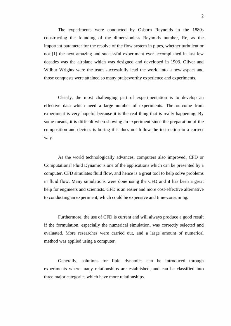
The experiments were conducted by Osborn Reynolds in the 1880s

constructing the founding of the dimensionless Reynolds number, Re, as the

important parameter for the resolve of the flow system in pipes, whether turbulent or

not [1] the next amazing and successful experiment ever accomplished in last few

decades was the airplane which was designed and developed in 1903. Oliver and

Wilbur Wrights were the team successfully lead the world into a new aspect and

those conquests were attained so many praiseworthy experience and experiments.

Clearly, the most challenging part of experimentation is to develop an

effective data which need a large number of experiments. The outcome from

experiment is very hopeful because it is the real thing that is really happening. By

some means, it is difficult when showing an experiment since the preparation of the

composition and devices is boring if it does not follow the instruction in a correct

way.

As the world technologically advances, computers also improved. CFD or

Computational Fluid Dynamic is one of the applications which can be presented by a

computer. CFD simulates fluid flow, and hence is a great tool to help solve problems

in fluid flow. Many simulations were done using the CFD and it has been a great

help for engineers and scientists. CFD is an easier and more cost-effective alternative

to conducting an experiment, which could be expensive and time-consuming.

Furthermore, the use of CFD is current and will always produce a good result

if the formulation, especially the numerical simulation, was correctly selected and

evaluated. More researches were carried out, and a large amount of numerical

method was applied using a computer.

Generally, solutions for fluid dynamics can be introduced through

experiments where many relationships are established, and can be classified into

three major categories which have more relationships.

3

Fluid

Dynamic

Solution

Experimental

CFD Theoritical

There are three different categories of solution for fluid dynamics problems:

the first one is through experiments, where the problem will be investigated in an

experimental manner and in a sample mode; the second category is a theoretical

solution, which deals with the fact that most problems dealing with fluid dynamics

have its own assumptions and mathematical equation that will result in analytical

solutions. The final category of solution is the recently generated and recently used

method known as CFD, which stands for Computational Fluid Dynamics. This

particular classification is shown in Figure 1.1

Figure 1.1 Classification of Fluid Dynamics Solution

4

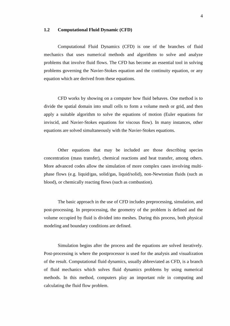
1.2 Computational Fluid Dynamic (CFD)

Computational Fluid Dynamics (CFD) is one of the branches of fluid

mechanics that uses numerical methods and algorithms to solve and analyze

problems that involve fluid flows. The CFD has become an essential tool in solving

problems governing the Navier-Stokes equation and the continuity equation, or any

equation which are derived from these equations.

CFD works by showing on a computer how fluid behaves. One method is to

divide the spatial domain into small cells to form a volume mesh or grid, and then

apply a suitable algorithm to solve the equations of motion (Euler equations for

inviscid, and Navier-Stokes equations for viscous flow). In many instances, other

equations are solved simultaneously with the Navier-Stokes equations.

Other equations that may be included are those describing species

concentration (mass transfer), chemical reactions and heat transfer, among others.

More advanced codes allow the simulation of more complex cases involving multi-

phase flows (e.g. liquid/gas, solid/gas, liquid/solid), non-Newtonian fluids (such as

blood), or chemically reacting flows (such as combustion).

The basic approach in the use of CFD includes preprocessing, simulation, and

post-processing. In preprocessing, the geometry of the problem is defined and the

volume occupied by fluid is divided into meshes. During this process, both physical

modeling and boundary conditions are defined.

Simulation begins after the process and the equations are solved iteratively.

Post-processing is where the postprocessor is used for the analysis and visualization

of the result. Computational fluid dynamics, usually abbreviated as CFD, is a branch

of fluid mechanics which solves fluid dynamics problems by using numerical

methods. In this method, computers play an important role in computing and

calculating the fluid flow problem.

5

There are many applications of CFD which are useful in the fields of

research, education, automotive, design and sports, among others. This thesis focuses

on using CFD to solve non-linear partial differential equation (PDE) where the

analytical solution typically does not exist. Regardless, some flows with analytical

solutions have applied with numerical method for validation purposes.

The base of CFD is the well-known and unsolvable non-linear incompressible

full Navier-Stokes equation. There are two types of CFD: the numerical type and

another type, which uses computer software to simulate. The second type uses a form

of software to simulate or calculate the CFD problem.

Software like FLUENT©, which is very easy to use and can be used to

simulate virtually any fluid flow problems, has some disadvantages, such as the

user’s lack of knowledge about the equations applied, the assumptions or other

criteria. This software is generally used for practical applications and for complicated

geometry and complex conditions. In spite of that, FLUENT© software is

established when it comes to numerical method but it is not publicized.

The earlier type of simulation is very notable because who create the codes

could understand the simulation, the assumption, boundary conditions and other

variables very well. This type of simulation is appropriate for information sharing

because many papers are published frequently which touts the use of new methods,

for example the Lattice Boltzmann method, Bifurcation method and CIP. The better

method is determined by carrying out comparison and validation between the

aforementioned methods. The simulation requires the user to be well-versed in

programming software such as FORTRAN, C++, and MATLAB; example

applications are the simulation of flow over cylinder [2] and the experimental [3].

6

1.2.1 Governing Equation in CFD

There are many variables and parameters in fluid flow which control the

characteristic of the flow. Generally, these parameters are related to the physics of

the flow, the nature of the fluid or the surrounding system. Some of those variables

which are usually arising in fluid flow are listed:

Temperature

Pressure

Velocity

Fluid density

Fluid viscosity, dynamic (μ) , and kinematic ( )

These are important variables in CFD simulation because they are useful and

are generally incorporated in three major governing equations. These governing

equations are very important for CFD and also for heat transfer simulation. These

equations can also be modified depending on the physics of the fluid flow or based

on the assumption which can be made. The equations involved in incompressible

fluid flow are:

The continuity equation (conservation of mass)

0. u (1.1)

The Navier-Stokes Equation (conservation of momentum)

fuvpuu 2

t .1

.u

(1.2)

The energy equation (conservation of energy)

ufupqEuEt ..)(.

(1.3)

7

The first two equations play an important role in the formulation which is

needed to produce the numerical simulation. These equations will be transferred into

a new equation based on the physical model and it is also different from one another

if the applied numerical method is different.

1.2.2 The Navier-Stokes Equations

The Navier-Stokes equations were named after the French engineer and

scientist Claude Louis Henri Navier and the English mathematical physicist George

Gabriel Stokes. The equations’ essential form was set forth by Navier in 1822;

however, the origin of viscous stress was not properly represented. The latter was

addressed by others, in particular by Poisson and Saint-Venant, but independently

developed by Stokes in 1845.

Stokes constructed a number of solutions to the equations of viscous flow,

which confirmed their ability to describe fluid dynamical phenomena.

The equation which describes the motion of fluid substances, i.e. substances

which can flow, arise from applying Newton's second law to fluid motion, together

with the assumption that the fluid stress is the sum of a diffusing viscous term

(proportional to the gradient of velocity), plus a pressure term. The mathematical

relationship which governs the fluid flow is the continuity equation and Navier-

Stokes equation given by:

0. u (1.4)

uvPuut

u 2.

(1.5)

8

With velocity u, pressure P, and kinematic shear viscosity. The Navier–

Stokes equations are a set of nonlinear partial differential equations which, unlike

algebraic υ equations, do not explicitly establish a relation among the variables of

interest (e.g. velocity and pressure). Rather, they establish relations among the rates

of change.

Navier-Stokes equation is well known in the field of fluid dynamics. The

equation is nonlinear and usually the flows that use this equation are considered

incompressible. Many fluid flows are governed by this equation because in

describing the conservation of momentum, the equation is almost perfect. In the

equation lie an unsteady term, a diffusive term, a pressure term, a convective term

and the external force which is a complete package for momentum conservation.

However, there is no analytical solution to this equation as there are many Partial

Difference term in the equation.

During the writing of this thesis, this equation is still not solved but many

types of numerical methods were tried out by scientist and engineers and hence

produce their own solution of numerical simulation. However, there still are

exceptions, because some fluid flows having the analytical solution and this

exception will be discussed later in the next chapter.

9

1.3 Problem Statement

Many classical numerical methods have been applied to investigate the

behaviors of particles in a lid-driven fluid cavity by solving the Navier-Stokes

equation accompanied with Newton’s second law and the CIP method. Yet, these

numerical methods are still insufficient; for higher order of accuracy, more grids are

needed to satisfy the methods.

Many numerical solutions are being applied to solve Navier-stokes equation

but they still lack accuracy

Low Mesh Grid has a higher accuracy.

How to properly describe the flow of a particle within a lid driven fluid

cavity.

Effect of collisions on particle flow and the trajectory of particle.

The effects of gravitational forces and drag forces and collisions on particle

flow.

1.4 Objectives of the research

The objective of this thesis is to investigate solid particles behaviors in a lid-

driven cavity flow while considering the drag force and gravitational force. In

addition, the objective is to observe the effects of collision which is divided to two

parts and will be further defined in chapters two and three. This research is mainly

based on study of the flow in a square two-dimensional cavity with particle moving

and particle collision is limited to hard sphere models only. Meanwhile, the CIP

method is applied to solve the Navier-Stokes equation to express the result with less

grid structure, which will increase the order of accuracy. The Runge-Kutta method is

used to calculate the drag force and gravitational force exerted on the particle.

10

1.5 Significance of study

Simulation allows scientists to virtually construct the experimental conditions

so that they can investigate real conditions without actually experiencing that

particular phenomenon. In some cases, it would be quite impossible to perform that

experiment with the existing facilities and defined conditions. In the field of

computational fluid dynamics, the most interesting areas in this field are description

of fluid flow and the prediction and profile of the flow.

Moreover, viscous fluids while in rotary motion have diverse industrial and

commercial applications. The main focus for researchers has been lid-driven cavity

flows, where the fluid is set into motion by part of the containing boundary. These

types of flows are tedious for analyzing fundamental aspects of recirculation fluids:

in spite of the apparently simple geometry, lid-driven cavity flows may involve a

high degree of complexity. This is an interesting problem, which may yield much

information about the interaction between fluid and particle and particle-particle and

particle-wall collisions in a wide range of practical configurations. This has not been

widely studied before this.

11

1.6 Scope of the Study

The scope for this particular research is bound by two matters and will

therefore be adhered to throughout the research, which are:

Solve the advection equation with the application of CIP for NSE by:

Comparing the results with practical and simulated benchmarks with over

other methods.

Comparing the dynamics of solid particles with the results that have been

revealed so far.

Simulating multi-particle behavior in a lid-driven cavity while considering

the effects of collision and gravitational force and drag force.

Implementation of results verification:

Two-dimensional incompressible, unsteady, lid-driven cavity.

Two-dimensional incompressible lid-driven flow in square cavity without

particle affecting, focusing on the streamline plots and velocity plots.

Two-dimensional incompressible lid-driven flow in square cavity

representing the dynamics of solid particle, focusing on the orbit of the solid

particle.

Two-dimensional incompressible lid-driven cavity flow with multiple

particles and collisions effect and gravitational force and drag force.

Particle collision is limited to Hard-Sphere model only.

Gravitational force and drag force are solved using Runge-Kutta method.

96

REFFERENCES

1. Cengel Y.A Introduction to Fluid Mechanics. 5th. ed. Singapore: Mc Graw

Hill. 2003

2. Lee K, Yang K.S Flow patterns past two circular cylinders in proximity.

Computers & Fluids , 2009. 38: 778-788.

3. Xu G, Zhou Z Strouhal numbers in the wake of two inline cylinders.

Experiments in Fluids, 2004, 37: 248-256.

4. Shankar and Deshpande, Fluid Mechanics in the Driven Cavity. Annu. Rev.

Fluid Mech, 2000: p. 32, p93.

5. Bruneau C.H., Saad M., The 2D lid-driven cavity problem

revisited,Computers & Fluids, (2006), 35 326–348.

6. Cheng M., Hung K.C, Vortex structure of steady flow in a rectangular cavity,

Computers & Fluids., (2006) 35, 1046–1062.

7. Perron S., Boivin S., Herard J.M, A finite volume method to solve the 3D

Navier Stokes equations on unstructured collocated meshes, Computers &

Fluids., (2004), 33 , 1305–1333.

8. Elman H.C.,Howle V., Shadid J.N., Tuminaro R.S., A parallel block multi-

level preconditioned for the 3D incompressible Navier Stokes equations,

Journal of Computational Physics, (2003), 187 ,504–523.

9. Zhang J, Numerical simulation of 2D square driven cavity using fourth order

compact finite difference schemes, Computers and Mathematics with

Applications .,(2003) , 45 ,43–52.

10. Auteri F., Quartapelle L, Galerkin Spectral Method for the Vorticity and

Stream Function Equations. Journal of Computational Physics, (1999), 149:

306–332.

11. Mei R., Shyy W., Yu D., Luo L.S., Lattice Boltzmann method for 3-D flows

with curved boundary, Journal of Computational Physics, (2000), 161 ,680

699.

97

12. Wright J.A., Smith R.W., An edge-based method for incompressible Navier–

Stokes equations on polygonal meshes, Journal of Computational Physics,

(2001), 169 24–43.

13. Liu C.H., Leung D.Y.C., Development of a finite element solution for the

unsteady Navier Stokes equations using projection method and fractional!

Scheme, Computer Methods in Applied Mechanics and Engineering, (2001),

190, 4301–4317.

14. Boivin S., Cayre F., Herard J.M., A finite volume method to solve the Navier-

Stokes equations for incompressible flows on unstructured meshes,

International Journal of Thermal Science, (2000), 39 ,806–825.

15. Neofytou,P.,A 3rd order upwind finite volume method for generalized

Newtonian fluid flows, Advances Engineering Software,(2005), 36, 664–680.

16. Tai C.H., Zhao Y., Liew K.M., Parallel multigrid computation of unsteady

incompressible viscous flows using a matrix-free implicit method and high

resolution characteristics based scheme, Computer Methods in Applied

Mechanics and Engineering, (2005), 194, 3949–3983.

17. Albensoeder S., Kuhlmann H.C., and Rath H.J., Multiplicity of Steady Two-

Dimensional Flows in Two-Sided Lid-Driven Cavities. Theoret. Comput.

Fluid Dynamics, (2001), 14: 223–241.

18. Albensdoer S., Kuhlmann H.C., Linear stability of rectangular cavity flows

driven by anti-parallel motion of two facing walls, Journal Of Fluid

Mechanics, (2002), 458, 153–180.

19. Albensdoer S., Kuhlmann H.C, Three dimensional instability of two counter

rotating vortices in a rectangular cavity driven by parallel wall motion,

European Journal of Mechanics B/Fluids, (2002), 21, 307–316.

20. Povitsky A., Three-dimensional flow in a cavity at yaw, Nonlinear Analysis ,

(2005), 63 1573–1584.

21. Sheu T.W.H., Tsai S.F., Flow topology in a steady three-dimensional

liddriven cavity, Computers & Fluids, (2002), 31 ,911–934.

22. Oosthuizen P.H, D. Naylor. Introduction to Convective Heat Transfer

Analysis. Singapore : Mc Graw Hill. 1999.

23. Thomas S. Applied Dimensional Analysis and Modeling. US: Elsevier, 2007.

98

24. Weinan, E. and J.G. Liu, Vorticity Boundary Condition and Related Issues

for Finite Difference Schemes. Journal of Computational Physics, 1996.

124:368–382 .

25. Tannehil J.C, Anderson D.A and Pletcher R.H. Computational Fluid

Mechanics and Heat Transfer. 2nd. ed. Taylor & Francis. 1984.

26. Takewaki H, Nishigushi A and Yabe T. Cubic Interpolated Pseudo-particle

Method (CIP) for solving Hyperbolic type equations. Journal of

Computational Physics, 1985. 61:261-268

27. Agrawal L., Mandal J.C., Marathe A.G., Computations of laminar and

turbulent mixed convection in a driven cavity using pseudo compressibility

approach, Computers & Fluids, (2001) 30 ,607–620.

28. Zhou Y., Zhang R., Staroselsky H., Chen H., Numerical simulation of

laminar and turbulent buoyancy-driven flows using a lattice Boltzmann based

algorithm, International Journal of Heat and Mass Transfer, (2004) 47

,4869–4879.

29. Alleborn N., Raszillier H., DurstF., Lid driven cavity with heat and mass

transport, International Journal of Heat and Mass Transfer,(1999) 42,833–

853.

30. Migeon C.,Texier A., Pineau G., Effects of lid-driven cavity shape on the flow

establishment phase, Journal of Fluids and Structures, (2000), 14 469 488.

31. Migeon C., Texier A. , Pineau G., Effects on Lid-driven cavity shape on the

flow establishment phase. Journal of Fluids and Structures, (2000), 14: 469-

488.

32. Tu J, Yeoh G.H, and Liu C, Computational Fluid Dynamics: A Practical

Approach. Elsevier. 2008.

33. Finnemore E.J, and Franzini J.B, Fluid Mechanics with Engineering

Application. Mc Graw Hill. 2002.

34. Grebel, W.P. Advanced Fluid Mechanics. Academic Press. 2007

35. Panton, R. L. Incompressible flow. USA : John Wiley & Son. 1984.

36. Ghia, U. Ghia, K.N. and Shin, C.T. High-Re solutions for incompressible

flow using the Navier–Stokes equations and a multigrid method. J

Computational Physics, 1982. 48: 367-411.

37. Barragy E and Carey F.C. Stream Function-Vorticity Driven Cavity Solutiion

using p Finite Elements. Computers & Fluids, 1997. 26(5): 453-468.

99

38. Albensoeder S, Kuhlmann H.C, and Rath H.J. Multiplicity of Steady Two-

Dimensional Flows in Two-Sided Lid-Driven Cavities. Theoret. Comput.

Fluid Dynamics, 2001. 14: 223–241.

39. Auteri F and Quartapelle L. Galerkin Spectral Method for the Vorticity and

Stream Function Equations. Journal of Computational Physics, 1999. 149:

306–332.

40. Tafti, D. Comparison of some upwind-biased high-order formulations with a

second-order central-difference scheme for time integration of the

incompressible Navier–Stokes equations. Computers & Fluids , 1996. 25:

647-665.

41. Botella, O. On the solution of the Navier-Stokes equations using Chebyshev

projection schemes with third-order accuracy in time. Computers and Fluids,

1997. 26: 107-116.

42. Guo Z, Shi B and Wang N. Lattice BGK Model for Incompressible Navier–

Stokes Equation. Journal of Computational Physics, 2000. 165: 288–306.

43. Migeon C, Texier A and Pineau G. Effects on Lid-driven cavity shape on the

flow establishment phase. Journal of Fluids and Structures, 2000. 14: 469-

488.

44. Anderson, J.D. Computational Fluid Dynamics: The basics with application.

Singapore : Mc Graw Hill. 1995.

45. Takewaki H, Nishigushi A and Yabe T. Cubic Interpolated Pseudo-particle

Method (CIP) for solving Hyperbolic type equations. Journal of

Computational Physics, 1985. 61:261-268

46. Yabe T, Takizawa K, Chino M, Imai M and Chu C.C. Challenge of CIP as a

universal solver for solid, liquid and gas. Int. J. Numer. Meth. Fluids, 2005.

47: 655–676.

47. Yabe T and Aoki T. A universal solver for hyperbolic-equations by cubic-

polynomial interpolation. I. One dimensional solver. Computer Physics

Communication, 1991. 66: 219-232.

48. Yabe T, Ishikawa T, Wang P.Y, Aoki T, Kadota Y and Ikeda F. A universal

solver for hyperbolic-equations by cubic-polynomial interpolation. II. Two-

and three-dimensional solvers. Computer Physics Communication, 1991. 66:

233-242.

100

49. Ogata Y, Yabe T and Odagaki K. An Accurate Numerical Scheme for

Maxwell Equation with CIP-Method of Characteristics. Communication in

Computational Physics, 2006. 1: 311-335.

50. Yabe T and Wang P.Y. Unified Numerical Procedure for Compressible and

Incompressible Fluid. Journal Physics of Society (JAPAN), 1991. 60: 2105-

2108.

51. Mizoe H , Yoon S.Y , Josho M and Yabe T. Numerical simulation on snow

melting phenomena by CIP method. Computer Physics Communications,

2001. 135: 154–166.

52. Barada D, Fukuda T, Itoh M and Yatagai T. Cubic interpolated propagation

scheme in numerical analysis of lightwave and optical force. OPTICS

EXPRESS, 2006.

53. White C.M., The equilibrium of grains on the bed of a stream, Proceedings of

the Royal Society of London. Mathematical physical sciences, (1940),332–

338.

54. Sommerfeld M., Huber N., Experimental analysis and modeling of particle–

wall collisions, International Journal of Multiphase Flow, (1999), 25 1457–

1489.

55. Sommerfeld M., Modeling of particle–wall collisions in confined gas particle

flows, International Journal of Multiphase Flow, (1992), 18 905–926.

56. Frank T., Schade K.P., Petrak D., Numerical simulation and experimental

investigation of a gas solid two phase flow in a horizontal channel,

International Journal of Multiphase Flow, (1993), 19 187–198.

57. Kuru W.C., Leighton D.T., McCready M.J., Formation of waves on a

horizontal erodible bed of particles, Journal of Multiphase Flow, (1995), 21

(6) 1123–1140.

58. Doron P., Barnea D., Pressure drop and limit deposit velocity for solid liquid

flow in pipes, Chemical Engineering Science, (1995),50 (10) 1595–1604.

59. Hayden, K.S., K. Park, and J.S. Curtis, Effect of particle characteristics on

particle pickup velocity. Powder Technology, 2003. 131(1): p. 7-14.

60. Portela L.M., Oliemans R.V.A., Eulerian Lagrangian DNS/LES of particle

turbulence interactions in wall bounded flows, International Journal for

Numerical Methods in Fluids, (2003), 26 719–727.

101

61. Crowe C, Sommerfeld M, Tsuji Y, Multiphase Flows with Droplets and

Particles, CRC Press LLC, 1998.

62. Sundaram S, Collins L.R, Numerical considerations in simulating a turbulent

suspension of finite-volume particles, Journal of Computational Physics 124

(1995) 337–350.

63. Kosinski, P., A. Kosinska, and A.C. Hoffmann., Simulation of solid particles

behaviour in a driven cavity flow. Powder Technology (2009) 191 p. 327–

339.

64. Pawel Kosinski , AlexC.Hoffmann, An extension of the hard-sphere

particle–particle collision model to study agglomeration, Chemical

Engineering Science 65 (2010) 3231–3239

65. Crowe C, Sommerfeld M, and Tsuji Y. Multiphase Flow with Droplets and

Particles. CRC Press, 1998.

66. Castellanos A, Valverde J.M, and Quintanilla M.A.S. Aggregation and

sedimentation in gas-fluidized beds of cohesive powders. Physical Review E,

64:Art. No. 041304, 2001. 67. Castellanos A, Valverde J.M, and Quintanilla M.A.S. Aggregation and

sedimentation in gas-fluidized beds of cohesive powders. Physical Review E,

64:Art. No. 041304, 2001. 68. Balakin, B., Alex C. Hoffmann, Pawel Kosinski, The collision efficiency in a

shear flow, chemical engineering science (2011) , 10.1016/2011.09.042

69. Hoomans B.P.B, Kuipers J.A.M, Briels W.J, and van Swaaij W.P.M. Discrete

particle simulation of bubble and slug formation in a two-dimensional gas-

fluidised bed: a hard sphere approach. Chem. Eng. Sci.51:99–108, 1996.

70. Visser J. An invited review: Van der Waals and other cohesive forces

affecting powder fluidization. Powder Technol., 58:1–10, 1989.

71. Brilliantov N.V, Albers N, Spahn F, and Poschel T. Collision dynamics of

granular particles with adhesion. Physical Review E, 76, 2007.

72. Tsorng S. J. ,Capart H. , Laie J. S.,Three dimensional tracking of the long

time trajectory of suspended particle in a lid driven cavity flow, experiments

in fluid , (2006) 40,314-328

73. Pawel Kosinski, Alex C. Hoffmann, An extension of the hard-sphere particle-

wall collision model to account for particle deposition, Phys. Rev. E. 79,

2009, 061302-1–061302-11