Kinematic and Dynamic Model of Robot
22
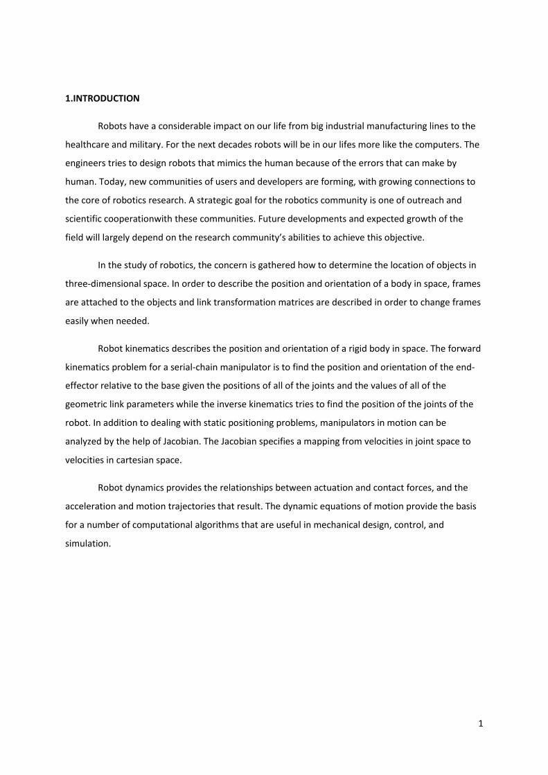
1 1.INTRODUCTION Robots have a considerable impact on our life from big industrial manufacturing lines to the healthcare and military. For the next decades robots will be in our lifes more like the computers. The engineers tries to design robots that mimics the human because of the errors that can make by human. Today, new communities of users and developers are forming, with growing connections to the core of robotics research. A strategic goal for the robotics community is one of outreach and scientific cooperationwith these communities. Future developments and expected growth of the field will largely depend on the research community’s abilities to achieve this objective. In the study of robotics, the concern is gathered how to determine the location of objects in three-dimensional space. In order to describe the position and orientation of a body in space, frames are attached to the objects and link transformation matrices are described in order to change frames easily when needed. Robot kinematics describes the position and orientation of a rigid body in space. The forward kinematics problem for a serial-chain manipulator is to find the position and orientation of the end- effector relative to the base given the positions of all of the joints and the values of all of the geometric link parameters while the inverse kinematics tries to find the position of the joints of the robot. In addition to dealing with static positioning problems, manipulators in motion can be analyzed by the help of Jacobian. The Jacobian specifies a mapping from velocities in joint space to velocities in cartesian space. Robot dynamics provides the relationships between actuation and contact forces, and the acceleration and motion trajectories that result. The dynamic equations of motion provide the basis for a number of computational algorithms that are useful in mechanical design, control, and simulation.
-
Upload
ismail-kayahan -
Category
Documents
-
view
55 -
download
0
description
determine the location of objects inthree-dimensional space. In order to describe the position and orientation of a body in space, framesare attached to the objects and link transformation matrices are described in order to change frameseasily when needed.
Transcript of Kinematic and Dynamic Model of Robot
1
1.INTRODUCTION
Robots have a considerable impact on our life from big industrial manufacturing lines to the
healthcare and military. For the next decades robots will be in our lifes more like the computers. The
engineers tries to design robots that mimics the human because of the errors that can make by
human. Today, new communities of users and developers are forming, with growing connections to
the core of robotics research. A strategic goal for the robotics community is one of outreach and
scientific cooperationwith these communities. Future developments and expected growth of the
field will largely depend on the research community’s abilities to achieve this objective.
In the study of robotics, the concern is gathered how to determine the location of objects in
three-dimensional space. In order to describe the position and orientation of a body in space, frames
are attached to the objects and link transformation matrices are described in order to change frames
easily when needed.
Robot kinematics describes the position and orientation of a rigid body in space. The forward
kinematics problem for a serial-chain manipulator is to find the position and orientation of the end-
effector relative to the base given the positions of all of the joints and the values of all of the
geometric link parameters while the inverse kinematics tries to find the position of the joints of the
robot. In addition to dealing with static positioning problems, manipulators in motion can be
analyzed by the help of Jacobian. The Jacobian specifies a mapping from velocities in joint space to
velocities in cartesian space.
Robot dynamics provides the relationships between actuation and contact forces, and the
acceleration and motion trajectories that result. The dynamic equations of motion provide the basis
for a number of computational algorithms that are useful in mechanical design, control, and
simulation.
2
2.DESCRIPTION OF THE ROBOT
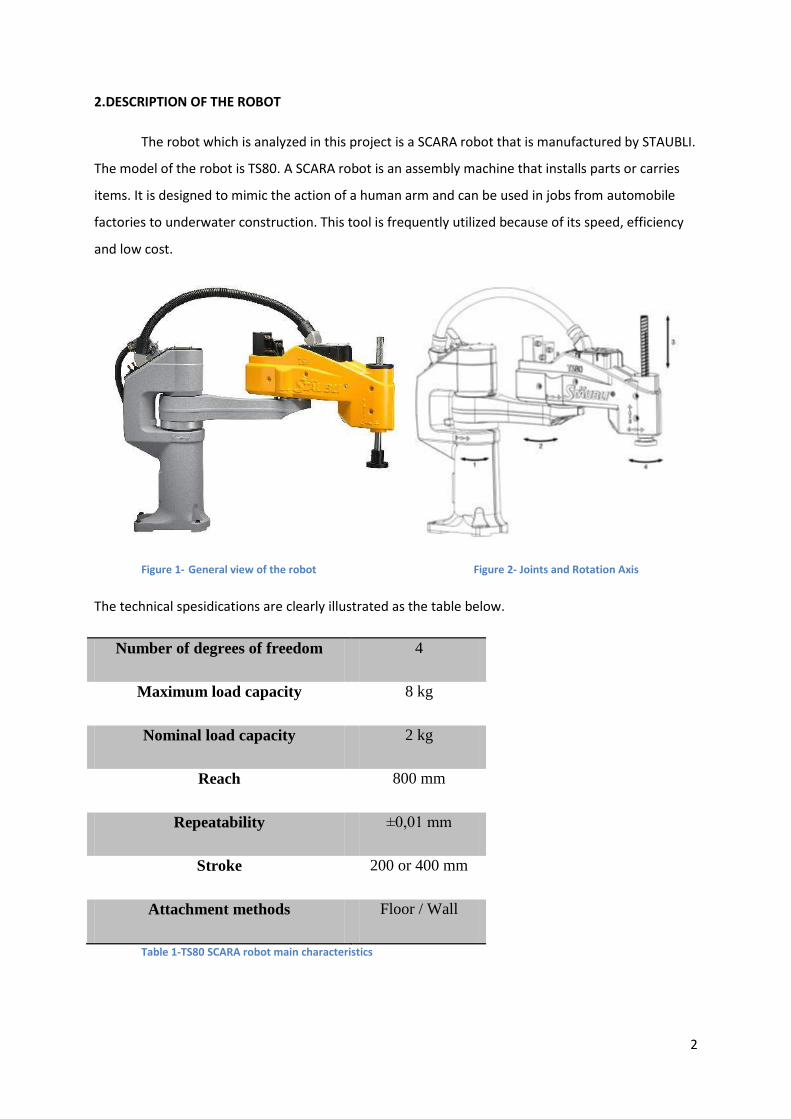
The robot which is analyzed in this project is a SCARA robot that is manufactured by STAUBLI.
The model of the robot is TS80. A SCARA robot is an assembly machine that installs parts or carries
items. It is designed to mimic the action of a human arm and can be used in jobs from automobile
factories to underwater construction. This tool is frequently utilized because of its speed, efficiency
and low cost.
Figure 1- General view of the robot Figure 2- Joints and Rotation Axis
The technical spesidications are clearly illustrated as the table below.
Number of degrees of freedom 4
Maximum load capacity 8 kg
Nominal load capacity 2 kg
Reach 800 mm
Repeatability ±0,01 mm
Stroke 200 or 400 mm
Attachment methods Floor / Wall
Table 1-TS80 SCARA robot main characteristics
3
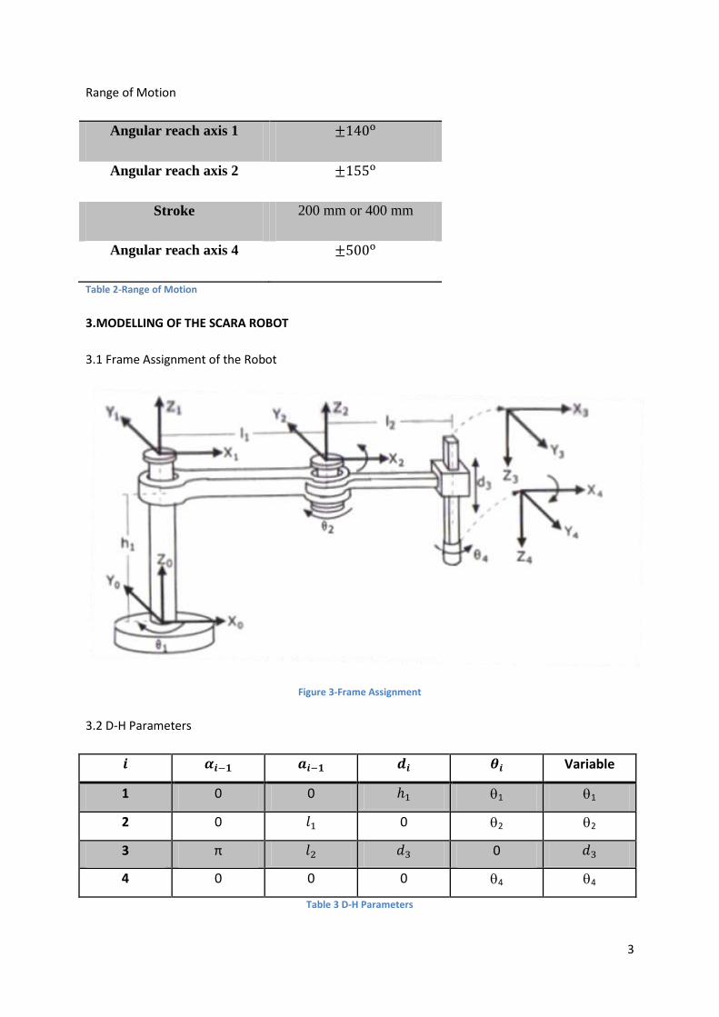
Range of Motion
Angular reach axis 1
Angular reach axis 2
Stroke 200 mm or 400 mm
Angular reach axis 4
Table 2-Range of Motion
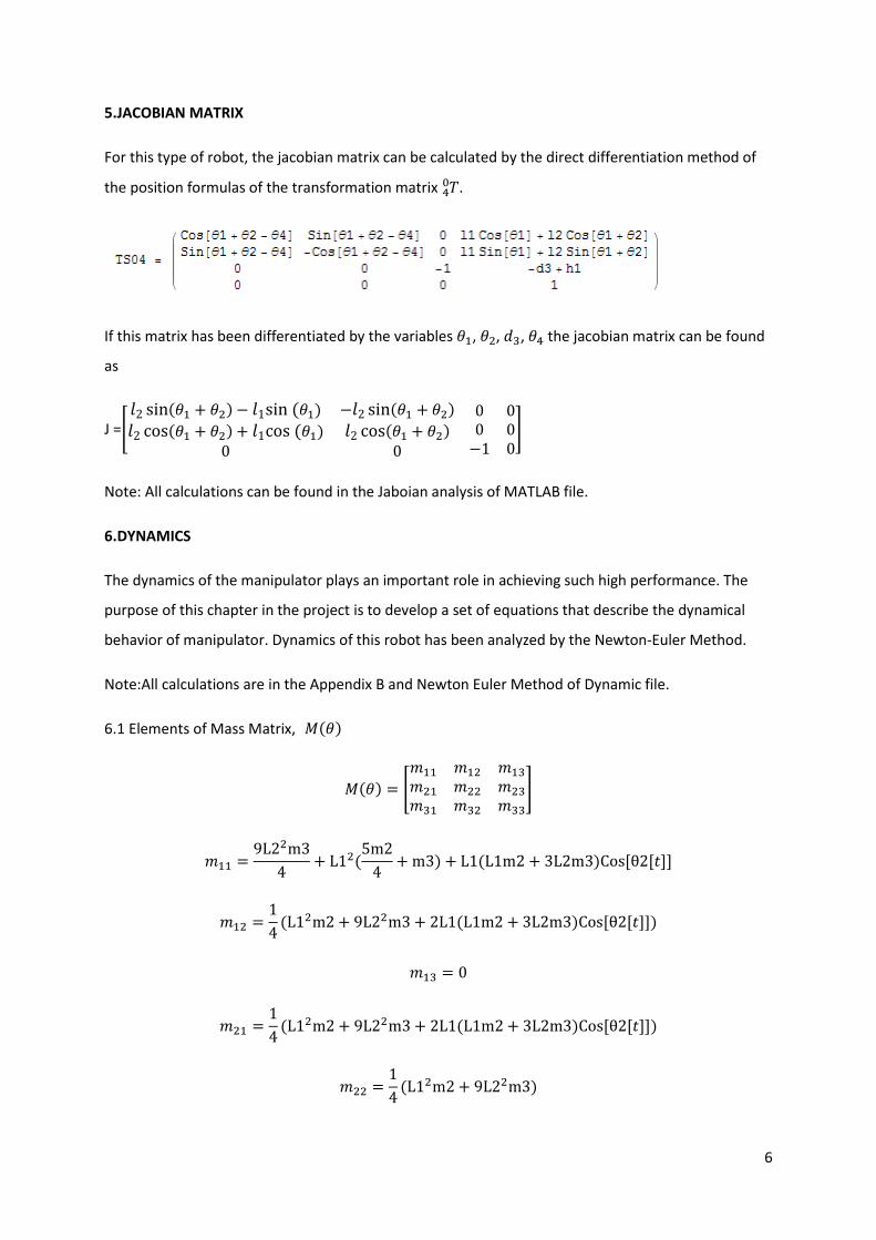
3.MODELLING OF THE SCARA ROBOT
3.1 Frame Assignment of the Robot
Figure 3-Frame Assignment
3.2 D-H Parameters
Variable
1 0 0 1 1
2 0 0 2 2
3 π 0
4 0 0 0 4 4
Table 3 D-H Parameters

4
3.3Transformation Matrices
4.KINEMATIC ANALYSIS OF ROBOT
4.1 Forward Kinematics
r 1 1 = Cos[1+2-4]
r 1 2 = Sin[1+2-4]
r 1 3 = 0
r 2 1 = Sin[1+2-4]
r 2 2 = -Cos[1+2-4]
r 2 3 = 0
r 3 1 = 0
r 3 2 = 0

5
r 3 3 = -1
px= (l1 Cos[1]+l2 Cos[1+2])
py= (l1 Sin[1]+l2 Sin[1+2])
pz= (-d3+h1)
Note: Detailed information in the Kinematic Analysis of Robot Mathematica file.
4.2 Inverse Kinematics:
1- From the forward kinematic analysis px and py can be calculated as follows;
Where
2- Choose [2,4]
)
3- Choose [3,4]
4-Choose [1,1] ,
[1,2]
Note: Detailed information in the Appendix A and Kinematic Analysis of Robot Mathematica
file.
6
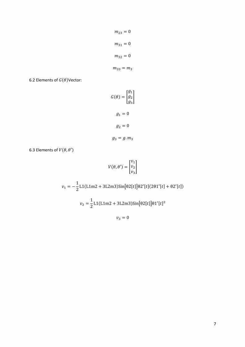
5.JACOBIAN MATRIX
For this type of robot, the jacobian matrix can be calculated by the direct differentiation method of
the position formulas of the transformation matrix .
If this matrix has been differentiated by the variables , , , the jacobian matrix can be found
as
J =
Note: All calculations can be found in the Jaboian analysis of MATLAB file.
6.DYNAMICS
The dynamics of the manipulator plays an important role in achieving such high performance. The
purpose of this chapter in the project is to develop a set of equations that describe the dynamical
behavior of manipulator. Dynamics of this robot has been analyzed by the Newton-Euler Method.
Note:All calculations are in the Appendix B and Newton Euler Method of Dynamic file.
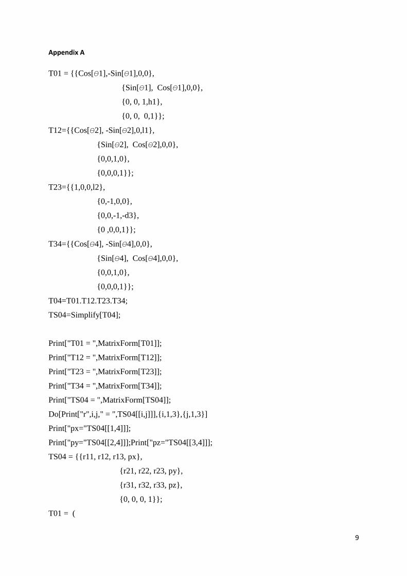
6.1 Elements of Mass Matrix,
7
6.2 Elements of Vector:
6.3 Elements of

8
7.CONCLUSION
In this project, at the first part the description of the robot is defined and the properties is clearly
showed to clearly state the robot. After this descriptions, modeling of the robot part is prepared. In
this part firstly frames are assigned and joints are determined that which are prismatic and revolute.
With this assignments the Denavit-Hartenberg parameters table is created to generate the
transformation matrices of the links.
After the generation of the transformation matrices of all links with respect to the previous one,
forward kinematics which is calculated to find the end-effector position is solved by the help of the
Mathematica software.
Then the inverse kinematics is calculated to find the joints position of the robot while the end-
effector position is known. Most of the mathematical operations at this part is made by hand
because of the trigonometric equations of the end-effector position formulations.
For determination of the velocities of the joints jacobian matrix is calculated by the direct derivation
method. The position equations of transformation matrix of robot’s is derivate by all the variables of
the robot. For the calculations of this part MATLAB is used and the codes for the calculations is stated
in the appendix part.
Furthermore, the dynamic analysis can be made by different methods like Newton-Euler or
Lagrangian. All of the methods generates the same results but in different forms of equation sets. In
this project Newton-Euler Method is chosen which uses a Newton–Euler formulation of the
problem,and is based on the very efficient recursive Newton–Euler algorithm. At this part
Mathematica software is used.
REFERENCES
Bruno Siciliano, Oussama Khatib, Handbook of Robotics,Springer,2008
Mahdi Salman Alshamasin, Florin Ionescu, Kinematic Modeling and Simulation of a SCARA
Robot by Using Solid Dynamics and Verification by MATLAB/Simulink, European Journal of
Scientific Research, Vol.37 No.3 (2009), pp.388-405
John J.Craig,”Introduction To Robotics”,Prentice Hall,2005
Lung-Wen Tsai,Robot analysis : the mechanics of serial and parallel manipulators, Wiley,1999
9
Appendix A
T01 = {{Cos[1],-Sin[1],0,0},
{Sin[1], Cos[1],0,0},
{0, 0, 1,h1},
{0, 0, 0,1}};
T12={{Cos[2], -Sin[2],0,l1},
{Sin[2], Cos[2],0,0},
{0,0,1,0},
{0,0,0,1}};
T23={{1,0,0,l2},
{0,-1,0,0},
{0,0,-1,-d3},
{0 ,0,0,1}};
T34={{Cos[4], -Sin[4],0,0},
{Sin[4], Cos[4],0,0},
{0,0,1,0},
{0,0,0,1}};
T04=T01.T12.T23.T34;
TS04=Simplify[T04];
Print["T01 = ",MatrixForm[T01]];
Print["T12 = ",MatrixForm[T12]];
Print["T23 = ",MatrixForm[T23]];
Print["T34 = ",MatrixForm[T34]];
Print["TS04 = ",MatrixForm[TS04]];
Do[Print["r",i,j," = ",TS04[[i,j]]],{i,1,3},{j,1,3}]
Print["px="TS04[[1,4]]];
Print["py="TS04[[2,4]]];Print["pz="TS04[[3,4]]];
TS04 = {{r11, r12, r13, px},
{r21, r22, r23, py},
{r31, r32, r33, pz},
{0, 0, 0, 1}};
T01 = (
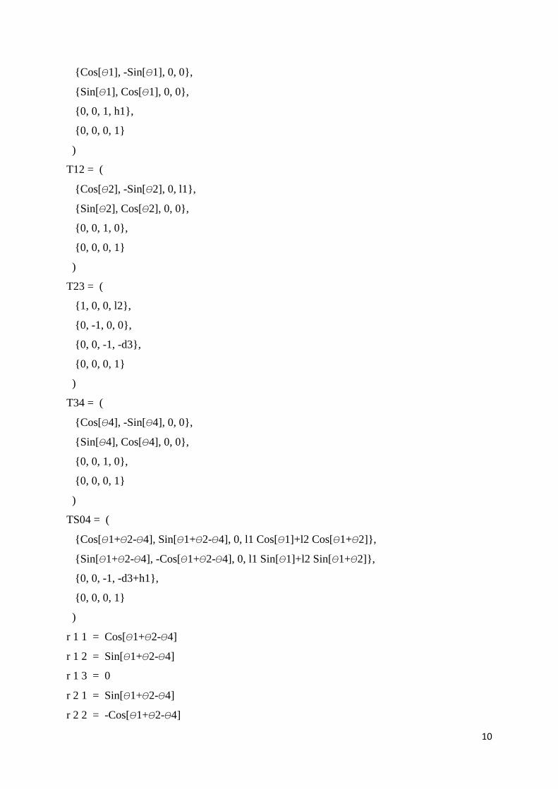
10
{Cos[1], -Sin[1], 0, 0},
{Sin[1], Cos[1], 0, 0},
{0, 0, 1, h1},
{0, 0, 0, 1}
)
T12 = (
{Cos[2], -Sin[2], 0, l1},
{Sin[2], Cos[2], 0, 0},
{0, 0, 1, 0},
{0, 0, 0, 1}
)
T23 = (
{1, 0, 0, l2},
{0, -1, 0, 0},
{0, 0, -1, -d3},
{0, 0, 0, 1}
)
T34 = (
{Cos[4], -Sin[4], 0, 0},
{Sin[4], Cos[4], 0, 0},
{0, 0, 1, 0},
{0, 0, 0, 1}
)
TS04 = (
{Cos[1+2-4], Sin[1+2-4], 0, l1 Cos[1]+l2 Cos[1+2]},
{Sin[1+2-4], -Cos[1+2-4], 0, l1 Sin[1]+l2 Sin[1+2]},
{0, 0, -1, -d3+h1},
{0, 0, 0, 1}
)
r 1 1 = Cos[1+2-4]
r 1 2 = Sin[1+2-4]
r 1 3 = 0
r 2 1 = Sin[1+2-4]
r 2 2 = -Cos[1+2-4]

11
r 2 3 = 0
r 3 1 = 0
r 3 2 = 0
r 3 3 = -1
px= (l1 Cos[1]+l2 Cos[1+2])
py= (l1 Sin[1]+l2 Sin[1+2])
pz= (-d3+h1)
RST14 = Simplify[T12.T23.T34]
Do[Print["RST14[",i,",",j,"] = ",RST14[[i,j]]],{i,1,4},{j,1,4}]
{{Cos[2-4],Sin[2-4],0,l1+l2 Cos[2]},{Sin[2-4],-Cos[2-4],0,l2 Sin[2]},{0,0,-1,-
d3},{0,0,0,1}}
RST14[ 1 , 1 ] = Cos[2-4]
RST14[ 1 , 2 ] = Sin[2-4]
RST14[ 1 , 3 ] = 0
RST14[ 1 , 4 ] = l1+l2 Cos[2]
RST14[ 2 , 1 ] = Sin[2-4]
RST14[ 2 , 2 ] = -Cos[2-4]
RST14[ 2 , 3 ] = 0
RST14[ 2 , 4 ] = l2 Sin[2]
RST14[ 3 , 1 ] = 0
RST14[ 3 , 2 ] = 0
RST14[ 3 , 3 ] = -1
RST14[ 3 , 4 ] = -d3
RST14[ 4 , 1 ] = 0
RST14[ 4 , 2 ] = 0
RST14[ 4 , 3 ] = 0
RST14[ 4 , 4 ] = 1
LST14 =Simplify[Inverse[T01]].TS04;
Do[Print["LST14[",i,",",j,"] = ",LST14[[i,j]]],{i,1,4},{j,1,4}]
LST14[ 1 , 1 ] = r11 Cos[1]+r21 Sin[1]
LST14[ 1 , 2 ] = r12 Cos[1]+r22 Sin[1]
LST14[ 1 , 3 ] = r13 Cos[1]+r23 Sin[1]
LST14[ 1 , 4 ] = px Cos[1]+py Sin[1]
LST14[ 2 , 1 ] = r21 Cos[1]-r11 Sin[1]

12
LST14[ 2 , 2 ] = r22 Cos[1]-r12 Sin[1]
LST14[ 2 , 3 ] = r23 Cos[1]-r13 Sin[1]
LST14[ 2 , 4 ] = py Cos[1]-px Sin[1]
LST14[ 3 , 1 ] = r31
LST14[ 3 , 2 ] = r32
LST14[ 3 , 3 ] = r33
LST14[ 3 , 4 ] = -h1+pz
LST14[ 4 , 1 ] = 0
LST14[ 4 , 2 ] = 0
LST14[ 4 , 3 ] = 0
LST14[ 4 , 4 ] = 1
RST24 = Simplify[T23.T34];
Do[Print["RST24[",i,",",j,"] = ",RST24[[i,j]]],{i,1,4},{j,1,4}]
RST24[ 1 , 1 ] = Cos[4]
RST24[ 1 , 2 ] = -Sin[4]
RST24[ 1 , 3 ] = 0
RST24[ 1 , 4 ] = l2
RST24[ 2 , 1 ] = -Sin[4]
RST24[ 2 , 2 ] = -Cos[4]
RST24[ 2 , 3 ] = 0
RST24[ 2 , 4 ] = 0
RST24[ 3 , 1 ] = 0
RST24[ 3 , 2 ] = 0
RST24[ 3 , 3 ] = -1
RST24[ 3 , 4 ] = -d3
RST24[ 4 , 1 ] = 0
RST24[ 4 , 2 ] = 0
RST24[ 4 , 3 ] = 0
RST24[ 4 , 4 ] = 1
T02=T01.T12;
LST24 =Simplify[Inverse[T02]].TS04;
Do[Print["LST24[",i,",",j,"] = ",LST24[[i,j]]],{i,1,4},{j,1,4}]
LST24[ 1 , 1 ] = r11 Cos[1+2]+r21 Sin[1+2]
LST24[ 1 , 2 ] = r12 Cos[1+2]+r22 Sin[1+2]

13
LST24[ 1 , 3 ] = r13 Cos[1+2]+r23 Sin[1+2]
LST24[ 1 , 4 ] = -l1 Cos[2]+px Cos[1+2]+py Sin[1+2]
LST24[ 2 , 1 ] = r21 Cos[1+2]-r11 Sin[1+2]
LST24[ 2 , 2 ] = r22 Cos[1+2]-r12 Sin[1+2]
LST24[ 2 , 3 ] = r23 Cos[1+2]-r13 Sin[1+2]
LST24[ 2 , 4 ] = py Cos[1+2]+l1 Sin[2]-px Sin[1+2]
LST24[ 3 , 1 ] = r31
LST24[ 3 , 2 ] = r32
LST24[ 3 , 3 ] = r33
LST24[ 3 , 4 ] = -h1+pz
LST24[ 4 , 1 ] = 0
LST24[ 4 , 2 ] = 0
LST24[ 4 , 3 ] = 0
LST24[ 4 , 4 ] = 1
RST34 = Simplify[T34]
Do[Print["RST34[",i,",",j,"] = ",RST34[[i,j]]],{i,1,4},{j,1,4}]
{{Cos[4],-Sin[4],0,0},{Sin[4],Cos[4],0,0},{0,0,1,0},{0,0,0,1}}
RST34[ 1 , 1 ] = Cos[4]
RST34[ 1 , 2 ] = -Sin[4]
RST34[ 1 , 3 ] = 0
RST34[ 1 , 4 ] = 0
RST34[ 2 , 1 ] = Sin[4]
RST34[ 2 , 2 ] = Cos[4]
RST34[ 2 , 3 ] = 0
RST34[ 2 , 4 ] = 0
RST34[ 3 , 1 ] = 0
RST34[ 3 , 2 ] = 0
RST34[ 3 , 3 ] = 1
RST34[ 3 , 4 ] = 0
RST34[ 4 , 1 ] = 0
RST34[ 4 , 2 ] = 0
RST34[ 4 , 3 ] = 0
RST34[ 4 , 4 ] = 1
T03=T01.T12.T23;

14
LST34 =Simplify[Inverse[T03]].TS04;
Do[Print["LST34[",i,",",j,"] = ",LST34[[i,j]]],{i,1,4},{j,1,4}]
LST34[ 1 , 1 ] = r11 Cos[1+2]+r21 Sin[1+2]
LST34[ 1 , 2 ] = r12 Cos[1+2]+r22 Sin[1+2]
LST34[ 1 , 3 ] = r13 Cos[1+2]+r23 Sin[1+2]
LST34[ 1 , 4 ] = -l2-l1 Cos[2]+px Cos[1+2]+py Sin[1+2]
LST34[ 2 , 1 ] = -r21 Cos[1+2]+r11 Sin[1+2]
LST34[ 2 , 2 ] = -r22 Cos[1+2]+r12 Sin[1+2]
LST34[ 2 , 3 ] = -r23 Cos[1+2]+r13 Sin[1+2]
LST34[ 2 , 4 ] = -py Cos[1+2]-l1 Sin[2]+px Sin[1+2]
LST34[ 3 , 1 ] = -r31
LST34[ 3 , 2 ] = -r32
LST34[ 3 , 3 ] = -r33
LST34[ 3 , 4 ] = -d3+h1-pz
LST34[ 4 , 1 ] = 0
LST34[ 4 , 2 ] = 0
LST34[ 4 , 3 ] = 0
LST34[ 4 , 4 ] = 1
Appendix B
syms Q1
syms Q2
syms d3
syms Q4
syms l1
syms l2
syms h1
px=l1*cos(Q1)+l2*cos(Q1+Q2);
py=(l1*sin(Q1)+l2*sin(Q1+Q2));
15
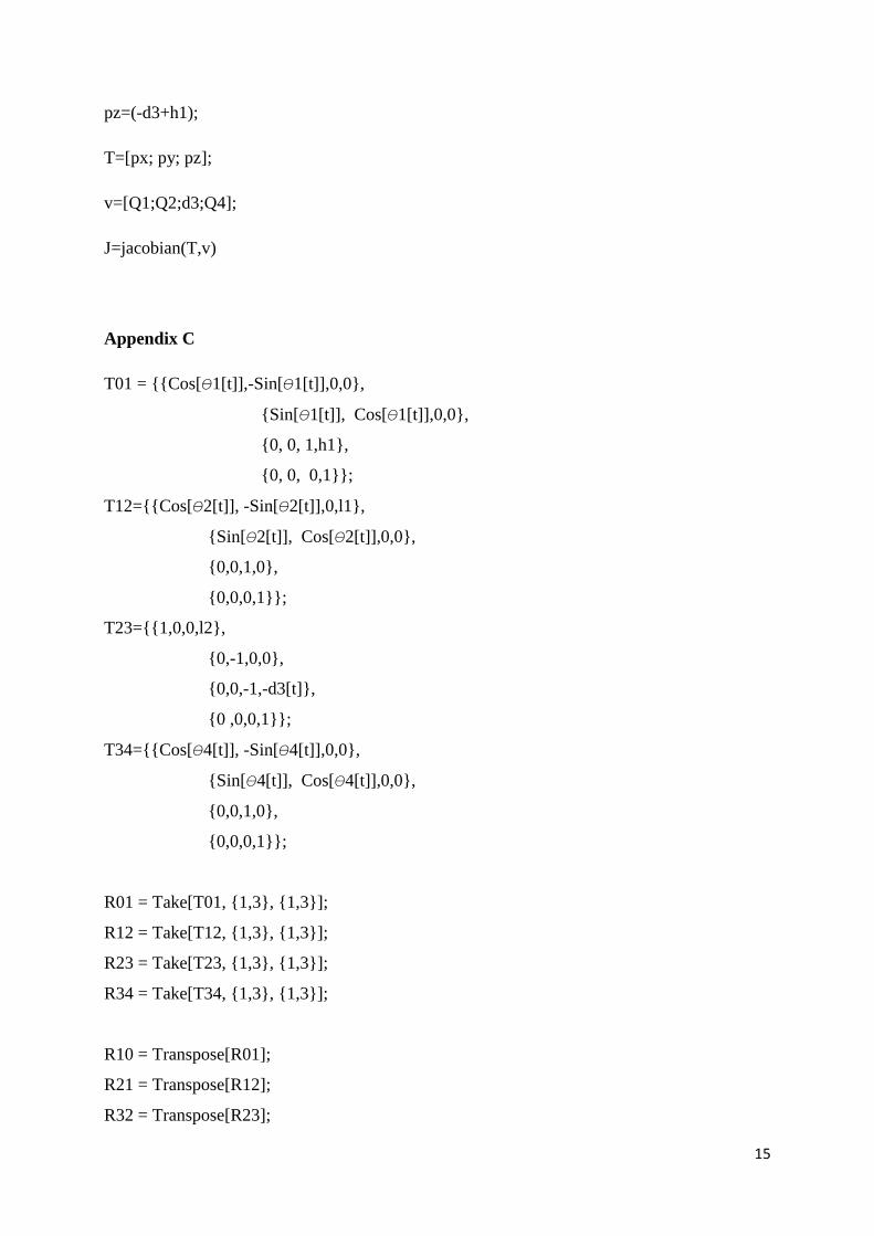
pz=(-d3+h1);
T=[px; py; pz];
v=[Q1;Q2;d3;Q4];
J=jacobian(T,v)
Appendix C
T01 = {{Cos[1[t]],-Sin[1[t]],0,0},
{Sin[1[t]], Cos[1[t]],0,0},
{0, 0, 1,h1},
{0, 0, 0,1}};
T12={{Cos[2[t]], -Sin[2[t]],0,l1},
{Sin[2[t]], Cos[2[t]],0,0},
{0,0,1,0},
{0,0,0,1}};
T23={{1,0,0,l2},
{0,-1,0,0},
{0,0,-1,-d3[t]},
{0 ,0,0,1}};
T34={{Cos[4[t]], -Sin[4[t]],0,0},
{Sin[4[t]], Cos[4[t]],0,0},
{0,0,1,0},
{0,0,0,1}};
R01 = Take[T01, {1,3}, {1,3}];
R12 = Take[T12, {1,3}, {1,3}];
R23 = Take[T23, {1,3}, {1,3}];
R34 = Take[T34, {1,3}, {1,3}];
R10 = Transpose[R01];
R21 = Transpose[R12];
R32 = Transpose[R23];

16
R43 = Transpose[R34];
Center of Mass Vectors:
P1c1 = {0, 0, h1/2};
P2c2 = {L1/2, 0, 0};
P3c3 = {L2/2, 0, 0};
P4c4 = {0, 0, -d3[t]/2};
Frame-to-Frame Vectors:
P01 = {0,0,h1};
P12 = {L1, 0,0};
P23 = {L2, 0, 0};
P34 = {0, 0, d3[t]};
Forces/Moments at End Effector:
f44= {0,0,0};
n44 = {0,0,0};
Angular Velocity and Acceleration and Linear
Acceleration of Base:
00 = {0,0,0};
00' = {0,0,0};
v00' = {0,0,-g};
Inertia Tensors
Ic11 = {{0,0,0},
{0,0,0},
{0,0,0}};
Ic22 = {{0,0,0},

17
{0,0,0},
{0,0,0}};
Ic33= {{0,0,0},
{0,0,0},
{0,0,0}};
Ic44 = {{0,0,0},
{0,0,0},
{0,0,0}};
Outward Iterations for Link 1 (Revolute):
11 = R10.00+{0,0,1'[t]}
{0,0,1[t]}
11' = R10.00'+{0,0,1''[t]}+Cross[R10.00,{0,0,1'[t]}]
{0,0,1[t]}
v11' = R10.(Cross[00',P01]+Cross[00,Cross[00,P01]]+v00')
{0,0,-g}
vc11' = Cross[11',P1c1]+Cross[11, Cross[11,P1c1]]+v11'
{0,0,-g}
F11 = m1 (vc11')
{0,0,-g m1}
N11 = Ic11.11'+Cross[11,Ic11.11]
{0,0,0}
Outward Iterations for Link 2 (Revolute) :
22 = R21.11+{0,0,2'[t]}
{0,0,1[t]+2[t]}
22' = R21.11'+{0,0,2''[t]}+Cross[R21.11,{0,0,2'[t]}]
{0,0,1[t]+2[t]}
v22' = Simplify[R21.(Cross[11',P12]+Cross[11,Cross[11,P12]]+v11')]
{-L1 Cos[2[t]] (1^)[t]2+L1 Sin[2[t]] 1
[t],L1 (Sin[2[t]] (1^)[t]2+Cos[2[t]] 1
[t]),-g}

18
vc22' =Simplify[ Cross[22',P2c2]+Cross[22, Cross[22,P2c2]]+v22']
{-(1/2) L1 ((1+2 Cos[2[t]]) (1^)[t]2+2 1
[t] 2[t]+(2^)[t]2-2 Sin[2[t]] 1
[t]),1/2 L1 (2 Sin[2[t]]
(1^)[t]2+(1+2 Cos[2[t]]) 1
[t]+2[t]),-g}
F22 = m2 (vc22')
{-(1/2) L1 m2 ((1+2 Cos[2[t]]) (1^)[t]2+2 1
[t] 2[t]+(2^)[t]2-2 Sin[2[t]] 1
[t]),1/2 L1 m2 (2
Sin[2[t]] (1^)[t]2+(1+2 Cos[2[t]]) 1
[t]+2[t]),-g m2}
N22 = Ic22.22'+Cross[22,Ic22.22]
{0,0,0}
Outward Iterations for Link 3 (Prismatic) :
33 = R32.22
{0,0,-1[t]-2[t]}
33'=R32.22'
{0,0,-1[t]-2[t]}
v33' =
Simplify[R32.(Cross[22',P23]+Cross[22,Cross[22,P23]]+v22')+2.Cross[33,{0,0,d3'[t]}]
+{0,0,d3''[t]}]
{-(L2+L1 Cos[2[t]]) (1^)[t]2-2 L2 1
[t] 2[t]-L2 (2^)[t]2+L1 Sin[2[t]] 1
[t],-L1 Sin[2[t]]
(1^)[t]2-(L2+L1 Cos[2[t]]) 1
[t]-L2 2[t],g+d3[t]}
vc33' =Simplify[ Cross[{0,0,-1[t]-2[t]},P3c3]+Cross[33, Cross[33,P3c3]]+v33']
{-(1/2) (3 L2+2 L1 Cos[2[t]]) (1^)[t]2-3 L2 1
[t] 2[t]-3/2 L2 (2^)[t]2+L1 Sin[2[t]] 1
[t],1/2 (-
2 L1 Sin[2[t]] (1^)[t]2-(3 L2+2 L1 Cos[2[t]]) 1
[t]-3 L2 2[t]),g+d3[t]}
F33 = m3 (vc33')
{m3 (-(1/2) (3 L2+2 L1 Cos[2[t]]) (1^)[t]2-3 L2 1
[t] 2[t]-3/2 L2 (2^)[t]2+L1 Sin[2[t]]
1[t]),1/2 m3 (-2 L1 Sin[2[t]] (1^)[t]2
-(3 L2+2 L1 Cos[2[t]]) 1[t]-3 L2 2[t]),m3 (g+d3[t])}
N33= Ic33.{0,0,-1[t]-2[t]}+Cross[33,Ic33.33]
{0,0,0}
Outward Iterations for Link 4 (Revolute) :
44 = R43.33+{0,0,4'[t]}
{0,0,-1[t]-2[t]+4[t]}

19
44' = R43.{0,0,-1[t]-2[t]}+{0,0,4''[t]}+Cross[R43.33,{0,0,4'[t]}]
{0,0,-1[t]-2[t]+4[t]}
v44' = Simplify[R43.(Cross[{0,0,-1[t]-2[t]},P34]+Cross[33,Cross[33,P34]]+v33')]
{Cos[4[t]] (-(L2+L1 Cos[2[t]]) (1^)[t]2-2 L2 1
[t] 2[t]-L2 (2^)[t]2+L1 Sin[2[t]] 1
[t])-
Sin[4[t]] (L1 Sin[2[t]] (1^)[t]2+(L2+L1 Cos[2[t]]) 1
[t]+L2 2[t]),(-L1 Sin[2[t]-4[t]]+L2 Sin[4[t]])
(1^)[t]2+2 L2 Sin[4[t]] 1
[t] 2[t]+L2 Sin[4[t]] (2^)[t]2-L1 Cos[2[t]-4[t]] 1
[t]-L2 Cos[4[t]] 1[t]-
L2 Cos[4[t]] 2[t],g+d3[t]}
vc44' =Simplify[ Cross[44',P4c4]+Cross[44, Cross[44,P4c4]]+v44']
{Cos[4[t]] (-(L2+L1 Cos[2[t]]) (1^)[t]2-2 L2 1
[t] 2[t]-L2 (2^)[t]2+L1 Sin[2[t]] 1
[t])-
Sin[4[t]] (L1 Sin[2[t]] (1^)[t]2+(L2+L1 Cos[2[t]]) 1
[t]+L2 2[t]),(-L1 Sin[2[t]-4[t]]+L2 Sin[4[t]])
(1^)[t]2+2 L2 Sin[4[t]] 1
[t] 2[t]+L2 Sin[4[t]] (2^)[t]2-L1 Cos[2[t]-4[t]] 1
[t]-L2 Cos[4[t]] 1[t]-
L2 Cos[4[t]] 2[t],g+d3[t]}
F44 = m4 (vc44')
{m4 (Cos[4[t]] (-(L2+L1 Cos[2[t]]) (1^)[t]2-2 L2 1
[t] 2[t]-L2 (2^)[t]2+L1 Sin[2[t]]
1[t])-Sin[4[t]] (L1 Sin[2[t]] (1^)[t]2
+(L2+L1 Cos[2[t]]) 1[t]+L2 2[t])),m4 ((-L1 Sin[2[t]-4[t]]+L2
Sin[4[t]]) (1^)[t]2+2 L2 Sin[4[t]] 1
[t] 2[t]+L2 Sin[4[t]] (2^)[t]2-L1 Cos[2[t]-4[t]] 1
[t]-L2
Cos[4[t]] 1[t]-L2 Cos[4[t]] 2[t]),m4 (g+d3[t])}
N44 = Ic44.44'+Cross[44,Ic44.44]
{0,0,0}
Inward Iterations for Link 3
f33 = R34.f44+F33
{m3 (-(1/2) (3 L2+2 L1 Cos[2[t]]) (1^)[t]2-3 L2 1
[t] 2[t]-3/2 L2 (2^)[t]2+L1 Sin[2[t]]
1[t]),1/2 m3 (-2 L1 Sin[2[t]] (1^)[t]2
-(3 L2+2 L1 Cos[2[t]]) 1[t]-3 L2 2[t]),m3 (g+d3[t])}
n33 = N33+R34.n44+Cross[P3c3,F33]+Cross[P34,R34.f44]
{0,-(1/2) g L2 m3-1/2 L2 m3 d3[t],-(1/2) L1 L2 m3 Sin[2[t]] (1^)[t]2
-3/4 L22 m3 1
[t]-1/2 L1 L2 m3
Cos[2[t]] 1[t]-3/4 L22 m3 2
[t]}
Inward Iterations for Link 2
f22 = R23.f33+F22

20
{-(1/2) L1 m2 ((1+2 Cos[2[t]]) (1^)[t]2+2 1
[t] 2[t]+(2^)[t]2-2 Sin[2[t]] 1
[t])+m3 (-(1/2) (3
L2+2 L1 Cos[2[t]]) (1^)[t]2-3 L2 1
[t] 2[t]-3/2 L2 (2^)[t]2+L1 Sin[2[t]] 1
[t]),1/2 L1 m2 (2 Sin[2[t]]
(1^)[t]2+(1+2 Cos[2[t]]) 1
[t]+2[t])-1/2 m3 (-2 L1 Sin[2[t]] (1^)[t]2-(3 L2+2 L1 Cos[2[t]]) 1
[t]-3
L2 2[t]),-g m2-m3 (g+d3[t])}
n22 = N22+R23.n33+Cross[P2c2,F22]+Cross[P23,R23.f33]
{0,(g L1 m2)/2+(3 g L2 m3)/2+3/2 L2 m3 d3[t],1/2 L12
m2 Sin[2[t]] (1^)[t]2+3/2 L1 L2 m3
Sin[2[t]] (1^)[t]2+1/4 L1
2 m2 1
[t]+9/4 L22 m3 1
[t]+1/2 L12 m2 Cos[2[t]] 1
[t]+3/2 L1 L2 m3
Cos[2[t]] 1[t]+1/4 L12 m2 2
[t]+9/4 L22 m3 2
[t]}
Inward Iterations for Link 1
f11 = R12.f22+F11
{Cos[2[t]] (-(1/2) L1 m2 ((1+2 Cos[2[t]]) (1^)[t]2+2 1
[t] 2[t]+(2^)[t]2-2 Sin[2[t]]
1[t])+m3 (-(1/2) (3 L2+2 L1 Cos[2[t]]) (1^)[t]2
-3 L2 1[t] 2[t]-3/2 L2 (2^)[t]2
+L1 Sin[2[t]] 1[t]))-Sin[2[t]]
(1/2 L1 m2 (2 Sin[2[t]] (1^)[t]2+(1+2 Cos[2[t]]) 1
[t]+2[t])-1/2 m3 (-2 L1 Sin[2[t]] (1^)[t]2-(3 L2+2 L1
Cos[2[t]]) 1[t]-3 L2 2[t])),Sin[2[t]] (-(1/2) L1 m2 ((1+2 Cos[2[t]]) (1^)[t]2
+2 1[t] 2[t]+(2^)[t]2
-2
Sin[2[t]] 1[t])+m3 (-(1/2) (3 L2+2 L1 Cos[2[t]]) (1^)[t]2
-3 L2 1[t] 2[t]-3/2 L2 (2^)[t]2
+L1 Sin[2[t]]
1[t]))+Cos[2[t]] (1/2 L1 m2 (2 Sin[2[t]] (1^)[t]2
+(1+2 Cos[2[t]]) 1[t]+2[t])-1/2 m3 (-2 L1 Sin[2[t]] (1^)[t]2
-
(3 L2+2 L1 Cos[2[t]]) 1[t]-3 L2 2[t])),-g m1-g m2-m3 (g+d3[t])}
n11 = N11+R12.n22+Cross[P1c1,F11]+Cross[P12,R12.f22]
{-Sin[2[t]] ((g L1 m2)/2+(3 g L2 m3)/2+3/2 L2 m3 d3[t]),g L1 m2+g L1 m3+L1 m3 d3[t]+Cos[2[t]] ((g
L1 m2)/2+(3 g L2 m3)/2+3/2 L2 m3 d3[t]),-L12 m2 Sin[2[t]] 1
[t] 2[t]-3 L1 L2 m3 Sin[2[t]] 1[t] 2[t]-1/2 L12 m2
Sin[2[t]] (2^)[t]2-3/2 L1 L2 m3 Sin[2[t]] (2^)[t]2
+1/4 L12 m2 1
[t]+9/4 L22 m3
1[t]+L12
m2 Cos[2[t]] 1[t]+3 L1 L2 m3 Cos[2[t]] 1[t]+L12
m2 Cos[2[t]]2 1
[t]+L12 m3
Cos[2[t]]2 1
[t]+L12 m2 Sin[2[t]]
2 1
[t]+L12 m3 Sin[2[t]]
2 1
[t]+1/4 L12 m2 2
[t]+9/4 L22 m3
2[t]+1/2 L12
m2 Cos[2[t]] 2[t]+3/2 L1 L2 m3 Cos[2[t]] 2[t]}
Joint Torques
1 = FullSimplify[n11[[3]]]
1/4 (-2 L1 (L1 m2+3 L2 m3) Sin[2[t]] 2[t] (2 1[t]+2[t])+5 L12
m2 1[t]+4 L12
m3 1[t]+9 L22
m3 1[t]+L12
m2 2[t]+9 L22
m3 2[t]+2 L1 (L1 m2+3 L2 m3) Cos[2[t]] (2 1[t]+2[t]))
2 = FullSimplify[n22[[3]]]

21
1/4 (2 L1 (L1 m2+3 L2 m3) Sin[2[t]] (1^)[t]2+2 L1 (L1 m2+3 L2 m3) Cos[2[t]]
1[t]+(L12
m2+9 L22 m3) (1
[t]+2[t]))
3 = FullSimplify[f33[[3]]]
m3 (g+d3[t])
4 = FullSimplify[n44[[3]]]
0
Elements of Mass Matrix, M():
m11 = Simplify[Coefficient[1,1''[t]]]
(9 L22 m3)/4+L1
2 ((5 m2)/4+m3)+L1 (L1 m2+3 L2 m3) Cos[2[t]]
m12 = Simplify[Coefficient[1,2''[t]]]
1/4 (L12 m2+9 L2
2 m3+2 L1 (L1 m2+3 L2 m3) Cos[2[t]])
m13 = Simplify[Coefficient[1,d3''[t]]]
0
m21 = Simplify[Coefficient[2,1''[t]]]
1/4 (L12 m2+9 L2
2 m3+2 L1 (L1 m2+3 L2 m3) Cos[2[t]])
m22 = Simplify[Coefficient[2,2''[t]]]
1/4 (L12 m2+9 L2
2 m3)
m23 = Simplify[Coefficient[2,d3''[t]]]
0
m31 = Simplify[Coefficient[3,1''[t]]]
0
m32 = Simplify[Coefficient[3,2''[t]]]
0
m33 = Simplify[Coefficient[3,d3''[t]]]
m3
Elements of G() Vector:
g1 = g*Coefficient[1,g]
0
g2 = g*Coefficient[2,g]
22
0
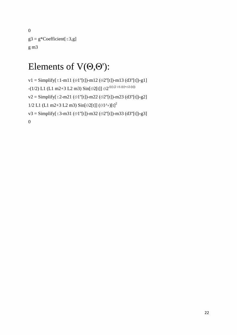
g3 = g*Coefficient[3,g]
g m3
Elements of V(,'):
v1 = Simplify[1-m11 (1''[t])-m12 (2''[t])-m13 (d3''[t])-g1]
-(1/2) L1 (L1 m2+3 L2 m3) Sin[2[t]] 2[t] (2 1[t]+2[t])
v2 = Simplify[2-m21 (1''[t])-m22 (2''[t])-m23 (d3''[t])-g2]
1/2 L1 (L1 m2+3 L2 m3) Sin[2[t]] (1^)[t]2
v3 = Simplify[3-m31 (1''[t])-m32 (2''[t])-m33 (d3''[t])-g3]
0