KINEMATIC AND DYNAMIC BEHAVIOR OF ARTICULATED … · KINEMATIC AND DYNAMIC BEHAVIOR OF ARTICULATED...

KINEMATIC AND DYNAMIC BEHAVIOR OF ARTICULATED ROBOT

MANIPULATORS BY TWO BARS

Felipe Costa Cardoso, [email protected]

Tobias Anderson Guimarâes, [email protected]

Renato de Sousa Dâmaso, [email protected]

Emerson de Sousa Costa, [email protected]

Federal Center of Technological Education of Minas Gerais

Álvares de Azevedo street, 400, Bela Vista, Divinópolis – MG, Brazil

Abstract. The manipulators coming evolving a lot lately, thanks to this increasingly competitive market that requires

the demand for a production line, in addition to automated, with high accuracy of movement. In this context, the

purpose of this study is to examine the influence of kinematics and dynamics of articulated manipulators of two bars on

the accuracy of their trajectory. Particularly, the forces of inertia caused by the Coriolis acceleration are usually not

taken into account, nor even the mathematical modeling and the dimensioning of actuators of industrial robots. Thus, it

might cause positioning errors and errors in the trajectory of the effector of the manipulator. This work will undertake

a study on the early component of acceleration. To attain the goal of this work one manipulator articulated by two bars

will have its kinematics and dynamics modeled. Since, from this model, there will be an analysis of possible errors in

the trajectory of the manipulator, caused by the Coriolis acceleration. The results presented here open a discussion

about the influence of the Coriolis acceleration in the trajectory of an industrial manipulator. This can be worked out

further in future work.

Keywords: Kinematics. Mathematical Modeling. Coriolis acceleration.

1. INTRODUCTION

The Industrial manipulators coming evolving a lot lately. They are no longer just in the manufacturing

industry, carrying pieces of one side to another. Now also perform welding in automobile production lines, are present

in industries of electronics (such as electronic boards) and are being used even in medical fields. That is, these robots,

currently, must be more precise than before.

The accuracy of movements to be performed on the trajectory of robot manipulators is the key performance

requirements that must be taken into account. Thus, the industrial automation assumes role of paramount importance,

since it allows to perform operations in less time and with higher quality.

As today's automation is present in virtually all large companies, the difference is this can offer the quality and

reliability of its products. Since to increase these characteristic, should increase the accuracy of the manipulators who

produce it. For example, manipulators that perform welding on a production line for an automotive manufacturer cannot

introduce any inaccuracy. A poorly solder made commits the entire structure of the automobile. Therefore, this paper

will study and analyze a manipulator who interferes in its accuracy.

This idea of robotics has been devised by men since the mid-fifteenth century. The first to contribute to this

idealization was the great Leonardo da Vinci. This genius was the creator of the first robot with a human form. This

robot was able to settle down and get up, lift up your arms and turn your neck. Furthermore, and even more fascinating,

Leonardo also has the authority to create the first programmable robot in history. This consisted in a kind of cart, which

had the ability to ride and corner alone and programmable way (Leonardo-da-vinci-biography.com©).

After Leonardo robotics has continued to evolve. In the eighteenth century dolls with movements staged

theatrical. His control was very rude, the movements were made from wires and pulleys. And so the evolution was

followed until in 1954, when was registered the first patent for an industrial robot automatic. Since then, the way that

men saw the robots was changing. Robots no longer have humanoid forms without specific tasks, taking on an idea of

automating repetitive tasks, thus becoming major allies of industries.

Over time, these robots were seen as a great opportunity to modernize, increase flexibility and competitiveness

for the industries. Now they seem more like a kind of machinery for use in industries, helping the man in the production

process. Thus, especially in more competitive sectors of the industries in developed countries, the production lines were

being flooded by robots that automate them. Workers no longer had to perform repetitive work or so that put their

health or life at risk.

With advances in technology, these manipulators are becoming increasingly advanced, complex and

comprehensive. Thus, it is increasingly difficult to define a manipulator as comprehensive manner. According

BARRIETOS (1997), an industrial robot is a reprogrammable multifunctional manipulator that can move materials,

parts, tools or special devices in varying trajectories and programmed to perform different tasks.

ABCM Symposium Series in Mechatronics - Vol. 5 Copyright © 2012 by ABCM

Section VII - Robotics 132

Currently, there are various types and categories of robots. They can be used in many, if not all, areas of man's

work. Industrial manipulators are evolved in such a way that no longer only in the manufacturing industry, carrying

pieces of one side to another. Now they are used even in medical areas. That is, these robots have to be much more

accurate today, which needed some time ago.

It is in this context that this work fits. As a characteristic that is increasingly being improved and refined in

industrial manipulators is the positioning accuracy, this paper seeks to study the kinematics and dynamics of an

industrial manipulator to better understand what characteristics influence this aspect of these robots.

To accomplish this, an articulated manipulator by two bars is modeled, first in a static way and then

dynamically.

This work is organized in the following structure: first there will be the static modeling of the manipulator,

then the dynamic modeling and finally, the analysis of results.

2. STATIC ANALYSIS OF MANIPULATOR

The first part of the industrial manipulator to be contemplated is the static. Thus, a simulation was conducted to

get up the static stability of manipulator. That is, the intent is to verify how much torque it takes to keep one robotic arm

of three bars in static balance and which angle this torque happens. Is verified also in which angles the static of the

manipulator becomes easier or more difficult, and how much force or torque is required to maintain this balance.

This analysis will be made to eventually be able to have the concept of the influence or not of the Coriolis

acceleration in the trajectory of an industrial manipulator. This present analysis, along with others held forth, will be

used to arrive at such a notion.

For this check on the static manipulator could be accomplished, we developed a routine called

"analise_estatica" in MATLAB®. In this routine a generic robotic arm is created. You can characterize it as needed,

passing as parameters the length of the bars and their respective weights, and the payload that this will rise.

In order to demonstrate what this routine does, then it is an example where a robotic arm with 0.30 m size bars

of 1 N mass with payload of 0.5 N is created.

>> analise_estatica(1,1,1,0.50,0.30,0.30,0.30)

Running this example we get how out of the system the following data:

Maximum torque at the first bar =

1.8000

It happens to an angle theta (the first joint angle) of =

0

Max Torque second bar =

0.9000

It happens with an alpha angle (angle of the second joint) of =

0

Max Torque third bar =

0.3000

It happens with a range angle (angle of the third joint) of =

0

Making an initial analysis of these results, we arrive at a preliminary conclusion that the maximum torque

always happen when the bar is at an angle of zero degree with respect to a horizontal reference. Another conclusion is

that the torque is higher in the first joint, followed by the second joint torque, and the smallest one in the third joint.

This happens because the engine of the first joint has to realize a torque that must balance the weight of the three bars

plus the payload, the engine of the second joint must balance the weight of two bars more the payload and finally the

torque on the last joint is smaller, because it only needs to lift the weight of a bar plus the payload.

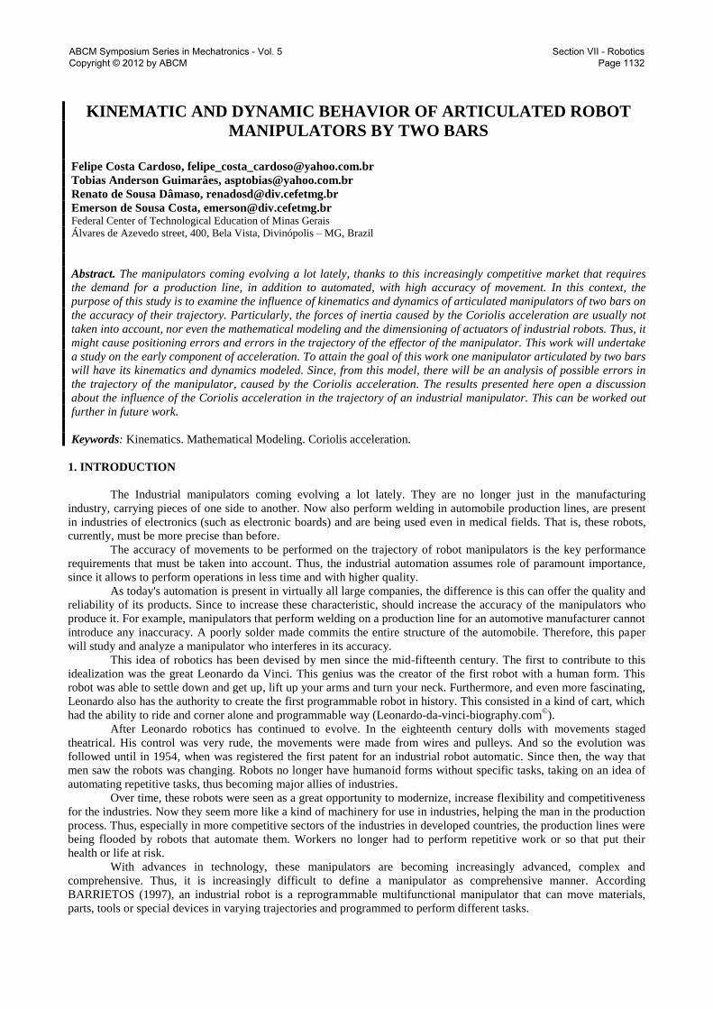
Besides this, the program also generates the three graphs that represent the torque of each joint at certain

angles. In this routine, each arm rotates 360 degrees. But for the computational cost would not be compromised, these

360 degrees were divided into 100 shares, of which the torque needed to maintain the bar static is computed. Thus, for

the first joint, we obtained a surface, as this graph plots the variation of torque in the first bar (bar A) together with the

variation of torque of the second bar (bar B), and the angle theta in which happen these torques. For this plot was

completely represented, i.e., they were shown the torques of the three bars, you would need a chart in four dimensions,

which is not possible. To end this need, especially for this case, the bar C does not move, i.e., does not vary your

movement, being fixed to the bar B. In the chart for the second joint torques are represented in bar two (bar B) and three

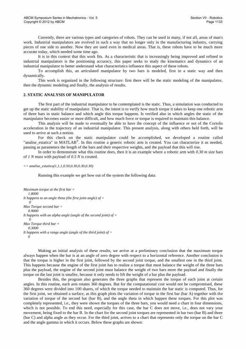
(bar C) and alpha angle as they occur. For the third joint, arrives to a chart that represents only the torque on the bar C

and the angle gamma in which it occurs. Below these graphs are shown:


Section VII - Robotics Page 1133

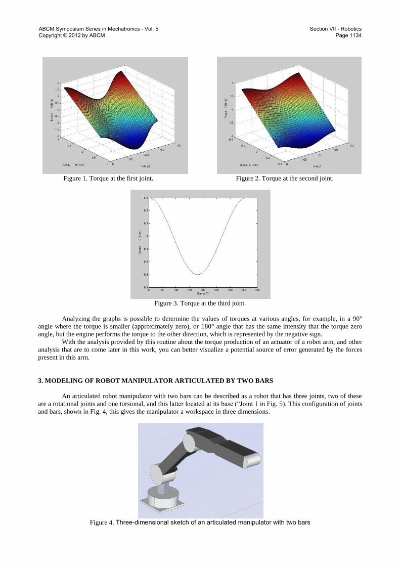
Figure 1. Torque at the first joint. Figure 2. Torque at the second joint.

Figure 3. Torque at the third joint.

Analyzing the graphs is possible to determine the values of torques at various angles, for example, in a 90°

angle where the torque is smaller (approximately zero), or 180° angle that has the same intensity that the torque zero

angle, but the engine performs the torque to the other direction, which is represented by the negative sign.

With the analysis provided by this routine about the torque production of an actuator of a robot arm, and other

analysis that are to come later in this work, you can better visualize a potential source of error generated by the forces

present in this arm.

3. MODELING OF ROBOT MANIPULATOR ARTICULATED BY TWO BARS

An articulated robot manipulator with two bars can be described as a robot that has three joints, two of these

are a rotational joints and one torsional, and this latter located at its base (“Joint 1 in Fig. 5). This configuration of joints

and bars, shown in Fig. 4, this gives the manipulator a workspace in three dimensions.

Figure 4. Three-dimensional sketch of an articulated manipulator with two bars



Will be present two forms of direct modeling for this manipulator. The first is using the Denavit-Hartenberg

notation and the second is the geometric method.

3.1. Modeling the direct kinematics for Denavit-Hartenberg

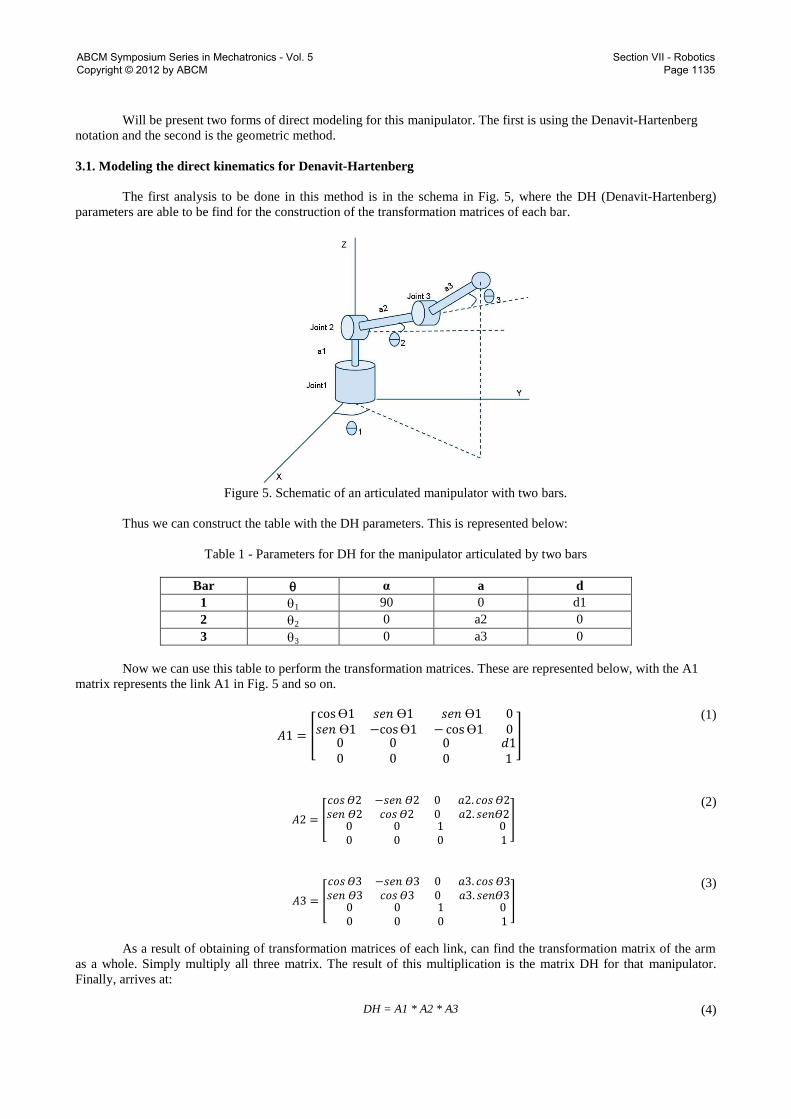
The first analysis to be done in this method is in the schema in Fig. 5, where the DH (Denavit-Hartenberg)

parameters are able to be find for the construction of the transformation matrices of each bar.

Figure 5. Schematic of an articulated manipulator with two bars.

Thus we can construct the table with the DH parameters. This is represented below:

Table 1 - Parameters for DH for the manipulator articulated by two bars

Bar α a d

1 1 90 0 d1

2 2 0 a2 0

3 3 0 a3 0

Now we can use this table to perform the transformation matrices. These are represented below, with the A1

matrix represents the link A1 in Fig. 5 and so on.

(1)

(2)

(3)

As a result of obtaining of transformation matrices of each link, can find the transformation matrix of the arm

as a whole. Simply multiply all three matrix. The result of this multiplication is the matrix DH for that manipulator.

Finally, arrives at:

DH = A1 * A2 * A3 (4)



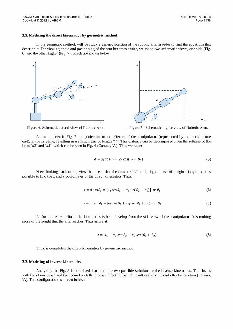
3.2. Modeling the direct kinematics by geometric method

In the geometric method, will be study a generic position of the robotic arm in order to find the equations that

describe it. For viewing angle and positioning of the arm becomes easier, we made two schematic views, one side (Fig.

6) and the other higher (Fig. 7), which are shown below:

Figure 6. Schematic lateral view of Robotic Arm. Figure 7. Schematic higher view of Robotic Arm.

As can be seen in Fig. 7, the projection of the effector of the manipulator, (represented by the circle at one

end), in the xy plane, resulting in a straight line of length “d”. This distance can be decomposed from the settings of the

links „a2‟ and „a3‟, which can be seen in Fig. 6 (Carrara, V.). Thus we have:

(5)

Now, looking back to top view, it is seen that the distance “d” is the hypotenuse of a right triangle, so it is

possible to find the x and y coordinates of the direct kinematics. Thus:

(6)

(7)

As for the “z” coordinate the kinematics is been develop from the side view of the manipulator. It is nothing

more of the height that the arm reaches. Thus arrive at:

(8)

Thus, is completed the direct kinematics by geometric method.

3.3. Modeling of inverse kinematics

Analyzing the Fig. 8 is perceived that there are two possible solutions to the inverse kinematics. The first is

with the elbow down and the second with the elbow up, both of which result in the same end effector position (Carrara,

V.). This configuration is shown below:



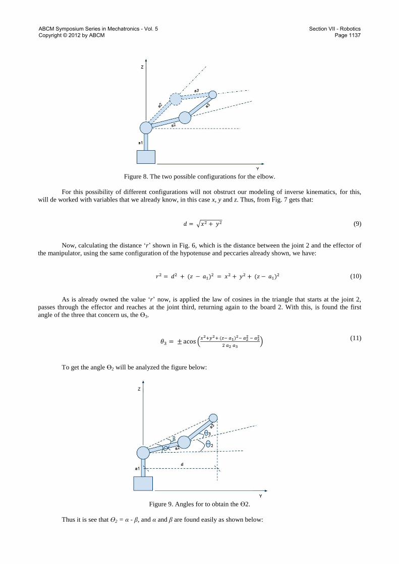
Figure 8. The two possible configurations for the elbow.

For this possibility of different configurations will not obstruct our modeling of inverse kinematics, for this,

will de worked with variables that we already know, in this case x, y and z. Thus, from Fig. 7 gets that:

(9)

Now, calculating the distance „r‟ shown in Fig. 6, which is the distance between the joint 2 and the effector of

the manipulator, using the same configuration of the hypotenuse and peccaries already shown, we have:

(10)

As is already owned the value „r‟ now, is applied the law of cosines in the triangle that starts at the joint 2,

passes through the effector and reaches at the joint third, returning again to the board 2. With this, is found the first

angle of the three that concern us, the 3.

(11)

To get the angle 2 will be analyzed the figure below:

Figure 9. Angles for to obtain the 2.

Thus it is see that ϴ2 = α - β, and α and β are found easily as shown below:



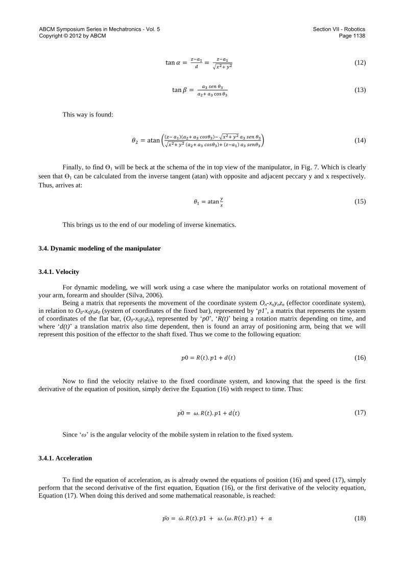
(12)

(13)

This way is found:

(14)

Finally, to find 1 will be beck at the schema of the in top view of the manipulator, in Fig. 7. Which is clearly

seen that 1 can be calculated from the inverse tangent (atan) with opposite and adjacent peccary y and x respectively.

Thus, arrives at:

(15)

This brings us to the end of our modeling of inverse kinematics.

3.4. Dynamic modeling of the manipulator

3.4.1. Velocity

For dynamic modeling, we will work using a case where the manipulator works on rotational movement of

your arm, forearm and shoulder (Silva, 2006).

Being a matrix that represents the movement of the coordinate system On-xnynzn (effector coordinate system),

in relation to O0-x0y0z0 (system of coordinates of the fixed bar), represented by „p1‟, a matrix that represents the system

of coordinates of the flat bar, (O0-x0y0z0), represented by „p0‟, „R(t)‟ being a rotation matrix depending on time, and

where „d(t)‟ a translation matrix also time dependent, then is found an array of positioning arm, being that we will

represent this position of the effector to the shaft fixed. Thus we come to the following equation:

(16)

Now to find the velocity relative to the fixed coordinate system, and knowing that the speed is the first

derivative of the equation of position, simply derive the Equation (16) with respect to time. Thus:

(17)

Since „ω‟ is the angular velocity of the mobile system in relation to the fixed system.

3.4.1. Acceleration

To find the equation of acceleration, as is already owned the equations of position (16) and speed (17), simply

perform that the second derivative of the first equation, Equation (16), or the first derivative of the velocity equation,

Equation (17). When doing this derived and some mathematical reasonable, is reached:

(18)



Since „a‟ is the linear acceleration of the arm, the term “ ” is called “transverse acceleration” and the

last term “ ” is the centripetal acceleration caused by rotation of the handle (SILVA, 2006).

If the effector of this manipulator, that is, the vector p1, which represents it, is varying with respect to the

mobile system, there is the appearance of another term in Equation (18). This term is a representation of a physical

force called the “Coriolis acceleration”. This acceleration can be explained as follows: if is being in an inertial frame,

i.e., a frame in which the acceleration is zero, and is observed an accelerated motion, such as a robotic arm, initially

static, entering in a rotation on its own axis, the moment that begins the movement the tendency of the tip of the

manipulator stay inert is may be explained by Newton‟s First Law, or Law of Inertia. So, in this case, the twist in the

arm caused by this tendency of the effector to get static and because there is acceleration at its base, is explained by

Newton‟s laws.

But if where a non-inertial reference, where the acceleration is not zero, Newton‟s laws no longer are used.

This is where the Coriolis acceleration enters. If, somehow, were possible be on the robotic arm mentioned above, and

be repeated his range of motion, then it would be in a non-inertial reference. Thus the explanation for the twist of the

handle would be the Coriolis acceleration. This acceleration tends to divert the movement of the arm laterally, and

therefore it is not taken into consideration in moving the manipulator, could become a source of error.

So, back to the acceleration equation, including the Coriolis acceleration whose equation is:

(19)

Where „ω’ is the angular velocity and „v‟ is the velocity of the body measured by the no inertial observer.

Porting our equation for the acceleration of the manipulator will be as follows:

(20)

In this case:

(21)

Thus replacing (21) in (22) is obtained

(22)

Thus, as will be shown later, when it is taken into account the Coriolis acceleration, the physical forces present

in this robotic arm will be higher than when this is not taken into account. In the “Conclusions” a deeper analysis of

what can happen in this manipulator will be performed.

4. ANALISYS OF THE RESULTS

After have been modeled the primary characteristics of an industrial manipulator articulated by two bars, will

be held one of the sources of errors that might interfere in its trajectory. This analysis is modeled by the equations for

the acceleration of the manipulator and simple physical formulations in the case, the formula of force, and is taken into

account all the modeling done for the manipulator, for example, made to its torque.

This analysis is done with the intention of initiating an investigation of where and when the Coriolis

acceleration will interfere in the trajectory of an industrial robot. Not planning to make a closed analysis of its effects.

Thus, we set out some calculations on these possible interferences in the arm movements. These are shown below.

Consider a force (F) present in the effector of a manipulator in motion as:

(23)

Where, „m‟ is mass of the manipulator in motion (weight of the robotic arm over the payload), and „a‟ the

acceleration on this manipulator.

As seen in the subsection dealing with modeling of acceleration, if it has not taken into account the Coriolis

acceleration then is obtained an acceleration equal to:

(24)

So the formula for the force present in the manipulator will be:



(25)

However, if modeling has taken into account the Coriolis acceleration will be another, different from that

shown in Equation (24), which as noted earlier, is:

(26)

And thus get another force present in our manipulator. This is shown below:

(27)

If analyzing the Equations (25) and (27) for the force acting on the manipulator in motion, is clearly seen that

when is take into account the Coriolis acceleration the force acting on the arm gets another component and becomes

larger.

At this time of the analysis, one should reflect the extent to which this force may be causing interference in the

trajectory of the manipulator. The first reflection that arises is that for small accelerations of robot arms, this new

component generated by Coriolis can be neglected without much damage to the control of the manipulator. As for

robots working at very high speeds and accelerations that the Coriolis acceleration is already present and might interfere

in the motion and control arm.

Exemplifying, one can think of the work that the controller of the manipulator arm will have to put in a correct

trajectory. Thanks to the feedback that every manipulator has your controller knows where and when the effector is in a

certain position, albeit with some delay. So if this driver is working with high accelerations he must compensate the

Coriolis acceleration, which thanks to the inertia of the arm will extend the movement beyond the expected. Roughly,

one can get an idea of this in the following calculations.

Being the distance “d” which describes an arm in its trajectory represented by the equation:

(28)

And considering that there was no initial displacement and initial velocity, can simplify the Equation (28) for:

(29)

Thus, performing the same analysis for the force, now with the distance, calculated with and without the

Coriolis acceleration as well is obtained:

Distance without the Coriolis acceleration:

(30)

Showing that equation otherwise:

(31)

Distance with the Coriolis acceleration:

(32)

Showing that equation otherwise:

(33)

That is, is concluded that there is a difference of displacement. More precisely, we have an extra distance of:



(34)

This extra distance represents the difference between positioning the modeling using the Coriolis acceleration

and modeling that has not used. In other words, this distance might interfere in the time that the driver will take to put

the robotic arm in a certain position. For example, if without the Coriolis acceleration it would take three cycles to

correct its closed loop positioning, now with the presence of this, it takes five cycles.

Another reflection that arises is about the torque produced by the actuator arm. As shown in the "Static

Analysis of Manipulator", the engines of the arms are sized so as to satisfy the work that this will hold. But if the design

has been done without taking into account the Coriolis acceleration, and whether this manipulator suffering from the

effects of acceleration, then it may be that when the controller to have the engine perform a torque that he is unable to

exercise it, a glitch occurring in the trajectory of the robot. Or maybe the controller, thanks to the failure of the engine,

gets out of control unable to stabilize the manipulator in a certain position. Being necessary in this case, the replacement

of this engine or the inclusion of a gear box in this joint.

5. CONCLUSION

All this concern with the accuracy of the trajectory of manipulators is generated because the industrial

automation is no longer a novelty in large industries and companies today. Thus, the spread of these ceased to be its

high productivity, since they all already have some degree of automation, and became the standard of quality and value

to your product.

In this context, to study what factors influence the accuracy of the movements of these robots on production

lines, it is a great way to understand them better and get information on how to increase the accuracy and quality of

work provided by them.

We carried out studies on the influence of kinematics and dynamics of articulated manipulators of two bars on

the accuracy of their trajectory. Thus we come to an understanding of how it is their behavior and where there are

possible sources of error.

The forces of inertia caused by the Coriolis acceleration, usually not taken into account, nor even the

mathematical modeling and the dimensioning of actuators of industrial robots, can cause delays and failures of

positioning of the effector of the manipulator.

The intention with the analysis done here, is start a discussion about the influences caused by the Coriolis

acceleration in the trajectory of industrial manipulators. A deeper investigation of the effects of inclusion the Coriolis

acceleration on the behavior of manipulators can be addressed in future work, so that a better understanding of how this

affects acceleration trajectories is formed.

6. REFERENCES

CARRARA, V., “Apostila de Robótica”, Universidade de Braz Cubas, Mogi das Cruzes, Brasil.

CRAIG, JOHN J., “Introductions to Robotics: mechanics and control”, 3º edição, Pearson Prince Hall, 1989.

<http://www.leonardo-da-vinci-biography.com/da-vinci-robotic.html>, Acesso em 17 de janeiro de 2011. ROSÁRIO, J. M., “Princípios de Mecatrônica”, Pearson Prentice Hall, 2005.

SCIAVICCO, L. e SICILIANO, B., “Modeling and Control f Robot Manipulators”, McGraw-Hill Book Company, New

York, USA, 1996

SILVA, M. F. S., “Simulação e programação off-line de robôs de montagem”, Dissertação de Mestrado, Faculdade de

engenharia do porto, Portugal, 1996.

SILVA, R. M., “Introdução à dinâmica e ao controle de manipuladores robóticos”, Apostila do curso de engenharia de

controle e automação, Pontifícia Universidade Católica do Rio Grande do Sul (PUCRS), 2006



http://www.leonardo-da-vinci-biography.com/da-vinci-robotic.html

KINEMATIC AND DYNAMIC BEHAVIOR OF ARTICULATED … · KINEMATIC AND DYNAMIC BEHAVIOR OF ARTICULATED...

Documents

Transcript of KINEMATIC AND DYNAMIC BEHAVIOR OF ARTICULATED … · KINEMATIC AND DYNAMIC BEHAVIOR OF ARTICULATED...