Ke y n e sai n ec o n o mci s wti h o u t t h e Lm is c ...
25
KEYNESIAN ECONOMICS WITHOUT THE LM AND IS CURVES: A DYNAMIC GENERALIZATION OF THE TAYLOR- ROMER MODEL EVAN F. KOENIG RESEARCH DEPARTMENT WORKING PAPER 0813 Federal Reserve Bank of Dallas
Transcript of Ke y n e sai n ec o n o mci s wti h o u t t h e Lm is c ...

Keynesian economics without the Lm and is curves: a dynamic GeneraLization of the tayLor-
romer modeL
Evan F. KoEnig
research department worKinG paper 0813
Federal Reserve Bank of Dallas
Keynesian Economics without the LM and IS Curves:
A Dynamic Generalization of the Taylor-Romer Model
by
Evan F. Koenig
Adjunct Professor of Economics
Southern Methodist University
Vice President and Senior Policy Advisor
Federal Reserve Bank of Dallas
2200 N. Pearl Street
Dallas, TX 75201
September 2008
Keynesian Economics without the LM and IS Curves:
A Dynamic Generalization of the Taylor-Romer Model
Abstract: John Taylor and David Romer champion an approach to teaching undergraduate
macroeconomics that dispenses with the LM half of the IS-LM model and replaces it with a rule
for setting the interest rate as a function of inflation and the output gap–i.e., a Taylor rule. But
the IS curve is problematic, too. It is consistent with the permanent-income hypothesis only when
the interest rate that enters the IS equation is a long-term rate–not the short-term rate controlled
by the monetary authority. This article shows how the Taylor-Romer framework can be readily
modified to eliminate this maturity mis-match. The modified model is a dynamic system in output
and inflation, with a unique stable path that behaves very much like Taylor and Romer’s aggregate
demand (AD) schedule. Many–but not all–of the original Taylor-Romer model’s predictions carry
over to the new framework. It helps bridge the gap between the Taylor-Romer analysis and the
more sophisticated models taught in graduate-level courses.
1
Koenig (1987, 1990, 1993a,b), Kerr and King (1996), and McCallum and Nelson (1999)
propose that the intertemporal maximization condition, or Euler equation, of the representative
household be used in place of the IS curve in IS-LM analysis. This paper makes a similar
substitution within the macroeconomic framework championed by Taylor (2000) and Romer
(2000) as an alternative to the textbook IS-LM model. The Taylor-Romer framework keeps the1
traditional IS and Phillips curves, but dispenses with the LM curve, replacing it with a rule for
setting the short-term real interest rate as a function of inflation and the output gap [Taylor
(1993); Henderson and McKibbin (1993)]. There is nothing wrong with the LM curve, in
principle. However, neither policymakers nor the financial and popular press discuss monetary
policy, these days, except in terms of whether the short-term interest rate is appropriate, given the
state of the economy. Consequently, it is difficult to motivate the study of a model which
assumes that the central bank targets the money supply.2
What’s wrong with the traditional IS curve? The IS equation used by Taylor, Romer, and
most textbooks posits that aggregate demand is decreasing in “the” real interest rate. While its
term is left vague, the fact that the IS curve is combined with an LM curve (in textbook
treatments of the IS-LM model) or with a Taylor rule (in the Taylor-Romer model), means that
the interest rate in the IS equation can only be a short-term rate. This implicit assumption is
difficult to reconcile with modern treatments of the permanent income hypothesis. After all,
standard microeconomic theory says that each household seeks to equate the marginal rate of
substitution between current and future consumption to one plus the real interest rate. Assuming
a constant elasticity of substitution between consumption today and consumption tomorrow, ó,
and a constant pure rate of time preference, ñ, this optimality condition implies that
2
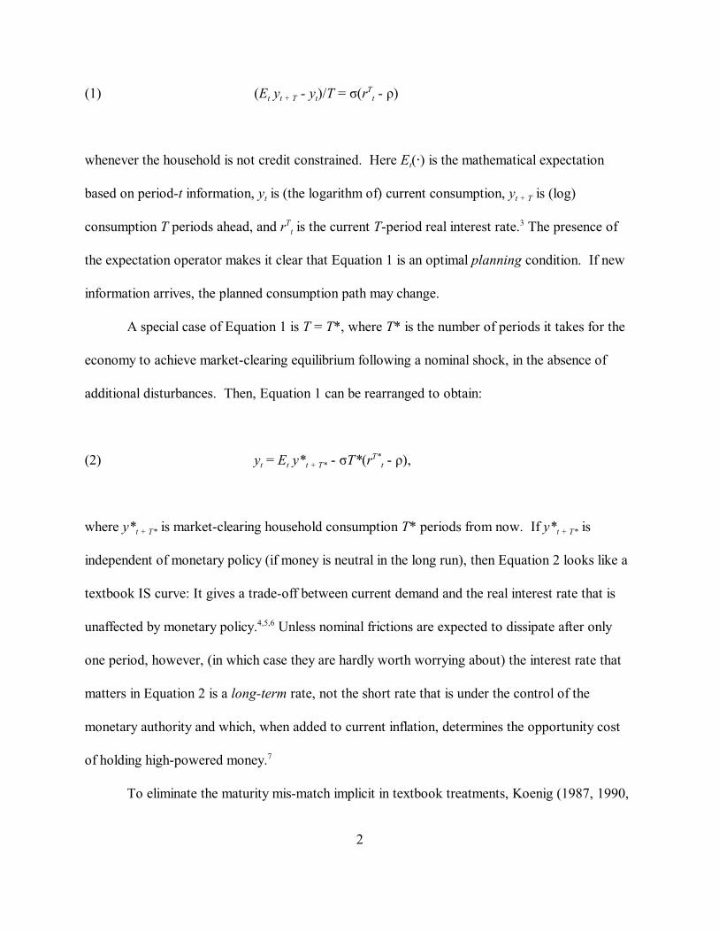
t t + T t t(1) (E y - y )/T = ó(r - ñ)T
twhenever the household is not credit constrained. Here E (�) is the mathematical expectation
t t + Tbased on period-t information, y is (the logarithm of) current consumption, y is (log)
tconsumption T periods ahead, and r is the current T-period real interest rate. The presence ofT 3
the expectation operator makes it clear that Equation 1 is an optimal planning condition. If new
information arrives, the planned consumption path may change.
A special case of Equation 1 is T = T*, where T* is the number of periods it takes for the
economy to achieve market-clearing equilibrium following a nominal shock, in the absence of
additional disturbances. Then, Equation 1 can be rearranged to obtain:
t t t + T* t(2) y = E y* - óT*(r - ñ),T*
t + T* t + T*where y* is market-clearing household consumption T* periods from now. If y* is
independent of monetary policy (if money is neutral in the long run), then Equation 2 looks like a
textbook IS curve: It gives a trade-off between current demand and the real interest rate that is
unaffected by monetary policy. Unless nominal frictions are expected to dissipate after only4,5,6
one period, however, (in which case they are hardly worth worrying about) the interest rate that
matters in Equation 2 is a long-term rate, not the short rate that is under the control of the
monetary authority and which, when added to current inflation, determines the opportunity cost
of holding high-powered money.7
To eliminate the maturity mis-match implicit in textbook treatments, Koenig (1987, 1990,
3
1993a,b), McCallum and Nelson (1999), and Kerr and King (1996) proposed working with the
version of Equation 1 in which T equals 1 rather than T*. The effect is to replace a relationship
between the level of output and the real interest rate with a relationship between expected output
growth and the real interest rate, adding a new, dynamic element to IS-LM analysis. When a
similar substitution is made in the Taylor-Romer framework, it adds a dynamic output-adjustment
equation to the inflation-adjustment equation already in the model.
The additional complexity resulting from the substitution is surprisingly small. The
modified Taylor-Romer model can be analyzed graphically in output–inflation space using a
simple phase diagram. The economy has a unique stable path that looks and behaves much like
Taylor and Romer’s aggregate demand (AD) schedule. Advanced undergraduates and new
graduate students have no trouble manipulating this diagram and tracing the economy’s
adjustment. For some shocks, it’s actually easier to see how the economy’s steady state changes
using the phase diagram than it is using the original Taylor-Romer AD equation.
In broad terms, the modified framework provides a bridge between the Taylor-Romer
analysis and the forward-looking, rational expectations models taught in graduate-level courses.
It reassures students who are familiar with the Taylor-Romer framework that many of its
predictions remain valid in a world where households behave in a manner consistent with
microeconomic theory, and alerts them to circumstances under which the Taylor-Romer
predictions are likely to break down.
4
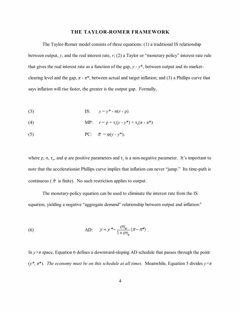
THE TAYLOR-ROMER FRAMEWORK
The Taylor-Romer model consists of three equations: (1) a traditional IS relationship
between output, y, and the real interest rate, r; (2) a Taylor or “monetary policy” interest-rate rule
that gives the real interest rate as a function of the gap, y - y*, between output and its market-
clearing level and the gap, ð - ð*, between actual and target inflation; and (3) a Phillips curve that
says inflation will rise faster, the greater is the output gap. Formally,
(3) IS: y = y* - ó(r - ñ)
y ð(4) MP: r = ñ + ô (y - y*) + ô (ð - ð*)
(5) PC: = ö(y - y*),
ð ywhere ñ, ó, ô , and ö are positive parameters and ô is a non-negative parameter. It’s important to
note that the accelerationist Phillips curve implies that inflation can never “jump.” Its time-path is
continuous ( is finite). No such restriction applies to output.
The monetary-policy equation can be used to eliminate the interest rate from the IS
equation, yielding a negative “aggregate demand” relationship between output and inflation: 8
(6) AD: .
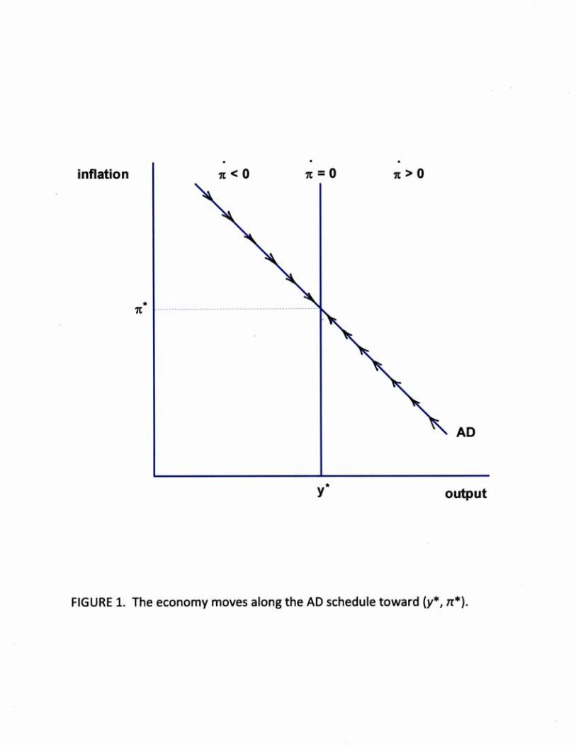
In y×ð space, Equation 6 defines a downward-sloping AD schedule that passes through the point
(y*, ð*). The economy must be on this schedule at all times. Meanwhile, Equation 5 divides y×ð
5
space in half: When y > y*, inflation is rising; and when y < y*, inflation is falling. It follows that
the economy moves up along the AD schedule toward (y*, ð*) whenever y > y*, and moves down
along the AD schedule toward (y*, ð*) whenever y < y*. See Figure 1.9,10
Examples
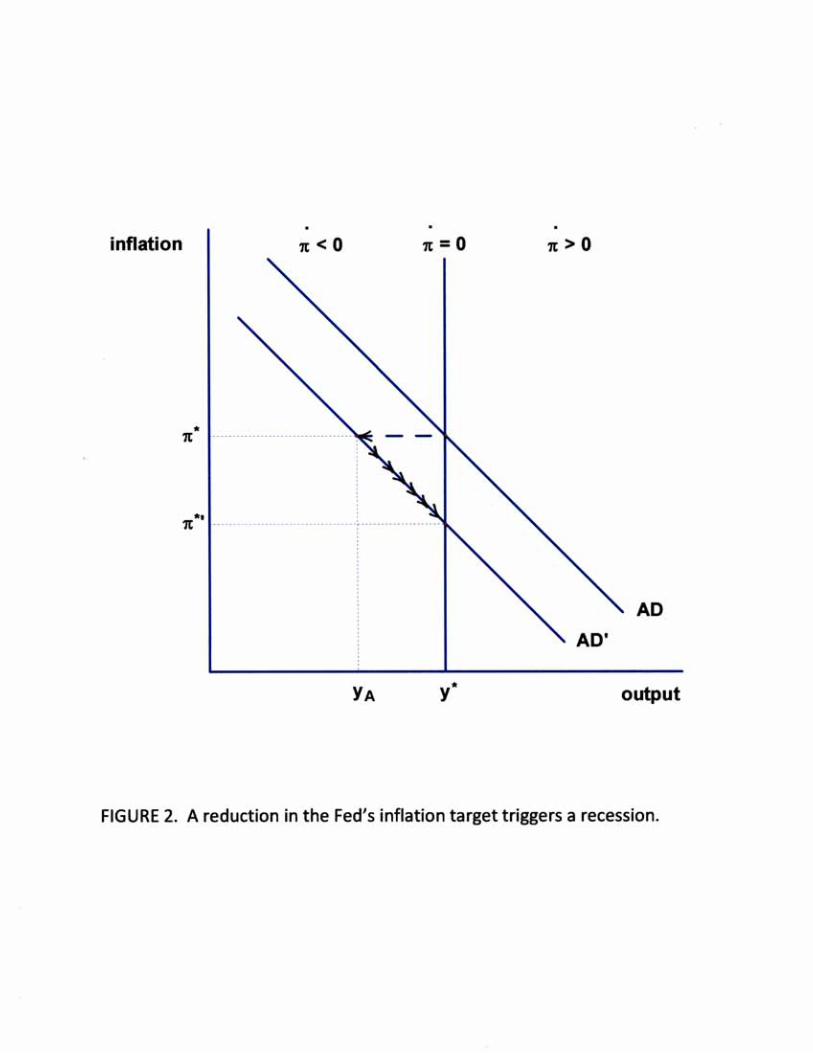
A New Fed Chairman. Suppose that the economy is in steady state, at (y*, ð*), when a Federal
Reserve chairman who wants to lower inflation to ð*' < ð* is confirmed. In Equation 4, ð*'
suddenly replaces ð*. It follows that the AD schedule will shift downward to pass through
(y*, ð*'). Since inflation cannot jump (c.f. Equation 5), it is output that adjusts to put the
Aeconomy on the new AD schedule. Specifically, output instantly drops from y* to y � y* -
ð y A[óô /(1 + óô )](ð* - ð*'). In Figure 2, the economy jumps from (y*, ð*) to (y , ð*). With output
now below potential, inflation gradually declines and, as it does so, the economy moves down the
AD schedule toward (y*, ð*'). The Fed’s more hawkish inflation stance triggers a recession.
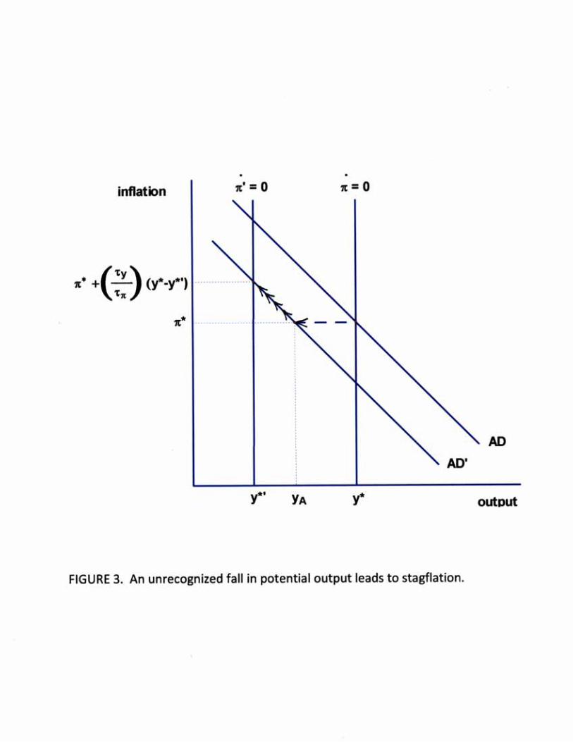
A Fall in Potential Output. Alternatively, suppose that the economy is in steady state, at (y*, ð*),
when potential output suddenly drops to y*' < y*. To make the example more interesting, assume
that the central bank is unaware of the change in potential output and continues to follow the
same policy rule as before. Orphanides (2002 ) argues that something of the sort happened in the
United States during the 1970s. Solving the new IS equation (with y*' in place of y*) and the
unchanged MP equation (with y*, as before) the post-shock AD equation takes the form:
(7) AD': .
6
The implication is that the AD schedule shifts, horizontally, by less than the full drop in potential
output. Intuitively, because the Fed fails to recognize the decline in potential output, it resists
declines in actual output by cutting the interest rate. In the short term, then, output falls from y*
A y y y Ato y � [1/(1 + óô )]y*' + [óô /(1 + óô )]y* rather than to y*'. Because y > y*', there is upward
pressure on the inflation rate, and the economy gradually moves up the new AD schedule.
Following this bout of “stagflation”–declining output accompanied by rising inflation–the
y ðeconomy eventually ends up with output equal to y*' and inflation equal to ð* + (ô /ô )(y* - y*') >
ð* (Figure 3).
Paradoxically, the only way, in Figure 3, for the Fed to eliminate deviations of output from
ypotential is to ignore the output gap when setting policy. Formally, note that if the weight, ô ,
placed on the output gap in the Taylor rule is set equal to zero, then the post-shock aggregate
ðdemand schedule, Equation 7, reduces to: y = y*' - óô (ð - ð*). The AD schedule now shifts,
horizontally, by the full amount of the drop in potential output. The economy moves directly from
its old steady-state equilibrium, (y*, ð*), to a new steady-state equilibrium at (y*', ð*). The
output gap stays at zero and inflation remains constant at its target value.
A DYNAMIC GENERALIZATION OF TAYLOR-ROMER
As noted above, Equation 3–the Taylor-Romer IS schedule–is inconsistent with household
intertemporal utility maximization if r is a short-term interest rate. An alternative specification,
which is consistent with the maximization conditions that students are taught in their intermediate
micro classes, comes from the special case of Equation 1 where T = 1. In continuous time,
Equation 3 is replaced by
7
(3') IS: = ó(r - ñ).
It is understood that Equation 3' may only be violated when new information arrives that is
pertinent to households’ planned spending paths. Output may “jump” coincident with the arrival
of such information.
The monetary-policy and Phillips curve specifications, Equations 4 and 5, are unaltered.11
y ð(4) MP: r = ñ + ô (y - y*) + ô (ð - ð*)
(5) PC: = ö(y - y*).
From Equation 5, inflation rises when y > y* and falls when y < y*, exactly as before. Meanwhile,
Equations 3' and 4 determine the dynamics of output:
y ð(8) = ó[ô (y - y*) + ô (ð - ð*)].
y ðAccording to Equation 8, output rises when ð > ð* - (ô /ô )(y - y*) and falls when ð < ð* -
y ð(ô /ô )(y - y*). In the former case, inflation is so high that the Fed sets the interest rate above the
rate of time preference. Households defer their spending, putting output on a rising path. In the
latter case, inflation is low enough that the Fed sets the interest rate below the rate of time
preference, encouraging households to push their spending forward: Output falls through time.
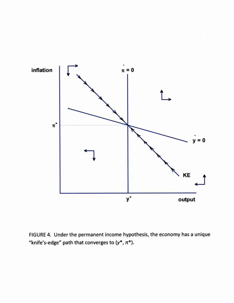
The y×ð plane is now divided into four regions. A vertical line, labeled = 0 in Figure 4,
8
separates regions where inflation is falling from those where inflation is rising. A downward
sloping line, labeled = 0, divides regions where output is rising from regions where output is
falling. The point (y*, ð*) itself is a saddle-point equilibrium: There is a unique, downward-
sloping, “knife’s-edge” path (labeled “KE” in Figure 4) that takes the economy toward (y*, ð*).12
Examples
A New Fed Chairman. Suppose that the economy is initially in steady state at (y*, ð*). If a new,
lower inflation target ( ð*' < ð*) is adopted, nothing happens to the = 0 schedule in the phase
diagram–its position is completely determined by y*–but the = 0 schedule will shift downward
and, along with it, the knife’s-edge path that leads to the economy’s new steady state. The
economy must be on this path when the new monetary policy is implemented. How it gets there
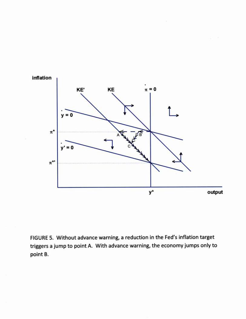
depends on whether the new policy is a surprise or announced in advance.
If a surprise, then the economy behaves very much as it does in the Taylor-Romer model,
with the knife’s edge playing the role of the AD schedule. Households react to the announcement
of the new policy by re-evaluating their spending plans, cutting back on current consumption by
enough to move the economy directly to the new knife’s-edge path (point A in Figure 5). Then,
the economy moves gradually down the knife’s edge to (y*, ð*'), just as it moves down the AD
schedule in the Taylor-Romer model.
If the new inflation target is announced in advance, households have a chance to adjust
their spending plans early, to smooth out their consumption paths. The early adjustment will be
just large enough so that if inflation and spending subsequently evolve according to Equations 5
9
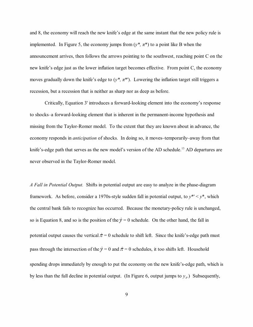
and 8, the economy will reach the new knife’s edge at the same instant that the new policy rule is
implemented. In Figure 5, the economy jumps from (y*, ð*) to a point like B when the
announcement arrives, then follows the arrows pointing to the southwest, reaching point C on the
new knife’s edge just as the lower inflation target becomes effective. From point C, the economy
moves gradually down the knife’s edge to (y*, ð*'). Lowering the inflation target still triggers a
recession, but a recession that is neither as sharp nor as deep as before.
Critically, Equation 3' introduces a forward-looking element into the economy’s response
to shocks–a forward-looking element that is inherent in the permanent-income hypothesis and
missing from the Taylor-Romer model. To the extent that they are known about in advance, the
economy responds in anticipation of shocks. In doing so, it moves–temporarily–away from that
knife’s-edge path that serves as the new model’s version of the AD schedule. AD departures are13
never observed in the Taylor-Romer model.
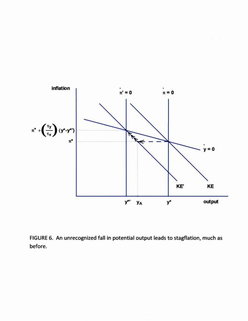
A Fall in Potential Output. Shifts in potential output are easy to analyze in the phase-diagram
framework. As before, consider a 1970s-style sudden fall in potential output, to y*' < y*, which
the central bank fails to recognize has occurred. Because the monetary-policy rule is unchanged,
so is Equation 8, and so is the position of the = 0 schedule. On the other hand, the fall in
potential output causes the vertical = 0 schedule to shift left. Since the knife’s-edge path must
pass through the intersection of the = 0 and = 0 schedules, it too shifts left. Household
spending drops immediately by enough to put the economy on the new knife’s-edge path, which is
Aby less than the full decline in potential output. (In Figure 6, output jumps to y .) Subsequently,
10
the economy moves gradually to the northwest, along the knife’s edge, until y = y*' and ð = ð* +
y ð(ô /ô )(y* - y*').
The nice thing about the phase-diagram apparatus is that it is immediately clear, without
any algebraic manipulations, how the = 0 and = 0 schedules respond to a change in potential
output, and hence how the knife’s-edge path (the surrogate AD schedule) must shift.
The paradox cited earlier continues to hold: When there are imperfectly observed shifts in
potential output, the only way for the monetary authority to eliminate deviations of output from
potential is to completely ignore the output gap when setting policy. In Figure 6, the effect of
ysetting ô = 0 in the policy function is to make the = 0 schedule horizontal. The knife’s-edge
path now shifts leftward by the full decline in potential output, and the economy moves directly
from (y*, ð*) to (y*', ð*).
An Illusory IS Curve
We have seen that there is a negative and monetary-policy-independent relationship
between current spending and the long-term real interest rate (c.f. Equation 2). There is also a
negative and monetary-policy-independent relationship between planned spending growth and the
short-term real interest rate (c.f. Equation 3'). Here, we point out that, much of the time, the data
will give the illusion of an IS-style, negative relationship between the short-term real rate and the
level of current spending. This pseudo-IS relationship arises because there is a close connection
between the level of spending and the growth rate of spending whenever the economy is on the
knife’s-edge path. However, when the economy is off the knife’s edge–i.e., when households

11
learn in advance of a shift in the economic environment–the inverse empirical relationship between
the short-term real interest rate and level of spending will break down. Moreover, the pseudo-IS
relationship is not independent of monetary policy.
Formally, along the knife’s-edge path,
1(9) ð - ð* = (ö/ë )(y - y*),
where
(10)
is the stable root of the differential equation system consisting of Equations 5 and 8. Substituting
back into Equation 8,
y ð 1(11) = ó(ô + ô ö/ë )(y - y*),
along the knife’s-edge path. Finally, combine Equations 3' and 11:
y ð 1(3") y - y* = (r - ñ)/(ô + ô ö/ë ).
y ð 1It is readily verified that (ô + ô ö/ë ) < 0, so that the output gap is negatively related to the real
short-term interest rate provided the economy is traveling along the knife’s edge toward its steady
12
state.
Although Equation 3" has the same form as a traditional IS equation (c.f. Equation 3), it is
subject to the Lucas critique: Output’s sensitivity to interest-rate changes depends on the
y ðcoefficients of the monetary-policy reaction function, ô and ô .
SUMMARY AND CONCLUSIONS
The analysis presented here reinforces the case for using the Taylor-Romer model as the
basic framework for teaching macroeconomics at the principles level. Although the Taylor-
Romer model blurs the distinction between the short-term interest rate that is controlled by the
monetary authority and the long-term rate that theory suggests matters most for household
spending, this shortcoming turns out to be unimportant for tracing the economic effects of
surprise shifts in exogenous variables. Moreover, the maturity mismatch is easily remedied by
replacing the Taylor-Romer IS equation with a household Euler equation, and the Taylor-Romer
AD diagram with a simple phase diagram.
The modified Taylor-Romer model can be used to illustrate how under the permanent
income hypothesis the economy responds in anticipation of policy and other exogenous shifts, to
the extent the shifts become known in advance. The model also nicely illustrates the Lucas
critique: Output and real-interest-rate data may appear to obey a traditional IS relationship, but
with optimizing households this relationship is not reliable and its slope is not independent of the
conduct of monetary policy. In general, the model provides a useful transition between the
principles-level Taylor-Romer analysis and the more sophisticated macro models taught in
graduate-level courses.
13
NOTES
1. See, also, Turner (2006).
2. “False to reality, unconnected with the flow of news, needlessly complex, and leading to
problems in discussing the dynamic evolution of the economy–these four reasons to downplay the
LM curve are not balanced by any offsetting advantages.” – Bradford DeLong (undated)
3. Equation 1 ignores a risk premium, assumes that the real interest rate is known (sensible now
that the Treasury issues inflation-protected securities), and makes use of the approximation
ln(1 + x) � x for small x.
4. Taylor (2000) lists the long-run neutrality of money with respect to real variables as one of
“five key components of modern macroeconomics.”
5. Consistent with the permanent-income hypothesis, current consumption depends on long-run
t t + T*prospects, captured by E y* , but is also affected by the real interest rate. The higher the real
interest rate, the more willing are households to defer consumption–i.e., the steeper is the planned
consumption path.
6. Equation 2 can easily be put into output-gap form:
t t t t + T* t ty - y* = E (y* - y* ) - óT*(r - ñ).T*
Only shocks that affect expected growth in market-clearing output shift this version of the IS
schedule.
7. For an even harsher assessment of the traditional IS curve–and the IS-LM model as a
whole–see King (1993).
8. Romer (2000) shows how to do this using graphs of the IS and MP equations in y×r space.
14
ð9. Key to this convergent behavior is the assumption that ô is greater than zero. If this
condition–the “Taylor principle”–is violated, then the AD schedule is upward rather than
downward sloping, and the economy tends to move away from (y*, ð*), with inflation and output
either both exploding or both imploding.
10. Clearly, the entire analysis could be conducted in terms of the output gap and inflation, rather
than output and inflation. The gap formulation has the advantage that it allows for potential
output to have a trend. Its disadvantage is that it somewhat obscures the implications for output
of a shock to potential output.
11. For simplicity, the analysis in the main text assumes that potential output is expected to
remain constant. Relaxing this assumption requires that the monetary-policy rule be altered,
slightly, to reflect the fact that the flex-price equilibrium real interest rate is increasing in the
economy’s growth rate. In particular, one needs to replace Equation 4 with: r = ñ + (1/ó) +
y ðô (y - y*) + ô (ð - ð*). The phase-diagram analysis in the main text carries through, much as
before, but in (y - y*)×ð space instead of y×ð space.
12. Formally, Equations 5 and 8 form a system of linear differential equations. The roots of this
1 y y ð 2 y y ðsystem are ë = (1/2){óô - [(óô ) + 4öóô ] } and ë = (1/2){óô + [(óô ) + 4öóô ] }. Provided2 1/2 2 1/2
ðthat ô > 0 (the Taylor principle), the first root is negative and the second is positive. The stable
1 1path, or knife’s edge, through (y*, ð*) has the equation ð = ð* + (ö/ë )(y - y*). Recalling that ë
< 0, the stable path is downward sloping. Transversality conditions imply that it is optimal.
13. Suppose that a one-time change in policy (or some other exogenous variable) is announced at
t = 0, to take effect at t = S � 0. The response of the economy must obey the following
principles: (1) At t = 0, households re-evaluate their spending plans in light of the announced
change. Output may jump. (2) For 0 < t � S, the pre-shock Euler conditions continue to apply.
The economy is governed by the original phase diagram. (3) At t = S, the economy must be on
the post-shock knife’s-edge path. The t = 0 output jump is determined by the requirement that
this be so. (4) For t > S, the post-shock dynamics apply, and the economy follows the new
knife’s-edge path toward steady state.
15
References
DeLong, Bradford (undated), www.j-bradford-delong.net/macro_online/interest_rates_ms.html.
Henderson, Dale W. and Warwick J. McKibbin (1993) “A Comparison of Some Basic Monetary
Policy Regimes for Open Economies: Implications of Different degrees of Instrument Adjustment
and Wage Persistence,” Carnegie-Rochester Conference Series on Public Policy 39, (December),
221-317.
Kerr, William and Robert G. King (1996) “Limits on Interest Rate Rules in the IS Model,”
Federal Reserve Bank of Richmond Economic Quarterly 82, (2), 47-75.
King, Robert G. (1993) “Will the New Keynesian Macroeconomics Resurrect the IS-LM Model?”
Journal of Economic Perspectives 7, (1), 67-82.
Koenig, Evan F. (1987) “A Dynamic Optimizing Alternative to Traditional IS-LM Analysis,”
University of Washington Institute for Economic Research Discussion Paper #87-07.
_____ (1990) “Is Increased Price Flexibility Stabilizing? The Role of the Permanent Income
Hypothesis,” Federal Reserve Bank of Dallas Research Paper No. 9011.
_____ (1993a) “Rethinking the IS in IS-LM: Adapting Keynesian Tools to Non-Keynesian
Economies, Part 1” Federal Reserve Bank of Dallas Economic Review, Q3, 33-49.
_____ (1993b) “Rethinking the IS in IS-LM: Adapting Keynesian Tools to Non-Keynesian
Economies, Part 2” Federal Reserve Bank of Dallas Economic Review, Q4, 17-35.
13
McCallum, Bennett T. and Edward Nelson (1999) “An Optimizing IS-LM Specification for
Monetary Policy and Business Cycle Analysis,” Journal of Money, Credit, and Banking 31
(August, Part 1), 296-316.
Orphanides, Athanasios (2002) “Monetary-Policy Rules and the Great Inflation,” American
Economic Review 92, (2), 115-120.
Romer, David (2000) “Keynesian Macroeconomics without the LM Curve,” Journal of Economic
Perspectives 14, (2), 149-169.
Taylor, John B. (1993) “Discretion versus Policy Rules in Practice,” Carnegie-Rochester
Conference Series on Public Policy 39, (December), 195-214.
_____ (2000) “Teaching Modern Macroeconomics at the Principles Level,” American Economic
Review 90, (2), 90-94.
Turner, Paul (2006) “Teaching Undergraduate Macroeconomics with the Taylor-Romer Model,”
International Review of Economic Education 5, (1), 73-82.