Kazuya Akimoto

Piet Mondriaan

Salvador Dalí

Non-parametric non-linear classifiers

Willem MelssenW.Melssen@science.ru.nl

Institute for Molecules and MaterialsAnalytical Chemistry & Chemometrics

www.cac.science.ru.nl

Radboud University Nijmegen

Non-parametric non-linear classifiers

• no assumptions regarding- mean- variance / covariance- normalityof the distribution of the input data

• non-linear relationship between input data and the corresponding output (class membership)

• supervised techniques (input and output based)

Parametric and linear…

LDA

equal (co-)variance

Parametric and linear…

LDA

linear separable classes

…versus non-parametric, non-linear

LDA ???

Some powerful classifiers

• K Nearest Neighbours;

• Artificial Neural Networks;

• Support Vector Machines.

K Nearest Neighbours (KNN)

• non-parametric classifier;(no assumptions regarding normality)

• similarity based;(Euclidean distance, 1 - correlation)

• matching to a set of classified objects.(decision based on consensus criterion)

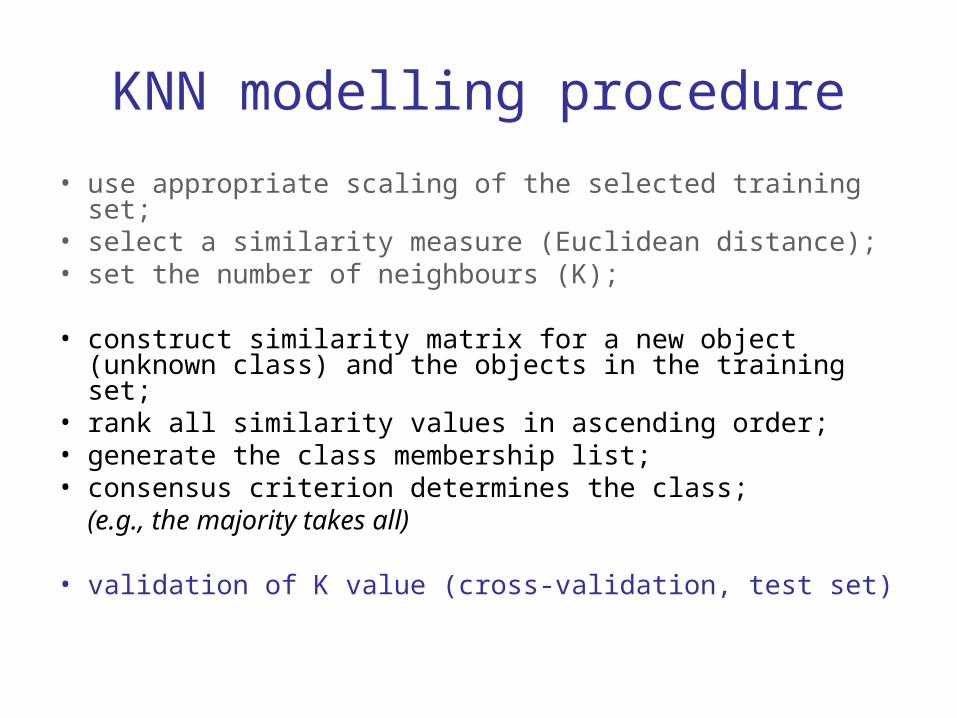
KNN modelling procedure

• use appropriate scaling of the selected training set;• select a similarity measure (Euclidean distance);• set the number of neighbours (K);

• construct similarity matrix for a new object (unknown class) and the objects in the training set;

• rank all similarity values in ascending order;• generate the class membership list; • consensus criterion determines the class;

(e.g., the majority takes all)

• validation of K value (cross-validation, test set)

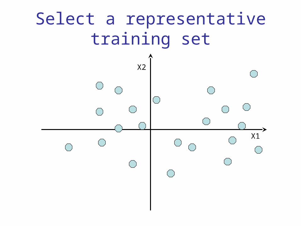
Select a representative training set

X1

X2

Label the data points (supervised)

X1

X2

class A

class B

Classify a new object

X1

X2

class A

class B

One neighbour: K = 1

X1

X2

class A

class B

class B

K = 3

X1

X2

class A

class B

class A

K = 2

X1

X2

class A

class B

class A or B: undecided

K = 11

X1

X2

class A

class B

5 A’s and 6 B’s:confidence?

Classification of brain tumours

• Collaboration with the department of radiology UMCN, Nijmegen; EC project eTumour

• Magnetic resonance imaging

• Voxel-wise in-vivo NMR spectroscopy

• Goal of the project: determination of type and grading of various brain tumours

Magnetic Resonance ImagingT1 weighted T2 weighted

proton density gadolinium

ventricles (CSF)

tumour

grey+white matter

skull

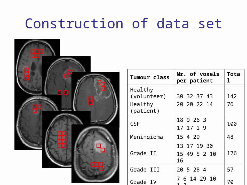
Construction of data set

Tumour classNr. of voxels per patient

Total

Healthy (volunteer)

Healthy (patient)

30 32 37 43

20 20 22 14

142

76

CSF18 9 26 3

17 17 1 9100

Meningioma 15 4 29 48

Grade II13 17 19 30

15 49 5 2 10 16176

Grade III 20 5 28 4 57

Grade IV 7 6 14 29 10 1 3 70

669

MRI combined with MRS

Image variables Quantitated values

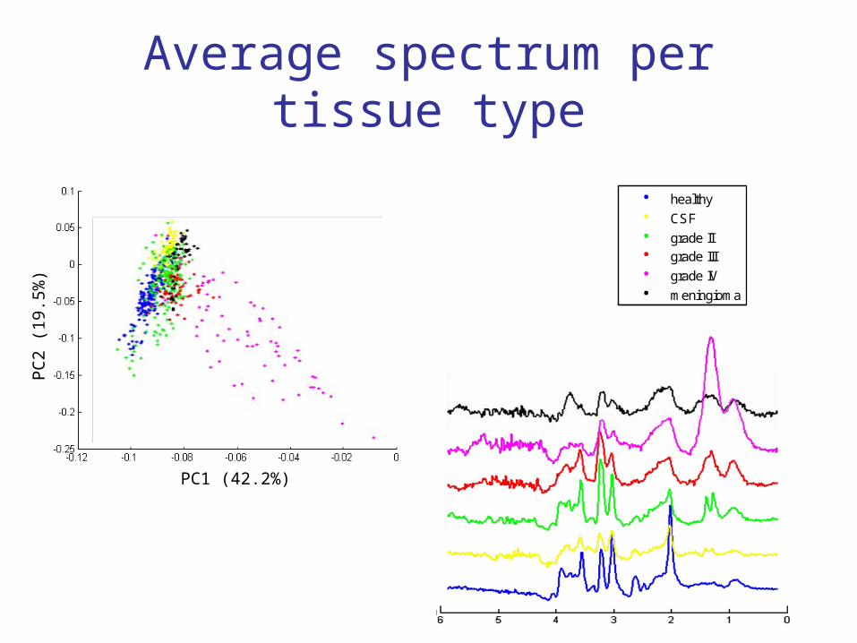
Average spectrum per tissue type

-0.12 -0.1 -0.08 -0.06 -0.04 -0.02 0-0.25

-0.2

-0.15

-0.1

-0.05

0

0.05

0.1

PC1

PC

2

healthy

CSF

grade IIgrade III

grade IV

meningioma

PC1 (42.2%)

PC

2 (1

9.5%

)

Results

10 random divisions of the data in a balanced way

training set (2/3), test set (1/3): 10 different models

• LDA: 90.0% ± 2.0 [87.0 - 92.8] 0.1 sec

• KNN: 95.4% ± 1.0 [92.2 - 97.2] 1.4 sec

Artificial Neural Networks (ANN)

• non-parametric, non-linear, adaptive;

• weights trained by an iterative learning procedure;

ANN architecture

ANN architecture

Neuron or ‘unit’

weighted input(dendrites, synapses)

neuron(soma)

distribution of output(axon)

summation (net) transfer function f(net)

Transfer functions

exponential linear compressive

An easy one: the ‘and’ problem

X1 X2 Y

0 0 0

1 0 0

0 1 0

1 1 1

decision line

Two layer network (perceptron)

sign(x1*w1 + x2*w2 – t) < 0 : class 0

sign(x1*w1 + x2*w2 – t) > 0 : class 1

Hey, this looks like LDA…

Logical ‘exclusive-or’ problem

X1 X2 Y

0 0 0

1 0 1

0 1 1

1 1 0

No single decision line possible…

… but two lines will do

Multi-layer feed-forward ANN

Upper decision line

Lower decision line

Solution

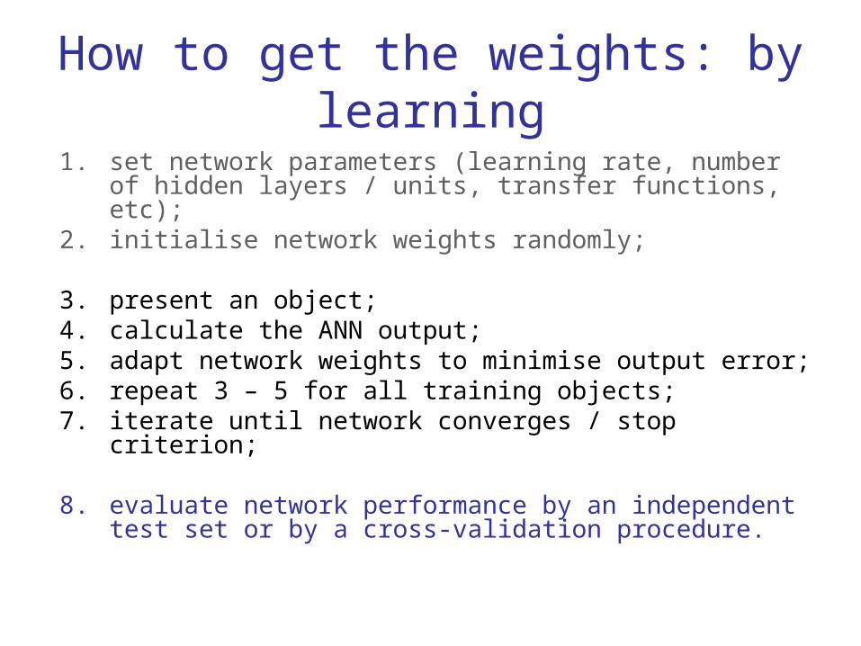
How to get the weights: by learning

1. set network parameters (learning rate, number of hidden layers / units, transfer functions, etc);

2. initialise network weights randomly;

3. present an object;4. calculate the ANN output;5. adapt network weights to minimise output error;6. repeat 3 – 5 for all training objects;7. iterate until network converges / stop criterion;

8. evaluate network performance by an independent test set or by a cross-validation procedure.

Adapting the weights

• adapt weights to minimise the output error E

• weight changes controlled by the learning rate

• error back propagation (from output to input layer)

• Newton-Raphson, Levenberg-Marquardt, etc

local minimum

global minimum

Function of the hidden layer

???

(x, y) points on [0, 1] x [0, 1] grid

specified output for the grid

white: 0black: 1

Output of hidden layer units

unit output for the [0, 1] x [0, 1] grid

Combining linear sub-solutions yields a non-linear classifier…

When to stop training?

Error

Iteration number

training settest set

over-fittingnot converged

External validation set required to estimate the accuracy

Many solutions possible: not unique

Classification of brain tumours

10 random divisions of the data in a balanced way

training set (2/3), test set (1/3): 10 different models

• LDA: 90.0% ± 2.0 [87.0 - 92.8] 0.1 sec

• KNN: 95.4% ± 1.0 [92.2 - 97.2] 1.4 sec

• ANN: 93.2% ± 3.5 [86.4 - 97.7] 316 sec

Support Vector Machines (SVMs)

• kernel-based classifier;

• transforms input space to a high-dimensional feature space;

• exploits Lagrange formalism for the best solution;

• binary (two-class) classifier.

A linear separable problem

X1

X2class B

class A

Goal: to find the optimal separating hyper plane

Optimal hyper plane

X1

X2class B

class A

no objects are allowed between boundaries,

maximisation of distance: unique solution!

Support vectors

bwxxf X1

X2class B

class A

))(( xfsignclass

support vectors

Crossing the borderlines…

X1

X2class B

class A

solution: penalise these objects

Lagrange equation

N

iii

Tp CwwL

1

*

2

1

N

ii

Tiii bxwy

1

N

ii

Tiii bxwy

1

**

N

iiii i

1

**

Target

Constraints

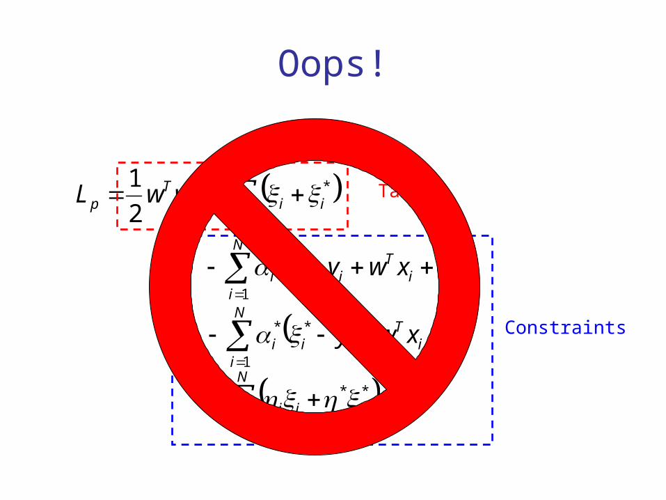
Oops!

N

iii

Tp CwwL

1

*

2

1

N

ii

Tiii bxwy

1

N

ii

Tiii bxwy

1

**

N

iiii i

1

**

Target

Constraints

Minimisation

N

iiii

p xww

L

1

*0

bwxxf bxxN

i

Tiii

1

*

))(( xfsignmembershipclass

only support vectors have a non-zero α

SVM properties

• discriminant function:

• properties:– sparse solution– number of variables irrelevant (dual formalism)– global and unique model– extension to non-linear binary classifier

bxxααxfNSV

iiii

#

1

* ,

A non-linear 2D classification problem

X1

X2class B

class A

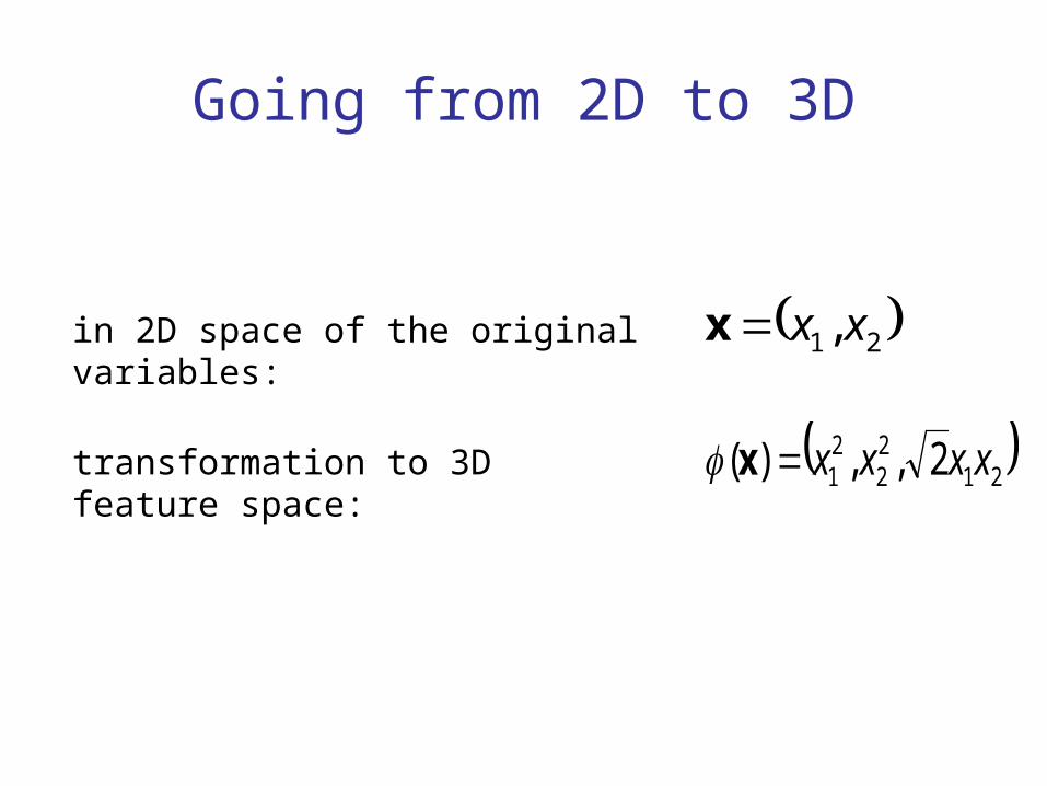
Going from 2D to 3D

2122

21 2,,)( xxxxx

21, xxxin 2D space of the original variables:

transformation to 3D feature space:

Data representation in feature space

2122

21 2,,)( xxxxx

21, xxx

In the feature space the non-linear problem becomes a linear one

From: Belousov et al., Chemometrics and Intelligent Laboratory Systems 64 (2002) 15-25.

2122

21 2,,)( xxxxx

21, xxx

separating plane

Classifiers in feature space

• linear: bxxααxfN

iiii

1

* ,

• a priori: bxxααxfN

iiii

1

* ,

• general: bxxKααxfN

iiii

1

* ,

Kernel

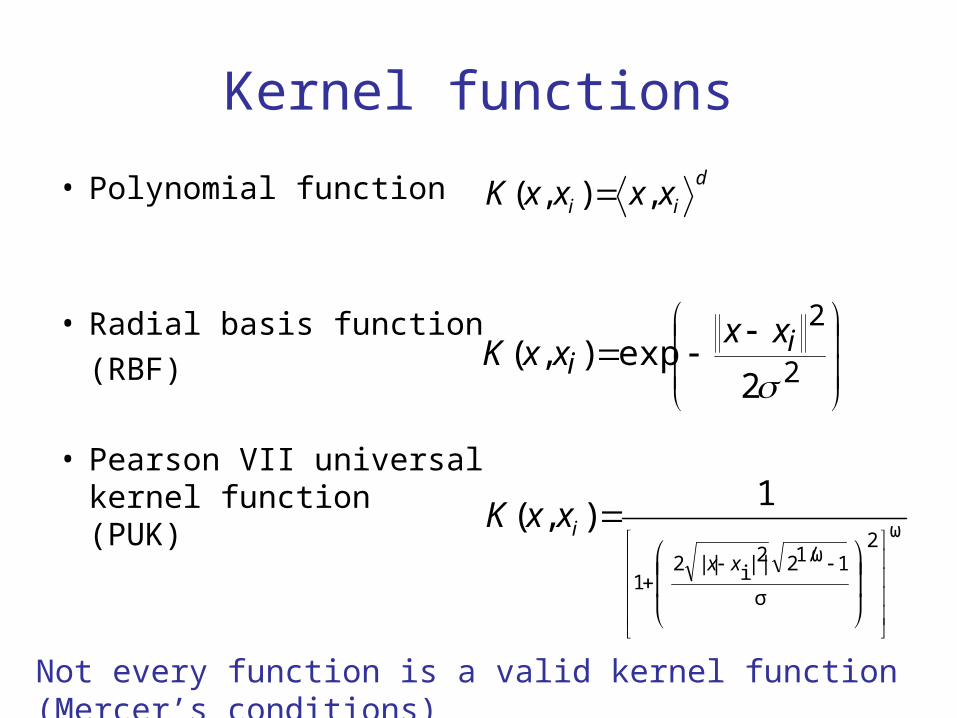
Kernel functions

• Polynomial function

• Radial basis function

(RBF)

• Pearson VII universal kernel function (PUK)

d

ii xxxxK ,),(

2

2

2exp),(

i

ixx

xxK

ω2

σ

11/ω22||i||21

1),(

xx

ixxK

Not every function is a valid kernel function (Mercer’s conditions)

How to construct a SVM model?

1. make a training, test and validation set;

2. set C value (regularisation constant);3. select kernel function and its parameters;4. construct kernel matrix for the training set;5. make SVM model by quadratic programming;6. evaluate performance for the test set;7. repeat steps 2 – 6 (e.g. grid search, GA, Simplex);

8. determine accuracy of best model (validation).

Classification of brain tumours

10 random divisions of the data in a balanced waytraining set (2/3), test set (1/3): 10 different models

• LDA: 90.0% ± 2.0 [87.0 - 92.8] 0.1 sec

• KNN: 95.4% ± 1.0 [92.2 - 97.2] 1.4 sec

• ANN: 93.2% ± 3.5 [86.4 - 97.7] 316 sec

• SVM: 96.9% ± 0.9 [95.8 - 98.6] 8 hours

Best SVM model (98.6%, test)

true / predict H CSF G II G III G IV Men -error (%)

Healthy 70 0 0 0 0 0 0

CSF 0 32 0 0 0 0 0

Grade II 0 0 57 0 0 0 0

Grade III 1 0 0 18 0 0 5

Grade IV 1 0 0 1 21 0 9

Meningioma 0 0 0 0 0 16 0

β-error (%) 3 0 0 5 0 0

SVM is the best one but a bit confused

true / predict H CSF G II G III G IV Men -error (%)

Healthy 70 0 0 0 0 0 0

CSF 0 32 0 0 0 0 0

Grade II 0 0 57 0 0 0 0

Grade III 1 0 0 18 0 0 5

Grade IV 1 0 0 1 21 0 9

Meningioma 0 0 0 0 0 16 0

β-error (%) 3 0 0 5 0 0

Here are the real problems (overlap)

true / predict H CSF G II G III G IV Men -error (%)

Healthy 70 0 0 0 0 0 0

CSF 0 32 0 0 0 0 0

Grade II 0 0 57 0 0 0 0

Grade III 1 0 0 18 0 0 5

Grade IV 1 0 0 1 21 0 9

Meningioma 0 0 0 0 0 16 0

β-error (%) 3 0 0 5 0 0

KNN, ANN and other classifiers

The consumentenbond ratings...KNN ANN SVM

simplicity

uniqueness

performance /

multi-class

outliers

# objects

# variables

speed

Acknowledgements

• Bülent Üstün (SVMs)

• Patrick Krooshof (eTumour examples)