Introduction to R

Linear ModellingAn introduction using R

Karim Malki

19 June 2014

AGENDA• R for statistical analysis

• Understanding Linear Models

• Data pre-processing

• Building Linear Models in R

• Graphing

• Reporting Results

• Further Reading

R For Statistics

R is a powerful statistical program but it is first and foremost a programming language.

Many routines have been written for R by people all over the world and made freely available on the R project website as "packages".

The base installation contains a powerful set of tools for many statistical purposes including linear modelling.

Requires library orMore advanced

Variance and CoVariance

Variance

• Sum of each data point minus the mean for that variable, squared

• When a participant deviates from the mean on one variable, do they deviate on another variable in a similar, or opposite, way? = “Covariance”.

22

1

x Xs

n

Correlationx <- runif(10, 5.0, 15) y <- sample(5:15, 10, replace=T)

xis.atomic(x)str(x)yis.atomic(y)str(y)

var(x)var(y)

cov(x,y)

Correlation

Standardising covariance measures Standardising a covariance value gives a measure of the strength of the relationship -> Correlation coefficient

E.g. covariance divided by (sd of X * sd of Y) is the ‘Pearson product moment correlation coefficient’ This will give coefficients between -1 (perfect negative relationship) and 1 (perfect positive relationship)

cov(x,y)/(sqrt(var(x))*sqrt(var(y)))

myfunction<-function(x,y){cov(x,y)/(sqrt(var(x))*sqrt(var(y)))}

cort(x,y)cor(x,y)

Correlation?faithfuldata(faithful)summary(faithful)dim(faithful)str(faithful)names(faithful)

library(psych)describe(faithful)

> summary (faithful) eruptions waiting Min. :1.600 Min. :43.0 1st Qu.:2.163 1st Qu.:58.0 Median :4.000 Median :76.0 Mean :3.488 Mean :70.9 3rd Qu.:4.454 3rd Qu.:82.0 Max. :5.100 Max. :96.0

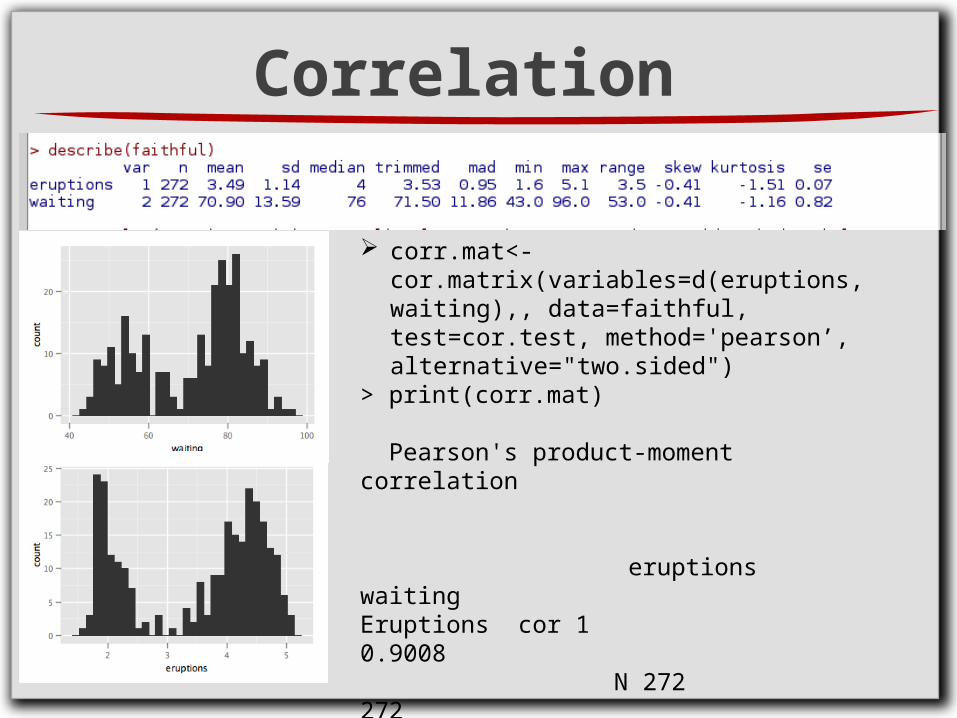
>describe(faithful) var n mean sd median trimmed mad min max range skeweruptions 1 272 3.49 1.14 4 3.53 0.95 1.6 5.1 3.5 -0.41waiting 2 272 70.90 1 3.59 76 71.50 11.86 43.0 96.0 53.0 -0.41 kurtosis seeruptions -1.51 0.07waiting -1.16 0.82>

Correlation

Correlation graphsUse the basic defaults to create a scatter plot of your two variables plot(eruptions~ waiting)

Change the axes titleplot(eruptions, waiting, xlab="X-axis", ylab="Y-axis")

This changes the plotting symbol to a solid circle plot(eruptions, waiting, pch=16)

Adds a line of best fit to your scatter plot abline(lm(waiting ~ eruptions)

The default correlation returns the pearson correlation coefficient cor(eruptions, waiting)

If you specify "spearman" you will get the spearman correlation coefficient

cor(eruptions, waiting, method = "spearman”)

If you use a datset instead of separate variables you will return a matrix of all the pairwise correlation coefficients

cor(dataset, method = "pearson")

Correlationls()hist(faithful$eruptions, col="grey")hist(faithful$waiting, col="grey")attach(faithful)plot(eruptions~waiting)abline(lm(faithful$eruptions~faithful$waiting))

cor(eruptions,waiting)cor(faithful, method = "pearson”)

library(car)scatterplot(eruptions~waiting, reg.line=lm, smooth=TRUE, spread=TRUE, id.method='mahal', id.n = 2, boxplots='xy', span=0.5, data=faithful)

library(psych)cor.test(waiting,eruptions)

Correlation

Correlation

Correlation

corr.mat<-cor.matrix(variables=d(eruptions,waiting),, data=faithful, test=cor.test, method='pearson’, alternative="two.sided")

> print(corr.mat)

Pearson's product-moment correlation

eruptions waiting Eruptions cor 1 0.9008 N 272 272 CI* (0.8757,0.9211) p-value 0.0000

Regression

• Linear Regression is conceptually similar to correlation

• However, correlation does not treat the two variables differently

• In contrast, Linear Regression is asking about the effect of one on the other.

It distinguishes between IVs (the thing that may influence) and DVs (the

things being influenced)

• So, sometimes problematically, you choose which you expect to have the

causal effect

• Fits a straight line that minimises squared error in the DV (vertical distances

of points from the line = “Method of Least Squares”

• And then asks about the relative variance explained by this straight line

model relative to the unexplained variance

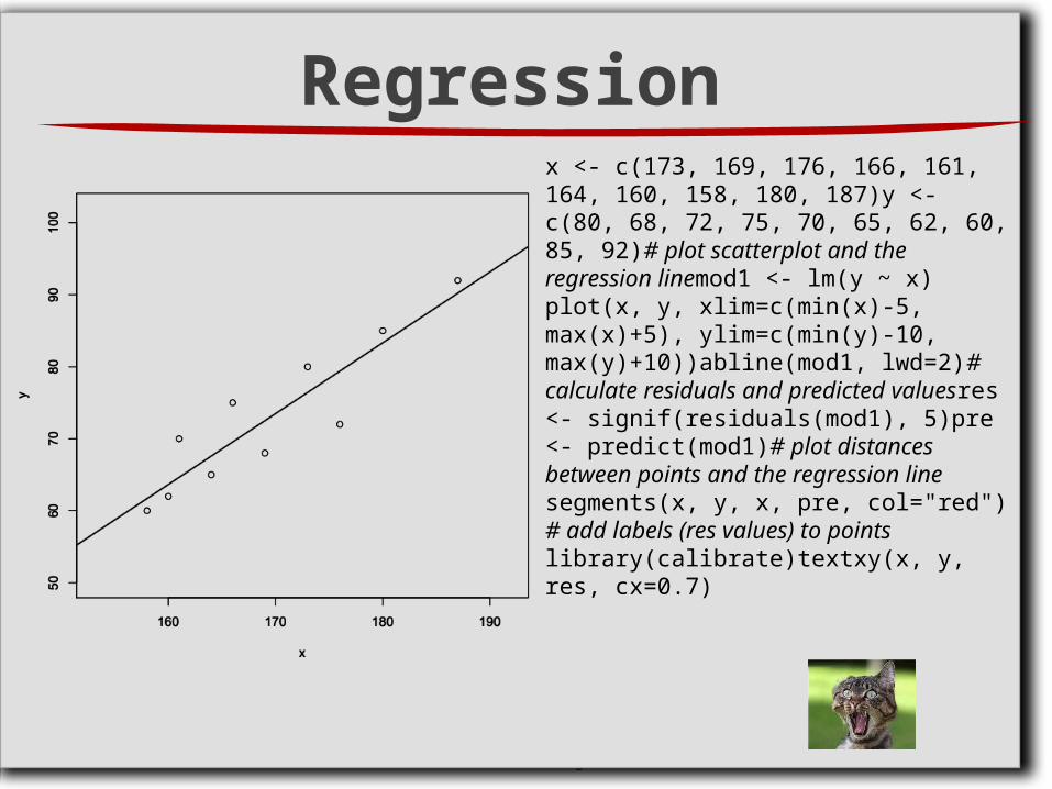
Regressionx <- c(173, 169, 176, 166, 161, 164, 160, 158, 180, 187)y <- c(80, 68, 72, 75, 70, 65, 62, 60, 85, 92)# plot scatterplot and the regression linemod1 <- lm(y ~ x)plot(x, y, xlim=c(min(x)-5, max(x)+5), ylim=c(min(y)-10, max(y)+10))abline(mod1, lwd=2)# calculate residuals and predicted valuesres <- signif(residuals(mod1), 5)pre <- predict(mod1)# plot distances between points and the regression linesegments(x, y, x, pre, col="red")# add labels (res values) to pointslibrary(calibrate)textxy(x, y, res, cx=0.7)

Regression

Method of Least square

Parameters

The regression model know what is the best fitting line but it can tell you only two things. The slope (gradient or coefficient) and the intercept (or constant)

Parameters

Linear Modelling#data(faithful);ls()mod1<- lm(eruptions~waiting,data=faithful)mod1

Coefficients:(Intercept) waiting -1.87402 0.07563

summary(mod1)Call:lm(formula = eruptions ~ waiting, data = faithful)

Residuals: Min 1Q Median 3Q Max -1.29917 -0.37689 0.03508 0.34909 1.19329

Coefficients: Estimate Std. Error t value Pr(>|t|) (Intercept) -1.874016 0.160143 -11.70 <2e-16 ***waiting 0.075628 0.002219 34.09 <2e-16 ***---Signif. codes: 0 ‘***’ 0.001 ‘**’ 0.01 ‘*’ 0.05 ‘.’ 0.1 ‘ ’ 1

Residual standard error: 0.4965 on 270 degrees of freedomMultiple R-squared: 0.8115, Adjusted R-squared: 0.8108 F-statistic: 1162 on 1 and 270 DF, p-value: < 2.2e-16

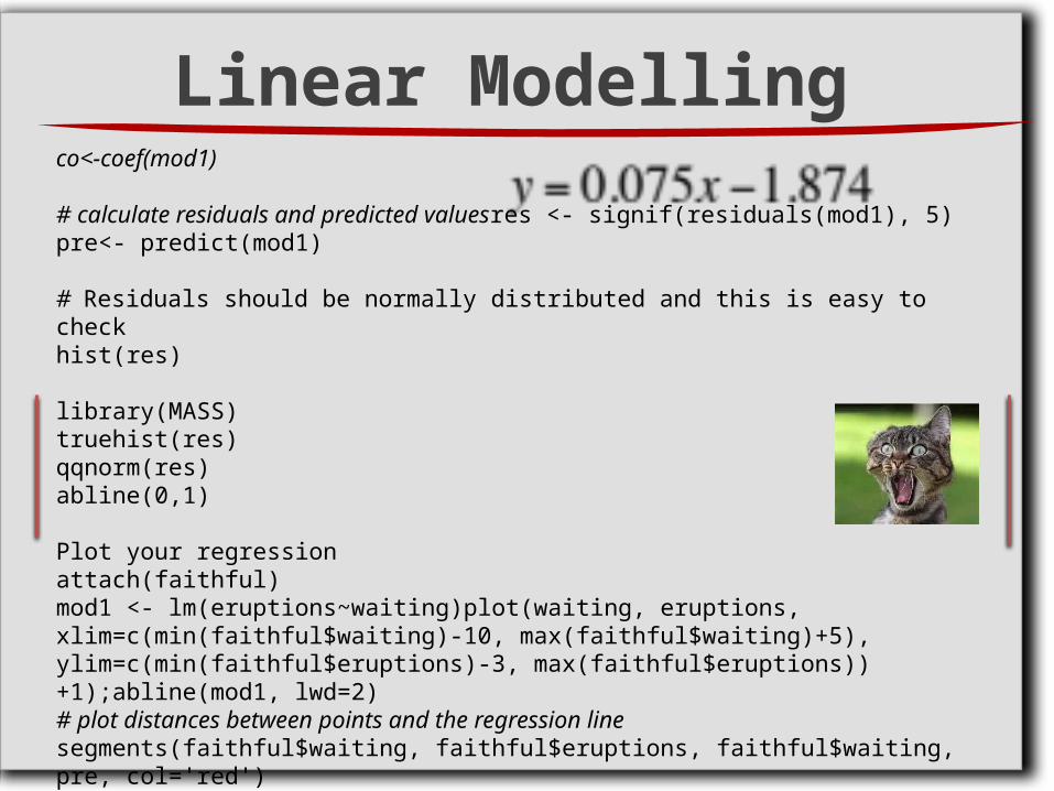
co<-coef(mod1)

# calculate residuals and predicted valuesres <- signif(residuals(mod1), 5)pre<- predict(mod1)

# Residuals should be normally distributed and this is easy to checkhist(res)

library(MASS)truehist(res)qqnorm(res)abline(0,1)

Plot your regressionattach(faithful)mod1 <- lm(eruptions~waiting)plot(waiting, eruptions, xlim=c(min(faithful$waiting)-10, max(faithful$waiting)+5), ylim=c(min(faithful$eruptions)-3, max(faithful$eruptions))+1);abline(mod1, lwd=2)# plot distances between points and the regression linesegments(faithful$waiting, faithful$eruptions, faithful$waiting, pre, col='red')

Linear Modelling

Return p-valuelmp <- function (modelobject) { if (class(modelobject) != "lm") stop("Not an object of class 'lm' ") f <- summary(modelobject)$fstatistic p <- pf(f[1],f[2],f[3],lower.tail=F) attributes(p) <- NULLprint(modelobject) return(p)}

Model FitIf the model does not fit, it may be because of:

Outliers

Unmodelled covariates

Heteroscedasticity (residuals have unequal variance)

Clustering (residuals have lower variance within subgroups)

Autocorrelation (correlation between residuals at successive time points)

Model Fitlibrary(MASS, pysch, lattice, grid, hexbin)library(solaR)data(hills)splom(~hills)

data <- subset(hills, select=c('dist', 'time', 'climb' ))splom(hills, panel=panel.hexbinplot, colramp=BTC, diag.panel = function(x, ...){ yrng <- current.panel.limits()$ylim d <- density(x, na.rm=TRUE) d$y <- with(d, yrng[1] + 0.95 * diff(yrng) * y / max(y) ) panel.lines(d) diag.panel.splom(x, ...) }, lower.panel = function(x, y, ...){ panel.hexbinplot(x, y, ...) panel.loess(x, y, ..., col = 'red') }, pscale=0, varname.cex=0.7 )

Model Fitmod2=lm(time~dist,data=hills)summary(mod2)attach(hills)co2=coef(mod2)plot(dist,time)abline(co2)

fl=fitted(mod2)for(i in 1:35)

lines(c(dist[i],dist[i]),c(time[i],fl[i]),col=‘red’)

#Can you spot outliers?

sr=stdres(mod2)names(sr)truehist(sr,xlim=c(-3,5),h=.4)names(sr)[sr>3]names(sr)[sr<-3]

Model Fitattach(hills)plot(dist,time, ylim=c(0,250))abline(coef(lm1))identify(dist,time, labels=rownames(hills))

What to do with outliersData driven methods for the removal of outliers – some limitations

Fit a better model

Robust regression is an alternative to least squares regression when data are contaminated with outliers or influential observations

Leverage: An observation with an extreme value on a predictor variable is a point with high leverage. Leverage is a measure of how far an independent variable deviates from its mean.

Influence: An observation is influential if removing the observation substantially changes the estimate of the regression coefficients.

Cook's distance (or Cook's D): A measure that combines the information of leverage and residual of the observation.

What to do with outliersattach(hills);summary(ols <- lm(time ~ dist))

opar <- par(mfrow = c(2, 2), oma = c(0, 0, 1.1, 0))plot(ols, las = 1)Influence.measures(lm1)

#Using M estimator

rlm1=rlm(time~dist,data=hills,method=‘MM’)summary(rlm1)

attach(hills)plot(dist,time, ylim=c(0,250))abline(coef(lm1))abline(coef(rlm1),col="red")identify(dist,time)

What to do with outliersattach(hills);summary(ols <- lm(time ~ dist))

opar <- par(mfrow = c(2, 2), oma = c(0, 0, 1.1, 0))plot(ols, las = 1)Influence.measures(lm1)

Using M estimator

rlm1=rlm(time~dist,data=hills,method=‘MM’)summary(rlm1)

attach(hills)plot(dist,time, ylim=c(0,250))abline(coef(lm1))abline(coef(rlm1),col="red")identify(dist,time, labels=rownames(hills))

Linear Modelling

I will be around for questions or, for a slower response, email me:

Karim.malki@kcl.ac.uk