Kapitel 6: Klassifikation - Lehr- und …Model Construction) Classification Introduction 5...
44
DATABASE SYSTEMS GROUP Knowledge Discovery in Databases I: Classification 1 Knowledge Discovery in Databases WiSe 2017/18 Vorlesung: Prof. Dr. Peer Kröger Übungen: Anna Beer, Florian Richter Ludwig-Maximilians-Universität München Institut für Informatik Lehr- und Forschungseinheit für Datenbanksysteme Kapitel 6: Klassifikation
Transcript of Kapitel 6: Klassifikation - Lehr- und …Model Construction) Classification Introduction 5...

DATABASESYSTEMSGROUP
Knowledge Discovery in Databases I: Classification 1
Knowledge Discovery in DatabasesWiSe 2017/18
Vorlesung: Prof. Dr. Peer Kröger
Übungen: Anna Beer, Florian Richter
Ludwig-Maximilians-Universität MünchenInstitut für InformatikLehr- und Forschungseinheit für Datenbanksysteme
Kapitel 6: Klassifikation

DATABASESYSTEMSGROUP
Chapter 5: Classification
1) Introduction
– Classification problem, evaluation of classifiers, numerical prediction
2) Bayesian Classifiers
– Bayes classifier, naive Bayes classifier, applications
3) Linear discriminant functions & SVM1) Linear discriminant functions
2) Support Vector Machines
3) Non-linear spaces and kernel methods
4) Decision Tree Classifiers
– Basic notions, split strategies, overfitting, pruning of decision trees
5) Nearest Neighbor Classifier
– Basic notions, choice of parameters, applications
6) Ensemble Classification
Outline 2

DATABASESYSTEMSGROUP
Additional literature for this chapter
• Christopher M. Bishop: Pattern Recognition and Machine Learning. Springer, Berlin 2006.
Classification Introduction 3

DATABASESYSTEMSGROUP
Introduction: Example
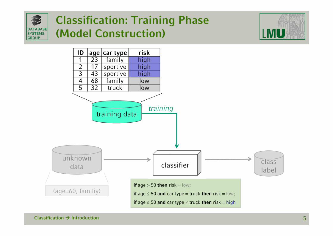
• Training data
• Simple classifierif age > 50 then risk = low;
if age 50 and car type = truck then risk = low;
if age 50 and car type truck then risk = high.
Classification Introduction 4
ID age car type risk1 23 family high2 17 sportive high3 43 sportive high4 68 family low5 32 truck low
DATABASESYSTEMSGROUP
Classification: Training Phase (Model Construction)
Classification Introduction 5
Classifier
(age=60, familiy)if age > 50 then risk = low;
if age 50 and car type = truck then risk = low;
if age 50 and car type truck then risk = high
ID age car type risk1 23 family high2 17 sportive high3 43 sportive high4 68 family low5 32 truck low
training data
classifier
training
unknown data
class label

DATABASESYSTEMSGROUP
Classification: Prediction Phase (Application)
Classification Introduction 6
Classifier
(age=60, family) risk = lowif age > 50 then risk = low;
if age 50 and car type = truck then risk = low;
if age 50 and car type truck then risk = high
training data
classifier
training
unknown data
class label
ID age car type risk1 23 family high2 17 sportive high3 43 sportive high4 68 family low5 32 truck low

DATABASESYSTEMSGROUP
Classification
• The systematic assignment of new observations to known categories according to criteria learned from a training set
• Formally, – a classifier K for a model is a function : → , where
• : data space– Often d-dimensional space with attributes , 1, … , (not necessarily vector space)
– Some other space, e.g. metric space
• 1, … , :set of distinct class labels , 1, … ,• ⊆ : set of training objects, 1, … , , with known class labels ∈
– Classification: application of classifier K on objects from
• Model is the “type” of the classifier, and are the model parameters
• Supervised learning: find/learn optimal parameters for the model from the given training data
Classification Introduction 7
DATABASESYSTEMSGROUP
Supervised vs. Unsupervised Learning
• Unsupervised learning (clustering)
– The class labels of training data are unknown
– Given a set of measurements, observations, etc. with the aim of establishing the existence of classes or clusters in the data
• Classes (=clusters) are to be determined
• Supervised learning (classification)
– Supervision: The training data (observations, measurements, etc.) are accompanied by labels indicating the class of the observations
• Classes are known in advance (a priori)
– New data is classified based on information extracted from the training set
Classification Introduction 8
[WK91] S. M. Weiss and C. A. Kulikowski. Computer Systems that Learn: Classification and Prediction Methods from Statistics, Neural Nets, Machine Learning, and Expert Systems. Morgan Kaufman, 1991.
DATABASESYSTEMSGROUP
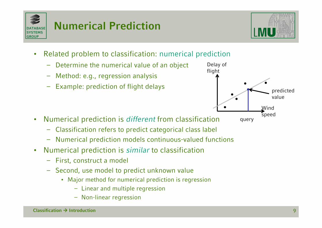
Numerical Prediction
• Related problem to classification: numerical prediction
– Determine the numerical value of an object
– Method: e.g., regression analysis
– Example: prediction of flight delays
• Numerical prediction is different from classification– Classification refers to predict categorical class label
– Numerical prediction models continuous-valued functions
• Numerical prediction is similar to classification– First, construct a model
– Second, use model to predict unknown value• Major method for numerical prediction is regression
– Linear and multiple regression
– Non-linear regression
Classification Introduction 9
Windspeed
Delay offlight
query
predictedvalue
DATABASESYSTEMSGROUP
10
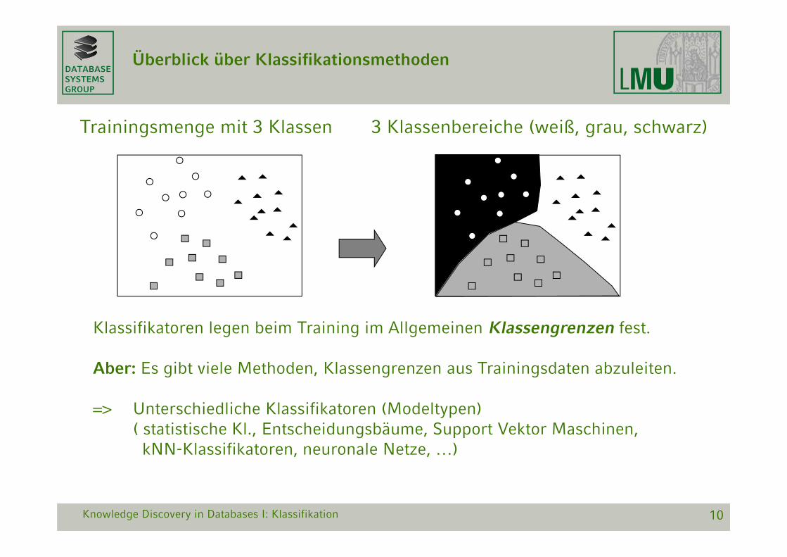
Überblick über Klassifikationsmethoden
Trainingsmenge mit 3 Klassen
Klassifikatoren legen beim Training im Allgemeinen Klassengrenzen fest.
Aber: Es gibt viele Methoden, Klassengrenzen aus Trainingsdaten abzuleiten.
=> Unterschiedliche Klassifikatoren (Modeltypen)( statistische Kl., Entscheidungsbäume, Support Vektor Maschinen,
kNN-Klassifikatoren, neuronale Netze, …)
3 Klassenbereiche (weiß, grau, schwarz)
Knowledge Discovery in Databases I: Klassifikation

DATABASESYSTEMSGROUP
11
Motivation der Klassifikationsmethoden(1)
Bayes Klassifikatoren
NN-Klassifikator
Unterscheidung durch Voronoi-Zellen(1 nächster Nachbar Klassifikator)
Unterscheidung durch Dichtefunktionen.
Klassengrenzen
1-dimensionale Projektion
Knowledge Discovery in Databases I: Klassifikation

DATABASESYSTEMSGROUP
12
Entscheidungsbäume
Support Vektor Maschinen
Motivation der Klassifikationsmethoden(2)
Festlegen der Grenzen durch rekursiveUnterteilung in Einzeldimension.
1
2
33
1
2
44
Grenzen über lineare Separation
Knowledge Discovery in Databases I: Klassifikation

DATABASESYSTEMSGROUP
• Es gibt einen (natürlichen, technischen, sozial-dynamischen, …) Prozess (im statistischen Sinne), der die beobachteten Daten O als Teilmenge der möglichen Daten D erzeugt bzw. für ein x D eine Klassenentscheidung für eine Klasse yi Y trifft.
• Die beobachteten Daten sind Beispiele für die Wirkung des Prozesses.
• Es gibt eine ideale (unbekannte) Funktion, die einen Beispiel-Datensatz auf die zugehörige Klasse abbildet:f: D Y
• Aufgabe des Lernalgorithmus ist es, eine möglichst gute Approximation K von f zu finden: eine Hypothese, die die gegebenen Daten erklärt (und im Idealfall hilft, den Prozess zu verstehen, der die Daten erzeugt hat).
(vgl. induktives Lernen, aber keine vollständige Induktion)
13
Intuition und Grundannahmen
Knowledge Discovery in Databases I: Klassifikation
DATABASESYSTEMSGROUP
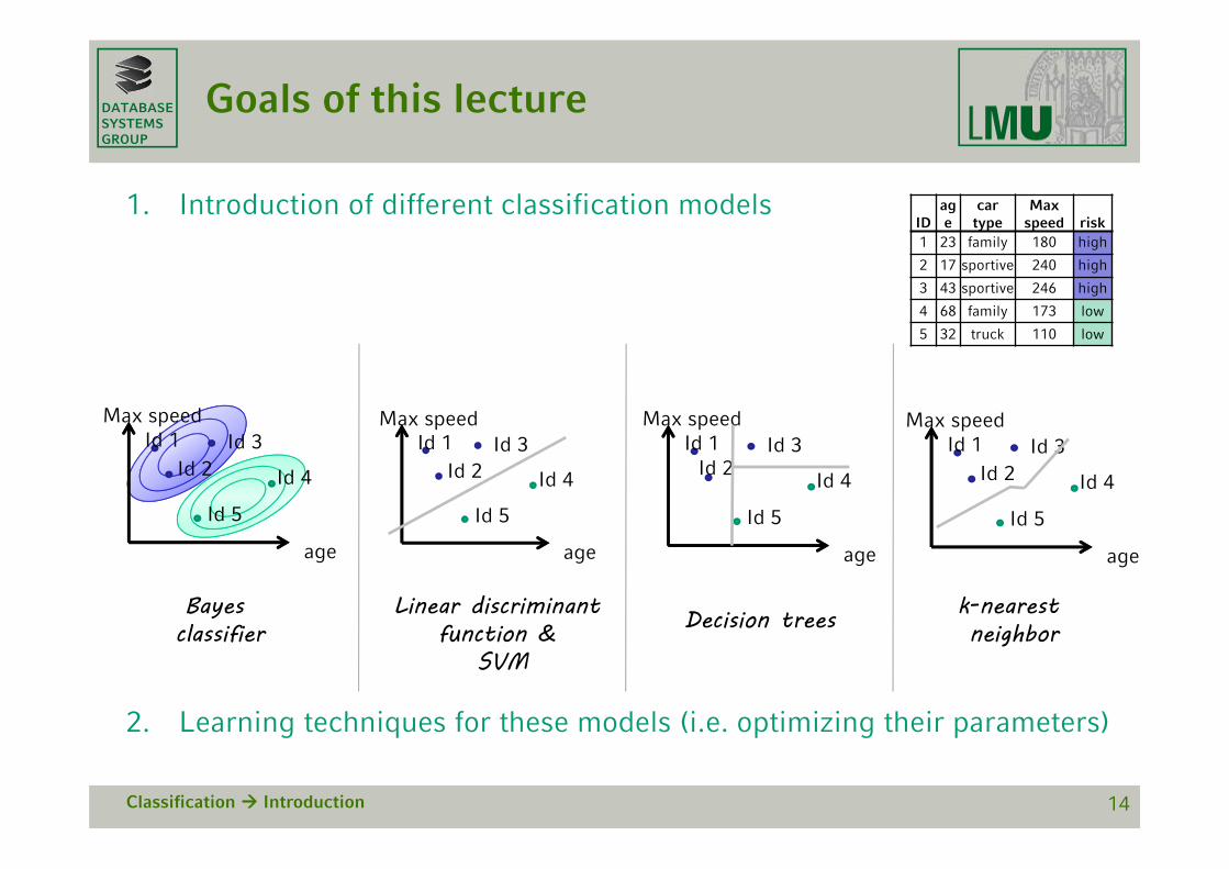
Goals of this lecture
1. Introduction of different classification models
2. Learning techniques for these models (i.e. optimizing their parameters)
Classification Introduction 14
IDage
car type
Max speed risk
1 23 family 180 high
2 17 sportive 240 high
3 43 sportive 246 high
4 68 family 173 low
5 32 truck 110 low
age
Max speedId 1
Id 2Id 3
Id 5
Id 4
age
Max speedId 1
Id 2Id 3
Id 5
Id 4
age
Max speedId 1
Id 2Id 3
Id 5
Id 4
Linear discriminant function &
SVM
Decision trees k-nearest neighbor
Bayes classifier
age
Max speedId 1
Id 2Id 3
Id 5
Id 4

DATABASESYSTEMSGROUP
Quality Measures for Classifiers
But before: How do we know that a classifier is “good”?
• Classification accuracy or classification error (complementary)
But also very important measures are:
• Compactness of the model– decision tree size; number of decision rules
• Interpretability of the model– Insights and understanding of the data provided by the model
• Efficiency– Time to generate the model (training time)
– Time to apply the model (prediction time)
• Scalability for large databases– Efficiency in disk-resident databases
• Robustness– Robust against noise or missing values
Classification Introduction 15

DATABASESYSTEMSGROUP
Evaluation of Classifiers – Notions
• Using training data to build a classifier and to estimate the model’s accuracy may result in misleading and overoptimistic estimates
WHY?
• We aim at a good accuracy for all objects from D, but the quality for
objects from D\O is unknown in general.
• The classifier K is optimized for O
• Applying K on objects from O will typically provide better results than
applying K to objects from D\O
• In other words: the results from the application of K to O is not a relaistic
view for the performance of applaying K to D
• This is called Overfitting
Classification Introduction 16
DATABASESYSTEMSGROUP
Evaluation of Classifiers – Notions
Solution:
• Train-and-Test: Decomposition of labeled data set into two partitions
– Training data is used to train the classifier• construction of the model by using information about the class labels
– Test data is used to evaluate the classifier• temporarily hide class labels, predict them as new and compare results
with original class labels
• Train-and-Test is not applicable if the set of objects for which the class label is known is very small
Classification Introduction 17

DATABASESYSTEMSGROUP
Evaluation of Classifiers –Cross Validation
• m-fold Cross Validation– Decompose data set evenly into m subsets of (nearly) equal size
– Iteratively use m – 1 partitions as training data and the remaining single partition as test data.
– Combine the m classification accuracy values to an overall classification accuracy, and combine the m generated models to an overall model for the data.
• Leave-one-out (aka “Jackknife”) is a special case of cross validation (m=n)– For each of the objects in the data set :
• Use set \ as training set
• Use the singleton set as test set
– Compute classification accuracy by dividing the number of correct predictions through the database size
– Particularly well applicable to nearest-neighbor classifiers
Classification Introduction 18

DATABASESYSTEMSGROUP
19
1 fold:1 a2 b
3 c
TestmengeKlassifikator
Trainingsmenge
Klassifikations-ergebnisse
1 a2 3 b c
Sei n = 3 : Menge aller Daten mit Klasseninformation die zu Verfügung stehen
2 fold:1 a3 c
2 b
TestmengeKlassifikator
Trainingsmenge
Klassifikations-ergebnisse
3 fold:2 b3 c
1 a
TestmengeKlassifikator
Trainingsmenge
Klassifikations-ergebnisse
Ablauf 3-fache Überkreuzvalidierung (3-fold Cross Validation)
gesamtesKlassifikations-
ergebnis
Example: Cross Validation
Knowledge Discovery in Databases I: Klassifikation

DATABASESYSTEMSGROUP
20
Evaluation of Classifiers –Cross Validation
Additional requirement: stratified folds• Proportionality of classes should be preserved
• Minimum requirement: each class should be present in O (i.e. in each fold)
• Better: class distributions in training and test set should represent the class distribution in D (or at least in O)
• Leaf-one-out is by designed NOT stratified
• Standard: 10-fold, stratified cross validation, repeated 10 times
Knowledge Discovery in Databases I: Klassifikation

DATABASESYSTEMSGROUP
21
Bewertung von Klassifikatoren
Alternative: Bootstrap
bilde Trainingsmenge durch Ziehen mit Zurücklegen.– jedes Sample hat die gleiche Größe wie die ursprüngliche
Trainingsmenge
– ein Sample enthält durchschnittlich 63% der Ausgangsbeispiele(einige mehrfach, etwa 37% gar nicht):
• ein einzelnes Beispiel in einem Datensatz mit n Beispielen hat bei jedem Ziehendie Chance 1/n gezogen zu werden, wird also mit Wahrscheinlichkeit 1-1/n nichtgezogen
• nach n-mal Ziehen ist ein bestimmtes Element mit Wahrscheinlichkeit
nicht gezogen worden
• für große n ist
– daher auch der Name “0.632 bootstrap” für diese Sampling-Methode
Achtung: Im Allgemeinen eher optimistische Fehlerschätzung
n
n
11
368.011 1
e
n
n
Knowledge Discovery in Databases I: Klassifikation
DATABASESYSTEMSGROUP
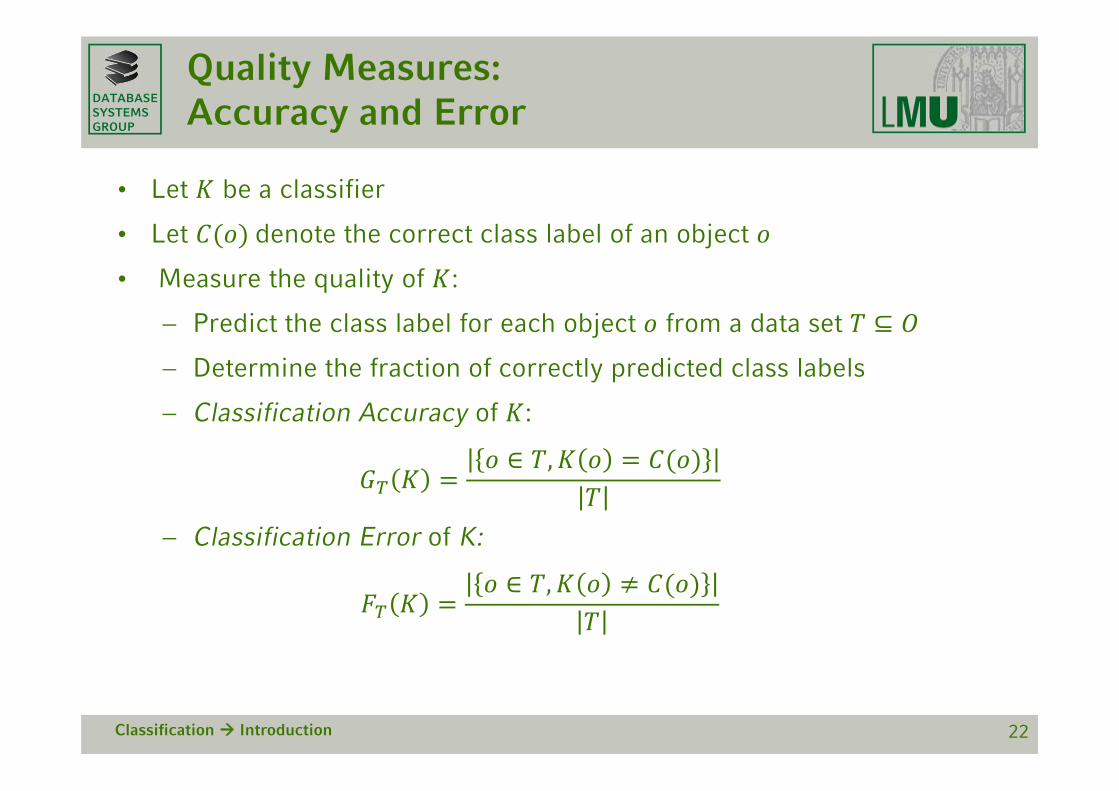
Quality Measures: Accuracy and Error
• Let be a classifier
• Let denote the correct class label of an object
• Measure the quality of :
Predict the class label for each object from a data set ⊆
Determine the fraction of correctly predicted class labels
Classification Accuracy of :
∈ ,
Classification Error of K:
∈ ,
Classification Introduction 22
DATABASESYSTEMSGROUP
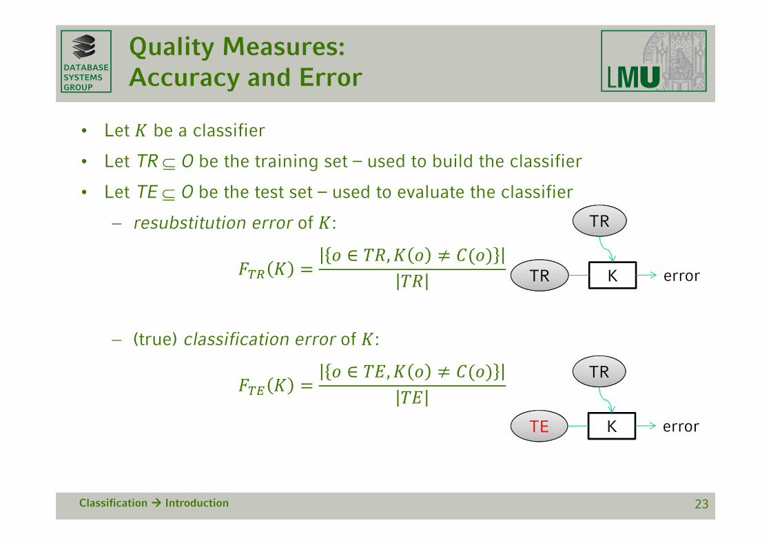
Quality Measures: Accuracy and Error
• Let be a classifier
• Let TR O be the training set – used to build the classifier
• Let TE O be the test set – used to evaluate the classifier
resubstitution error of :
∈ ,
(true) classification error of :
∈ ,
Classification Introduction 23
TR
TR K error
TR
TE K error

DATABASESYSTEMSGROUP
Quality Measures: Confusion Matrix
• Results on the test set: confusion matrix
• Based on the confusion matrix, we can compute several accuracymeasures, including:– Classification Accuracy, Classification Error
– Precision and Recall.
24
class1 class 2 class 3 class 4 other
class 1
class 2
class 3
class 4
other
35 1 1
0
3
1
3
31
1
1
50
10
1 9
1 4
1
1
5
2
210
15 13
classified as ...
corr
ect
clas
sla
bel.
..
correctly classifiedobjects
Knowledge Discovery in Databases I: Klassifikation

DATABASESYSTEMSGROUP
Quality Measures: Class of Interest
• Consider a classification problem with a so-called class of interest, i.e. where the main focus lies on classifying a particular class correctly.
• Example: A medical researcher wants to develop a test for early recognition of breast cancer– 1, 1 , where 1 corresponds to the women that have breast
cancer
– In this case, the ‘data-objects’ with 1 would be called positive objects or positive tuples while the others are called negative objects
• This leads to additional accuracy measures:
– recall (true positive rate):
– precision:
– specificity (true negative rate):
Classification Introduction 25
: positives: negatives: true positives: false positives

DATABASESYSTEMSGROUP
26
Quality Measures: Precision and Recall
|||)}()(|{|),(Precision
i
iTE K
oCoKKoiK
Knowledge Discovery in Databases I: Klassifikation
•Recall: fraction of test objects of class i, which have been identified correctly
• Let Ci= {o TE | C(o) = i}, then
•Precision: fraction of test objects assigned to class i, which have beenidentified correctly
•Let Ki= {o TE | K(o) = i}, then
|||)}()(|{|),(Recall
i
iTE C
oCoKCoiK
Ci
Ki
assigned class K(o)
corr
ect
clas
sC
(o) 1 2
12

DATABASESYSTEMSGROUP
Overfitting
• Characterization of overfitting:There are two classifiers K and K´ for which the following holds:– on the training set, K has a smaller error rate than K´
– on the overall test data set, K´ has a smaller error rate than K
• Example: Decision Tree
Classification Introduction 27
clas
sifi
cati
on a
ccur
acy
generalization classifier specialization
training data settest data set
“overfitting”
tree size

DATABASESYSTEMSGROUP
Overfitting (2)
• Overfitting– occurs when the classifier is too optimized to the (noisy) training data
Worst case: memorization (“Auswendiglernen”)
– As a result, the classifier yields worse results on the test data set
– Potential reasons• bad quality of training data (noise, missing values, wrong values)
• different statistical characteristics of training data and test data
• Overfitting avoidance– Removal of noisy and erroneous training data; in particular,
remove contradicting training data
– Choice of an appropriate size of the training set: not too small, not too large
– Choice of appropriate sample: sample should describe all aspects of the domain and not only parts of it
Classification Introduction 28

DATABASESYSTEMSGROUP
Underfitting
• Underfitting– Occurs when the classifiers model is too simple, e.g. trying to separate
classes linearly that can only be separated by a quadratic surface
– happens seldomly
• Trade-off – Usually one has to find a good balance between over- and underfitting
Classification Introduction 29
DATABASESYSTEMSGROUP
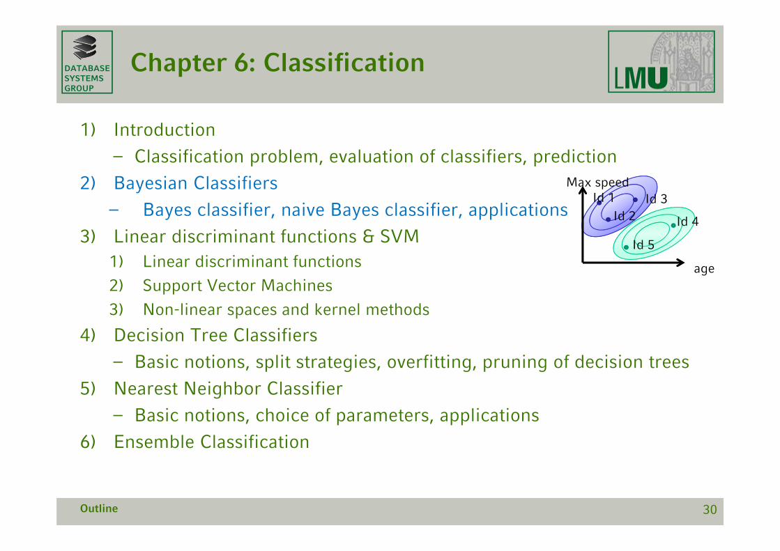
Chapter 6: Classification
1) Introduction
– Classification problem, evaluation of classifiers, prediction
2) Bayesian Classifiers
– Bayes classifier, naive Bayes classifier, applications
3) Linear discriminant functions & SVM1) Linear discriminant functions
2) Support Vector Machines
3) Non-linear spaces and kernel methods
4) Decision Tree Classifiers
– Basic notions, split strategies, overfitting, pruning of decision trees
5) Nearest Neighbor Classifier
– Basic notions, choice of parameters, applications
6) Ensemble Classification
Outline 30
age
Max speedId 1
Id 2Id 3
Id 5
Id 4

DATABASESYSTEMSGROUP
Bayes Classification
• Probability based classification– Based on likelihood of observed data, estimate explicit probabilities for
classes
– Classify objects depending on costs for possible decisions and the probabilities for the classes
• Incremental– Likelihood functions built up from classified data
– Each training example can incrementally increase/decrease the probability that a hypothesis (class) is correct
– Prior knowledge can be combined with observed data.
• Good classification results in many applications
Classification Bayesian Classifiers 31
DATABASESYSTEMSGROUP
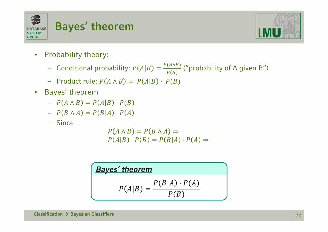
Bayes’ theorem
• Probability theory:
– Conditional probability: ∧
(“probability of A given B”)
– Product rule: ∧ ⋅ • Bayes’ theorem
– ∧ ⋅– ∧ ⋅– Since
∧ ∧ ⇒⋅ ⋅ ⇒
Classification Bayesian Classifiers 32
Bayes’ theorem
⋅
DATABASESYSTEMSGROUP
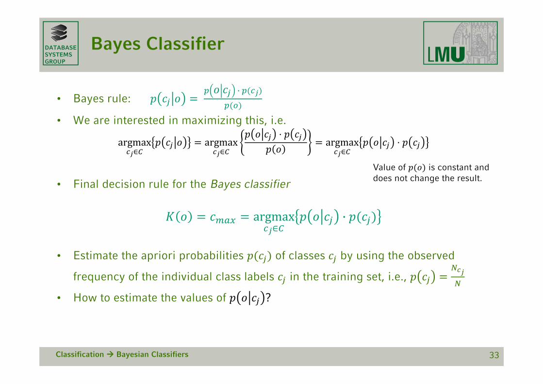
Bayes Classifier
• Bayes rule: ·
• We are interested in maximizing this, i.e.
argmax∈
argmax∈
⋅argmax
∈⋅
• Final decision rule for the Bayes classifier
argmax∈
·
• Estimate the apriori probabilities of classes by using the observed
frequency of the individual class labels in the training set, i.e.,
• How to estimate the values of ?
Classification Bayesian Classifiers 33
Value of is constant and does not change the result.

DATABASESYSTEMSGROUP
Density estimation techniques
• Given a database DB, how to estimate conditional probability ?– Parametric methods: e.g. single Gaussian distribution
• Compute by maximum likelihood estimators (MLE), etc.
– Non-parametric methods: Kernel methods• Parzen’s window, Gaussian kernels, etc.
– Mixture models: e.g. mixture of Gaussians (GMM = Gaussian Mixture Model)
• Compute by e.g. EM algorithm
• Curse of dimensionality often lead to problems in high dimensional data– Density functions become too uninformative
– Solution:• Dimensionality reduction
• Usage of statistical independence of single attributes (extreme case: naïve Bayes)
Classification Bayesian Classifiers 34
DATABASESYSTEMSGROUP
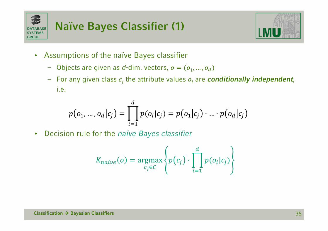
Naïve Bayes Classifier (1)
• Assumptions of the naïve Bayes classifier
– Objects are given as d-dim. vectors, 1, … ,
– For any given class the attribute values are conditionally independent, i.e.
, … , | ⋅ … ⋅
• Decision rule for the naïve Bayes classifier
argmax∈
⋅ |
Classification Bayesian Classifiers 35

DATABASESYSTEMSGROUP
Naïve Bayes Classifier (2)
• Independency assumption: , … , ∏ |
• If i-th attribute is categorical:| can be estimated as the relative frequency
of samples having value as -th attribute in class in the training set
• If i-th attribute is continuous:can, for example, be estimated through:
– Gaussian density function determined by , , ,
,e
,,
• Computationally easy in both cases
Classification Bayesian Classifiers 36
p(oi|c3)
xii,3
p(oi|c2)
xii,2
p(oi|c1)
xii,1
xi
p(oi|cj)
f(xi)
oi

DATABASESYSTEMSGROUP
Example: Naïve Bayes Classifier
• Model setup:– Age ~ , (normal distribution)
– Car type ~ relative frequencies
– Max speed ~ , (normal distribution)
Classification Bayesian Classifiers 37
ID age car type Max speed risk1 23 family 180 high2 17 sportive 240 high3 43 sportive 246 high4 68 family 173 low5 32 truck 110 low
Maxspeed:222, 36.49141.5, 44.54
Age:27.67, 13.6150, 25.45
Car type:
DATABASESYSTEMSGROUP
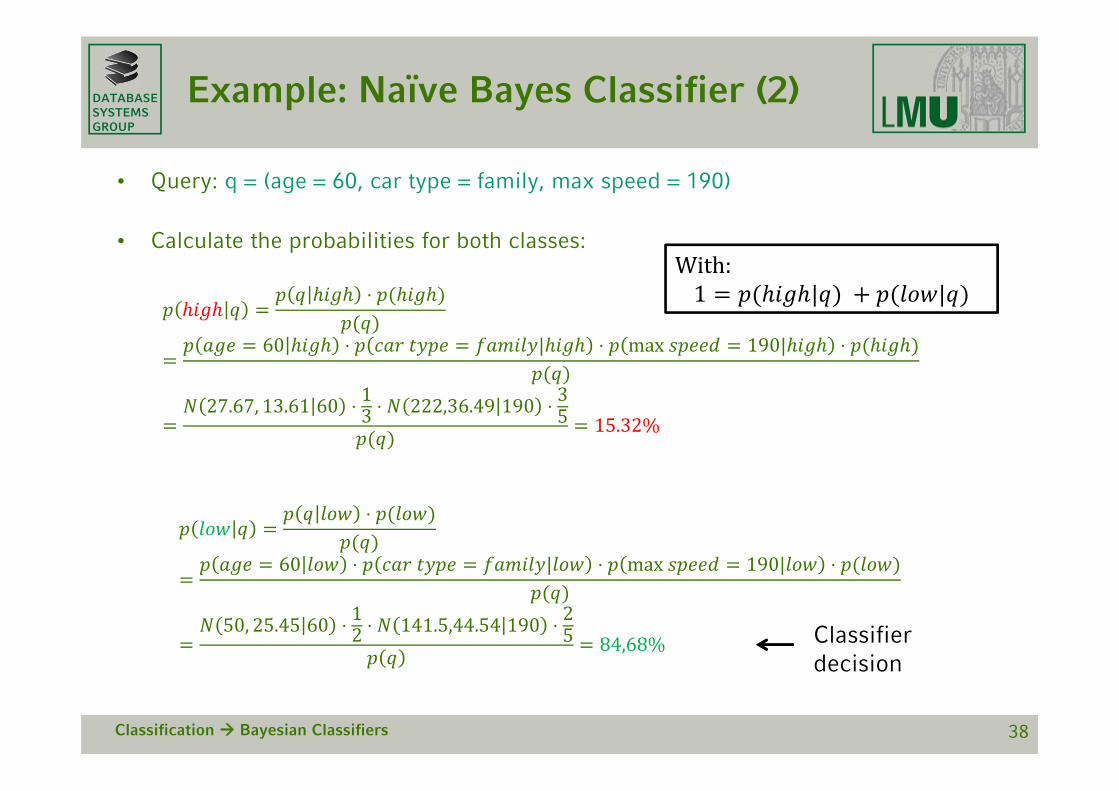
Example: Naïve Bayes Classifier (2)
• Query: q = (age = 60, car type = family, max speed = 190)
• Calculate the probabilities for both classes:
⋅
60 ⋅ | ⋅ max 190| ⋅
27.67, 13.61 60 ⋅ 13 ⋅ 222,36.49 190 ⋅ 35 15.32%
⋅
60 ⋅ | ⋅ max 190| ⋅
50, 25.45 60 ⋅ 12 ⋅ 141.5,44.54 190 ⋅ 25 84,68%
Classification Bayesian Classifiers 38
With:1 | |
Classifier decision
DATABASESYSTEMSGROUP
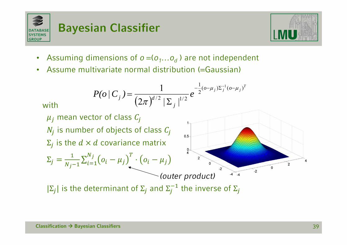
Bayesian Classifier
• Assuming dimensions of o =(o1…od ) are not independent
• Assume multivariate normal distribution (=Gaussian)
with
mean vector of class
is number of objects of class
Σ is the covariance matrix
Σ ∑ ⋅
|Σ | is the determinant of Σ and Σ the inverse of Σ
Classification Bayesian Classifiers 39
T
jjj oo
jdj e)CP(o
)()(21
2/12/
1
||21|
(outer product)
DATABASESYSTEMSGROUP
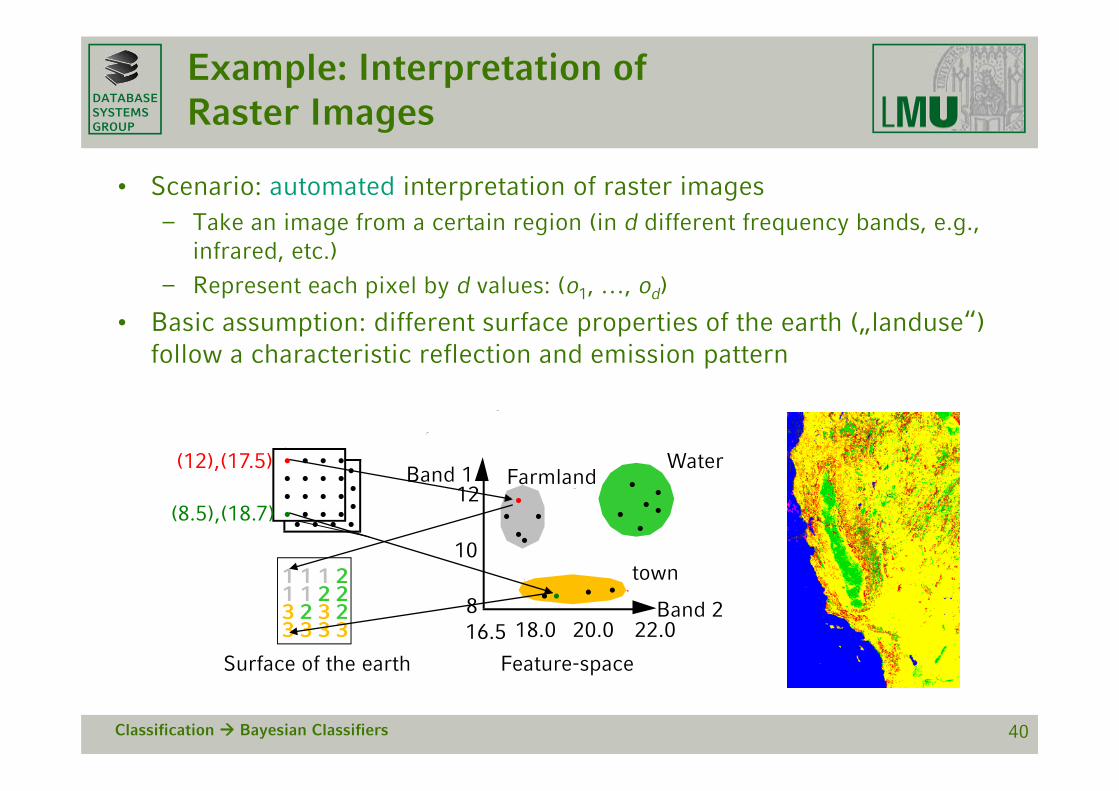
Example: Interpretation of Raster Images
• Scenario: automated interpretation of raster images– Take an image from a certain region (in d different frequency bands, e.g.,
infrared, etc.)
– Represent each pixel by d values: (o1, …, od)
• Basic assumption: different surface properties of the earth („landuse“) follow a characteristic reflection and emission pattern
Classification Bayesian Classifiers 40
• • • •• • • •• • • •• • • •
• • • •• • • •• • • •• • • •
Surface of the earth Feature-space
Band 1
Band 216.5 22.020.018.08
12
10
•
(12),(17.5)
••••
••• •
••
••••1 1 1 21 1 2 23 2 3 23 3 3 3
FarmlandWater
town
(8.5),(18.7)
DATABASESYSTEMSGROUP
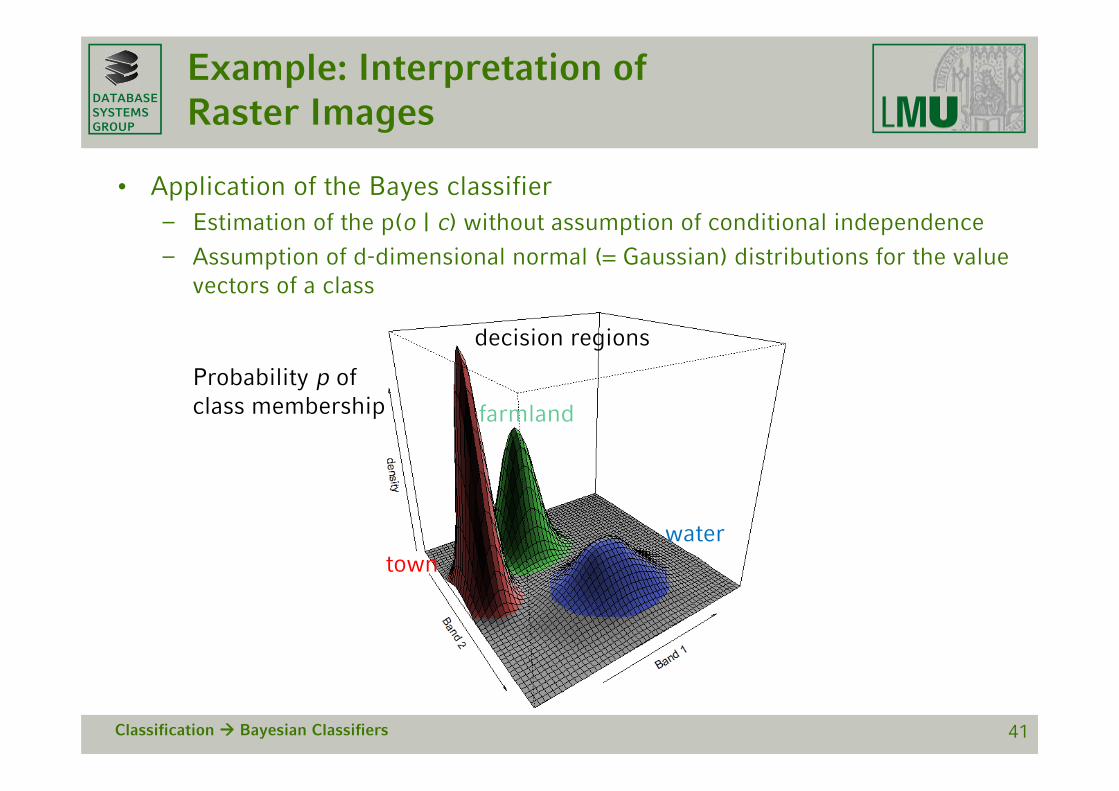
Example: Interpretation of Raster Images
• Application of the Bayes classifier– Estimation of the p(o | c) without assumption of conditional independence
– Assumption of d-dimensional normal (= Gaussian) distributions for the value vectors of a class
Classification Bayesian Classifiers 41
farmland
townwater
decision regions
Probability p ofclass membership

DATABASESYSTEMSGROUP
Example: Interpretation of Raster Images
• Method: Estimate the following measures from training data– : d-dimensional mean vector of all feature vectors of class
– Σ : covariance matrix of class
• Problems with the decision rule– if likelihood of respective class is very low
– if several classes share the same likelihood
Classification Bayesian Classifiers 42
unclassified regions
threshold
water
town
farmland
DATABASESYSTEMSGROUP
Bayesian Classifiers – Discussion
• Pro– High classification accuracy for many applications if density function
defined properly
– Incremental computation many models can be adopted to new training objects by updating densities
• For Gaussian: store count, sum, squared sum to derive mean, variance• For histogram: store count to derive relative frequencies
– Incorporation of expert knowledge about the application in the prior
• Contra– Limited applicability often, required conditional probabilities are not available
– Lack of efficient computation in case of a high number of attributes particularly for Bayesian belief networks
Classification Bayesian Classifiers 43
DATABASESYSTEMSGROUP
The independence hypothesis…
• … makes efficient computation possible
• … yields optimal classifiers when satisfied
• … but is seldom satisfied in practice, as attributes (variables) are often correlated.
• Attempts to overcome this limitation:– Bayesian networks, that combine Bayesian reasoning with causal
relationships between attributes
– Decision trees, that reason on one attribute at the time, considering most important attributes first
• Nevertheless, naïve Bayes is very often (surprisingly) good in practice
Classification Bayesian Classifiers 44