5

k-e Flow Modeling of Osmosis

• Cristiana Laranjeira • Luís Sanches-Fernandes • Amadeu Borges • • Nuno Cristelo* •

University of Trás-os-Montes e Alto Douro, PortugalCorresponding author

Abstract

Laranjeira, C., Sanches-Fernandes, L., Borges, A., & Cristelo, N. k-e Flow Modeling of Osmosis (September-October, 2015). Water Technology and Sciences (in Spanish), 6(5), 5-16.

Several measures have been taken to satisfy global water consumption needs. Desalination has been proven to be a viable solution and has therefore been increasingly used over the past two decades. This research is aimed at making a contribution through the use of numerical modeling to predict the behavior of laminar flow in desalination systems with an incompressible fluid (sea water). The study considered two scenarios— with and without a pressure-driven membrane, the latter enabling the study of the effects of gravity. The theoretical description of flow is based on mass, momentum and energy conservation equations. Computational fluid dynamics techniques were used to simulate flow according to different scenarios using ANSYS 12.1 software. The results show that the membrane significantly influences the flow process, with a significant impact in section x = 0.240 m when beginning to develop in the lower part of the cross-section.

Keywords: Desalination; Membrane; CFD modeling; ANSYS 12.1.

ISSN 0187-8336 • Tecnología y Ciencias del Agua, vol. VI, núm. 5, septiembre-octubre de 2015, pp. 5-16

Laranjeira, C., Sanches-Fernandes, L., Borges, A., & Cristelo, N. k-e flujo modelado de ósmosis (septiembre-octubre, 2015). Tecnología y Ciencias del Agua, 6(5), 5-16.

Con el fin de satisfacer las necesidades de agua de consumo a escala global se han tomado varias medidas. La desalinización ha demostrado ser una solución viable, y por lo tanto es una de las utilizadas cada vez más en las dos últimas décadas. Este trabajo de investigación pretende ser una contribución que emplea la modelización numérica para predecir el comportamiento de flujo laminar de un fluido incompresible (agua de mar) en los sistemas de desalinización. Dos escenarios diferentes se consideran: con y sin una membrana impulsada por presión. La última ha permitido estudiar los efectos de la gravedad. La descripción teórica del flujo se basa en las ecuaciones de conservación de masa, momento y energía. Se utilizaron técnicas de dinámica de fluidos computacional para simular el flujo en diferentes escenarios, utilizando el software ANSYS 12.1. Los resultados mostraron que la membrana tiene una influencia muy importante en el proceso de flujo, con un impacto importante de la sección x = 0.240 m, cuando se empieza a desarrollar hacia la zona inferior de la sección transversal.

Palabras clave: desalinización, membrana, modelado CFD, ANSYS 12.1.

Resumen

Received: 17/10/2011Accepted: 01/05/2015

Introduction

Desalination is a process used to remove salt and other minerals and/or chemicals from sea and brackish water, turning it into potable water ready for human consumption (Marcovecchio, Mussati, Aguirre, & Scena, 2005; Akgul, Çak-makci, Kayaalp, & Koyuncu, 2008; Charcosset, 2009; Ettouney & El-Dessouky, 2001; Greenlee, Lawler, Freeman, Marrot, & Moulin, 2009; Kha-

waji, Kutubkanah, & Wie, 2008). Karagiannis and Soldatos (2008) have classified desalination methods in two larger groups: thermic methods (phase-change processes) and membrane meth-ods (without phase-change). Fletcher and Wiley (2004) worked towards the development of a Computational Fluids Dynamic (CFD) model in order to accurately characterise the flow rate in the feed and permeable channels in membrane pressure-induced processes. The referred au-

6

Tecn

olog

ía y

Cie

ncia

s del

Agu

a, v

ol. V

I, nú

m. 5

, sep

tiem

bre-

octu

bre

de 2

015,

pp.

5-1

6Laranjeira et al . , k-e Flow Modeling of Osmosis

• ISSN 0187-8336

thors state that the flow rate in both channels is governed by the mass, momentum and mass of the solute fraction equations. These equations are presented in a cartesian coordinate system, considering that density, viscosity and diffuse-ness are a function of the solute fraction, and are similar to the ones used in previous work (Wiley & Fletcher, 2002, 2003; Alexiadis, Bao, Fletcher, Wiley, Clements, 2006), with the following modifications: to characterise the viscosity a set of related constants are included; gravitational forces are also included; mass is used instead of concentration, as in the formulation of the compressible flow, which guarantees mass con-servation of the solute. For the flow conditions considered, the density is only a function of the solute mass fraction, since the flow is regarded as isothermal and the dependency of the density pressure is extremely small, thus negligible. In this case, the density effects are included in every term of the equations of conservation, and thus the model is more general, ensuring strict mass conservation for all constitutive valid models (Fletcher & Wiley, 2004; Alexiadis et al., 2006; Wiley & Fletcher, 2002; Pa, Moham-madi, Hosseinalipour, & Allahdini, 2008). In this work, the filtration process was implemented by applying a pressure difference between the permeable and feed channels. The pressure dif-ference is used to determine the flow through the membrane, but the fact that the pressure is tens of bars higher in the feed channel has no effect on the hydrodynamics. Therefore, the reference pressure at the outlet of the two chan-nels is zero (p = 0) for computational purposes (only the pressure gradients are shown in the equations). This is a computational pattern to avoid loss of rounding error precision. Wardeh and Morvan (2008), using the same equations and channel geometry, made CFD simula-tions of flow and concentration polarisation in spacer-filled channels for water desalination. To model the selective transfer from the feeding to the permeable channel through the membrane surface they used finite element code ANSYS-CFX, and were able to show that a feed channel with spacer filaments reduces concentration

polarisation on the membrane surface and therefore fouling.

Mathematical model

Governing equations of fluid flow (mass, mo-mentum and energy equations) can be altered by factors like fluid condition (compressible or uncompressible), 2D or 3D flow, and others.

Flow equations

The following are the equations of continuity in two dimensions (1), momentum (2), and two dimensional, laminar and uncompressible flow on a regular cross-section channel with a membrane separating the feed and permeable channels (3). Equation (4) represents salt mass variation on flow. Note that the symbol glossary can be found at the end of the paper:

ux+

vy= 0 (1)

u2

x+

uvy

=px+ 2

xμux+xμ

uy+vx

23 x

μux+vy

gx (2)

uvx

+v2

y

=py+ 2

yμvy+yμ

uy+vx

23 y

μux+vy

gy (3)

umA

x+

vmA

y

=x

DABmA

x+y

DABmA

y (4)

7

Tecn

olog

ía y

Cie

ncia

s del

Agu

a, v

ol. V

I, nú

m. 5

, sep

tiem

bre-

octu

bre

de 2

015,

pp.

5-1

6

Laranjeira et al . , k-e Flow Modeling of Osmosis

ISSN 0187-8336 •

In equations (1), (2), (3) and (4) x and y are horizontal and vertical space coordinates, respectively; r is the density; m is the dynamic viscosity; g is the gravitational acceleration; D is the diffuseness, and mA the salt mass percentage.

Boundary conditions

Boundary conditions are applied to the walls, membrane, and initial and final cross-section of the channels. Velocity through the membrane is defined using continuity equation (5):

Qw =Qp

Aw uw = Ap up (5)

The flow rate in the system is divided in the flow that remains in the feed channel (Qw) and the flow that reaches the permeable channel through the membrane (Qp). Therefore, the infil-tration velocity through the membrane (vw) was obtained considering that the permeable flow equals the flow that goes through the membrane area (Awm) (6):

vw =Ap upAwm

(6)

Exiting pressure on the feed channel is defined as being the same as in the case of non-existence of the membrane (7):

p = 0 (7)

Hence, the exiting pressure on the perme-able channel, when considering the existence of the membrane, equals the difference between the feed and permeable channels’ pressure, obtained using Bernoulli’s equation (8), which relates pressure with velocity u and head H at any point on the flow line considered:

H =p+u2

2g+ z (8)

The boundary condition at the start of the channel completely defines the velocity profile and the salt mass percentage in the water (9):

u = 6u yh1 yh

v = 0

mA =mA0 (9)

For the walls the flow conditions apply (10):

u = 0

v = 0

mA

y= 0 (10)

At the membrane, on the feed channel side, tangent velocity is defined as zero (no flow is considered) and the infiltration velocity is speci-fied (11):

u = 0

v = vw (11)

On the permeable channel, the infiltration velocity at the membrane is corrected to account for the change in density, therefore keeping the flow rate through the membrane constant (12):

u = 0

v = vp = vw w

p

(12)

Experimental

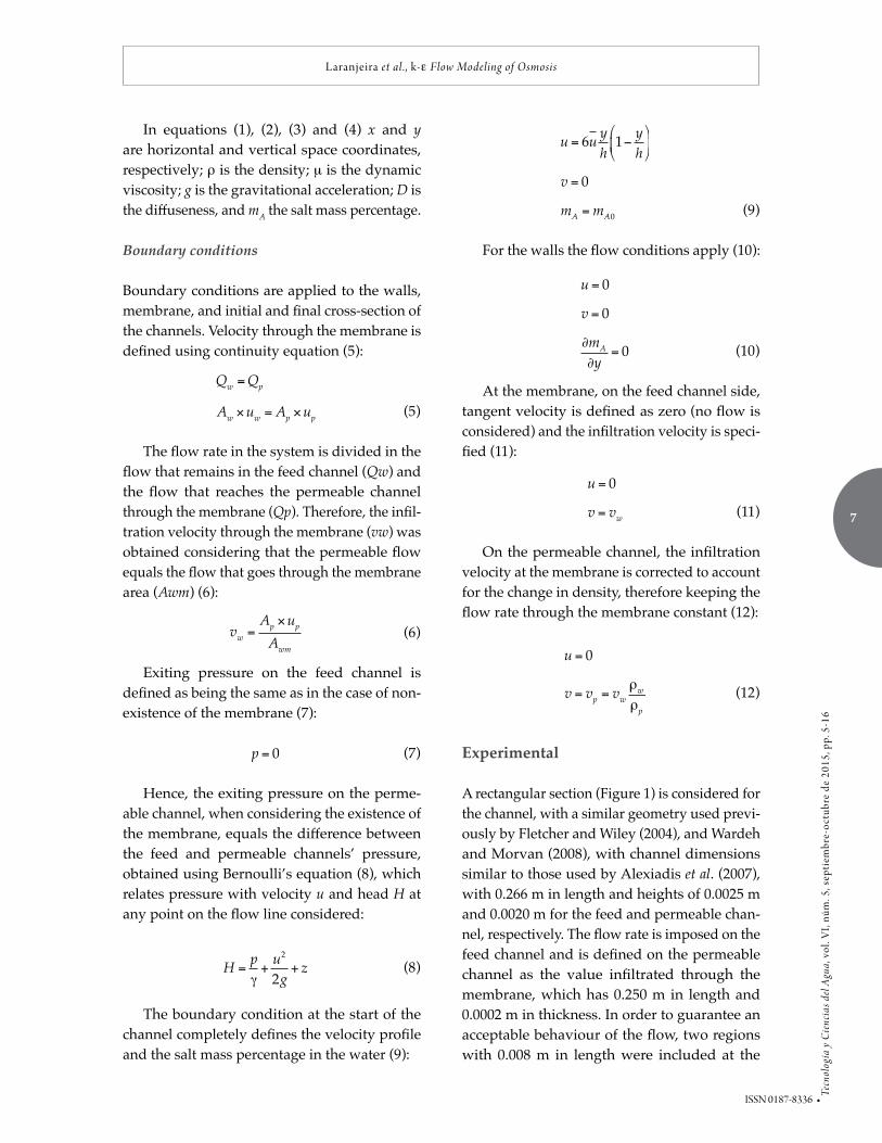
A rectangular section (Figure 1) is considered for the channel, with a similar geometry used previ-ously by Fletcher and Wiley (2004), and Wardeh and Morvan (2008), with channel dimensions similar to those used by Alexiadis et al. (2007), with 0.266 m in length and heights of 0.0025 m and 0.0020 m for the feed and permeable chan-nel, respectively. The flow rate is imposed on the feed channel and is defined on the permeable channel as the value infiltrated through the membrane, which has 0.250 m in length and 0.0002 m in thickness. In order to guarantee an acceptable behaviour of the flow, two regions with 0.008 m in length were included at the

8

Tecn

olog

ía y

Cie

ncia

s del

Agu

a, v

ol. V

I, nú

m. 5

, sep

tiem

bre-

octu

bre

de 2

015,

pp.

5-1

6Laranjeira et al . , k-e Flow Modeling of Osmosis

• ISSN 0187-8336

entering and exiting, for which previously de-scribed boundary conditions for entering and exiting sections were applied.

The solution considered in the simulations was composed of water with a salt mass of 0.002 kg/kg. The physical properties of the fluid vary with salt mass percentage and were defined by equations (13) and (14):

μ = 0.89 10 3 1.0+1.63mA( ) (13)

= 997.1 1.0+0.696mA( ) (14)

In which mA is the salt mass percentage (kg per solution kg); m is the dynamic viscosity (N/m2s), and r is the density (kg/m3).

Considering the mentioned channel, four simulations were executed with the conditions described in Table 1.

ANSYS CFD 12.1 (2010) software was used to perform fluid flow simulations during this research work. It is a Computational Fluid Dynamics software that combines pre- and post-processing with a powerful solving capacity.

Results and Discussion

Simulation without Membrane

Longitudinal Velocity Profile

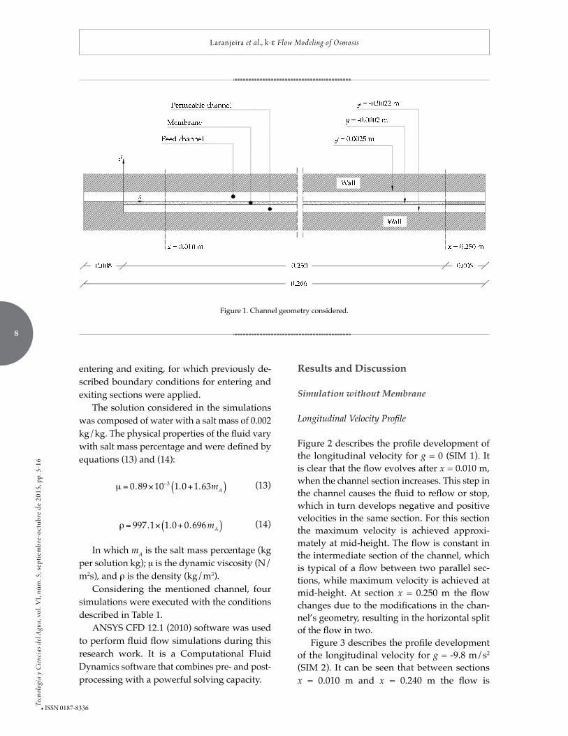
Figure 2 describes the profile development of the longitudinal velocity for g = 0 (SIM 1). It is clear that the flow evolves after x = 0.010 m, when the channel section increases. This step in the channel causes the fluid to reflow or stop, which in turn develops negative and positive velocities in the same section. For this section the maximum velocity is achieved approxi-mately at mid-height. The flow is constant in the intermediate section of the channel, which is typical of a flow between two parallel sec-tions, while maximum velocity is achieved at mid-height. At section x = 0.250 m the flow changes due to the modifications in the chan-nel’s geometry, resulting in the horizontal split of the flow in two.

Figure 3 describes the profile development of the longitudinal velocity for g = -9.8 m/s2 (SIM 2). It can be seen that between sections x = 0.010 m and x = 0.240 m the flow is

Figure 1. Channel geometry considered.

9

Tecn

olog

ía y

Cie

ncia

s del

Agu

a, v

ol. V

I, nú

m. 5

, sep

tiem

bre-

octu

bre

de 2

015,

pp.

5-1

6

Laranjeira et al . , k-e Flow Modeling of Osmosis

ISSN 0187-8336 •

Figure 2. Longitudinal velocity profile for g = 0.

Table 1. Conditions of the performed simulations.

SimulationsConditions

u(m/s) v(m/s) p(N/m2) g(m/s2) Membrane

SIM 1 0.1 0 0 0 No

SIM 2 0.1 0 0 -9.8 No

SIM 3 0.1 0 0 +9.8 No

SIM 4 0.1 0 0 -9.8 Yes

SIM 1, 2 and 3 were included with the objective of studying the influence of gravitational acceleration on fluid flow and, as such, no membrane was considered. SIM 4 included the membrane and therefore only the more realistic case of g = - 9.8 m/s2 was considered.

constant, typical of a laminar flow, without any significant changes in velocity. Maximum velocity is registered for almost the entire cross-section, diminishing only near the top and bottom. For this simulation, as in the case of the remaining simulations, the presence of the horizontal wall at section x = 0.250 m divides the flow in two. There is a slight increase in velocity at this section and at section x = 0.254 m (6.5 and 14.0%, respectively), regarding the

velocity at intermediate sections. At section x = 0.254 m, and contrary to what happens at section x = 0.250 m (although the difference is not significant), flow is more intense by the inferior solid wall of the channel.

The profile development of the longitu-dinal velocity for g = +9.8 m/s2 (SIM 3) was very similar to SIM 1 and therefore Figure 2 is used to analyse SIM3. Maximum velocity and reflow/stopping of the fluid occurred at section

10

Tecn

olog

ía y

Cie

ncia

s del

Agu

a, v

ol. V

I, nú

m. 5

, sep

tiem

bre-

octu

bre

de 2

015,

pp.

5-1

6Laranjeira et al . , k-e Flow Modeling of Osmosis

• ISSN 0187-8336

x = 0.010 m, typical laminar flow at the inter-mediate sections of the channel and split in two flows at section x = 0.250 m due to the horizontal wall.

In short, for SIM 1 and SIM 3 velocity is maximum at section x = 0.010 m, while for SIM 2 the highest velocity is achieved at the last sec-tion analysed (x = 0.254 m).

Normal Velocity Profile

Figure 4 describes the profile development of the velocity normal to the channel wall for g = 0 (SIM 1). As can be seen, at section x = 0.010 m the flow shows simultaneously positive and negative normal velocity, consequence of the reflow / stopping shown in Figure 2.

Intermediate sections’ results are not presented since they are approximately zero, with only a small flow development at section x = 0.060 m. However, at section x = 0.250 m, where the channel splits, there is a significant

flow development resulting in maximum veloc-ity values (both positive and negative) near the separation walls of the channel. The following section shows a less developed flow, with reduc-tions in the maximum velocities, regarding the previous section, of 93 and 60% for positive and negative values, respectively.

SIM 2 revealed a practically horizontal flow along the entire length of the channel, with the exception at section x = 0.250 m. This is due to the fact that the normal component of the velocity, right at the first section (x = 0.010 m) and beyond, is practically zero. For this reason the results for these sections are not presented. The exception is section x = 0.250 m, where the channel splits and the flow shows a very intense development, with equal positive and negative velocity values.

SIM 3 showed the highest influence on nor-mal velocity. At section x = 0.010 m of the flow development (Figure 4) normal velocity has positive and negative values, consequence of

Figure 3. Longitudinal velocity profile for g = -9.8 m/s2.

11

Tecn

olog

ía y

Cie

ncia

s del

Agu

a, v

ol. V

I, nú

m. 5

, sep

tiem

bre-

octu

bre

de 2

015,

pp.

5-1

6

Laranjeira et al . , k-e Flow Modeling of Osmosis

ISSN 0187-8336 •

the reflow / stopping of the fluid. Once again, at section x = 0.250 m, two different flows are cre-ated, with positive normal velocity near the top side of the horizontal separation wall and nega-tive normal velocity near the bottom side of the separation wall. Maximum positive and nega-tive velocities are achieved at this same section. It is possible to conclude that the flow develops nearer the top wall of the channel, possibly due to the fact that g has upwards orientation. The immediate section shows a less developed flow, with positive and negative velocities 77 and 82% lower, relatively to the previous section.

As can be seen from SIM 1, 2 and 3 the nor-mal velocity profiles only show variations at the extreme sections, being approximately constant for the remaining of the channel, indicating an almost horizontal flow surface. At section x = 0.254 m, where normal velocity peaks for

positive and negative values, the flow shows a similar configuration in all three simulations. However, for SIM 1 flow development is more pronounced near the bottom side of the separa-tion wall, for SIM 2 no difference in flow was detected between top and bottom sides and for SIM 3 the flow development is more pro-nounced near the top side.

Pressure Profile along the Channel

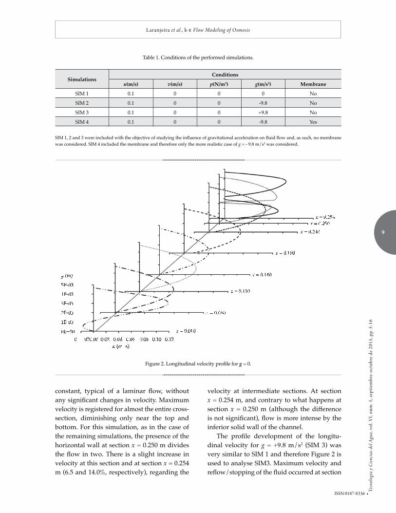
Figure 5 shows a comparative profile of the pressure along the channel for the three simu-lations without membrane: g = 0, g = -g and g = +g. Flow is laminar and therefore has a low Reynolds number, leading to an approximately zero difference in pressure (Dp ≈ 0). Therefore, only the sections where the pressure variations were more significant were analysed. The first

Figure 4. Normal velocity profile for g = 0.

12

Tecn

olog

ía y

Cie

ncia

s del

Agu

a, v

ol. V

I, nú

m. 5

, sep

tiem

bre-

octu

bre

de 2

015,

pp.

5-1

6Laranjeira et al . , k-e Flow Modeling of Osmosis

• ISSN 0187-8336

of these sections (x = 0.010 m) shows a similar pressure profile for SIM 1 and 3, with practically the same values. Pressure in these simulations is 73% less than in SIM 2. At section x = 0.250 m, where the maximum pressure point occurs at mid-height (the mid-height fluid’s longitudinal velocity was stopped by the horizontal wall starting at section x = 0.250 m), the variation in pressure is very significant. The pressure value at this point is 7% higher in SIM 2 than in SIM 3.

Simulation with Membrane

Longitudinal Velocity Profile

Figure 6 shows the development of the lon-gitudinal velocity profile in the channel with membrane (SIM 4). This development is par-ticularly noticeable at section x = 0.010 m, in a similar situation occurred with simulations 1 and 3 without membrane. Again, at this section

the fluid reflows or stops, increasing positive and negative velocities at the same time. The velocities also show very similar values to those obtained from SIM 1 and 3, reaching maximum value at mid-section.

At section x = 0.240 m flow starts to adopt a different behaviour, and at section x = 0.250 m, where the channel splits horizontally and two new flows are formed, the longitudinal velocity takes positive values near the bottom side of the separation wall and negative values near the top side. At this point the flow occurs preferably near the bottom of the channel, reaching its maximum value at the last section. In SIM 4 it is clear the flow development at section x = 0.010, immediately after the increase in the channel’s cross section, which is contrary to what was found during SIM 2, in which the flow is constant and the velocity is maximum at almost the entire height of the channel.

Figure 5. Pressure profile for g = 0, g = -9.8 m/s2 and g = +9.8 m/s2.

13

Tecn

olog

ía y

Cie

ncia

s del

Agu

a, v

ol. V

I, nú

m. 5

, sep

tiem

bre-

octu

bre

de 2

015,

pp.

5-1

6

Laranjeira et al . , k-e Flow Modeling of Osmosis

ISSN 0187-8336 •

Figure 6. Longitudinal velocity profile considering the membrane.

Normal Velocity Profile

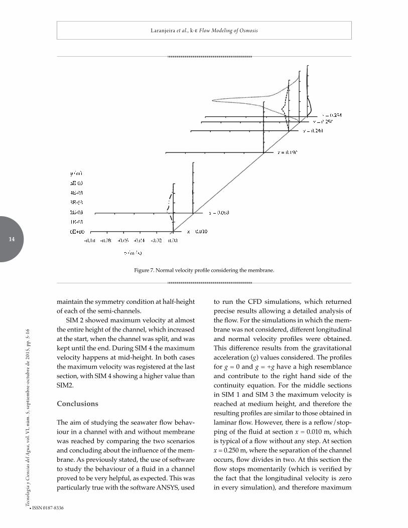
Figure 7 describes the profile development of the velocity normal to the channel wall consid-ering the membrane (SIM 4). As can be seen, at section x = 0.010 m the flow development presents only negative normal velocity, with a small percentage of the cross-section of the channel showing zero velocity, consequence of the reflow/stopping of the fluid observed in Figure 6. Middle sections of the channel are not presented since velocity values are approxi-mately zero, showing only a small flow devel-opment at sections x = 0.060 m and x = 0.190 m. At section x = 0.240 m and beyond it is clear that the existence of the membrane completely changed flow behaviour. In the case of SIM 1, 2 and 3 (Figure 4), the flow reaches maximum positive and negative velocities at section x = 0.250 m, in the proximity of the top and bottom sides of the horizontal separation wall

of the channel, respectively. In this case (SIM 4) there is no positive/negative velocity symmetry; there is instead a maximum positive velocity at the height of the separation wall. The immediate following section shows a less developed flow, only visible near the bottom of the channel, with a positive normal velocity.

In general, the profiles show negative values. However, there is an unusually high value at x = 0.250 m, which can only be explained by the near presence of the end of the membrane, where the wall is no longer permeable and, and as consequence, two separate flows start to develop, as illustrated in Figure 1. It should also be taken into account the near symmetry of the profile around the point of separation of the two flows. After this point, the upper flow has almost zero vertical speed, keeping the negative feature, but the lower flow behaviour is now positive, due to the lower flow rate. Note that both flows, after the end of the membrane,

14

Tecn

olog

ía y

Cie

ncia

s del

Agu

a, v

ol. V

I, nú

m. 5

, sep

tiem

bre-

octu

bre

de 2

015,

pp.

5-1

6Laranjeira et al . , k-e Flow Modeling of Osmosis

• ISSN 0187-8336

maintain the symmetry condition at half-height of each of the semi-channels.

SIM 2 showed maximum velocity at almost the entire height of the channel, which increased at the start, when the channel was split, and was kept until the end. During SIM 4 the maximum velocity happens at mid-height. In both cases the maximum velocity was registered at the last section, with SIM 4 showing a higher value than SIM2.

Conclusions

The aim of studying the seawater flow behav-iour in a channel with and without membrane was reached by comparing the two scenarios and concluding about the influence of the mem-brane. As previously stated, the use of software to study the behaviour of a fluid in a channel proved to be very helpful, as expected. This was particularly true with the software ANSYS, used

to run the CFD simulations, which returned precise results allowing a detailed analysis of the flow. For the simulations in which the mem-brane was not considered, different longitudinal and normal velocity profiles were obtained. This difference results from the gravitational acceleration (g) values considered. The profiles for g = 0 and g = +g have a high resemblance and contribute to the right hand side of the continuity equation. For the middle sections in SIM 1 and SIM 3 the maximum velocity is reached at medium height, and therefore the resulting profiles are similar to those obtained in laminar flow. However, there is a reflow/stop-ping of the fluid at section x = 0.010 m, which is typical of a flow without any step. At section x = 0.250 m, where the separation of the channel occurs, flow divides in two. At this section the flow stops momentarily (which is verified by the fact that the longitudinal velocity is zero in every simulation), and therefore maximum

Figure 7. Normal velocity profile considering the membrane.

15

Tecn

olog

ía y

Cie

ncia

s del

Agu

a, v

ol. V

I, nú

m. 5

, sep

tiem

bre-

octu

bre

de 2

015,

pp.

5-1

6

Laranjeira et al . , k-e Flow Modeling of Osmosis

ISSN 0187-8336 •

pressure is reached. Regarding the simulations without membrane, SIM 2 (g = -g) is the closest to reality since gravitational force is considered downwards. The flow is laminar and therefore shows a low Reynolds number, which results in an approximately zero difference in pressure (Dp ≈ 0). Overall, it can be concluded that the membrane has a significant influence on flow development. This influence is especially notori-ous at section x = 0.240 m and beyond, where flow starts to develop more towards the bottom area of the cross-section. At section x = 0.250 m, and according with the longitudinal velocity values, the flow runs almost entirely near the bottom of the channel. Also, based on normal velocity, flow develops in a symmetrical pat-tern, with maximum velocity at the horizontal separation wall of the channel.

Symbols

Aw – Area of the feed channel (m2/m). Ap – Area of the permeable channel (m2/m). u – Average initial velocity on the feed chan-

nel (m/s).V – Average velocity along the channel

(m/s).D – Difusity (m2/s).m – Dynamic viscosity (N/m2 s). h – Feed channel height (m). vw – Filtration velocity (m/s). Qw – Flow rate on the feed channel (m3/s). Qp – Flow rate on the permeable channel

(m3/s). g – Gravitational acceleration (m/s). x – Longitudinal direction.u – Longitudinal velocity (along the channel)

(m/s). Awm – Membrane area (m2/m). y – Normal direction.v – Normal velocity (normal to the mem-

brane) (m/s). p – Pressure (N/m2). DP – Pressure difference through the mem-

brane.mA – Salt mass percentage (kg/kg). r – Sea water density (kg/m3).

rw – Sea water density on the feed channel (kg/m3).

rp – Sea water density on the permeable channel (kg/m3).

uw – Velocity on the feed channel (m/s). up – Velocity on the permeable channel (m/s). g – Water density (kg/m3).

Acknowledgements

This work is supported by national funds by FCT-Portugue-

se Foundation for Science and Technology, under the project

UID/AGR/04033/2013.

References

Akgul, D., Çakmakci, M., Kayaalp, N., & Koyuncu, I. (2008). Cost Analysis of Seawater Desalination with Reverse Osmosis in Turkey. Desalination, 220, 123-131.

Alexiadis, A., Bao, J., Fletcher, D. F., Wiley, D. E., & Clements, D.J. (2006). Dynamic Response of a High-Pressure Reverse Osmosis Membrane Simulation of Time Dependent Disturbances. Desalination, 191, 397-403.

Alexiadis, A., Wiley, D. E., Vishnoi, A., Lee, R. H. K., Fletcher, D. F., & Bao, J. (2007). CFD Modeling of Reverse Osmosis Membrane Flow and Validation with Experimental Results. Desalination, 217, 242-250.

ANSYS 12.1, ANSYS Tutorials, 2010. Charcosset, C. (2009). A Review of Membrane Processes and

Renewable Energies for Desalination. Desalination, 245, 214-231.

Ettouney, H., & El-Dessouky, H. (2001). Teaching Desalination. Desalination, 141, 109-127.

Fletcher, D. F., & Wiley, D.E. (2004). A Computational Fluids Dynamics Study of Buoyancy Effects in Reverse Osmosis. Journal of Membrane Science, 245, 175-181.

Greenlee, L. F, Lawler, D. F., Freeman, B. D., Marrot, B., & Moulin, P. (2009). Reverse Osmosis Desalination: Water Sources, Technology, and Today’s Challenges. Water Research, 43, 2317-2348.

Karagiannis, I. C., & Soldatos, P. G. (2008). Water Desalination Cost Literature: Review and Assessment. Desalination, 223, 448-456.

Khawaji, A. D., Kutubkanah, I. K., & Wie, J. M. (2008). Advances in Seawater Desalination Technologies. Desalination, 221, 47-69.

Marcovecchio, M. G., Mussati, S. F., Aguirre, P. A., & Scena, N. J. (2005). Optimization of Hybrid Desalination Processes Including Multi Stage Flash and Reverse Osmosis Systems. Desalination, 182, 111-122.

16

Tecn

olog

ía y

Cie

ncia

s del

Agu

a, v

ol. V

I, nú

m. 5

, sep

tiem

bre-

octu

bre

de 2

015,

pp.

5-1

6Laranjeira et al . , k-e Flow Modeling of Osmosis

• ISSN 0187-8336

Pak, A., Mohammadi, T., Hosseinalipour, S. M., & Allahdini, V. (2008). CFD Modeling of Porous Membranes. Desalination, 222, 482-488.

Wardeh, S., & Morvan, H.P. (2008). CFD Simulations of Flow and Concentration Polarization in Spacer-Filled Channels for Application to Water Desalination. Chemical Engineering Research and Design, 86, 1107-1116.

Wiley, D. E., & Fletcher, D.F. (2003). Techniques for Computational Fluid Dynamics Modeling of Flow in Membrane Channels. Journal of Membrane Science, 211, 127-137.

Wiley, D. E., & Fletcher, D.F. (2002). Computational Fluid Dynamics Modeling of Flow and Permeation of Pressure-Driven Membrane Processes. Desalination, 145, 183-186.

Author’s institutional address

MSc. Cristiana LaranjeiraPhD. Luís FernandesPhD. Amadeu BorgesPhD. Nuno Cristelo

University of Trás-os-Montes e Alto Douro (UTAD)Quinta de Prados, Engenharias I, 5000-801 Vila Real, Portugal

Phone: +35 (125) 9350 356Fax: +35 (125) 9350 356cris.pfl@gmail. com lfilipe@utad.ptamadeub@utad.pt ncristel@utad.pt