June, 1995

PANEL COINTEGRATION;

ASYMPTOTIC AND FINITE SAMPLE PROPERTIES OF POOLED TIME SERIES TESTS WITH AN APPLICATION TO THE PPP HYPOTHESIS

Peter Pedroni

Indiana University

mailing address: Economics, Indiana University Bloomington, IN 47405

(812) 855-7925

email: PPEDRONI@INDIANA.EDU

*This is a substantially revised version of the draft that was presented at the North American and EuropeanEconometric Society Meetings in Quebec and Maastricht respectively during the summer of 1994, whose participants Ithank for their many helpful comments. I also thank especially Richard Clarida, Heejoon Kang, Andrew Levin, MasaoOgaki, David Papell and Pierre Perron for helpful suggestions, and Rasmus Ruffer and Younghan Kim for valuableresearch assistance.

Abstract

This paper studies asymptotic and finite sample properties of statistics devised to test for the null of no

cointegration in nonstationary pooled time series panels as both the cross section and time series dimensions

grow large. The paper finds that for panels with homogenous long run parameters, the spurious regression

coefficient estimates become consistent even under the null of no cointegration, and this generates a

superconsistency result for panels whereby it becomes irrelevant for the asymptotic distributions whether the

residuals are known or are estimated. For heterogenous panels, on the other hand, this asymptotic

equivalency does not hold, and the use of stationarity tests that are convergent for raw data can even become

divergent when applied to estimated residuals. Furthermore, the direct use of unit root tests for estimated

residuals can generate data dependencies that are not present in unit root statistics that are applied to raw

panel data. The paper therefore derives asymptotic distributions for panel cointegration statistics that

circumvent these problems, and also reports on finite sample properties of these statistics based on Monte

Carlo simulations for a varying number of time periods and cross sections. These statistics allow for

complete heterogeneity of the dynamics and potential cointegrating relationships across members of the

panel. Finally, an empirical application of these panel cointegration statistics is demonstrated for the

purchasing power parity hypothesis, which has been difficult to evidence on the basis of conventional single

series cointegration tests.

1

PANEL COINTEGRATION;ASYMPTOTIC AND FINITE SAMPLE PROPERTIES OF POOLED

TIME SERIES TESTS WITH AN APPLICATION TO THE PPP HYPOTHESIS

I. Introduction

The use of cointegration techniques to test for the presence of long run relationships among

integrated variables have enjoyed growing popularity in the empirical literature. Unfortunately, a

common dilemma for practitioners has been the inherently low power of many of these tests when

applied to time series available for the length of the post war period. Research by Shiller and

Perron (1985), Perron (1989,1991) and recently Pierse and Snell (1995) have generally confirmed

that it is the span of the data, rather than frequency that matters for the power of these tests. On

the other hand, expanding the time horizon to include pre-war data can risk introducing unwanted

changes in regime for the data relationships. In light of these data limitations, it is natural to

question whether a practical alternative might not be to bring additional data to bear upon a

particular cointegration hypothesis by drawing upon data from among similar cross sectional data

in lieu of additional time periods.

For many important hypotheses to which cointegration methods have been applied, data is

in fact commonly available on a time series basis for multiple countries, for example, and

practitioners could stand to benefit significantly if there existed a straightforward manner in which

to perform cointegration tests for pooled time series panels. Many areas of research come to

mind, such as the growth and convergence literature, or the purchasing power parity literature, for

which it is natural to think about long run time series properties of data that are expected to hold

for groups of countries. Alternatively, examples are also readily available for issues that involve

time series panels for yields across asset term structures or price movements across industries, to

name only a few. For applications where the cross sectional dimension grows reasonably large,

existing systems methods such as the Johansen (1989, 1991) procedure are likely to become

infeasible, and panel methods may be more appropriate.

On the other hand, pooling time series has traditionally involved a substantial degree of

2

See for example Holz-Eakon, Newey and Rosen (1988) on the dynamic homogeneity1

restrictions required typically for the implementation of panel VAR techniques.

For example, Levin and Lin show by Monte Carlo simulation that at a nominal size of2

10%, with 100 time periods the power of pooled unit root tests jump to nearly 100% for 25 crosssections against stationarity alternates with heterogenous means and heterogenous means andtrends as compared to 31% and 37% respectively for the conventional single series tests.

sacrifice in terms of the permissible heterogeneity of the individual time series. In order to ensure1

broad applicability of any panel cointegration test, it will be important to allow for as much

heterogeneity as possible among the individual members of the panel. Therefore, one objective of

this paper will be to construct panel cointegration test statistics that allow one to vary the degree

of permissible heterogeneity among the members of the panel, and in the extreme case pool only

the multivariate unit root information, leaving the form of the time series dynamics and the

potential cointegrating vectors entirely heterogeneous across individual members.

Unfortunately, very little is known about the properties of cointegration tests for these

types of applications in which both the time series and cross sectional dimensions grow large. Of

course recent work by Levin and Lin (1994) and Quah (1994) has gone a long way toward

furthering the understanding of asymptotics for nonstationary panels. Quah (1994) derives

asymptotically normal distributions for standard unit root tests in panels for which the time series

and cross sectional dimensions grow large at the same rate. Levin and Lin (1994) extend this

work for the case in which both dimensions grow large independently and derive asymptotic

distributions for panel unit root tests that allow for heterogeneous intercepts and trends across

individual members. The authors also document large gains in power even for relatively small

sized panels as compared to conventional single series tests. Based on the relationship between2

cointegration tests and unit root tests in the conventional single series case, one might be tempted

to think that the panel unit root statistics introduced in these studies might be directly applicable

to tests of the null of no cointegration, with perhaps some changes in the critical values to reflect

the use of estimated residuals.

Quite to the contrary, however, the relationship for nonstationary panels turns out to be

considerably more involved. The asymptotic methods used for nonstationary panels dictate that in

N

3

general the properties of unit root tests applied to estimated residuals can be considerably

different than the case in which these tests are applied to raw data. In particular, the multivariate

nature of cointegration introduces two key complicating features. The first involves the fact that

regressors are typically not required to be exogenous for cointegrated systems, which introduces

off diagonal terms in the residual asymptotic covariance matrix. As Phillips and Ouliaris (1990)

demonstrate, for the single series case these terms drop out of the asymptotic distributions for unit

root tests based on residuals. By contrast, for nonstationary panels, these effects are likely to be

idiosyncratic across individual members and will not generally vanish from the asymptotic

distribution for unit root tests. If these features of the data are ignored, the asymptotic method

used to average over the cross sectional dimension of the data for raw unit root tests can

introduce undesirable data dependencies into the asymptotic distributions when estimated

residuals are used.

The second, more general complicating feature that estimated residuals bring to unit root

tests for panels involves the dependency of the residuals on the distributional properties of the

estimated coefficients of the spurious regression, which itself converges to a nonstandard random

variable. For the single series case, this has the effect of altering the asymptotic distributions and

the corresponding critical values required to reject the null of no cointegration as compared to the

null of a raw unit root. For panels, because of the averaging that occurs in the cross sectional

dimension, this can induce much more dramatic effects on the properties of the asymptotic

distributions. Interestingly, the nature of the cross sectional asymptotics is such that the effect of

this dependency on the distribution of the estimated coefficients will hinge critically on the precise

nature of the alternate hypothesis that is being entertained for the cointegrating relationship. In

fact, if the alternate hypothesis is such that any cointegrating relationship is necessarily similar

among members of the panel, so that the coefficients of the spurious regression can be constrained

to be homogenous, then the slope estimator becomes consistent at rate even under the null of

no cointegration as the cross sectional dimension, N, grows large. This has the interesting

consequence of producing for this special case a type of superconsistency result for nonstationary

panels such that the asymptotic distribution of the unit root tests will actually be invariant to

whether the residuals are known or are estimated.

4

More generally however, when the form of the cointegrating relationship under the

alternate hypothesis is not restricted to be homogeneous across individual members of the panel,

then the effect of the dependency of the estimated residuals on the estimated coefficients of the

spurious regression can be of a more sinister nature. In this case, the random variable nature of

the estimated coefficients can have the effect of transforming a convergent panel unit root test

statistic into a nonconvergent test statistic when it is applied to estimated residuals. The practical

implications can be staggering. Consider a simple example. The critical value required to reject a

unit root at the 10% level for a panel of 50 cross sections with zero mean and trend is -1.81 for

the panel OLS autoregression rho-statistic and -1.28 for the corresponding t-statistic. By

contrast, according to the asymptotic distributions presented in this paper, the appropriate critical

value for the same case applied to estimated residuals would become -25.98 and -8.71

respectively, and a researcher who mistakenly reports significant values under the assumption of

raw unit root tests would in actuality be reporting values that are in fact far to the right hand side

of the true distributions. Thus, the error that is made in using critical values from raw unit root

distributions for estimated residuals becomes much more severe for panels, and becomes worse as

the cross sectional dimension grows large.

Notice, furthermore, that the more general heterogenous case for the alternate is by far the

more important distribution to consider. This is because erring on the side of homogeneity will do

more than just lead to a wildly inaccurate asymptotic distribution, since falsely imposing a

homogeneous slope coefficient on the individual members of the panel will generate a component

of the residual which is integrated even under the alternate of cointegration. Therefore, unless

one has very strong convictions that any cointegrating vector under the alternate must necessarily

be homogeneous, one should always use the unrestricted specification and its corresponding

distribution. Thus, again, an important objective of this paper is to study the properties and derive

asymptotic distributions for the case in which even the parameters of the long run cointegrating

relationships are permitted to be heterogenous among cross sections.

In particular, the paper proposes three sets of statistics designed to test for the null of no

cointegration for heterogenous panels and derives their asymptotic distributions as both the time

series and cross sectional dimensions grow large. The statistics have their single series analogs in

K) / (mQ 2,mQdQ, $2) Q / V& $W

$ / mVW

mW2

5

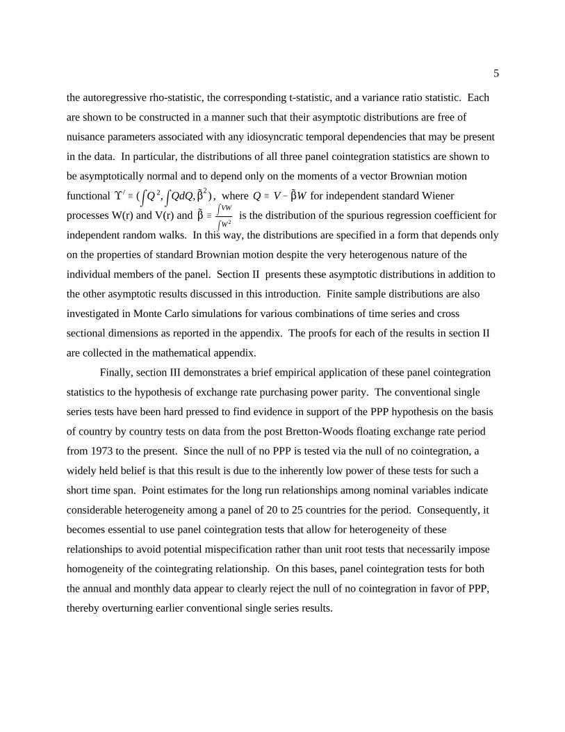
the autoregressive rho-statistic, the corresponding t-statistic, and a variance ratio statistic. Each

are shown to be constructed in a manner such that their asymptotic distributions are free of

nuisance parameters associated with any idiosyncratic temporal dependencies that may be present

in the data. In particular, the distributions of all three panel cointegration statistics are shown to

be asymptotically normal and to depend only on the moments of a vector Brownian motion

functional , where for independent standard Wiener

processes W(r) and V(r) and is the distribution of the spurious regression coefficient for

independent random walks. In this way, the distributions are specified in a form that depends only

on the properties of standard Brownian motion despite the very heterogenous nature of the

individual members of the panel. Section II presents these asymptotic distributions in addition to

the other asymptotic results discussed in this introduction. Finite sample distributions are also

investigated in Monte Carlo simulations for various combinations of time series and cross

sectional dimensions as reported in the appendix. The proofs for each of the results in section II

are collected in the mathematical appendix.

Finally, section III demonstrates a brief empirical application of these panel cointegration

statistics to the hypothesis of exchange rate purchasing power parity. The conventional single

series tests have been hard pressed to find evidence in support of the PPP hypothesis on the basis

of country by country tests on data from the post Bretton-Woods floating exchange rate period

from 1973 to the present. Since the null of no PPP is tested via the null of no cointegration, a

widely held belief is that this result is due to the inherently low power of these tests for such a

short time span. Point estimates for the long run relationships among nominal variables indicate

considerable heterogeneity among a panel of 20 to 25 countries for the period. Consequently, it

becomes essential to use panel cointegration tests that allow for heterogeneity of these

relationships to avoid potential mispecification rather than unit root tests that necessarily impose

homogeneity of the cointegrating relationship. On this bases, panel cointegration tests for both

the annual and monthly data appear to clearly reject the null of no cointegration in favor of PPP,

thereby overturning earlier conventional single series results.

yit ' Xit$ % eit

yit ' " % Xit$ % eit

yit ' " % *t % Xit$ % eit

",$,*

6

(1)

(1')

(1'')

II. Asymptotic Properties of Panel Regressions for Integrated Regressors

2.1 The Panel Models and Basic Methodology

We will in general refer to two sets of panel regression models. The first we will refer to as

homogenous, reflecting the notion that the individual cross sections of the panels are assumed to

share common long run features under the alternate hypothesis of cointegration, including

common cointegrating vector coefficients, means, or deterministic time trends when applicable.

Thus, we will write these type of regressions as

Model 1 (homogeneous panel):

for which the variables y and X are subscripted by the index i to indicate that they exist for each of

i = 1, ... , N different cross sections. The parameters on the other hand, are not subscripted

by the index i to indicate that they will be assumed to be homogenous across individual cross

sections of the panel under the alternate hypothesis that they reflect the coefficients of a

cointegrating relationship. By comparison, we will refer to the second set of models as

heterogenous, reflecting the fact that the individual cross sections for these panels are not

necessarily assumed to be homogenous under the alternate hypothesis. Thus, we will write these

type of regressions as

yit ' Xit$i % eit

yit ' "i % Xit$i % eit

yit ' "i % *i t % Xit$i % eit

yit ' *t % "i % Xit$i % eit

",$,*

Zi

Zi / ( yi , Xi)) Zi

7

(2)

(2')

(2'')

(3)

Model 2 (heterogenous panel):

for which the coefficients are now subscripted with the cross sectional index i. The

distinction between these two types of models is critical in terms of the type of alternate

hypotheses that they will permit under cointegration testing. For the first set, the alternate to no

cointegration must be that if the individual are cointegrated, then they will exhibit the same long

run cointegrating relationships. For the second, the alternate to no cointegration may be that the

individual cross sections contain cointegrating relationships that are free to take on different

values for different members of the panel.

Of course models need not be restricted to exclusively homogenous or heterogeneous long

run parameters. In some cases one may also wish to consider hybrid models which retain some

features of both model types (1) and (2). For example, the model given by

Model 3 (hybrid, with common time dummies):

can be useful if one wishes to permit common aggregate shocks that are shared across individuals

while still allowing for both dynamic and long run idiosyncratic responses.

In each model, unless otherwise indicated, all other assumptions regarding the properties

of the stochastic processes will be the same. Specifically, let be defined by the vector

. Then we will assume that each individual is generated by the process

Zio

Si / limT64 E T &1(jT

t'1>it) (j

T

t'1>)it)

Zit ' Zit&1 % >it

>it / (>yit ,>

xit)

) 1

Tj[Tr]

t'1>it 6 Bi(Si)

T64 Bi(Si)

r, [0,1] Si

Si

Si / Soi % 'i % ')

i Soi

>it 'i

>it

Si T21 i , T)

21 i

Xit Si

",*,$

8

We will also assume for convenience that initial conditions are given by constant to3

avoid complications from possible covariation of the initial condition with subsequent errors,which is considered in Quah (1994).

See standard references, eg. Phillips (1986,1987), Phillips and Durlauf (1986), for further4

discussion of the conditions under which assumption 1.1 holds more generally.

(4)

, for which the following standard assumption holds for each individual cross3

section:

Assumption 1.1 (invariance principle): The process satisfies ,

as , where -> signifies weak convergence, and is vector Brownian motion defined

over the real interval , with asymptotic covariance .

Thus, assumption 1.1 is simply a statement that the standard functional central limit theorem is

assumed to hold individually for each cross sectional series as T grows large. The conditions on

the error process required for this convergence are relatively weak and includes the entire class of

stationary ARMA processes. The asymptotic covariance matrix is given by4

which can be decomposed as where is the contemporaneous covariance

among the components of for a given cross section i, and captures the dynamic covariances

among the components of for a given cross section i. The off diagonal terms of the asymptotic

covariance matrix , denoted , thus capture the idiosyncratic endogenous feedback

among the I(1) variables, and in keeping with the cointegration literature we do not require that

the regressors be exogenous. The fact that is permitted to vary across individual sections

of the panel reflects the fact that in general we will permit all dynamics that are absorbed in the

asymptotic covariance matrix to be heterogeneous for any of the models (1) through (3),

regardless of whether or not the long run parameters are treated as varying across individual

sections.

Si / Soi % 'i % ')

i

where Soi / T &1j

T

t'1

>it>)

it , 'i / T &1jki

s'1

ws kijT

t'1

>it>)

it&s

Si

'i

wsk >it Zit ' Di Zi t&1 % >it

wsk i' 1& s

k i% 1

>it Si

E [>it ,>jt]' 0 forall i…j

IN q Si > 0

9

(5)

A number of consistent estimators are available for the individual , typically based on

kernel estimators for the component. Typical estimators take the form

for some lag window , where is obtained from an autoregression

individually for each i. A commonly used lag window is based on the Newey-West estimator with

. More recently, Andrews and Monahan (1992), Lee and Phillips (1994) and

Levin and den Haan (1995) have proposed robust asymptotic covariance estimators based on

prewhitening of the residuals to improve finite sample estimates of . Based on the

preliminary investigations of Park and Ogaki (1991) for these type of estimators in the context of

standard cointegrating regressions, the finite sample improvements from these prewhitening

procedure may be particular attractive in the present context of panel cointegration tests with

relatively small time series dimensions.

In addition to the conditions for the invariance principle with regard to the time series

dimension, we will also assume the following condition in keeping with a panel data approach

Assumption 1.2 (cross sectional independence): The individual processes are assumed to be

independent cross sectionally, so that . More generally, the asymptotic

covariance matrix for a panel of size NxT is given as , which is block diagonal

positive semidefinite with the ith diagonal block given by the asymptotic covariances for cross

section i.

Formally, this condition will be required to apply standard central limit theorems in the cross

sectional dimension in the presence of heterogenous errors. In practice, the assumption is not as

restrictive as it may first appear given the possibility of incorporating aspects of the hybrid models

of type (3) to capture any disturbances that are common across members of the panel as is

T &2 jT

t' 1

Zit&1 Z )

it&1 6 S1/2i m

1

0Zi(r)Zi(r))drS1/2

i

T &1 jT

t' 1

Zit&1>)

it 6 S1/2i m

1

0Zi(r) dZi(r))drS1/2

i % 'i

Zi(r) / ( Vi(r) , Wi(r) ))

Si

Zi(r)

Zi(r)

10

In contrast to the common time dummies, the presence of stochastic cointegrating5

relationship among cross sections will generally impact the limiting distributions if not properlyaccommodated.

(6a)

(6b)

frequently done for panels. On the other hand, the condition that the covariance matrix for the

panel as a whole be positive semidefinite rules out any singularities that would reflect potential

intra-panel stochastic cointegrating relationships. 5

Together, conditions 1.1 and 1.2 regarding the time series and cross sectional properties

of the error processes for the time series panel will provide us with the basic methodology for

investigating the asymptotic properties of various statistics as both N and T grow large. Thus, the

first assumption will allow us to make use of standard convergency results regarding asymptotics

in the time series dimension for each of the individual cross sections. In particular, we will make

use of the fact that the following convergencies, developed in Phillips and Durlauf (1986) and

Park and Phillips (1988), must also hold for each of the individual cross sections i as T grows

large, so that

where is a vector Brownian motion such that V(r) and W(r) are

independent standard Wiener processes, and and its components are defined as in (4) above.

The decomposition that is implicit in these convergencies, in terms of the transformation of

discrete statistics that are heterogenous across i to continuous statistics that are expressed as a

product of standard Brownian motion and the idiosyncratic asymptotic covariance terms, is key in

permitting the use of panel data methods effectively to variables with such general and

heterogenous error processes. In particular, the fact that the elements of are standard

implies that the distributions of functionals of will be identical across individual i so that

more standard central limit theorems can be applied to sums of these standardized Brownian

eit

$NT

$

$iT

$i

$iT

$NT

$NT

eit ~ I(1)

Si ' S

$NT ~ Op( N &1/2 ) $NT plimN,T64 $NT ' 0

t$NT~ Op( T 1/2 ) t$NT

N,T64

$NT

$iT Op(1)

",*,$

11

motion functionals as N grows large. In this case the resulting distributions will be asymptotically

normal and free of nuisance parameters with moments determined solely by the properties of the

Brownian motion functionals, as we will see.

2.2 Asymptotic Properties of Spurious Regressions in Panels

In order to facilitate analysis of the asymptotic properties of residual stationarity based tests, we

first investigate a number of interesting properties of panel regressions based on models (1) and

(2) for the case in which the residual process is integrated of order one so that the regressions

can be characterized as "spurious" in the long run for each individual cross section. Define as

the pooled panel OLS estimator of the spurious regression slope coefficient for models of type

(1), and let refer to individual equation OLS estimator of the spurious regression slope

coefficients in models of type (2), or a hybrid model such as (3). Clearly, the asymptotic

properties of the estimator will not differ from the standard results for single series spurious

regressions. In contrast, the asymptotic properties of the estimator for models of type (1) can

differ markedly. In particular, for the estimator we have the following proposition.

Proposition 2.1 (Spurious Regressions for Homogeneous Panels): If for all i, then

for all models (1) with homogenous coefficients and ,

(a). so that is a consistent estimator in the sense that .

(b). so that diverges as .

The consistency result for is in contrast to the classical spurious regression case of the single

equation OLS estimators , which are nonconvergent as in Phillips (1986). Not

surprisingly, the distinction is of fundamental importance for the properties of residual stationarity

tests for cointegration that are based on estimates of the long run parameters associated

with models (1) and (2) as we will see in the next subsection. First, however, it is worthwhile to

note several more immediate implications of proposition 3.1 for spurious regressions in panels.

Notice for example that cross sectional asymptotics is not in itself sufficient to remedy the

spurious regression problem in the sense that standard t-statistic will continue to diverge as N and

N jN

i'1j

T

t'1

L &222 i x 2

it

&1

jN

i'1j

T

t'1

(L11 iL22 i)&1 xityit&

L21 i

L11 i

x 2it 6 N( 0 , 2/3)

$NT t$NT

Si

Li Si

N,T64

$NT t$NT

$NT L21 i ' 0

$NT

Si ' S T21 ' 0 N,T643

2N $NT 6 N(0,

T11

T22

)

T &1/2 t$NT6 N( 0,2/3)

12

T grow large. Thus, a researcher who chooses to ignore the unit root properties of the variables

of a panel will still face the problem of falsely inferring a significant relationship among integrated

variables with certainty as the time series dimension grows large in the absence of cointegration

even as the cross sectional dimension grows large. Furthermore, the standardized asymptotic

distributions of both and will in general be contaminated by data dependencies

associated with dynamics reflected in the nuisance parameters of the long run covariance matrix

. However, the following general result does provide some insights regarding the conditions

under which this data dependency does not pertain for certain special case distributions.

Lemma 2.1 Let be the lower triangular Cholesky decomposition of . Then under the

conditions of proposition 2.1, the convergence

holds as .

Indirectly, this lemma illustrates the precise nature of the nuisance parameter dependencies for

estimators such as and . In particular, the left hand side of the expression more closely

resembles the panel OLS estimator in the event that , which corresponds to the case

of strict exogeneity for the regressors. When the dynamics are also assumed to be homogeneous

across individual sections so that the elements of L are no longer indexed by i, then the following

special case results are obtained.

Proposition 2.2 (Special Case Distributions of ): If the dynamics associated with the serial

correlation patterns for all models (1) are also homogenous and the regressors are strictly

exogenous, so that for all i with , then as

(a).

(b).

DNT & 1 / jN

i'1j

T

t'1e 2

it&1

&1

jN

i'1j

T

t'1eit&1)eit & 8i

Si ' Li L)

i ' So

T11,T22

N $NT t$NT

$NT

t$NT

DNT

13

(7)

In the event that the disturbances are i.i.d. so that , then the asymptotic variances

of part (a) are replaced by the more standard sample variance and part (b) continues to

hold as is. In fact, these special cases correspond to the more restrictive assumptions that have

commonly been used in more traditional panel data regressions. Table B.I of the appendix reports

the results of Monte Carlo simulations for the finite sample distributions of and

respectively for various combinations of N and T for 10,000 draws of independent random walks

under the null spurious with no estimated constants and also for the case in which homogenous

constants are estimated. The tables demonstrate that in this case the asymptotic distributions are

very well approximated even for relatively small samples, and that furthermore the invariance to

the estimation of homogenous constants holds well in relatively small samples.

In general however, it should be clear that these assumptions are likely to be overly

restrictive for most of the purposes to which one would like to use cointegration tests. Of course

in principle one might imagine constructing a feasible statistic free of nuisance parameters even in

the most general case on the basis of the relationships in lemma 2.1. But lemma 2.1 clearly

indicates that the feasible statistic would in general not be a simple transformation of either

or . Instead, as we shall see in the next subsections, transformations based on residual

stationarity tests will provide more straightforward feasible statistics. Furthermore, in contrast to

statistics based on lemma 2.1, statistics based on estimated residuals can be made to

accommodate models such as (2) that also include heterogenous long run parameters.

2.3 Asymptotic Properties of Cointegration Tests in Panels

In this subsection we consider the asymptotic properties and distributions of test statistics for

cointegration based on estimated residuals of the spurious regressions of models (1) through (3).

We will consider both residual based stationarity tests as well as residual based variance ratio

tests. In particular, for the latter, define the panel autoregressive coefficient estimator as

eit 8i

eit ' Deit&1 % µ it 8i ' T &1jki

s'1ws kij

T

t'1µ itµ it&s

wsk i8i 'i

eit Zit DNT

8i

eit ~ I(1)

eit

T N(DNT&1) 6 N(0,2) N,T64 Si ' S >0

NT(T&1) (DNT&1) 6 N(0,2) N64

tDNT6 N(0,1) N64 N,T64

Si ' S >0

14

under the null of nonstationarity for the residuals , where is based on the estimated residuals

of the autoregression such that for some lag window

, so that is a scalar analogous to defined in (5) above, in that it is based on

autoregressions of the scalar time series rather than the vector time series . Thus, can

be thought of as a pooled version of the unstandardized Phillips and Perron statistic. The

nonparametric estimation of is not critical for the first two result, though, as they will hold

equally well for parametric unit root tests constructed along the lines of the Augmented Dickey-

Fuller statistic. The first result is a direct consequence of proposition 2.1 for spurious regressions.

Proposition 3.1 (Asymptotic Equivalency Results): If for all i, then

(a). The distribution of residual stationarity tests in all models (1) with homogeneous

coefficients are invariant to whether the residuals are known or are estimated.

(b). The same is not true for models of type (2) and (3) with heterogeneous coefficients.

Thus part (a) provides a type of superconsistency result that operates even in the absence of

cointegration for certain panels as N grows large. As a consequence, tests of cointegration for

homogenous panels of model type (1) will have the same critical values for large N as raw unit

root tests applied to similarly dimensioned panels. The following result derives then as a direct

corollary to proposition 3.1.

Corollary 3.1 (Special Case Asymptotic Distributions for Homogenous Panels): Panel unit

root tests applied to the estimated residuals of models (1), (1'), or (1'') with homogenous

coefficients will be distributed as follows under the null of no cointegration.

(a). as for general disturbances.

(b). as for i.i.d. disturbances, regardless of T.

(c). as for i.i.d. disturbances, regardless of T, and as for general

disturbances.

Part (a) of the corollary is in fact the distribution that is obtained by Levin and Lin (1994) for

NT(T&1) (D&1)

N64

T N (D&1) NT(T&1) (D&1) tD&1

$NT

tD&1

15

For example if we compare these tables to similar tables reported for panel unit root6

simulations in Levin and Lin (1994), or Pedroni (1993) for for various N andT.

simple unit root tests in panels. Result (b) is a special case asymptotic distribution that holds

regardless of the time series dimension T, so that under certain conditions cointegration tests can

be performed even for panels with extremely small time series dimensions such as T=5. Clearly,

this result can also be expected to hold for the case in which there exists some degree of serial

correlation as long as it is homogenous across the individual cross sections i, and of low order

relative to the T, since in this case the dynamics could also be estimated parametrically as .

What is perhaps more interesting, however, is that appropriate standardization for the distribution

of the corresponding t-statistic in part (c) is the same for the two cases. In fact this result helps to

explain why Monte Carlo studies for panel unit root tests such as reported in Levin and Lin

indicate very close approximations to the asymptotic distributions even for very small T. The

answer appears to be that for the special case i.i.d. random walks that are used in the simulations,

the time series dimension is in fact not relevant as N grows sufficiently large.

Table B.II reports the results of Monte Carlo simulations for the finite sample distributions

of the three statistics , and of corollary 3.1 for various

combinations of N and T for 10,000 draws of independent random walks under the null spurious

with no estimated constants, as well as the case in which homogenous constants are estimated.

The tables reflect the fact that although the distribution of the residual stationarity test applied to

estimated residuals is asymptotically equivalent to the case in which the residuals are known, for

finite samples the critical values will not be identical. Specifically, in the case of cointegration6

testing, the asymptotic distribution additionally depends on converging to zero as N grows

large, so that the residual stationarity tests do not reach their asymptotic distributions as quickly

for finite N. Still, the asymptotic distributions are fairly well approximated, particularly in the

case of the t-statistic, as N grows large even for small T. For example, in a Monte Carlo

simulation for N=200, T=10, the mean and variance were calculated to be -0.02 and 1.00

respectively for the case of with no constant.

In any case, it is important to keep in mind that although they can be very convenient

ZvNT/ j

N

i'1j

T

t'1L

&211 i e 2

it&1

&1

ZDNT/ j

N

i'1j

T

t'1L

&211 i e 2

it&1

&1

jN

i'1j

T

t'1L

&211 i (eit&1 eit & 8i)

ZtDNT

/ F2NT j

N

i'1j

T

t'1L

&211 i e 2

it&1

&1/2

jN

i'1j

T

t'1L

&211 i (eit&1)eit & 8i)

FNT / 1

N jN

i'1(L11 iFi)

2 8i '1

2(F2

i & s 2i ) s 2

i / T &1jT

t'1µ2

it Li

Si 1, R

K) / (mQ 2,mQdQ, $2) $ / mVW

mW2Q / V& $W R(i)

R

16

under the appropriate circumstances, the results of corollary 3.1 should be used only in the special

case of model (1), for which the alternate hypothesis of cointegration requires that the

cointegrating relationships are also identical for each cross section. While some applications may

fit this description, more generally one should expect the alternate hypothesis to be such that

models of type (2) or (3) must be employed, since the alternate to no cointegration is likely to be

that any one of a number of different and unknown cointegrating relationships hold for the

individual members of the panel. In this case the asymptotic distributions for cointegration tests

will differ substantially from the raw unit root tests. Furthermore, it becomes important in the

general case for heterogenous panels to take account of the idiosyncratic feedback effect among

variables. In particularly, we obtain the following very general result, which includes the case of

heterogenous panels.

Proposition 3.2 (Asymptotic Distributions of Residual Tests of Cointegration in Heterogenous

Panels): Based on the estimated residuals of Models (2), define the following statistics.

where , , and is based on consistent

estimation of . Let signify the mean and variance for the vector Brownian motion

functional , where , and , i = 1,2,3 refers to

the i x i

upper sub-matrix of . Then the asymptotic distributions of these statistics are free of any

ZtNT& 12 (11(1%13))

&1/2 N 6 N (0, N)

(3)R(3)N(3) )

T N (ZDNT& 1) & 121

&11 N 6 N (0, N)

(2)R(2)N(2) )

TN 3/2 ZvNT& 1&1

1 N 6 N (0, N)

(1)R(1)N(1) )

Si N,T64

N)

(1) ' & 1&21 N)

(2) ' & (1&11 ,121

&21 )

N)

(3) ' (1&1/21 (1%13)

&1/2, & 1

2121

&3/21 (1%13)

&1/2, & 1

2121

&1/21 (1%13)

&3/2 )

Li Si

L22 i ' T22 i L211 i ' T11 i &

T221 i

T22 i

L 211 i

L 211 i

1 , R

17

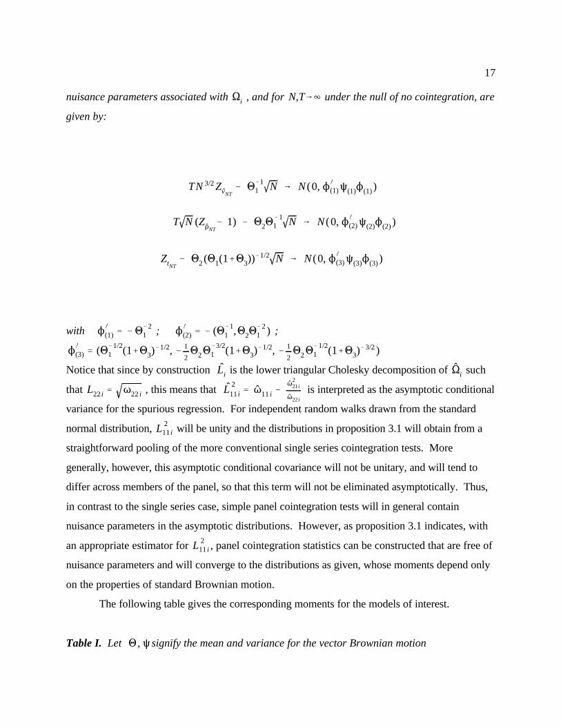
nuisance parameters associated with , and for under the null of no cointegration, are

given by:

with ; ;

Notice that since by construction is the lower triangular Cholesky decomposition of such

that , this means that is interpreted as the asymptotic conditional

variance for the spurious regression. For independent random walks drawn from the standard

normal distribution, will be unity and the distributions in proposition 3.1 will obtain from a

straightforward pooling of the more conventional single series cointegration tests. More

generally, however, this asymptotic conditional covariance will not be unitary, and will tend to

differ across members of the panel, so that this term will not be eliminated asymptotically. Thus,

in contrast to the single series case, simple panel cointegration tests will in general contain

nuisance parameters in the asymptotic distributions. However, as proposition 3.1 indicates, with

an appropriate estimator for , panel cointegration statistics can be constructed that are free of

nuisance parameters and will converge to the distributions as given, whose moments depend only

on the properties of standard Brownian motion.

The following table gives the corresponding moments for the models of interest.

Table I. Let signify the mean and variance for the vector Brownian motion

K) / (mQ 2,mQdQ, $2) $ / mVW

mW2Q / V& $W 1) , R)

1)) , R))

V ),W ) V )),W ))

1 '

0.250

&0.693

0.889

R'

0.110

&0.011 0.788

0.243 &1.326 3.174

1)'

0.116

&0.698

0.397

R)'

0.011

&0.013 0.179

0.026 &0.238 0.480

1))'

0.056

&0.590

0.182R)) '

0.001

&0.001 0.034

0.003 &0.042 0.085

ZvNT, Z )

vNT, Z ))

vNT

N64

TN 3/2 ZvNT& 4.00 N 6 N (0, 27.81)

TN 3/2 Z )

vNT& 8.62 N 6 N (0, 60.75)

18

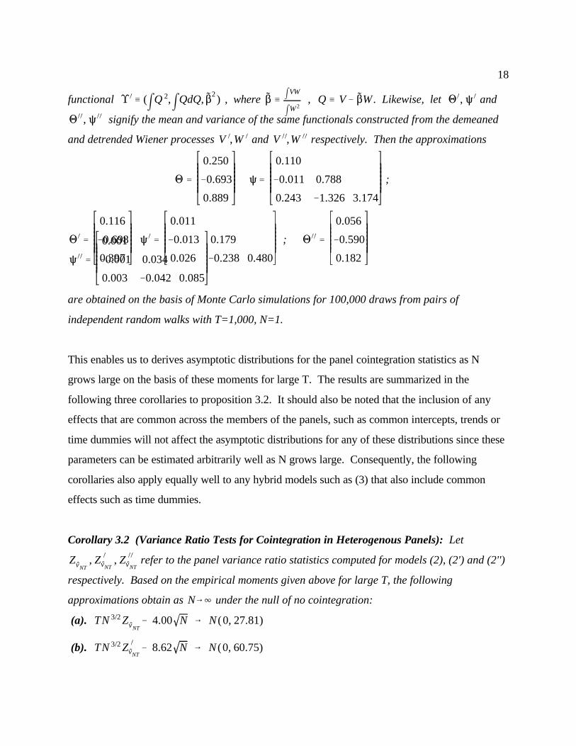
functional , where , . Likewise, let and

signify the mean and variance of the same functionals constructed from the demeaned

and detrended Wiener processes and respectively. Then the approximations

;

;

are obtained on the basis of Monte Carlo simulations for 100,000 draws from pairs of

independent random walks with T=1,000, N=1.

This enables us to derives asymptotic distributions for the panel cointegration statistics as N

grows large on the basis of these moments for large T. The results are summarized in the

following three corollaries to proposition 3.2. It should also be noted that the inclusion of any

effects that are common across the members of the panels, such as common intercepts, trends or

time dummies will not affect the asymptotic distributions for any of these distributions since these

parameters can be estimated arbitrarily well as N grows large. Consequently, the following

corollaries also apply equally well to any hybrid models such as (3) that also include common

effects such as time dummies.

Corollary 3.2 (Variance Ratio Tests for Cointegration in Heterogenous Panels): Let

refer to the panel variance ratio statistics computed for models (2), (2') and (2'')

respectively. Based on the empirical moments given above for large T, the following

approximations obtain as under the null of no cointegration:

(a).

(b).

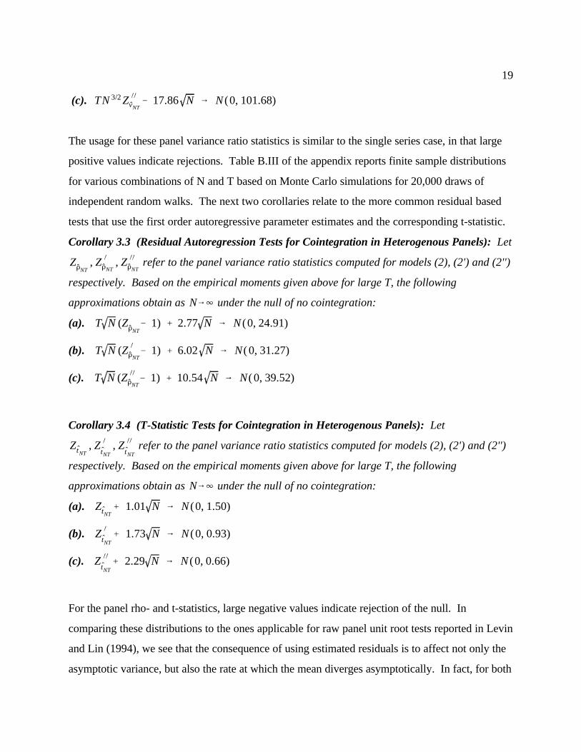
TN 3/2 Z ))

vNT& 17.86 N 6 N (0, 101.68)

ZDNT, Z )

DNT, Z ))

DNT

N64

T N (ZDNT& 1) % 2.77 N 6 N (0, 24.91)

T N (Z )

DNT& 1) % 6.02 N 6 N( 0, 31.27)

T N (Z ))

DNT& 1) % 10.54 N 6 N( 0, 39.52)

ZtNT, Z )

tNT, Z ))

tNT

N64

ZtNT% 1.01 N 6 N (0, 1.50)

Z )

tNT% 1.73 N 6 N (0, 0.93)

Z ))

tNT% 2.29 N 6 N (0, 0.66)

19

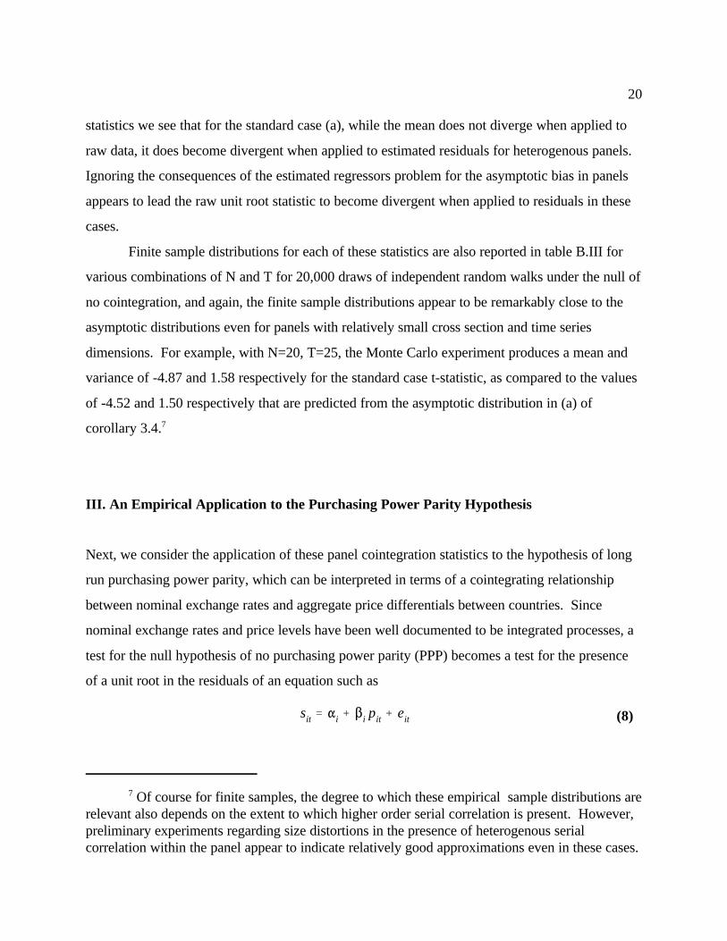
(c).

The usage for these panel variance ratio statistics is similar to the single series case, in that large

positive values indicate rejections. Table B.III of the appendix reports finite sample distributions

for various combinations of N and T based on Monte Carlo simulations for 20,000 draws of

independent random walks. The next two corollaries relate to the more common residual based

tests that use the first order autoregressive parameter estimates and the corresponding t-statistic.

Corollary 3.3 (Residual Autoregression Tests for Cointegration in Heterogenous Panels): Let

refer to the panel variance ratio statistics computed for models (2), (2') and (2'')

respectively. Based on the empirical moments given above for large T, the following

approximations obtain as under the null of no cointegration:

(a).

(b).

(c).

Corollary 3.4 (T-Statistic Tests for Cointegration in Heterogenous Panels): Let

refer to the panel variance ratio statistics computed for models (2), (2') and (2'')

respectively. Based on the empirical moments given above for large T, the following

approximations obtain as under the null of no cointegration:

(a).

(b).

(c).

For the panel rho- and t-statistics, large negative values indicate rejection of the null. In

comparing these distributions to the ones applicable for raw panel unit root tests reported in Levin

and Lin (1994), we see that the consequence of using estimated residuals is to affect not only the

asymptotic variance, but also the rate at which the mean diverges asymptotically. In fact, for both

sit ' "i % $i pit % eit

20

Of course for finite samples, the degree to which these empirical sample distributions are7

relevant also depends on the extent to which higher order serial correlation is present. However,preliminary experiments regarding size distortions in the presence of heterogenous serialcorrelation within the panel appear to indicate relatively good approximations even in these cases.

(8)

statistics we see that for the standard case (a), while the mean does not diverge when applied to

raw data, it does become divergent when applied to estimated residuals for heterogenous panels.

Ignoring the consequences of the estimated regressors problem for the asymptotic bias in panels

appears to lead the raw unit root statistic to become divergent when applied to residuals in these

cases.

Finite sample distributions for each of these statistics are also reported in table B.III for

various combinations of N and T for 20,000 draws of independent random walks under the null of

no cointegration, and again, the finite sample distributions appear to be remarkably close to the

asymptotic distributions even for panels with relatively small cross section and time series

dimensions. For example, with N=20, T=25, the Monte Carlo experiment produces a mean and

variance of -4.87 and 1.58 respectively for the standard case t-statistic, as compared to the values

of -4.52 and 1.50 respectively that are predicted from the asymptotic distribution in (a) of

corollary 3.4. 7

III. An Empirical Application to the Purchasing Power Parity Hypothesis

Next, we consider the application of these panel cointegration statistics to the hypothesis of long

run purchasing power parity, which can be interpreted in terms of a cointegrating relationship

between nominal exchange rates and aggregate price differentials between countries. Since

nominal exchange rates and price levels have been well documented to be integrated processes, a

test for the null hypothesis of no purchasing power parity (PPP) becomes a test for the presence

of a unit root in the residuals of an equation such as

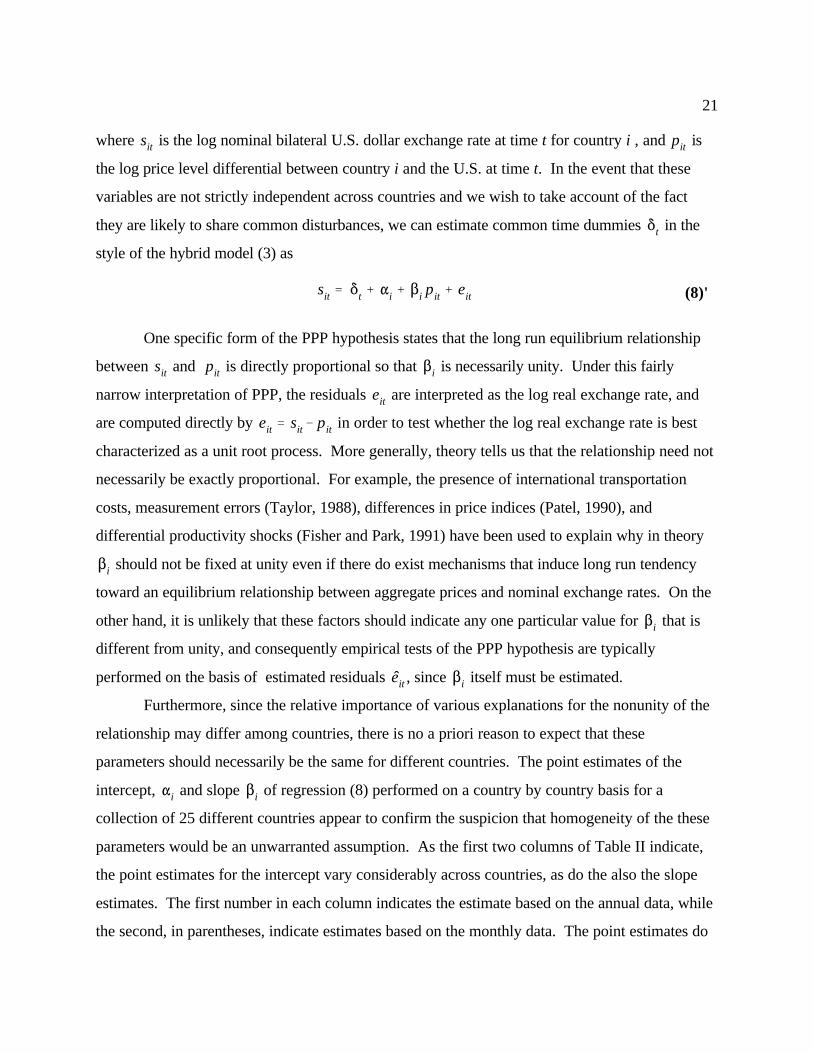
sit ' *t % "i % $i pit % eit

sit pit

*t

sit pit $i

eit

eit ' sit& pit

$i

$i

eit $i

"i $i

21

(8)'

where is the log nominal bilateral U.S. dollar exchange rate at time t for country i , and is

the log price level differential between country i and the U.S. at time t. In the event that these

variables are not strictly independent across countries and we wish to take account of the fact

they are likely to share common disturbances, we can estimate common time dummies in the

style of the hybrid model (3) as

One specific form of the PPP hypothesis states that the long run equilibrium relationship

between and is directly proportional so that is necessarily unity. Under this fairly

narrow interpretation of PPP, the residuals are interpreted as the log real exchange rate, and

are computed directly by in order to test whether the log real exchange rate is best

characterized as a unit root process. More generally, theory tells us that the relationship need not

necessarily be exactly proportional. For example, the presence of international transportation

costs, measurement errors (Taylor, 1988), differences in price indices (Patel, 1990), and

differential productivity shocks (Fisher and Park, 1991) have been used to explain why in theory

should not be fixed at unity even if there do exist mechanisms that induce long run tendency

toward an equilibrium relationship between aggregate prices and nominal exchange rates. On the

other hand, it is unlikely that these factors should indicate any one particular value for that is

different from unity, and consequently empirical tests of the PPP hypothesis are typically

performed on the basis of estimated residuals , since itself must be estimated.

Furthermore, since the relative importance of various explanations for the nonunity of the

relationship may differ among countries, there is no a priori reason to expect that these

parameters should necessarily be the same for different countries. The point estimates of the

intercept, and slope of regression (8) performed on a country by country basis for a

collection of 25 different countries appear to confirm the suspicion that homogeneity of the these

parameters would be an unwarranted assumption. As the first two columns of Table II indicate,

the point estimates for the intercept vary considerably across countries, as do the also the slope

estimates. The first number in each column indicates the estimate based on the annual data, while

the second, in parentheses, indicate estimates based on the monthly data. The point estimates do

"i (intercept $i (slope) TN 3/2 Z vNTT N(ZDNT

& 1) ZtNTZ tNT

Ki (lags

sit ' "i % $i pit % eit sitpit

22

not differ much between the annual and monthly data in most cases, but they do vary considerably

among countries, with point estimates for the slope varying between 0.15 (0.48) for Belgium and

2.26 (2.12) for India, and 1.81 (1.85) for Japan. The intercepts vary even more, from -7.21

(-7.22) for Italy, and 1.31 (1.45) for Mexico, and 0.53 (0.53) for the U.K. For these reasons, the

null of no PPP is best tested on the basis of the absence of a cointegrating relationship rather than

on the basis of a raw unit root test. Furthermore, without strong evidence to the contrary, the

corresponding parameters of the spurious regression must be allowed to vary across countries if Table II. Purchasing power parity estimates of individual country slopes and intercepts andindividual cointegration statistics compared to heterogeneous panel cointegration statistics forthe null of no PPP. Annual, T=20, and monthly, T=246, IFS data, June 1973 to Dec. 1994.

Country (PP) (ADF)

Belgium -3.63 (-3.66) 0.15 (0.48) 6.86 (9.29) -6.32 (-6.20) -1.78 (-1.77) -1.93 (-1.49) 1 (16)

Denmark -1.97 (-2.01) 1.21 (1.43) 10.57 (12.12) -6.48 (-6.61) -1.82 (-1.82) -1.79 (-1.68) 1 (13)

France -1.90 (-1.92) 1.72 (1.71) 5.41 (14.71) -7.40 (-7.75) -1.96 (-1.97) -2.02 (-2.16) 1 (6)

Germany -0.67 (-0.70) 0.74 (0.70) 12.31 (15.09) -7.07 (-7.91) -1.91 (-2.00) -1.88 (-1.77) 1 (17)

Ireland 0.35 ( --- ) 0.74 ( --- ) 6.88 ( --- ) -7.98 ( --- ) -2.05 ( --- ) -2.18 ( --- ) 1 ( - )

Italy -7.21 (-7.22) 0.80 (0.88) 6.64 (13.72) -8.05 (-7.53) -2.03 (-1.94) -1.96 (-1.62) 1 (11)

Netherland -0.79 (-0.82) 0.68 (0.69) 12.48 (15.38) -7.28 (-7.74) -1.94 (-1.96) -1.94 (-1.88) 1 (20)

Sweden -1.81 (-1.80) 1.15 (1.24) 11.18 (12.86) -6.32 (-6.56) -1.77 (-1.80) -1.83 (-1.57) 1 (20)

Switzerland -0.51 (-0.54) 0.98 (1.16) 14.21 (17.42) -8.43 (-9.21) -2.12 (-2.14) -2.13 (-2.09) 1 (17)

U.K. 0.53 (0.53) 0.57 (0.68) 16.18 (20.23) -9.75 (-10.17) -2.31 (-2.26) * -3.36 (-2.38) 3 (21)

Canada -0.20 (-0.20) 1.10 (1.42) 9.71 (9.05) -7.30 (-6.11) -2.03 (-1.72) -2.51 (-1.62) 1 (16)

Japan -5.14 (-5.19) 1.81 (1.85) 11.59 (13.75) -9.68 (-8.93) -2.33 (-2.12) -2.22 (-1.81) 1 (18)

Greece -4.60 (-4.57) 1.01 (1.03) 4.10 (12.21) -6.24 (-6.59) -1.76 (-1.81) -2.87 (-1.88) 3 (14)

Iceland -3.50 ( --- ) 0.99 ( --- ) 6.87 ( --- ) -7.75 ( --- ) -2.02 ( --- ) -2.37 ( --- ) 3 ( - )

Portugal -4.79 (-4.77) 0.96 (1.02) 5.04 (9.49) -5.39 (-4.84) -1.69 (-1.53) -2.73 (-1.60) 5 (16)

Spain -4.74 (-4.74) 0.80 (0.86) 11.80 (12.27) -6.66 (-6.17) -1.83 (-1.75) -2.04 (-1.50) 1 (16)

Turkey -6.07 (-5.93) 1.11 (1.09) 7.55 (9.64) -4.73 (-4.12) -1.45 (-1.29) -1.79 (-1.87) 3 (15)

Australia -0.10 ( --- ) 1.43 ( --- ) 12.26 ( --- ) -8.12 ( --- ) -2.03 ( --- ) -1.98 ( --- ) 1 ( - )

N. Zealand -0.42 (-0.38) 0.84 (1.19) 10.27 (21.26) -8.56 (-11.18) -2.14 (-2.36) -2.14 (-2.75) 1 (18)

S. Africa -0.42 ( --- ) 1.14 ( --- ) 5.47 ( --- ) -7.87 ( --- ) -2.05 ( --- ) -3.08 ( --- ) 3 ( - )

Chile -4.94 (-4.84) 1.11 (1.18) 7.86 * (37.73) -9.41 * (-50.19) -2.68 * (-5.51) -1.62 (-2.26) 1 (21)

Mexico 1.31 (1.45) 1.03 (1.04) 5.32 (18.87) -9.73 (-9.57) -2.33 (-2.06) -2.10 (-2.61) 1 (10)

India -2.42 (-2.37) 2.26 (2.12) 5.72 (5.04) -12.93 (-8.62) * -4.06 (-2.24) -2.41 (-1.90) 1 (6)

Korea -6.57 (-6.56) 1.08 (0.98) 10.61 (8.54) -7.88 (-5.12) -2.06 (-1.68) -2.77 (-1.45) 5 (6)

Pakistan -2.62 ( --- ) 3.03 ( --- ) 2.50 ( --- ) -4.88 ( --- ) -1.61 ( --- ) -2.14 ( --- ) 4 ( - )

Pooled (20) 35.93 * (54.37) * -34.61 * (-34.90) * -9.41 * (-8.95) * -9.36 (-8.09) Pooled (25) 35.14 * -37.87 * -10.27 * -10.74

Notes: Estimated equation is (8): , where is the log nominal bilateral U.S. dollarexchange rate at time t for country i , and is the log price level differential between country i and the U.S. at timet. Estimates for monthly data are in parentheses. Pooled (20) excludes those countries for which monthly data isunavailable or incomplete over the chosen time span. An asterisk indicates rejections at the 10% level or better.

sit pit

23

Raw unit root tests were also performed on and to confirm their nonstationarity.8

they are to be pooled for the purposes of a panel cointegration test to avoid misspecification

from a false homogeneity restriction.

Typically, cointegration tests of the PPP hypothesis have been conducted on a single

country by country basis. For the most part, however, tests conducted on a single country basis

have been largely unable to reject the null of no PPP for the post Bretton Woods period of

floating exchange rates. Studies of this type include for example Taylor (1988), Corbai and

Ouliaris (1988), Baillie and Selover (1987) and Patel (1990), to name only a few. On the other

hand, studies that employ data spanning much longer time frames, based on Lee's (1976) annual

exchange rate and CPI data from 1900 to 1973 combined with post Bretton Woods IFS data,

generally do reject the null of no PPP. This leaves open the question of whether the failure to

reject the null in the post 1973 data alone is due to an inherent regime change that no longer

favors PPP or whether it is merely a reflection of the notoriously low power of cointegration

tests when applied to short time spans. Adding further suspicion that low power is to blame for

this result, a recent study by Fisher and Park (1991) found that for many cases, when the null

hypothesis was reversed, the post Bretton Woods data was equally unable to reject the opposite

null of PPP.

The panel cointegration test statistics developed in the previous section provide an

obvious opportunity to make progress toward sorting out this issue. In lieu of increasing the

time span of the data, the panel cointegration methodology permits one to bring additional data

to bear upon the hypothesis by increasing the number of countries over the same time span, while

at the same time allowing the structural dynamics and long run parameters to be completely

heterogenous across the countries. Table II compares the results of applying conventional

cointegration tests on a country by country basis to the PPP hypothesis versus applying the

pooled panel cointegration tests developed in section II of this study. Columns 3 and 4 present

the estimates for the variance ratio test statistic and the rho statistic respectively. Columns 5 and

6 report estimates for t-statistics, in the first case for the Phillips and Perron statistic, in the

second for the Augmented Dickey Fuller statistic. Reading across the rows of the table are the8

24

individual country by country results for each of 25 countries, whose nominal exchange rates

were permitted to float over at least some interval of the post Bretton Woods period. Both

annual and monthly IFS data were used for these estimates wherever possible. Most studies

based on the post Bretton Woods data typically use the relatively high frequency monthly IFS

data given the very few number of annual observations that are available. Since pooling across

countries allows one a viable alternative to increasing the time span or frequency, it is interesting

to consider the consequences of using annual data. Thus, both cases are reported for ease of

comparison, with the monthly estimates appearing in parentheses for each column. Finally, the

last column reports the highest order lag that was required for each of the countries. More

precisely the highest order lag was selected on the basis of the procedure recommended in

Campbell and Perron (1991) for the ADF statistic, and the same value was used as a

conservatively high kernel estimator truncation value for the other nonparametric statistics to

facilitate more direct comparison, especially between the PP and ADF versions of the t-statistics.

Not surprisingly, on a country by country basis, the data is hard pressed to reject the null

of no cointegration, for either the monthly or annual data. Of course this is largely consistent

with previous studies. The 10% critical values in given in Phillips and Ouliaris are 27.85, -17.04

and -3.07 for the variance ratio statistic, the rho statistic, and the t-statistics respectively. On a

single country basis, of 20 countries, only Chile produces rejections on the basis of the monthly

data on three of the four statistics, but is unable to reject the null of no PPP for any of the

statistics on the basis of the annual data. Using the annual data, the U.K. produces a rejection

for one of the four statistics, as does India, and in these cases the monthly data does not reject.

Considering the number of countries (25 annual) and number of different statistics, it can be

safely said that on a country by country basis, both the annual and monthly data are clearly

unable to reject the null. In most cases, the estimates are well to the left of the mean of the

distribution, but to the right of the 10% critical value. The last two rows of the table report the

results of the analogous panel cointegration statistics for the pooled sample where the statistics

were computed as indicated in proposition 3.2, allowing for heterogenous slopes and intercepts

and idiosyncratic serial correlation patterns and feedback effects and with the idiosyncratic lag

truncations given by the corresponding country by country entries in column 7. The row labelled

TN 3/2 ZvNTT N(ZDNT

& 1) ZtNTZtNT

25

"Pooled (20)" reports the values of these statistics applied to the panels of 20 countries for which

both annual and monthly data are available for easy comparison, and thus excludes five countries

for which the monthly data was either unavailable or incomplete over the chosen time period.

The last row, labelled "Pooled (25)" reports the similar values for the statistics applied to the

annual data of all 25 countries.

In contrast to the individual country by country results, by pooling together across

countries, the heterogenous panel cointegration statistics obtain critical values that are clearly

able to reject the null of no cointegration. Based on the asymptotic distributions reported in

corollaries 3.3 through 3.5 the 10% critical values can be computed for the case of N=20 as

48.54, -34.09, and -8.97 for the panel variance ratio statistic, rho-statistic and t-statistics

respectively. Thus, in comparing the monthly and annual panel cointegration test statistics in the

row labelled Pooled (20), we see that for the monthly data the panel variance ratio statistic, the

panel rho-statistic, and the nonparametric t-statistic all reject the null of no cointegration at

approximately the 10% level or better. Only the parametric t-statistic is unable to reject at the

10% level for the monthly data. On the other hand, the parametric t-statistic does reject for the

annual data, with only the variance ratio statistic unable to reject in this case. The same

continues to hold for the case in the annual data from all 25 countries are used, since the

corresponding 10% critical values become 53.09, -37.27 and -9.89 for N=25 according to

corollaries 3.2b through 3.4b.

Considering that movements in nominal exchange rate and price variables for these

countries are likely to be responding to similar common disturbances, it also makes sense to

investigate the consequences of including common time dummies to capture these effects in the

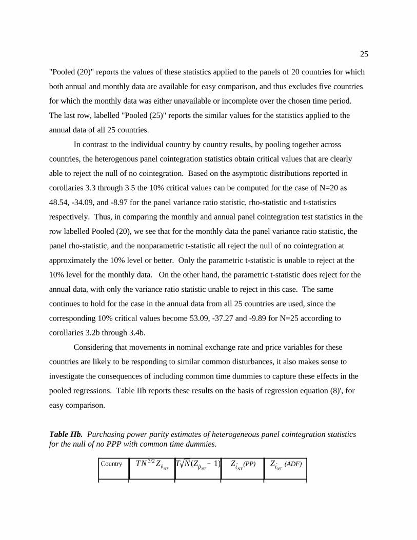
pooled regressions. Table IIb reports these results on the basis of regression equation (8)', for

easy comparison.

Table IIb. Purchasing power parity estimates of heterogeneous panel cointegration statisticsfor the null of no PPP with common time dummies.

Country (PP) (ADF)

sit ' "i % *t % $i pit % eit

26

Pooled (20) 36.20 * (62.07) * -37.03 * (-39.35) * -9.44 * (-9.53) * -11.47 (-7.84)

Pooled (25) 38.33 * -40.05 * -10.50 * -13.30

Notes: Estimated equation is (8)' : . Otherwise, all notes are same as for Table II.

Indeed, we see that for all but one of the 12 statistics reported, the results are strengthened by

the inclusion of the time dummies.

Finally, Table B.III of the appendix was constructed in order to indicate the closeness of

these asymptotic distributions to the empirical finite sample distributions for even relatively small

sized panels based on independent random walks, and this provides an alternative possibility for

comparing the estimated statistics. In this case, the approximate 10% critical values are

somewhat larger in absolute value, producing 54.97 (51.01), -33.05 (-34.99), and -9.77 (-9.13)

for the case of N=20, T=25 (T=250) for the heterogenous, demeaned panel variance ratio

statistic, panel rho-statistic, and panel t-statistics respectively according to Table B.III. On this

basis, the monthly data continues to reject for the panel variance ratio statistic and the panel rho

statistic, but the annual data produces statistics that fall slightly below the 10% empirical critical

values in this case in Table II, without time dummies. On the other hand, for N=25, T=25 the

empirical critical values based on the same Monte Carlo simulations produce 10% critical values

of 59.91, -36.03, and -10.77 respectively (not reported in the table). Thus, when the full sample

of 25 countries is used, even on the basis of small sample empirical distributions the annual data

continue to reject the null at the approximately the 10% level or better for the heterogenous

panel rho-statistic and parametric panel t-statistic. Evidently, this slight improvement likely

comes from the slightly larger size of the panel, which is just enough to boost the statistics to the

corresponding 10% critical value, rather than idiosyncratic features of the additional countries,

since individually they do not appear to disproportionately favor a rejection as compared to the

other twenty. Alternatively, the inclusion of common time dummies as in Table IIb appears to

preserve the rejections even for the most difficult case with only N=20 using annual data. Thus,

overall, on the basis of both the asymptotic critical values from section II and the empirical

Monte Carlo distributions of the appendix, the pooled data do appear to give fairly strong

support for the PPP hypothesis.

"i , $i

27

IV. Concluding Remarks

The intention of the purchasing power parity application has been to demonstrate the manner in

which the panel cointegration test statistics developed in this study can be successfully

implemented even for relatively small panel data sets. By specifying a cointegration hypothesis

that is considered to hold or not hold uniformly across members of a panel, the additional power

obtained from pooling the multivariate unit root information alone across the panel can be

sufficient to overturn results based on a member by member basis. More generally, one can

argue that, for the very same reasons that one would expect the long run structural parameters

to differ across countries, one might expect them to change over long periods of time for

any one country. In this case, one can also view pooling across members of a panel as a direct

alternative to increasing the time span of a single member over a period in which these

parameters may be changing. Either way, the broad applicability of such a procedure to

numerous other empirical issues should be apparent.

Needless to say, the empirical application to the PPP hypothesis also raises a number of

interesting issues, both empirical and methodological. For example, while empirical research has

not generally uncovered strong evidence for cross country cointegrating relationships among

exchange rates, the possibility certainly exists in many applications, including PPP. In this case,

it will be interesting to know how inclusion of possible intra-panel cointegrating relationships

under the null might affect the type of asymptotic distributions studied in this paper regarding the

existence of intra-member cointegrating relationships. Furthermore, the finite sample

distributions indicated by the Monte Carlo simulations in the appendix are performed for

independent random walks, and the extent to which they reliably indicate the properties of more

general finite sample regressions depends on the degree of temporal dependence present in the

data. It is well known that the for small time series dimensions, the size distortions from

estimating the asymptotic covariance matrix can be substantial in the case of high degrees of

serial correlation. Preliminary Monte Carlo evidence indicates, however, that under certain

conditions, the relative size distortions become much less severe as the number of cross sections

28

are increased. It will be interesting to consider such issues in future research, which is also

currently being undertaken.

29

REFERENCES

Abuaf and Jorion (1990) "Purchasing Power Parity in the Long Run," The Journal of Finance,45, 157-74.

Andrews, D. and C. Monahan (1992) "An Improved Heteroscadasticity and AutocorrelationConsistent Covariance Matrix," Econometrica, 60, 953-66.

Baillie and Selover (1987) "Cointegration and Model of Exchange Rate Deterimination,"International Journal of Forcasting, 3, 43-51.

Corbae, D. and S. Ouliaris (1988) "Cointegration and Tests of Purchasing Power Parity," Reviewof Economics and Statistics, 70, 508-11.

Campbell, J. and P. Perron (1991) "Pitfalls and Opportunities; What Macro-economists ShouldKnow About Unit Roots," NBER Macroeconomics Annual, 6.

Cheung, Y. and K Lai (1993) "Long-Run Purchasing Power Parity During the Recent Float,"Journal of International Economics, 34, 181-92.

Den Haan, W. and A. Levin (1995) "Inferences from parametric and non-parametric covariancematrix estimation procedures, International Finance Discussion Papers, No. 504.

Fisher E. and J. Park (1991) "Testing Purchasing Power Parity Under the Null Hypothesis ofCointegration," The Economic Journal, 101, 1476-84.

Holz-Eakon, D., W. Newey, and H. Rosen (1988) "Estimating Vector Autoregressions withPanel Data," Econometrica, 56.

Johansen, S. (1988) "Statistical Analysis of Cointegration Vectors," Journal of EconomicDynamics and Control, 12, 231-254.

Johansen, S. (1991) "Estimation and Hypothesis Testing of Cointegration Vectors in GaussianVector Autoregressive Models," Econometrica 59, 1551-80.

Lee, M. (1978) PURCHASING POWER PARITY, Dekker, New York.

Levin, A. and C. Lin (1994) "Unit Root Tests in Panel Data: Asymptotic and Finite-SampleProperties," University of California, San Diego Discussion Paper.

MacDonald, R. (1993) "Long-Run Purchasing Power Parity: Is it for Real?" Review ofEconomics and Statistics, 690-95.

30

Newey, W. and K. West (1987) "A Simple Positive Semi-Definite, Heteroscadasticity andAutocorrelation Consistent Covariance Matrix," Econometrica, 50, 703-8.

Park, J. and M Ogaki (1991) "Seemingly Unrelated Canonical Cointegrating Regressions," TheRochester Center for Economic Research, Working Paper No. 280.

Park, J. and M. Ogaki (1991) "Inference in Cointegrated Models Using VAR Prewhitening toEstimate Shortrun Dynamics," The Rochester Center for Economic Research, No. 281.

Park, J.Y. and P.C.B Phillips (1989) "Statistical Inference in Regressions with IntegratedProcesses: Part II," Econometric Theory, 5, 95-131.

Park, J.Y. and P.C.B Phillips (1988) "Statistical Inference in Regressions with IntegratedProcesses: Part I," Econometric Theory, 4, 468-497.

Patel, J. (1990) "Purchasing Power Parity as a Long Run Relation," Journal of AppliedEconometrics, 5, 367-79.

Pedroni P. (1993) "Endogenous Growth, Human Capital, and Cointegration for Multi-CountryPanels," Mimeo, Columbia University.

Perron, P. (1989) "Testing for a Random Walk: A Simulation Experiment of Power When theSampling Interval Is Varied," in B. Jaj, ed., Advances in Econometrics and modelling (KluwerAcademic Publishers, Dordrecht) 47 -68.

Perron, P. (1991) "Test Consistency with Varying Sampling Frequency," Econometric Theory, 7,341-68.

Phillips, P.C.B. (1986) "Understanding Spurious Regressions," Journal of Econometrics, 33,311-340.

Phillips, P.C.B. (1987) "Time Series Regression with a Unit Root," Econometrica, 55, 227-301.

Phillips and Durlauf, (1986) "Multiple Time Series Regression with Integrated Processes,"Review of Economic Studies, 53, 473-95.

Phillips, P. and Ouliaris (1990) "Asymptotic Properties of Residual Based Tests forCointegration, Econometrica, 58, 165-193.

Phillips, P. and P. Perron (1988) "Testing for a Unit Root in Time Series Regressions,Biometrika, 75, 335-346.

31

Pierce and Snell (1995) "Temporal Aggregation and the Power of Tests for a Unit Root,"Journal of Econometrics, 65, 333-45.

Quah, D. (1994) "Exploiting Cross-Section Variation for Unit Root Inference in Dynamic Data,"Economics Letters, 44, 9-19.

Shiller and Perron (1985) "Testing the Random Walk Hypothesis: Power Versus Frequency ofObservation, Economic Letters, 18, 381-86.

Taylor, M. (1988) "An Empirical Examination of Long-Run Purchasing Power Parity UsingCointegration Techniques," Applied Economics, 20, 1369-82.

N$NT '

1

Nj

N

i

T &2jT

t

xityit

1

N jN

i

T &2jT

t

x 2it

)6

1

Nj

N

i

S1/2i m

1

0Zi(r)Zi(r))drS1/2

i21

1

N jN

i

S1/2i m

1

0Zi(r) Zi(r))drS1/2

i22

~ Op(1)

T &1/2 t $NT' N $NT

T &1F2NT

1

N jN

i

(T &2jT

t

x 2it )

&1/2

~ Op(1)

1

Nj

N

i

T &2jT

t

xityit

1

N jN

i

T &2jT

t

x 2it

6

1

Nj

N

i

L11 iL22 im1

0ViWi % L21 iL22 im

1

0W 2

i

1

N jN

i

L 222 im

1

0W 2

i

Si ' S Op(1)

T &1F2NT '

1

N T 2 jN

ij

T

t

eit eit ~ I(1)

Zi(r)

A.1

(A1)

(A2)

(A3)

MATHEMATICAL APPENDIX

Proposition 2.1:

(a). Write

by virtue of (6a). If for all i, then the numerator converges to an randomvariable by a standard central limit theorem, and the denominator converges to a nonzeroconstant by the law of large numbers.

(b). Write

since converges to a nonzero constant for .

Lemma 2.1:

Expanding (A1) in terms of the elements of gives

where the index r has been dropped for notational convenience. Rearranging (A3) gives

N jN

i'1j

T

t'1

L &222 i x 2

it

&1

jN

i'1j

T

t'1

(L11 iL22 i)&1 xityit&

L21 i

L11 i

x 2it 6

1

Nj

N

i m1

0ViWi

1

N jN

i m1

0W 2

i

Vart m1

0

Wi(r)Vi(r)dr ' Et m1

0m1

0

Wi(r)Wi(s)Vi(r)Vi(s)dsdr

' 2 m1

0mq

0

EtWi(q)Wi(s)Vi(q)Vi(s)dsdq ' 2m1

0mq

0

s 2dsdq '1

6

Et m1

0

Wi(r)Vi(r)dr ' 0 ; Etm1

0

W 2i (r)dr ' m

1

0

rdr ' 1

2

T &1F2NT 6 1

N jN

i

L 211 imV 2

i % L11 iL21 imViWi % L 221 imW 2

i & $NT1

N mW 2i 6 1

2L 2

11 '1

2T11

Vi(r) ,Wi(r)

T21 ' 0 Si ' S L11 ' T11 &T2

21

T22

1/2

' T11

1

2L 2

22 '1

2T22

plimN,T64 $NT ' 0

eit' eit& ($& $)xit $ ' 0

A.2

(A4)

(A6)

(A5)

(A7)

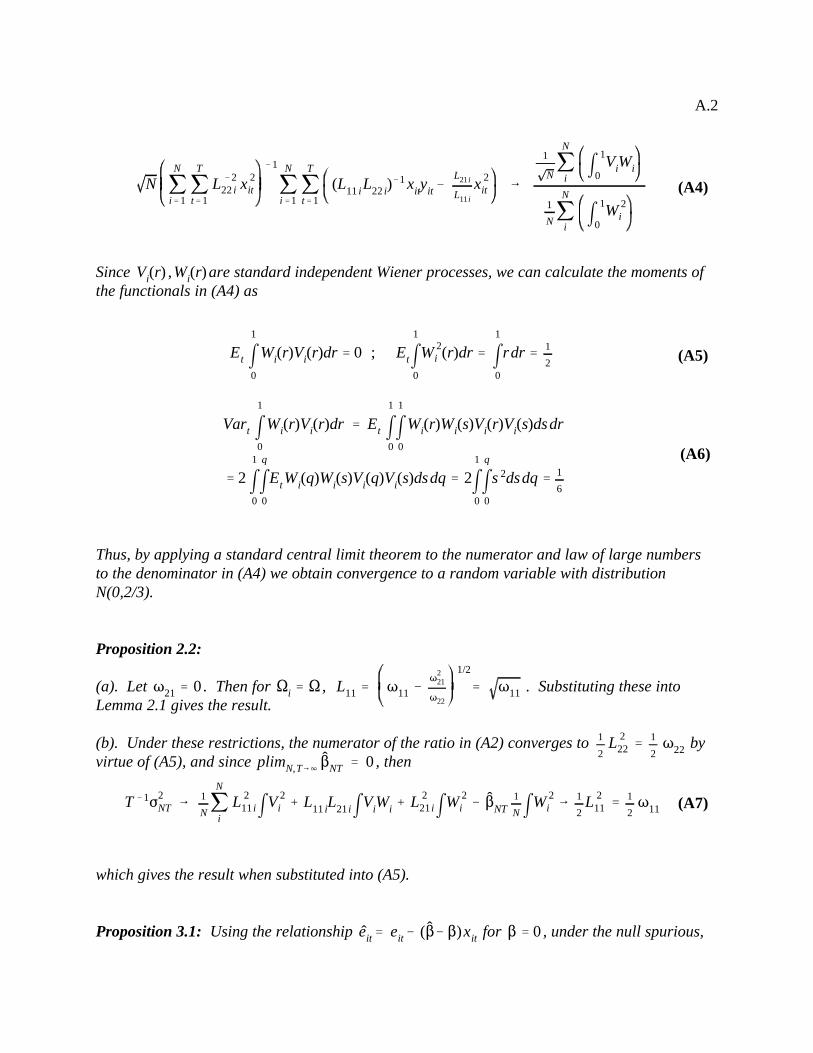
Since are standard independent Wiener processes, we can calculate the moments ofthe functionals in (A4) as

Thus, by applying a standard central limit theorem to the numerator and law of large numbersto the denominator in (A4) we obtain convergence to a random variable with distributionN(0,2/3).

Proposition 2.2:

(a). Let . Then for , . Substituting these intoLemma 2.1 gives the result.

(b). Under these restrictions, the numerator of the ratio in (A2) converges to byvirtue of (A5), and since , then

which gives the result when substituted into (A5).

Proposition 3.1: Using the relationship for , under the null spurious,

T (D&1) '

1

T jN

ij

T

t

eit&1)eit

1

T 2 jN

ij

T

t

e 2it&1

'

1

T NjN

ij

T

t

eit&1)eit &1

NN $ 1

T NjN

ij

T

t

xit&1)eit

1

T 2 Nj

N

ij

T

t

e 2it&1 &

1

NN$2 1

T 2 Nj

N

ij

T

t

x 2it&1

plimN,T641

T NjN

ij

T

t

eit&1)eit ' plimN,T641

T NjN

ij

T

t

eit&1)eit

plimN,T641

NT 2jN

ij

T

t

e 2it&1 ' plimN,T64

1

NT 2jN

ij

T

t

e 2it&1

T N(DNT&1) '

1

T Nj

N

ij

T

t

eit&1)eit

1

T 2Nj

N

ij

T

t

e 2it&1

6

1

T Nj

N

i

L 211m

1

0Vi dVi

1

T 2Nj

N

i

L 211m

1

0V 2

i

6 N(0,2)

$

$' $NT , N $ ~ Op (1) Op(1)Op(N

&1/2) Op(1)

$' $iT , N $ ~ Op (N 1/2) Op(1)

plimN,T $NT 6 0

A.3

(A8)

(A9)

(A10)

write

so that the terms that are subtracted from the numerator and denominator represent theinfluence on the distribution of estimating .

(a). For , so that the bracketed expressions are each and theentire subtracted terms each become , compared to the first terms which are . Thus, the contribution of the subtracted terms vanishes asymptotically, and

(b). For and the entire subtracted terms become so that theyare of the same order as the other terms. Thus, the influence of the subtracted term does notvanish asymptotically and condition (A9) does not hold.

Corollary 3.1:

(a). Since under the null from proposition 2.2(a), use (A9) to write

since the Brownian motion functional of the numerator has moments 0, 1/2 and the functionalof the denominator has mean 1/2.

1

T 2 NjN

ij

T

t

y 2it&1

&11

T Nj

N

ij

T

t

yit&1)yit '1

NjN

i

T &2jT

t

y 2it&1

&11

NjN

i

1

2(T &1/2YT)2 & T &1j

T

t

)yit

)yit ~ iid N(0,1) E [(T &1/2YiT)2]' 1, Var[(T &1/2YiT)2]' 2

E [T &1jT

t

)yit]' T &1 Var[T &1jT

t

)yit]' 2T &2

E [T &2jT

t

y 2it&1]' T &2j

T

t

E [y 2it&1]' T &2j

T

t

(t&1) ' 1

2T (T&1) N64

N(0,T(T&1) /T 2) 1

2T(T&1) /T 2

F 6 F ' 1 as N64

A.4

(b). Again, using the results of proposition 3.1, write the rho-statistic in terms of y as

where for , we have ,

and

. Thus, as , the numerator

converges to and the denominator converges to , so that taken

together these give the stated result.

(c). For the t-statistic, with iid disturbances, , and the remainder of the denominator converges to the square root of the term to which the denominator of the rho-statistic converges, giving the stated result.

/

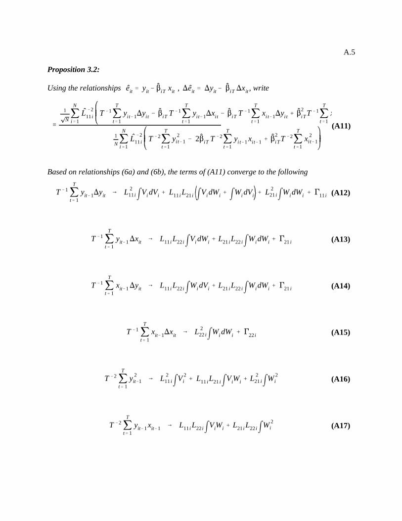
1

NjN

i'1

L&211 i T &1j

T

t'1

yi t&1)yi t & $iT T &1jT

t'1

yi t&1)xi t & $iT T &1jT

t'1

xi t&1)yi t % $2iTT &1j

T

t'1

x

1

N jN

i'1L

&211 i T &2j

T

t'1y 2

i t&1 & 2$iT T &2jT

t'1yi t&1 xi t&1 % $2

iTT &2jT

t'1x 2

i t&1

T &1 jT

t' 1yit&1)yit 6 L 2

11 imVi dVi % L11 i L21 i mVidWi % mWi dVi % L 221 imWidWi % '11 i

T &1 jT

t' 1yit&1)xit 6 L11 i L22 imVi dWi % L21 iL22 imWidWi % '21 i

T &1 jT

t' 1xit&1)yit 6 L11 i L22 imWi dVi % L21 iL22 imWidWi % '21 i

T &1 jT

t' 1

xit&1)xit 6 L 222 imWi dWi % '22 i

T &2 jT

t' 1y 2

it&1 6 L 211 imV 2

i % L11 iL21 imViWi % L 221 imW 2

i

T &2 jT

t' 1yit&1 xit&1 6 L11 i L22 imViWi % L21 i L22 imW 2

i

eit ' yit& $iT xit )eit ' )yit& $iT )xit

A.5

(A11)

(A12)

(A13)

(A14)

(A15)

(A16)

(A17)

Proposition 3.2:

Using the relationships , , write

Based on relationships (6a) and (6b), the terms of (A11) converge to the following

T &2 jT

t' 1x 2

it&1 6 L 222 imW 2

i

$iT 6L11 iL22 imViWi % L21 iL22 imW 2

i

L 222 imW 2

i

1) 6

1

NjN

i'1L

&211 i L 2

11 i mVidVi &mViWi

mW 2i

mVi dWi % mWi dVi % mViWi

mW 2i

2

mWi dWi

1

N jN

i'1L

&211 i L 2

11 i mV 2i & mViWi

2

mW 2i

6

1

N

1

N

/ 1

N jN

i'1

L&211 i F

2iT 6 1

N jN

i'1

L&211 i L 2

11 i % L 221 i & 2$iT L21 i L22 i % $2

iT L 222 i 6 1

N jN

i'1

L&211 i L 2

11 i % L 211 i

mViW

mW2i

ZtDNT

6

1

NjN

i'1 mQidQi

1

N jN

i'1 mQ 2i 1% 1

N jN

i'1

$2i

QiSi L11 i 6 L11 i T64

µ it ' )eit & (D & 1) ei t&1 6 )eit D61T64 T &1j

t

)Zit)Z )

it ' T &1jt

>it>)

it 6 L )

i Li ' Si F2NT

TN 3/2 ZvNT

A.6

(A18)

(A19)

(A22)

Furthermore, setting N=1 in (A3) gives

Thus, substituting expressions (A12) through (A19) into (A11) gives (A20)

where the last convergency is based on the definition of from Lemma 3.1 and consistentestimation of , based for example on (5), so that as .

For the t-statistics, considider that since as. Thus, given that , the term can be

evaluated as (A21)

where the last convergency is obtained by substituting in the square of expression (A19). Hence

The statistic is given simply by setting the numerator of (A20) to unity. Thus, the

TN 3/2 ZvNT& 1&1

y N 6 N N &1jN

i'1

Ky i

&1

& (1y )&1

NT& 1) & 1x1

&1y N 6 N N &1j

N

i'1Kx i & 1x N &1j

N

i'1Ky i

&1

% 1x N N &1jN

i'1Ky i

&1

&

ZtNT& 1x1

&1/2y (1%1z)

&1/2 N 6 N N &1jN

i'1

Kx i& 1x N &1jN

i'1

Ky i

&1/2

N &1jN

i'1

Kz i

&1/

N N &1jN

i'1

Ky i

&1/2

& (1y )&1/2 N &1jN

i'1

Kz i

&1/2

% 1x1&1/2y N N &1j

N

i'1

Kz i

&1/2

& (1%1

ZN ' N g N &1jN

i'1

Xi & g(µ) 6 N(0,")E")

K / (mQ 2,mQdQ, $2))

N64

ZN XiE

N64 " "i 'dg

dg i

(µ i)µ i' 1i , E' R(i) , "' N(i)

A.7

(A23)

(A24)

(A25)

(A26)

distributions of each of these statistics is free of nuisance parameters and will be governed onlyby the first two moments of the vector Brownian motion functional .

To obtain the precise relationship in terms of these moments, rewrite the statistics as

where indices y,x,z have been used in place of 1,2,3 respectively. As , the summations incurved brackets converge to the means of the respective random variables by virtue of a law oflarge numbers. This leaves the expressions involving each of the square bracketed terms as acontinuously differentiable transformation of a sum of i.i.d. random variables. In general, for acontinuously differential transformation of an i.i.d. vector sequence with vector mean uand covariance ,

as , where the ith element of the vector is given by the partial derivative (cf. Dhrymes, 1974). Thus, setting for each of the statistics providesthe desired results.

Corollaries 3.2-3.4:

Expanding the terms for the variances in proposition 3.2 gives

T N (ZDNT& 1) & 1x1

&1y N 6 N (0 , 1&2

y Rx& 1&2x 1& 4

y Ry& 21x1&3y Rxy )

T N ZvNT& 1&1

y N 6 N( 0, 1& 4y Ry )

T N ZtNT& 1x (1y (1%1z))

&1/2 N 6 N( 0,. )

%1z)&1Rx %

1

412

x1&3y (1%1z)

&1Ry %1

412

x1&1y (1%1z)

&3Rz & 1x1&2y (1%1z)

&1Rxy &1x1&1y (1%1z)

&2Rxz %1

212

x1&2y (

N64

A.8

(A28)

(A27)

(A29)

where

.

Substituting the empirical moments for large T , N=1 into these expressions gives the reportedapproximations for the asymptotic distributions as .