Julia Vallejo, Francisco R. Fortea-Pérez, Emilio Pardo ... · S3 Physical Techniques. Elemental...

S1

Electronic Supporting Information (ESI) for the manuscript:

Guest-Dependent Single-Ion Magnet Behaviour in a Cobalt(II) Metal-Organic Framework

Julia Vallejo, Francisco R. Fortea-Pérez, Emilio Pardo,* Samia Benmansour, Isabel Castro, J.

Krzystek, Donatella Armentano and Joan Cano*

Electronic Supplementary Material (ESI) for Chemical Science.This journal is © The Royal Society of Chemistry 2015

S2

Experimental Section

Materials. All chemicals were of reagent grade quality, and they were purchased from

commercial sources and used as received.

1,4-bis(4'-Pyridylethynyl)benzene(bpeb). The bpeb ligand was synthesized by using a slightly

modified previously reported procedure.1 The only difference can be found in the final step where,

instead of recrystallizing the residue from toluene, it was purified by thoroughly washing with cold

water and ether. The product was isolated as a yellow solid. Yield 99%. IR (KBr): 2220 (νC C). 1H

NMR (CDCl3): 7.41 (4H, d), 7.58 (4H, s), 8.64 (4H, d). 13C NMR (CDCI3): 88.6, 93.2 (C C),

123.0, 125.5, 131.2, 132.0, 149.9.

Preparation of [Co(bpeb)2(NCS)2]·7DCB (DCB@1). Well-formed orange cubic prisms of

DCB@1, suitable for X-ray diffraction, were grown after a few days of slow layer diffusion in an

essay tube at room temperature. The top layer was a methanol solution of the CoII(NCS)2 (0.0088 g,

0.05 mmol), while the bottom one was a dichlorobenzene/methanol solution (4:1 v/v) of the bpeb

ligand (0.028 g, 0.1 mmol). The crystals were collected by filtration and air-dried (0.040 g, 42%

yield); elemental analysis calculated (%) for C84H52Cl14CoN6S2 (1756.9): C 57.17, H 2.97, N 4.76,

S 3.63; found: C 56.96, H 3.11, N 4.56, S 3.69. IR (KBr) 2080((νNCS), 1497, 1590 (νC=C) and 2218

cm–1 (νC C).

Preparations of [Co(bpeb)2(NCS)2].4TAN.4MeOH (TAN@1), [Co(bpeb)2(NCS)2].6TOL

(TOL@1) and [Co(bpeb)2(NCS)2].8PYR (PYR@1). Well-formed orange cubic prism of

TAN@1, TOL@1 and PYR@1, which were suitable for X-ray diffraction, were obtained by

immersing crystals of DCB@1 for a week in thianthrene, toluene and pyrrole solutions,

respectively. The crystals were collected by filtration and air-dried. TAN@1: elemental analysis

calculated (%) for C94H72CoN6 O4S10 (1727.2): C 65.29, H 4.20, N 4.86, S18.54; found: C 64.98, H

4.35, N 4.90, S 18.60, IR (KBr) 2080(νNCS), 1462, 1495, 1590 (νC=C) and 2219 cm–1 (νC C).

TOL@1: elemental analysis calculated (%) for C84H72CoN6S2 (1287.5): C 78.30, H 5.63, N 6.52, S

4.98; found: C 78.36, H 5.85, N 6.47, S 4.97. IR (KBr) 2081(νNCS), 3087, 3062(νCH3), 1497,

1590(νC=C) and 2218 cm–1 (νC C). PYR@1: elemental analysis calculated (%) for C74H64CoN14S2

(1271.4): C 69.85, H 5.07, N 15.41, S 5.04; found: C 69.97, H 4.96, N 15.46, S 5.01. IR (KBr)

2080(νNCS), 3400(νNH) 1494, 1589 (νC=C) and 2218 cm–1 (νC C).

1 Champness, N. R.; Khlobystov, A. N.; Majuga, A. G.; Schröder, M.; Zyk, N. V. Tetrahedron Lett. 1999, 40 (29),

5413.

S3

Physical Techniques. Elemental (C, H, S, N) and Inductively coupled plasma–atomic emission

spectroscopy (ICP-AES) analyses were performed at the Microanalytical Service of the Universitat

de València.

Thermogravimetric Analysis. The thermogravimetric analysis (TGA) was performed on

crystalline samples of DCB@1, TAN@1, TOL@1 and PYR@1 under a dry N2 atmosphere with a

Mettler Toledo TGA/STDA 851e thermobalance operating at a heating rate of 10 ºC min–1.

X-ray Powder Diffraction. Polycrystalline samples of DCB@1, TAN@1, TOL@1 and

PYR@1 were introduced into 0.5 mm borosilicate capillaries prior to being mounted and aligned

on a Empyrean PANalytical powder diffractometer, using Cu Kα radiation (λ = 1.54056 Å). For

each sample, three repeated measurements were collected at 100 K (2θ = 2–40°) and merged in a

single diffractogram.

HFEPR Measurements. HFEPR spectra of DCB@1, TAN@1, TOL@1 and PYR@1 were

recorded at 4.5 K on polycrystalline samples (20-25 mg) suspended in the corresponding solvent

(see experimental section) to prevent any possible desolvation, using a homodyne spectrometer

associated with a 15/17-T superconducting magnet. The presence of solvent strongly restricted the

frequency to values lower than ~ 200 GHz. Detection was provided with an InSb hot electron

bolometer (QMC Ltd., Cardiff, UK). The magnetic field was modulated at 50 kHz for detection

purposes. A Stanford Research Systems SR830 lock-in amplifier converted the modulated signal to

dc voltage. The single-frequency spectra were simulated with the SPIN software.

Crystal Structure Data Collection and Refinement. Crystal data for DCB@1:

C84H52Cl14CoN6S2, triclinic, space group P(-1), a = 13.593(5) Å, b = 17.194(5) Å, c = 18.450(5)

Å, α = 99.319(5)°, = 100.076(5)°, = 107.842(5)° V = 3933(2) Å3, T = 100(2) K, Z = 2,

ρcalc = 1.490 g.cm-3, μ = 0.797 mm-1, of the 59588 reflections collected (Rint = 0.0526), 8262 are

unique and 5878 observed with I > 2σ(I). Refinement of 386 parameters gave R = 0.1485 and

Rw = 0.3876 for reflections with I > 2σ(I) and R = 0.1824 and Rw = 0.4104 for all reflections, with

S = 1.483. TAN@1: C94H72CoN6O4S10 monoclinic, space group C2/m, a = 13.8432(9) Å,

b = 20.8218(9) Å, c = 14.0803(6) Å, = 96.987(3)°, V = 4028.4(3) Å3, T = 100(2) K, Z = 2,




S = 1.073. TOL@1: C84H72CoN6S2, monoclinic, space group C2/c, a = 31.601(4) Å, b = 21.039(4)

S4

Å, c = 27.275(5) Å, = 121.629(11)°, V = 15440(5) Å3, T = 100(2) K, Z = 8, ρcalc = 1.109 g.cm-3,

μ = 0.321 mm-1, of the 55448 reflections collected (Rint = 0.0892), 13092 are unique and 5828

observed with I > 2σ(I). Refinement of 467 parameters gave R = 0.0872 and Rw = 0.2189 for

reflections with I > 2σ(I) and R = 0.1581 and Rw = 0.2372 for all reflections, with S = 1.054.

PYR@1: C74H64CoN14S2, triclinic, space group P(-1), a = 11.653(4) Å, b = 13.567(6) Å, c =

13.662(6) Å, α = 94.50(2)°, = 94.78(2)°, = 111.12(2)° V = 1994.0(14) Å3, T = 100(2) K, Z = 1,,




S = 1.886.

Single crystals of DCB@1, TAN@1, TOL@1 and PYR@1 were selected and mounted on a

MITIGEN holder in Paratone oil and very quickly placed on a liquid nitrogen stream cooled at 100

K to avoid the possible degradation upon desolvation. Diffraction data were collected on a Bruker-

Nonius X8APEXII CCD area detector diffractometer using graphite-monochromated Mo-Kα

radiation ( = 0.71073 Å). As reported, crystals of DCB@1, TAN@1, TOL@1 and PYR@1,

suitable for X-ray diffraction, were obtained by immersing crystals of DCB@1 for a week in

thianthrene, toluene and pyrrole solutions, respectively, after a crystal-to-crystal transformation

accounting for a poor quality and a poor diffraction power of the samples. In fact, a lower θmax of

diffraction were obtained, especially for PYR@1, even if all possible steps were undertaken to

ensure that the experiment was able to extract the best diffracting power from the sample. However,

since the solution and refinement parameters are reasonable, compared with analogue 2D MOFs

structures previously reported, we are confident that the crystal structure found is consistent. The

data were processed through the SAINT2 reduction and SADABS3 multi-scan absorption software.

The structure was solved with the ShelXS structure solution program, using the Direct Methods

solution method. The model was refined with version 2013/4 of ShelXL against F2 on all data by

full-matrix least squares.4 All non-hydrogen atoms were refined anisotropically. The hydrogen

atoms of the organic ligands were set on geometrical positions and refined with a riding model.

Keeping in mind that we are dealing with a SC to SC solid-state incorporation of the solvent guests

into the 2D networks, it is not surprising that the thianthrene, toluene and pyrrole molecules found

from F map were disordered within the voids of the structure. In particular, no good model for

2 SAINT, version 6.45, Bruker Analytical X-ray Systems, Madison, WI, 2003. 3 Sheldrick G.M. SADABS Program for Absorption Correction, version 2.10, Analytical X-ray Systems, Madison, WI,

2003 4 (a) G. M. Sheldrick, Acta Cryst. 2008, A64, 112-122. (b) SHELXTL-2013/4, Bruker Analytical X-ray Instruments,

Madison, WI, 2013.

S5

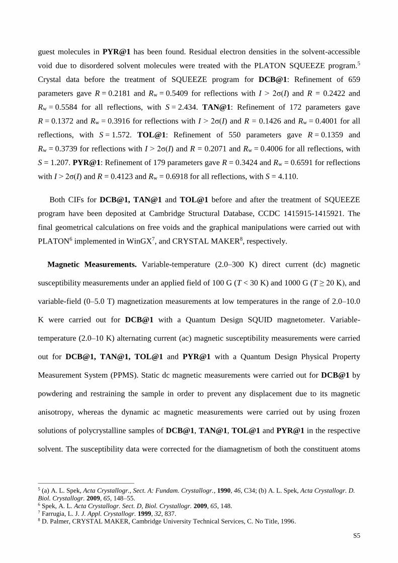
guest molecules in PYR@1 has been found. Residual electron densities in the solvent-accessible

void due to disordered solvent molecules were treated with the PLATON SQUEEZE program.5

Crystal data before the treatment of SQUEEZE program for DCB@1: Refinement of 659

parameters gave R = 0.2181 and Rw = 0.5409 for reflections with I > 2σ(I) and R = 0.2422 and

Rw = 0.5584 for all reflections, with S = 2.434. TAN@1: Refinement of 172 parameters gave

R = 0.1372 and Rw = 0.3916 for reflections with I > 2σ(I) and R = 0.1426 and Rw = 0.4001 for all

reflections, with S = 1.572. TOL@1: Refinement of 550 parameters gave R = 0.1359 and


S = 1.207. PYR@1: Refinement of 179 parameters gave R = 0.3424 and Rw = 0.6591 for reflections

with I > 2σ(I) and R = 0.4123 and Rw = 0.6918 for all reflections, with S = 4.110.

Both CIFs for DCB@1, TAN@1 and TOL@1 before and after the treatment of SQUEEZE

program have been deposited at Cambridge Structural Database, CCDC 1415915-1415921. The

final geometrical calculations on free voids and the graphical manipulations were carried out with

PLATON6 implemented in WinGX7, and CRYSTAL MAKER8, respectively.

Magnetic Measurements. Variable-temperature (2.0–300 K) direct current (dc) magnetic

susceptibility measurements under an applied field of 100 G (T < 30 K) and 1000 G (T ≥ 20 K), and

variable-field (0–5.0 T) magnetization measurements at low temperatures in the range of 2.0–10.0

K were carried out for DCB@1 with a Quantum Design SQUID magnetometer. Variable-

temperature (2.0–10 K) alternating current (ac) magnetic susceptibility measurements were carried

out for DCB@1, TAN@1, TOL@1 and PYR@1 with a Quantum Design Physical Property

Measurement System (PPMS). Static dc magnetic measurements were carried out for DCB@1 by

powdering and restraining the sample in order to prevent any displacement due to its magnetic

anisotropy, whereas the dynamic ac magnetic measurements were carried out by using frozen

solutions of polycrystalline samples of DCB@1, TAN@1, TOL@1 and PYR@1 in the respective

solvent. The susceptibility data were corrected for the diamagnetism of both the constituent atoms

5 (a) A. L. Spek, Acta Crystallogr., Sect. A: Fundam. Crystallogr., 1990, 46, C34; (b) A. L. Spek, Acta Crystallogr. D.

Biol. Crystallogr. 2009, 65, 148–55. 6 Spek, A. L. Acta Crystallogr. Sect. D, Biol. Crystallogr. 2009, 65, 148. 7 Farrugia, L. J. J. Appl. Crystallogr. 1999, 32, 837. 8 D. Palmer, CRYSTAL MAKER, Cambridge University Technical Services, C. No Title, 1996.

S6

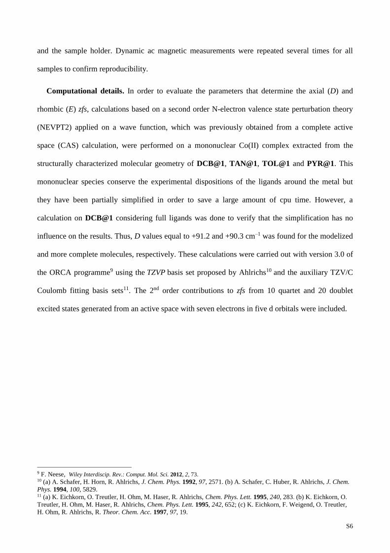
and the sample holder. Dynamic ac magnetic measurements were repeated several times for all

samples to confirm reproducibility.

Computational details. In order to evaluate the parameters that determine the axial (D) and

rhombic (E) zfs, calculations based on a second order N-electron valence state perturbation theory

(NEVPT2) applied on a wave function, which was previously obtained from a complete active

space (CAS) calculation, were performed on a mononuclear Co(II) complex extracted from the

structurally characterized molecular geometry of DCB@1, TAN@1, TOL@1 and PYR@1. This

mononuclear species conserve the experimental dispositions of the ligands around the metal but

they have been partially simplified in order to save a large amount of cpu time. However, a

calculation on DCB@1 considering full ligands was done to verify that the simplification has no

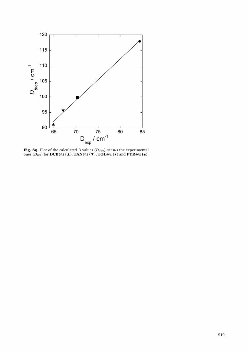
influence on the results. Thus, D values equal to +91.2 and +90.3 cm–1 was found for the modelized

and more complete molecules, respectively. These calculations were carried out with version 3.0 of

the ORCA programme9 using the TZVP basis set proposed by Ahlrichs10 and the auxiliary TZV/C

Coulomb fitting basis sets11. The 2nd order contributions to zfs from 10 quartet and 20 doublet

excited states generated from an active space with seven electrons in five d orbitals were included.

9 F. Neese, Wiley Interdiscip. Rev.: Comput. Mol. Sci. 2012, 2, 73. 10 (a) A. Schafer, H. Horn, R. Ahlrichs, J. Chem. Phys. 1992, 97, 2571. (b) A. Schafer, C. Huber, R. Ahlrichs, J. Chem.

Phys. 1994, 100, 5829. 11 (a) K. Eichkorn, O. Treutler, H. Ohm, M. Haser, R. Ahlrichs, Chem. Phys. Lett. 1995, 240, 283. (b) K. Eichkorn, O.

Treutler, H. Ohm, M. Haser, R. Ahlrichs, Chem. Phys. Lett. 1995, 242, 652; (c) K. Eichkorn, F. Weigend, O. Treutler,

H. Ohm, R. Ahlrichs, R. Theor. Chem. Acc. 1997, 97, 19.

S7

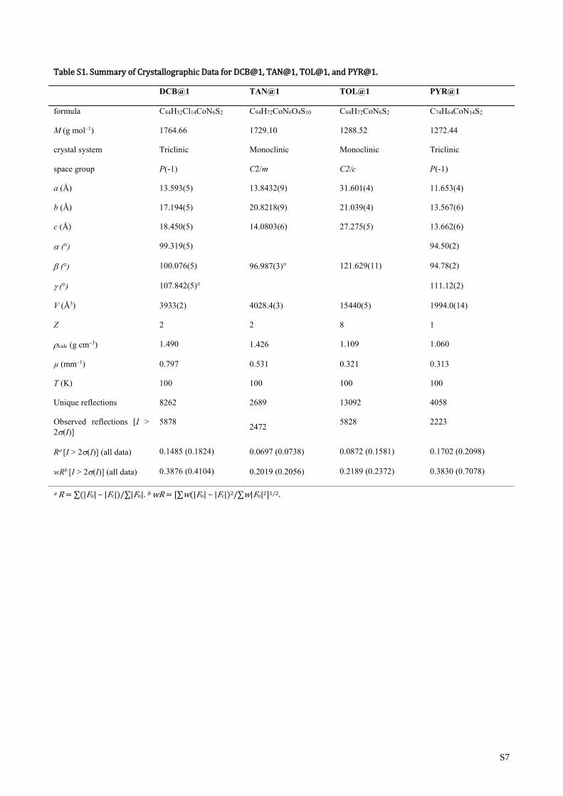
Table S1. Summary of Crystallographic Data for DCB@1, TAN@1, TOL@1, and PYR@1.

DCB@1 TAN@1 TOL@1 PYR@1

formula C84H52Cl14CoN6S2 C94H72CoN6O4S10 C84H72CoN6S2 C74H64CoN14S2

M (g mol–1) 1764.66 1729.10 1288.52 1272.44

crystal system Triclinic Monoclinic Monoclinic Triclinic

space group P(-1) C2/m C2/c P(-1)

a (Å) 13.593(5) 13.8432(9) 31.601(4) 11.653(4)

b (Å) 17.194(5) 20.8218(9) 21.039(4) 13.567(6)

c (Å) 18.450(5) 14.0803(6) 27.275(5) 13.662(6)

(°) 99.319(5) 94.50(2)

(°) 100.076(5) 96.987(3)° 121.629(11) 94.78(2)

(°) 107.842(5)° 111.12(2)

V (Å3) 3933(2) 4028.4(3) 15440(5) 1994.0(14)

Z 2 2 8 1

calc (g cm–3) 1.490 1.426 1.109 1.060

µ (mm–1) 0.797 0.531 0.321 0.313

T (K) 100 100 100 100

Unique reflections 8262 2689 13092 4058

Observed reflections [I >

2(I)]

5878 2472

5828 2223

Ra [I > 2(I)] (all data) 0.1485 (0.1824) 0.0697 (0.0738) 0.0872 (0.1581) 0.1702 (0.2098)

wRb [I > 2(I)] (all data) 0.3876 (0.4104) 0.2019 (0.2056) 0.2189 (0.2372) 0.3830 (0.7078)

a R = ∑(|Fo| – |Fc|)/∑|Fo|. b wR = [∑w(|Fo| – |Fc|)2/∑w|Fo|2]1/2.

S8

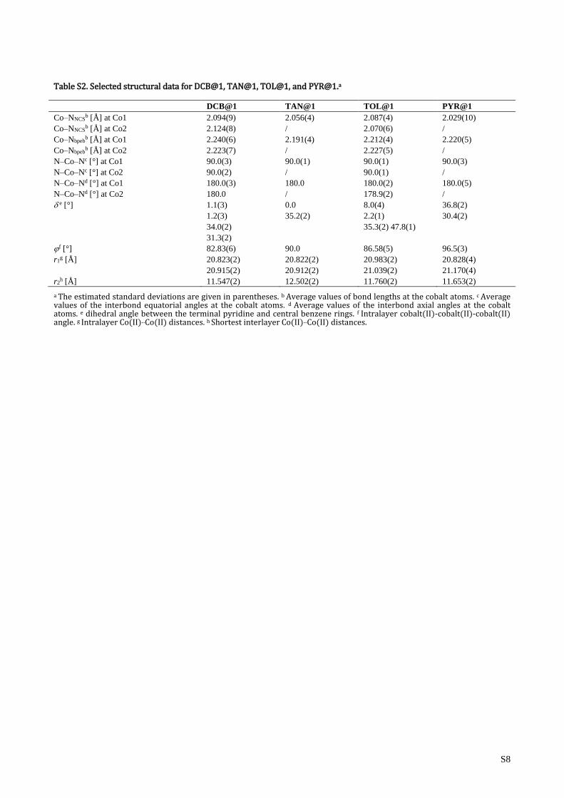
Table S2. Selected structural data for DCB@1, TAN@1, TOL@1, and [email protected]

DCB@1 TAN@1 TOL@1 PYR@1

Co–NNCSb [Å] at Co1 2.094(9) 2.056(4) 2.087(4) 2.029(10)

Co–NNCSb [Å] at Co2 2.124(8) / 2.070(6) /

Co–Nbpebb [Å] at Co1 2.240(6) 2.191(4) 2.212(4) 2.220(5)

Co–Nbpebb [Å] at Co2 2.223(7) / 2.227(5) /

N–Co–Nc [°] at Co1 90.0(3) 90.0(1) 90.0(1) 90.0(3)

N–Co–Nc [°] at Co2 90.0(2) / 90.0(1) /

N–Co–Nd [°] at Co1 180.0(3) 180.0 180.0(2) 180.0(5)

N–Co–Nd [°] at Co2 180.0 / 178.9(2) /

e [°] 1.1(3)

1.2(3)

34.0(2)

31.3(2)

0.0

35.2(2)

8.0(4)

2.2(1)

35.3(2) 47.8(1)

36.8(2)

30.4(2)

f [°] 82.83(6) 90.0 86.58(5) 96.5(3)

r1g [Å] 20.823(2)

20.915(2)

20.822(2)

20.912(2)

20.983(2)

21.039(2)

20.828(4)

21.170(4)

r2h [Å] 11.547(2) 12.502(2) 11.760(2) 11.653(2)

a The estimated standard deviations are given in parentheses. b Average values of bond lengths at the cobalt atoms. c Average values of the interbond equatorial angles at the cobalt atoms. d Average values of the interbond axial angles at the cobalt atoms. e dihedral angle between the terminal pyridine and central benzene rings. f Intralayer cobalt(II)-cobalt(II)-cobalt(II) angle. g Intralayer Co(II)...Co(II) distances. h Shortest interlayer Co(II)...Co(II) distances.

S9

Table S3. Selected ac magnetic data for DCB@1, TAN@1, TOL@1, and PYR@1 at different dc applied fields.

Compound Ha (G) 0(1)b 107 (s) 0(2)b 105 (s)

Eab (cm−1) c S

c (cm3 mol−1) Tc (cm3 mol−1)

DCB@1 250 0.23 0.55

29.9 7.6

0.033 (4K) 0.012 (5K) 0.023 (6K)

0.14 (4K) 0.11 (5K) 0.09 (6K)

0.32 (4K) 0.26 (5K) 0.21 (6K)

DCB@1 500 0.27 0.48

29.2 8.6

0.023 (4K) 0.012 (5K) 0.009 (6K)

0.05 (4K) 0.04 (5K) 0.04 (6K)

0.32 (4K) 0.26 (5K) 0.21 (6K)

DCB@1 1000 0.17 0.41

31.3 8.8

0.024 (4K) 0.015 (5K) 0.012 (6K)

0.01 (4K) 0.01 (5K) 0.01 (6K)

0.32 (4K) 0.26 (5K) 0.21 (6K)

TAN@1 1000 2.27 0.78

17.1 6.2

0.058 (4K) 0.027 (5K) 0.017 (6K)

0.02 (4K) 0.01 (5K) 0.01 (6K)

0.30 (4K) 0.24 (5K) 0.20 (6K)

TOL@1 1000 8.22 3.00

11.5 2.5

0.071 (4K) 0.075 (5K)

0.062 (5.5K)

0.03 (4K) 0.02 (5K)

0.01 (5.5K)

0.28 (4K) 0.23 (5K)

0.20 (5.5K)

PYR@1 1000 1.30 1.02

21.0 4.9

0.073 (4K) 0.124 (5K) 0.105 (6K)

0.03 (4K) 0.02 (5K) 0.01 (6K)

0.24 (4K) 0.19 (5K) 0.16 (6K)

a Applied dc magnetic field. b The values of the pre-exponential factor (τ0) and activation energy (Ea) are calculated through the Arrhenius law [ = ((1/01) exp(Ea1/kBT) + (1/02) exp(Ea2/kBT))–1].c The values of the parameter, adiabatic (S) and isothermal (T) susceptibilities are calculated from the experimental data at different temperatures through the generalized Debye law (see text).

S10

Table S4. Exponent of a power-law probability distributions (n) of relaxation times () with the temperature (–1 = CTn) of DCB@1, TAN@1 , TOL@1 and PYR@1 in a 1.0 kG applied static field.

Compound H (G) n C

DCB@1 1000 4.07 39.9

TAN@1 1000 3.39 171

TOL@1 1000 2.66 819

PYR@1 1000 2.87 412

S11

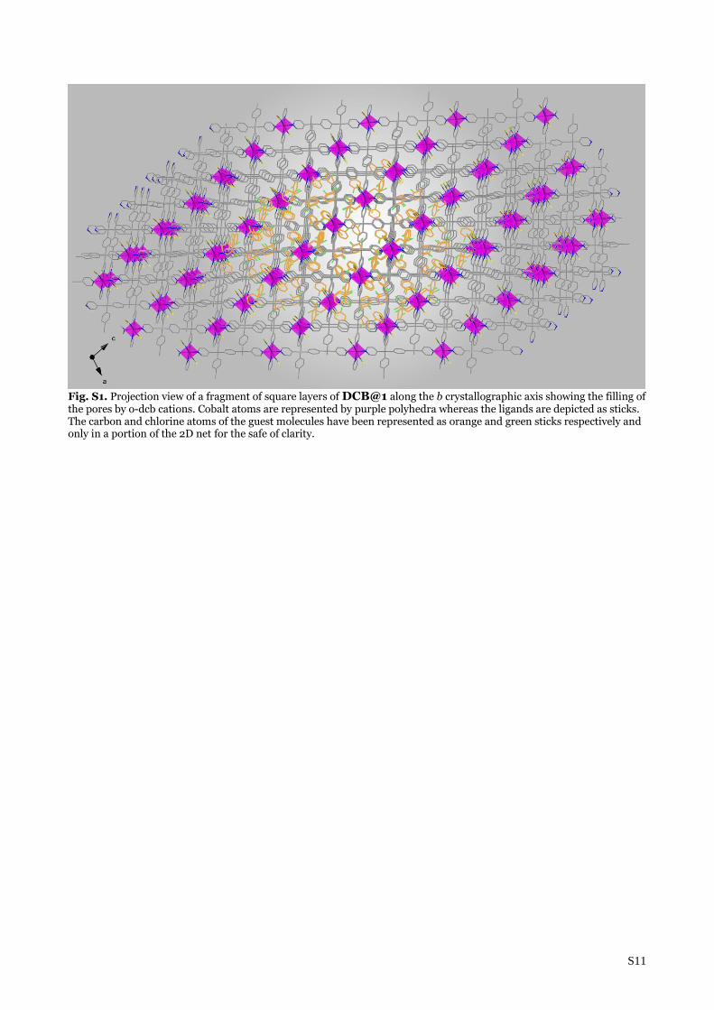
Fig. S1. Projection view of a fragment of square layers of DCB@1 along the b crystallographic axis showing the filling of the pores by o-dcb cations. Cobalt atoms are represented by purple polyhedra whereas the ligands are depicted as sticks. The carbon and chlorine atoms of the guest molecules have been represented as orange and green sticks respectively and only in a portion of the 2D net for the safe of clarity.

S12

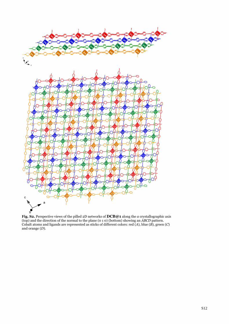
Fig. S2. Perspective views of the pilled 2D networks of DCB@1 along the a crystallographic axis (top) and the direction of the normal to the plane (0 1 0) (bottom) showing an ABCD pattern. Cobalt atoms and ligands are represented as sticks of different colors: red (A), blue (B), green (C) and orange (D).

S13

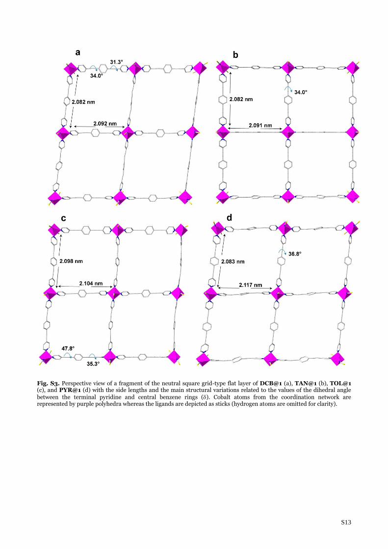
Fig. S3. Perspective view of a fragment of the neutral square grid-type flat layer of DCB@1 (a), TAN@1 (b), TOL@1 (c), and PYR@1 (d) with the side lengths and the main structural variations related to the values of the dihedral angle between the terminal pyridine and central benzene rings (). Cobalt atoms from the coordination network are represented by purple polyhedra whereas the ligands are depicted as sticks (hydrogen atoms are omitted for clarity).

S14

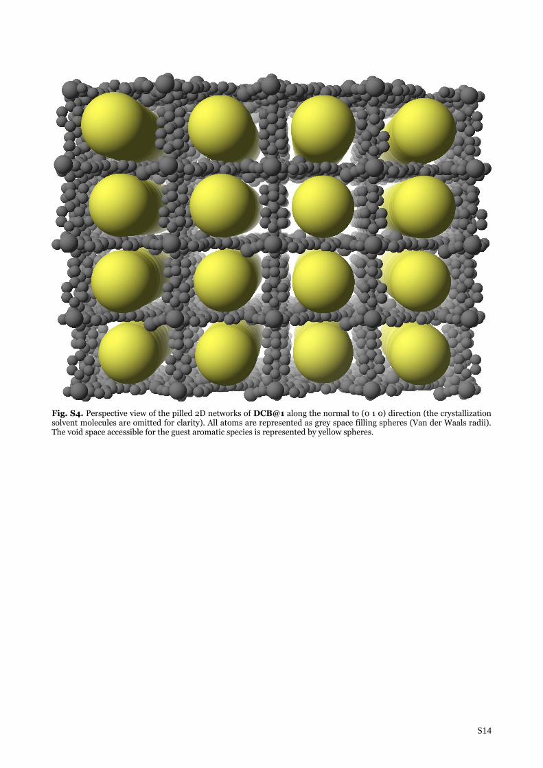
Fig. S4. Perspective view of the pilled 2D networks of DCB@1 along the normal to (0 1 0) direction (the crystallization solvent molecules are omitted for clarity). All atoms are represented as grey space filling spheres (Van der Waals radii). The void space accessible for the guest aromatic species is represented by yellow spheres.

S15

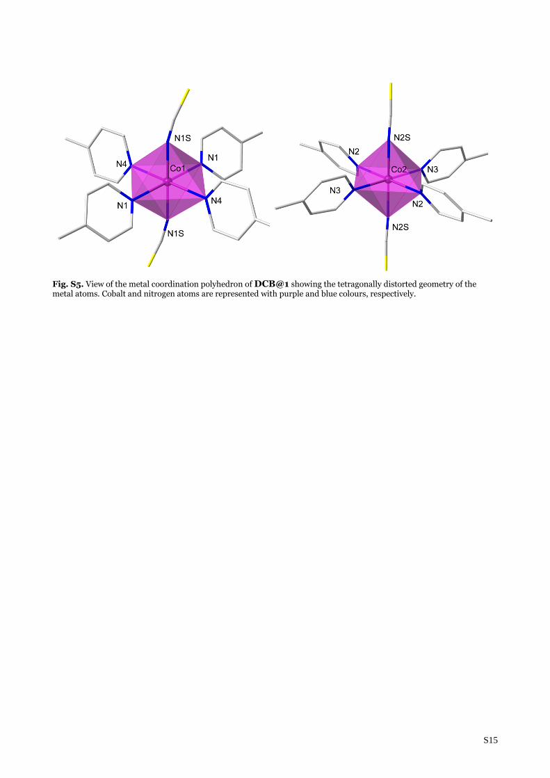
Fig. S5. View of the metal coordination polyhedron of DCB@1 showing the tetragonally distorted geometry of the metal atoms. Cobalt and nitrogen atoms are represented with purple and blue colours, respectively.

S16

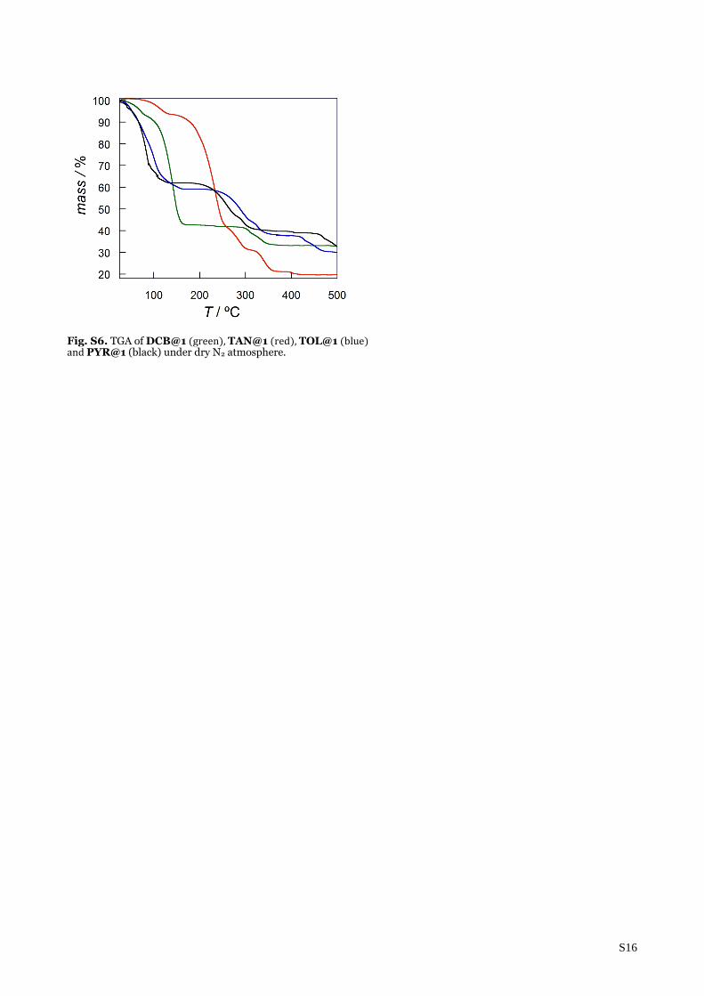
Fig. S6. TGA of DCB@1 (green), TAN@1 (red), TOL@1 (blue) and PYR@1 (black) under dry N2 atmosphere.

S17

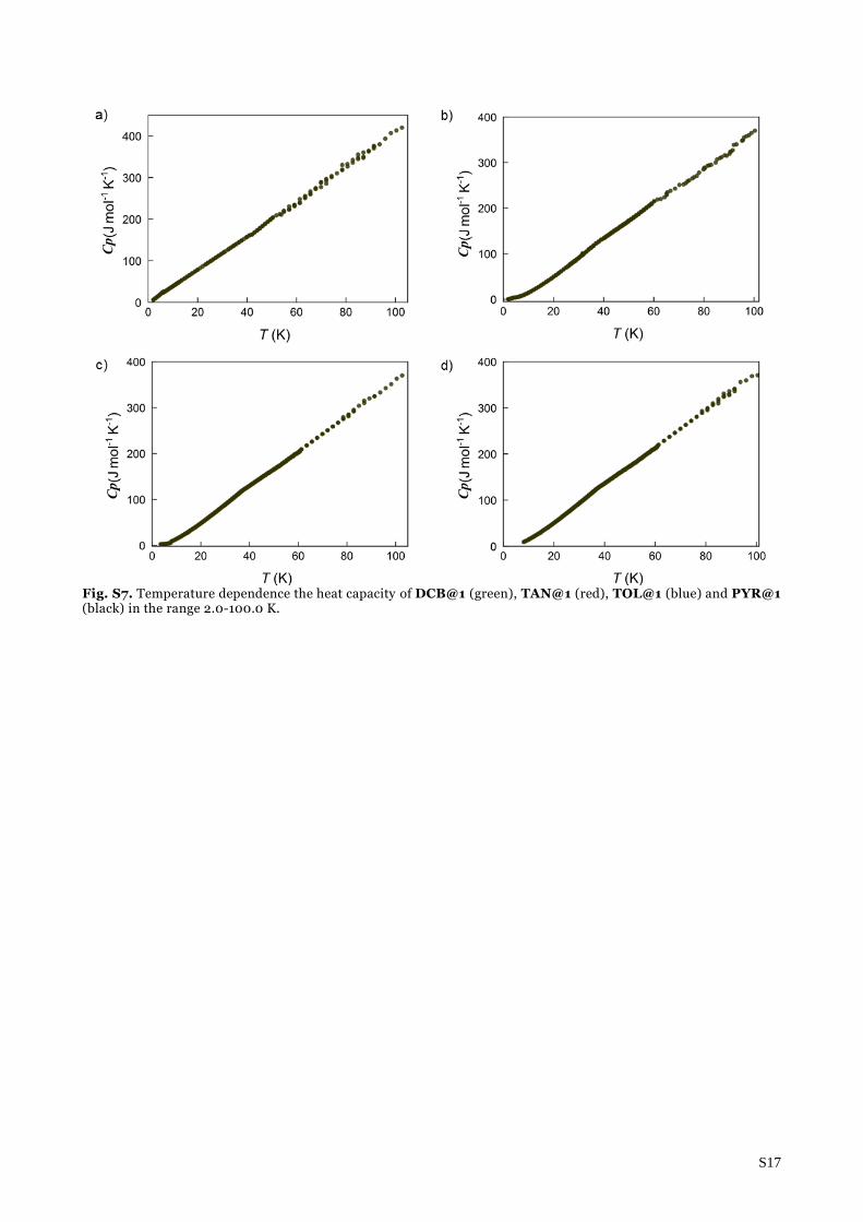
Fig. S7. Temperature dependence the heat capacity of DCB@1 (green), TAN@1 (red), TOL@1 (blue) and PYR@1 (black) in the range 2.0-100.0 K.

S18

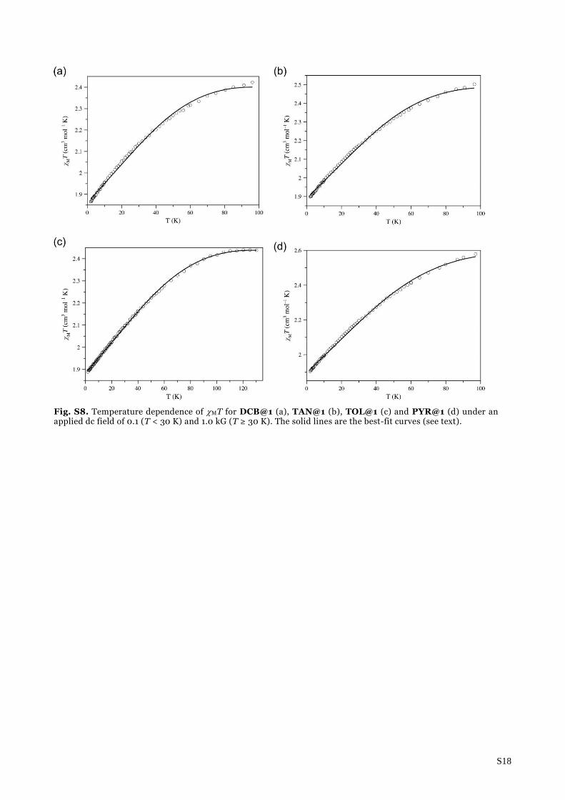
Fig. S8. Temperature dependence of MT for DCB@1 (a), TAN@1 (b), TOL@1 (c) and PYR@1 (d) under an applied dc field of 0.1 (T < 30 K) and 1.0 kG (T ≥ 30 K). The solid lines are the best-fit curves (see text).

S19

Fig. S9. Plot of the calculated D values (Dtheo) versus the experimental ones (Dexp) for DCB@1 (▲), TAN@1 (▼), TOL@1 (●) and PYR@1 (■).

S20

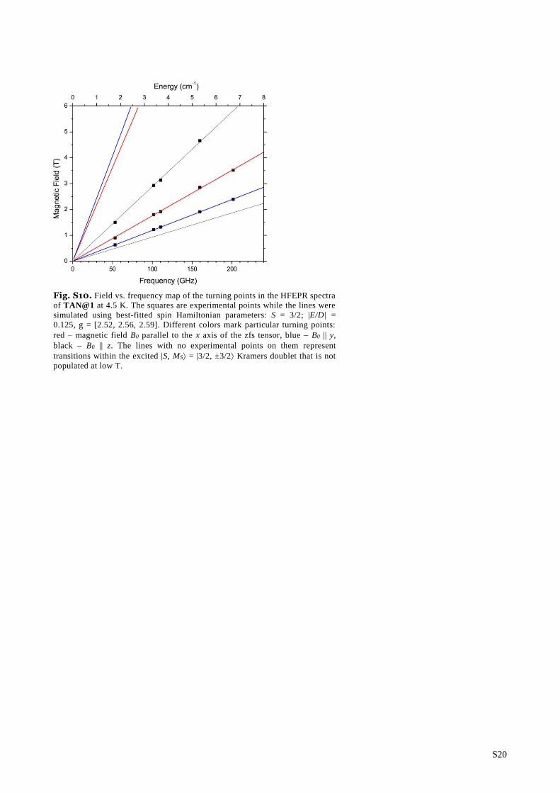
Fig. S10. Field vs. frequency map of the turning points in the HFEPR spectra

of TAN@1 at 4.5 K. The squares are experimental points while the lines were

simulated using best-fitted spin Hamiltonian parameters: S = 3/2; |E/D| =

0.125, g = [2.52, 2.56, 2.59]. Different colors mark particular turning points:

red – magnetic field B0 parallel to the x axis of the zfs tensor, blue B0 || y,

black B0 || z. The lines with no experimental points on them represent

transitions within the excited |S, MS = |3/2, ±3/2 Kramers doublet that is not

populated at low T.

S21

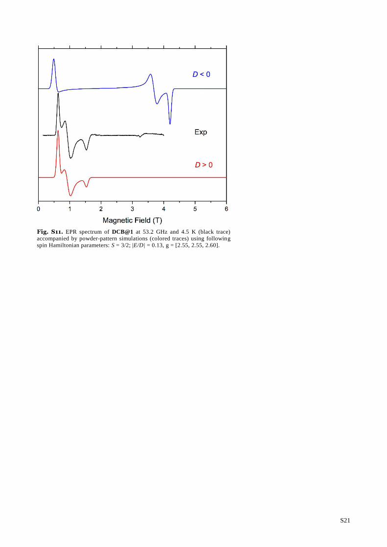
Fig. S11. EPR spectrum of DCB@1 at 53.2 GHz and 4.5 K (black trace)

accompanied by powder-pattern simulations (colored traces) using following

spin Hamiltonian parameters: S = 3/2; |E/D| = 0.13, g = [2.55, 2.55, 2.60].

S22

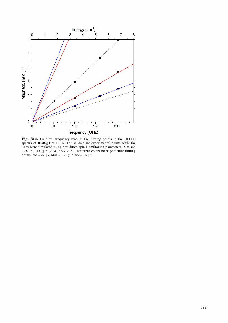
Fig. S12. Field vs. frequency map of the turning points in the HFEPR

spectra of DCB@1 at 4.5 K. The squares are experimental points while the

lines were simulated using best-fitted spin Hamiltonian parameters: S = 3/2;

|E/D| = 0.13, g = [2.54, 2.56, 2.59]. Different colors mark particular turning

points: red – B0 || x, blue B0 || y, black B0 || z.

S23

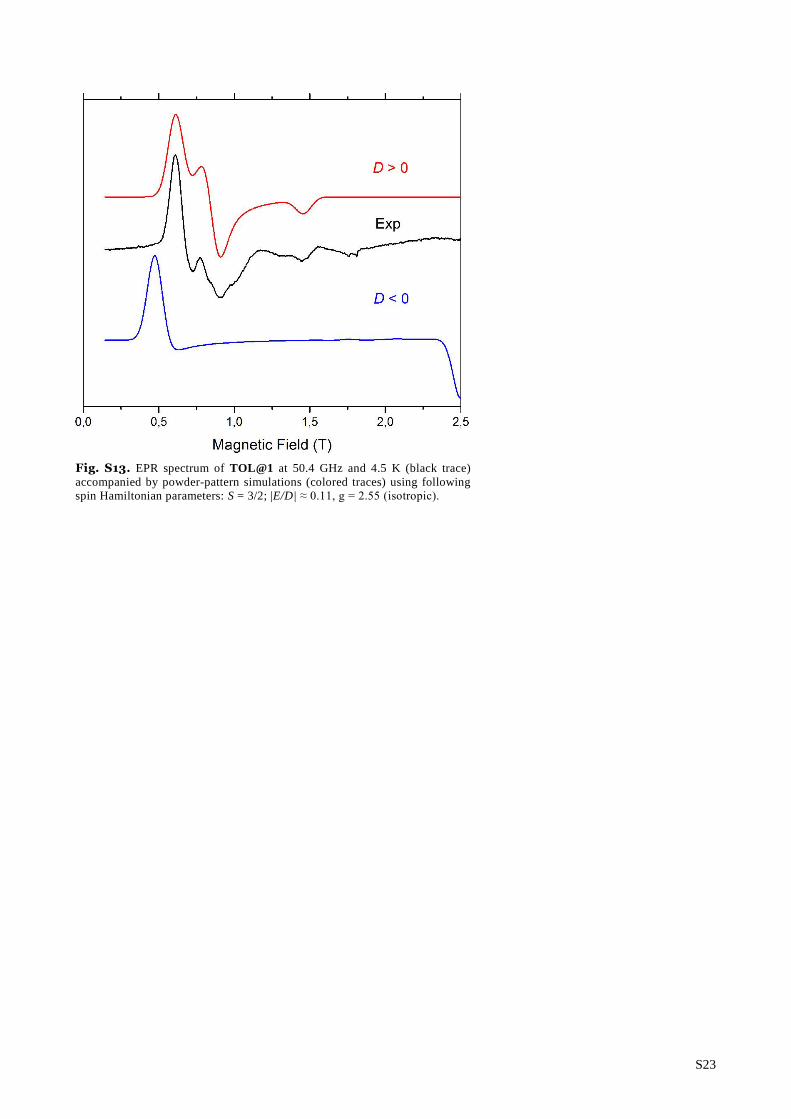
Fig. S13. EPR spectrum of TOL@1 at 50.4 GHz and 4.5 K (black trace)


spin Hamiltonian parameters: S = 3/2; |E/D| ≈ 0.11, g = 2.55 (isotropic).

S24

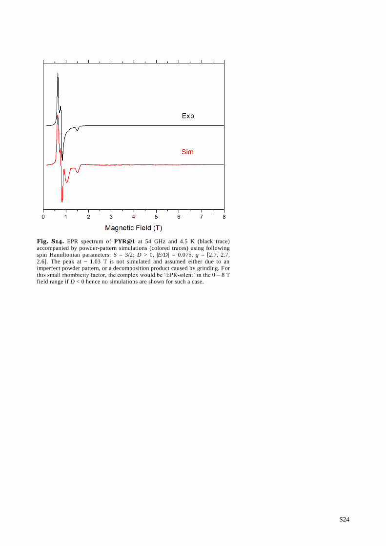
Fig. S14. EPR spectrum of PYR@1 at 54 GHz and 4.5 K (black trace)


spin Hamiltonian parameters: S = 3/2; D > 0, |E/D| = 0.075, g = [2.7, 2.7,

2.6]. The peak at ~ 1.03 T is not simulated and assumed either due to an

imperfect powder pattern, or a decomposition product caused by grinding. For

this small rhombicity factor, the complex would be ‘EPR-silent’ in the 0 – 8 T

field range if D < 0 hence no simulations are shown for such a case.

S25

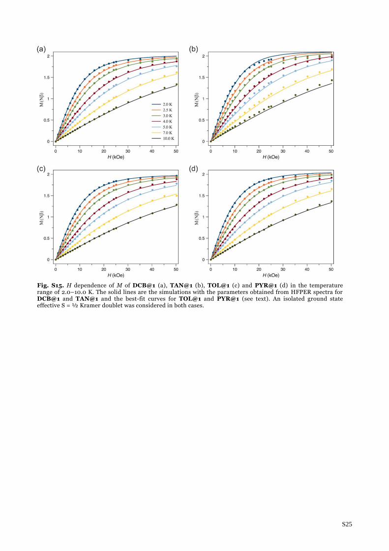
Fig. S15. H dependence of M of DCB@1 (a), TAN@1 (b), TOL@1 (c) and PYR@1 (d) in the temperature range of 2.0–10.0 K. The solid lines are the simulations with the parameters obtained from HFPER spectra for DCB@1 and TAN@1 and the best-fit curves for TOL@1 and PYR@1 (see text). An isolated ground state effective S = ½ Kramer doublet was considered in both cases.

S26

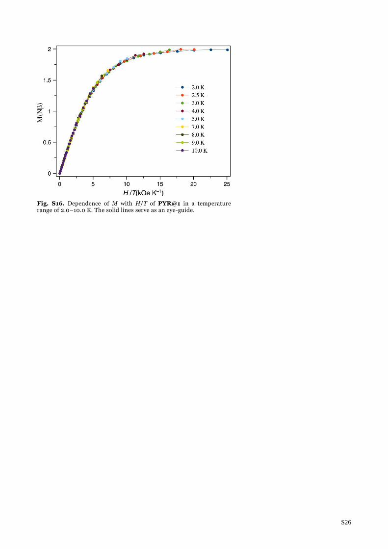
Fig. S16. Dependence of M with H/T of PYR@1 in a temperature range of 2.0–10.0 K. The solid lines serve as an eye-guide.

S27

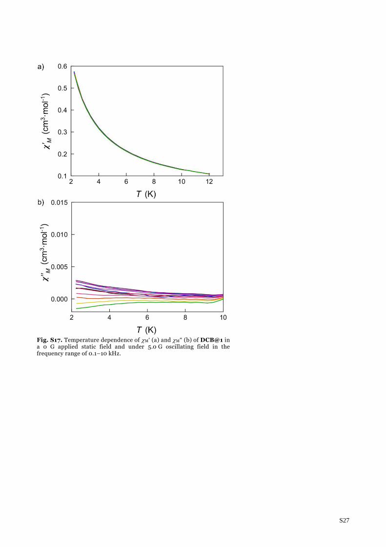
Fig. S17. Temperature dependence of M‘ (a) and M“ (b) of DCB@1 in a 0 G applied static field and under 5.0 G oscillating field in the frequency range of 0.1–10 kHz.

S28

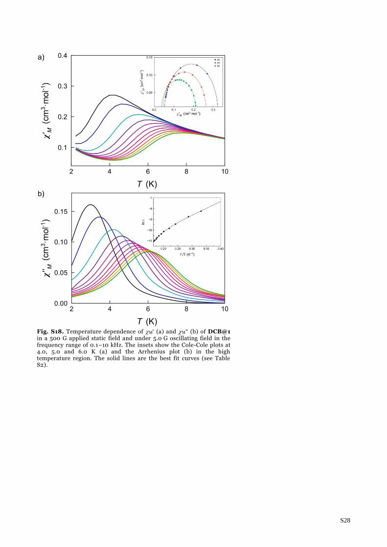
Fig. S18. Temperature dependence of M‘ (a) and M“ (b) of DCB@1 in a 500 G applied static field and under 5.0 G oscillating field in the frequency range of 0.1–10 kHz. The insets show the Cole-Cole plots at 4.0, 5.0 and 6.0 K (a) and the Arrhenius plot (b) in the high temperature region. The solid lines are the best fit curves (see Table S2).

S29

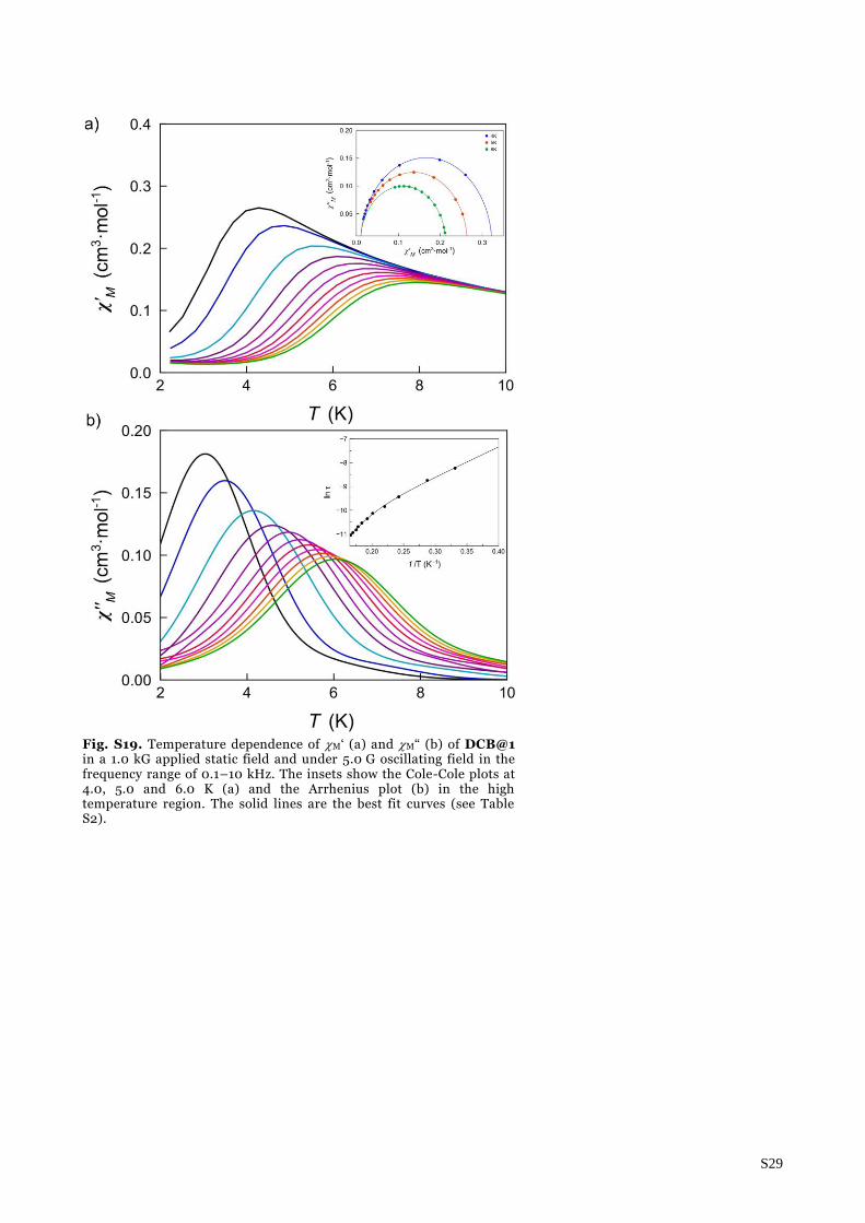
Fig. S19. Temperature dependence of M‘ (a) and M“ (b) of DCB@1 in a 1.0 kG applied static field and under 5.0 G oscillating field in the frequency range of 0.1–10 kHz. The insets show the Cole-Cole plots at 4.0, 5.0 and 6.0 K (a) and the Arrhenius plot (b) in the high temperature region. The solid lines are the best fit curves (see Table S2).

S30

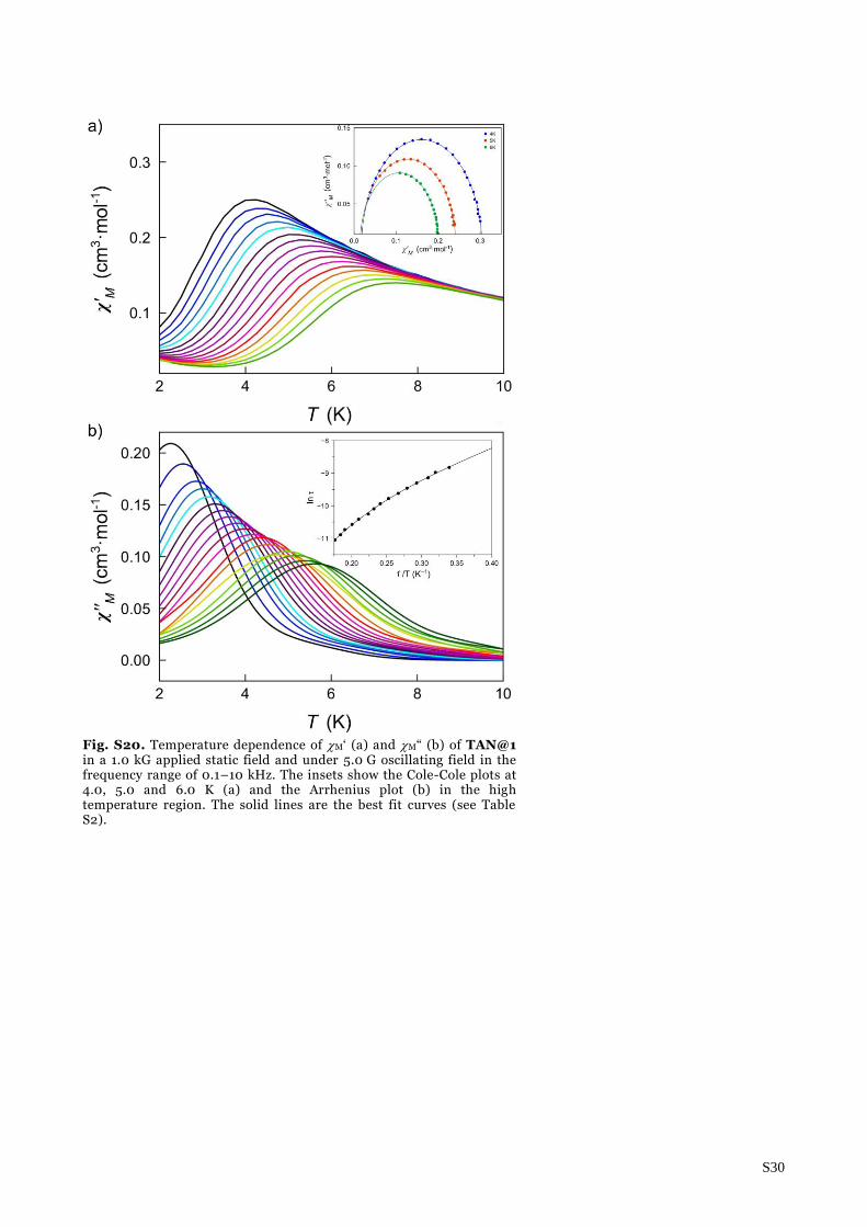
Fig. S20. Temperature dependence of M‘ (a) and M“ (b) of TAN@1 in a 1.0 kG applied static field and under 5.0 G oscillating field in the frequency range of 0.1–10 kHz. The insets show the Cole-Cole plots at 4.0, 5.0 and 6.0 K (a) and the Arrhenius plot (b) in the high temperature region. The solid lines are the best fit curves (see Table S2).

S31

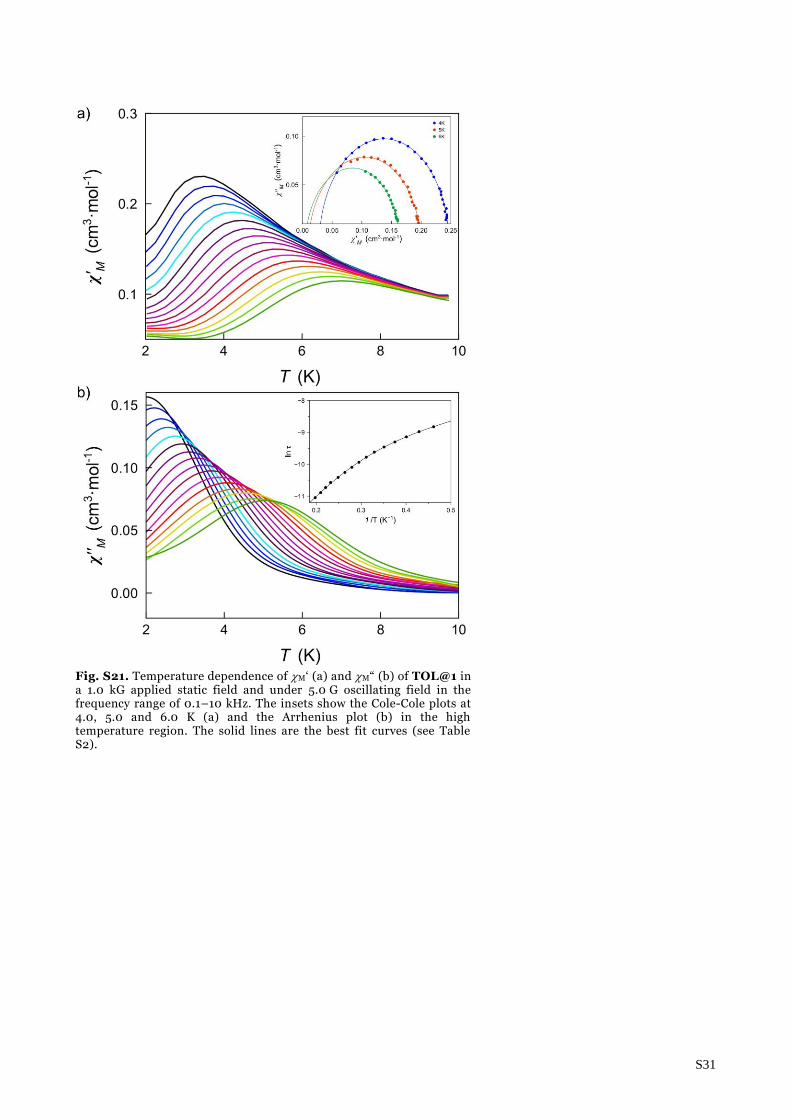
Fig. S21. Temperature dependence of M‘ (a) and M“ (b) of TOL@1 in a 1.0 kG applied static field and under 5.0 G oscillating field in the frequency range of 0.1–10 kHz. The insets show the Cole-Cole plots at 4.0, 5.0 and 6.0 K (a) and the Arrhenius plot (b) in the high temperature region. The solid lines are the best fit curves (see Table S2).

S32

Fig. S22. Temperature dependence of M‘ (a) and M“ (b) of PYR@1 in a 1.0 kG applied static field and under 5.0 G oscillating field in the frequency range of 0.1–10 kHz. The insets show the Cole-Cole plots at 4.0, 5.0 and 5.5 K (a) and the Arrhenius plot (b) in the high temperature region. The solid lines are the best fit curves (see Table S2).

S33

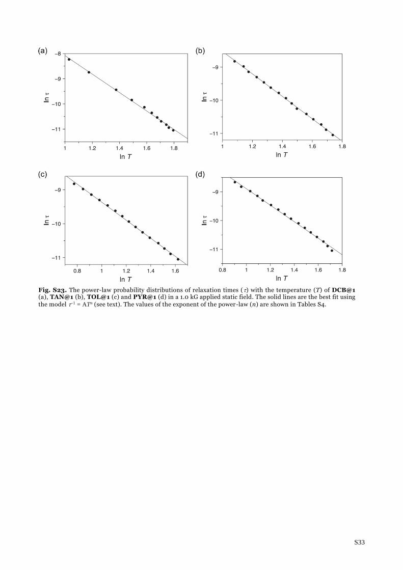
Fig. S23. The power-law probability distributions of relaxation times () with the temperature (T) of DCB@1 (a), TAN@1 (b), TOL@1 (c) and PYR@1 (d) in a 1.0 kG applied static field. The solid lines are the best fit using the model –1 = ATn (see text). The values of the exponent of the power-law (n) are shown in Tables S4.

Julia Vallejo, Francisco R. Fortea-Pérez, Emilio Pardo ... · S3 Physical Techniques. Elemental...

Documents

Transcript of Julia Vallejo, Francisco R. Fortea-Pérez, Emilio Pardo ... · S3 Physical Techniques. Elemental...