Jules Bloomenthal - Princeton University Computer … · Implicit Surfaces Jules Bloomenthal...

Implicit Surfaces

Jules Bloomenthal

Unchained Geometry, Seattle

Introduction

Implicit surfaces are two-dimensional, geometric shapes that exist in three dimensional space.

They are defined according to a particular mathematical form. This article examines their

definition, representation, and geometric properties. Related fields are discussed and practical

methods are reviewed.

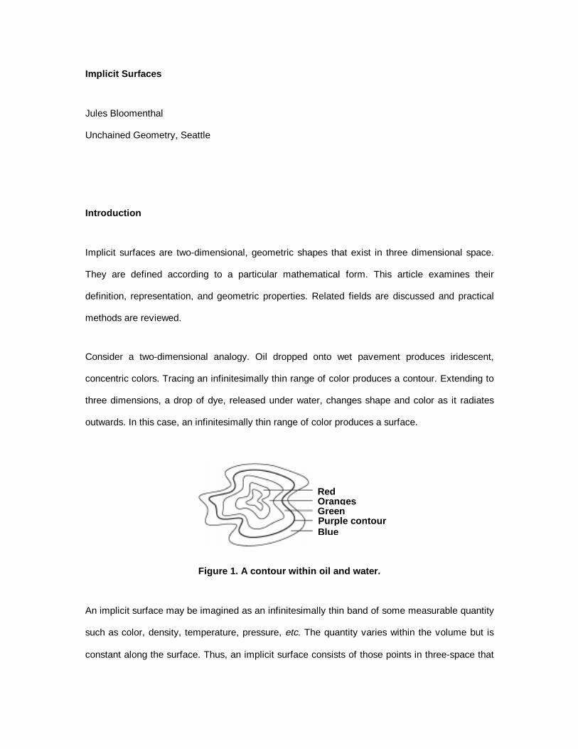
Consider a two-dimensional analogy. Oil dropped onto wet pavement produces iridescent,

concentric colors. Tracing an infinitesimally thin range of color produces a contour. Extending to

three dimensions, a drop of dye, released under water, changes shape and color as it radiates

outwards. In this case, an infinitesimally thin range of color produces a surface.

Figure 1. A contour within oil and water.

An implicit surface may be imagined as an infinitesimally thin band of some measurable quantity

such as color, density, temperature, pressure, etc. The quantity varies within the volume but is

constant along the surface. Thus, an implicit surface consists of those points in three-space that

RedOrangesGreenPurple contourBlue

satisfy some particular requirement. Mathematically, the requirement is represented by a

function f, whose argument is a three-dimensional point p.

By definition, if f(p) = 0 then p is on the surface. f inherently characterizes a volume: those

points for which f < 0 are on one side (nominally the ‘inside’) of the surface, those points for

which f > 0 are on the other side of the same surface. f does not explicitly describe the surface,

but implies its existence. For many functions, f is proportional to the distance between p and the

surface. This and other attributes encourage particular forms of geometric design.

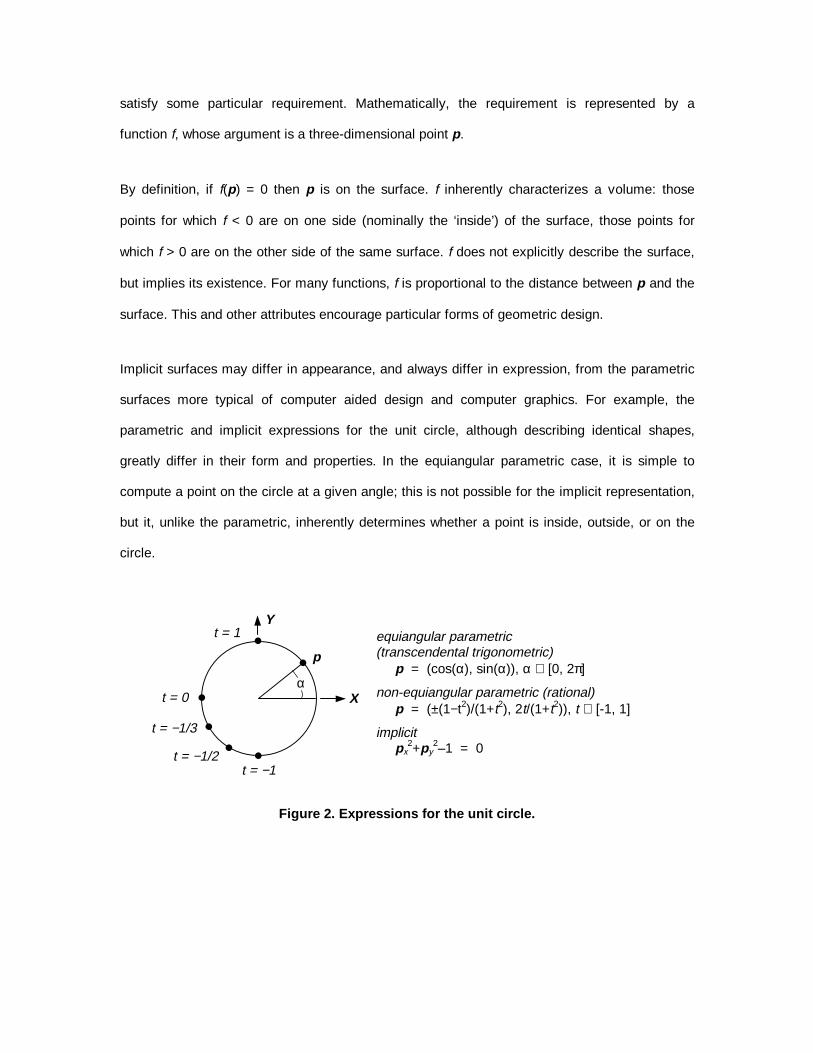
Implicit surfaces may differ in appearance, and always differ in expression, from the parametric

surfaces more typical of computer aided design and computer graphics. For example, the

parametric and implicit expressions for the unit circle, although describing identical shapes,

greatly differ in their form and properties. In the equiangular parametric case, it is simple to

compute a point on the circle at a given angle; this is not possible for the implicit representation,

but it, unlike the parametric, inherently determines whether a point is inside, outside, or on the

circle.

Figure 2. Expressions for the unit circle.

equiangular parametric(transcendental trigonometric)

p = (cos(α), sin(α)), α ∈ [0, 2π]

non-equiangular parametric (rational)p = (±(1−t2)/(1+t2), 2t/(1+t2)), t ∈ [-1, 1]

implicitpx

2+py2–1 = 0

α

p

t = 1

t = 0

t = −1/3

t = −1/2t = −1

X

Y

Mathematical Foundations

Analytic geometry is the branch of mathematics devoted to the relationship between geometry

and the mathematical expression of the coordinates of points in space. When applied in three

dimensions, it is called solid analytic geometry. If geometric relationships between points in

three-space are compared to corresponding mathematical (i.e., algebraic) relationships between

the coordinates (x, y, and z) of the points, it is possible by algebraic proof to establish a

geometric property. For example, the distance between the centers of two spheres can be

compared algebraically with the sum of their radii, thereby predicting whether the spheres

intersect geometrically.

Analytic geometry has been applied to a wide variety of mathematical functions to establish their

properties (especially tangency) and to enable their graphical display. The relationship between

the coordinates of points on a geometric object is fundamental to geometric design.

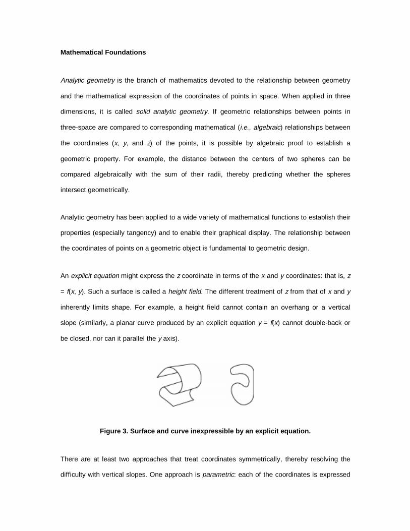
An explicit equation might express the z coordinate in terms of the x and y coordinates: that is, z

= f(x, y). Such a surface is called a height field. The different treatment of z from that of x and y

inherently limits shape. For example, a height field cannot contain an overhang or a vertical

slope (similarly, a planar curve produced by an explicit equation y = f(x) cannot double-back or

be closed, nor can it parallel the y axis).

Figure 3. Surface and curve inexpressible by an explicit equation.

There are at least two approaches that treat coordinates symmetrically, thereby resolving the

difficulty with vertical slopes. One approach is parametric: each of the coordinates is expressed

according to the geometric dimension of the object. That is, for a one-dimensional curve

embedded in two-space, x = fx(t) and y = fy(t). For a two-dimensional surface embedded in three-

space, x = fx(s, t), y = fy(s, t), and z = fz(s, t). Parametric curves and surfaces provide a

convenient mapping from the object to the space within which it is embedded. For example, any

three-dimensional point on the surface may be specified by an (s, t) ordered pair. This forward

mapping (or parameterization) is useful for display, surface texture, and other applications.

Figure 4. A parametric surface

The other symmetric approach is implicit: the coordinates are treated as functional arguments

rather than functional values. In general for surfaces, F(x, y, z) = c, where c is a point in ℜn and F

maps ℜ3 → ℜn. For most applications, n is 1 and c is a scalar constant. When c is zero, f

implicitly defines a locus called an implicit surface; that is, the set of points {p ∈ ℜ3: f(p) = 0} is

the implicit surface defined by f. f is called the implicit surface function (also known as a ‘scalar

field,' `field function,' or `potential function’). The implicit surface is sometimes called the zero set

(or zero surface) of f and may be written f−1(0) or Z(f).

f is typically specified either by 1) discrete samples, usually uniformly spaced within a finite

volume, 2) mathematical functions, in which one or more equations evaluate the coordinates of

p, or 3) procedural methods, in which an algorithmic process evaluates p.

Discrete samples are usually physical measurements such as opacity, density, etc. Related to

f−1(0) is the isosurface (also called a level set or level surface), which is {p ∈ ℜ3: f(p) = c}, where

c is the isocontour value of the surface. Isosurfaces are popular for scientific visualization (of

medical, material, or atmospheric data, for example), especially when varying c is of interest.

If f is a mathematical function, it may contain any mathematical expression. If f is polynomial

only, it is called algebraic (i.e., it contains a finite number of terms). The resulting surface is

called an algebraic surface (algebraic surfaces belong to the domain of algebraic geometry,

which is the study of zeros of polynomial equations, the algebraic representation of figures, and,

frequently, those properties that remain invariant when the equations undergo transformation).

Non-polynomials are called transcendental; they arise frequently in scientific disciplines and

include the trigonometric, exponential, logarithmic, and hyperbolic functions.

If f is an arbitrary procedural method (i.e., a black box function that evaluates p), the geometric

properties of the surface can be deduced only through numerical evaluation of the function.

The implicitly defined surface can be bounded (i.e., finite in size), such as a sphere, or

unbounded, such as a plane. The value of f at a point p is often a measure of proximity between

p and the surface. The measure is Euclidean if it is ordinary (i.e., physical) distance. For an

algebraic surface, f measures algebraic distance.

Those geometric and topological aspects of implicit surfaces that affect practical issues such as

surface representation and display are discussed in the following section.

Continuity, Differentiability, and Manifoldness

In order that normals be defined along an implicit surface, the function f must be continuous and

differentiable. That is, the first partial derivatives δf/δx, δf/δy, δf/δz must be continuous and not all

zero, everywhere on the surface. Such a function is known as analytic (or is considered analytic

in a region that is differentiable). When given as an ordered triplet, the partials define the

gradient ∇f of the function. The unit-length gradient is usually taken as the surface normal.

For example, the gradient of the unit sphere, f(x, y, z) = x2+y2+z2−1, is (2x, 2y, 2z). Thus, a point

on the sphere at (1, 0, 0) has a (unit-length) normal of (1, 0, 0), which points outwards

(complying with display convention). Negating the implicit function will invert the surface (i.e., its

sense of inside and outside), with a corresponding reversal of surface normals.

For a ‘black-box’ or other non-differentiable function, the gradient may be approximated

numerically using forward differences and some discrete stepsize ∆:

∇f(p) ≅ (f(p+∆x)−f(p), f(p+∆y)−f(p), f(p+∆z)−f(p))/∆,

where ∆x, ∆y, and ∆z are displacements by ∆ along the respective axes. For small ∆, the error is

proportional to ∆. If ∇f is computed by central differences:

∇f(p) ≅ (f(p+∆x)−f(p−∆x), f(p+∆y)−f(p−∆y), f(p+∆z)−f(p−∆z))/2∆,

the error is proportional to ∆2.

If the gradient is non-null at a point p, then p is said to be regular (or simple) and ∇f(p) is normal

(i.e., perpendicular) to the surface at p. If, however, the gradient (or, equivalently, the tangent

vector) is indeterminate, the point is singular (also called critical or non-regular). The normal at a

singular point is sometimes given as the average of the normals of surrounding vertices.

A regular value c of f exists if, for every p ∈ f -1(c), p is a regular point. For example, the cone f =

−x2+y2+z2 is regular with the exception of a singularity at the origin. Thus, 0 is not a regular value

of f, but all others are. The detection of singular points for low degree algebraic curves and

surfaces is described in [Hoffmann 1989].

Figure 5. The apex of a cone is a singular point.

left: zero set, right: cross-section (contours added) reveals non-zero values are regular

If the surface is regular and the second partial derivatives are continuous, then the surface will

have continuous curvature (i.e., the surface is G2 continuous). Also, if the surface is regular, it is

manifold.

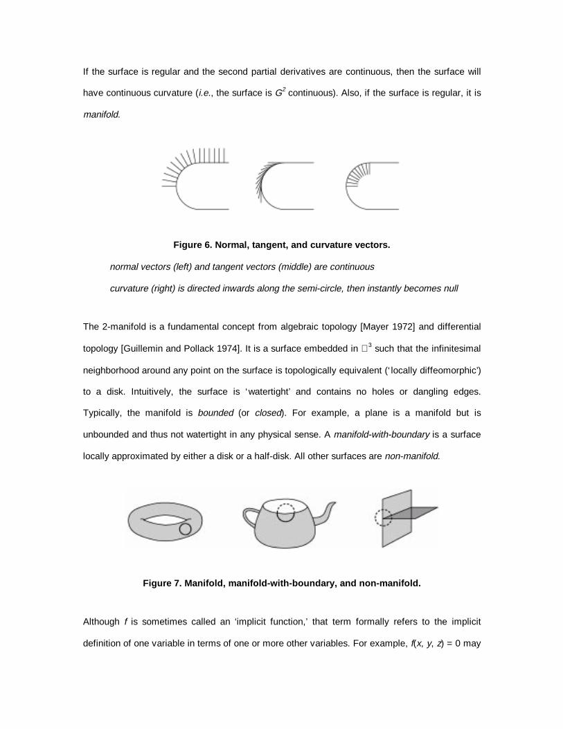
Figure 6. Normal, tangent, and curvature vectors.

normal vectors (left) and tangent vectors (middle) are continuous

curvature (right) is directed inwards along the semi-circle, then instantly becomes null

The 2-manifold is a fundamental concept from algebraic topology [Mayer 1972] and differential

topology [Guillemin and Pollack 1974]. It is a surface embedded in ℜ3 such that the infinitesimal

neighborhood around any point on the surface is topologically equivalent (‘ locally diffeomorphic’)

to a disk. Intuitively, the surface is ‘watertight’ and contains no holes or dangling edges.

Typically, the manifold is bounded (or closed). For example, a plane is a manifold but is

unbounded and thus not watertight in any physical sense. A manifold-with-boundary is a surface

locally approximated by either a disk or a half-disk. All other surfaces are non-manifold.

Figure 7. Manifold, manifold-with-boundary, and non-manifold.

Although f is sometimes called an ‘implicit function,’ that term formally refers to the implicit

definition of one variable in terms of one or more other variables. For example, f(x, y, z) = 0 may

be rewritten as f(x, y, g(x,y)) = 0. The Implicit Function Theorem gives those conditions under

which a unique g exists and is C1 continuous [Spivak 1965].

From the implicit function theorem it may be shown that for f(p) = 0, where 0 a regular value of f

and f is continuous, the implicit surface is a two-dimensional manifold [Bruce and Giblin 1992,

prop. 4.16]. The Jordan-Brouwer Separation Theorem states that such a manifold separates

space into the surface itself and two connected open sets: an infinite òutside' and a finite ‘inside'

[Guillemin and Pollack 1974].

Consider two examples for which no manifold exists. The first is simply f(p) = 0. Here, ∇f is

everywhere 0, there is no ìnside' nor òutside' and no boundary between the two. The second is

a degenerate sphere f(x, y, z) = x2+y2+z2. Here, ∇f = (2x, 2y, 2z), which is null at the origin, the

only point satisfying f; intuitively, the ìnside' is degenerate. Whether or not a surface is manifold

concerns its polygonal representation.

Polygonal Representation

For many applications it is useful to approximate an implicit surface with a mesh of triangles or

polygons (formally, a discrete set of piecewise-linear, semi-disjoint elements). For differentiable f

this is always possible because all manifold surfaces may be triangulated [Whitney 1957].

Although approximate, the mesh is a practical representation for Z(f). [Hoffmann 1993] notes the

difficulty in obtaining exact mathematical representations (parametric or implicit) for conceptually

simple surfaces such as the offset surface (a surface a fixed distance from a base surface) and

the equi-distance surface (a surface lying between two surfaces). There are simple procedural

descriptions for both of these surfaces, each readily converted to a polygonal mesh.

Mesh conversion, popularly known as polygonization, usually involves partitioning space into

convex cells (typically cubes or tetrahedra). A cell is transverse if any of its edges intersects the

implicit surface (i.e., one edge endpoint evaluates negatively, the other positively). For each

transverse edge, a surface vertex is computed (by the Intermediate Value Theorem, a point p:

f(p) = 0 must exist along a transverse edge if f is continuous). The surface vertices belonging to

the transverse edges of a cell are connected to form one or more polygons (alternatively,

patches may be produced). The edges of the polygons lie within the faces of the cell.

The order of vertex connectivity is often stored in a table of polarity configurations of the cell

corners. For the cube (8 corners) and the tetrahedron (4 corners, i.e., a three-dimensional

simplex) there are 256 and 16 possibilities, respectively. Any convex cell may be decomposed

into tetrahedra, thereby simplifying the case analysis. Any (possibly non-planar) n-sided polygon

produced may be decomposed into n+2 triangles; alternatively, n triangles can radiate from a

polygon centroid.

Figure 8. Polygonization.

A review of discrete and continuous polygonization methods is given in [Kalvin 1992]. An

analysis of implementation complexity, polygon count, and topological and geometric accuracy is

given in [Ning and Bloomenthal 1993]. Other criteria, such as the number of function

evaluations, the adaptive distribution of polygons, and visual appearance are discussed in

[Schmidt 93]. A review of discrete data methods is given in [Schroeder et al. 1996].

Software implementations typically utilize exhaustive enumeration [Mäntylä 1988], subdivision

[Bloomenthal 1988], or numerical continuation [Allgower and Georg 1990].

Exhaustive Enumeration

Exhaustive enumeration operates on a set of samples of f arranged as a regular, typically

rectilinear lattice known as a scalar grid or voxel array. The samples may be experimental, such

as CAT and MRI scans, or computed, as in simulations of fluid flow. The lattice is readily

represented by a three-dimensional memory array, which can be filled by a hardware scanner in

constant time.

Once the samples are obtained, each transverse cell is polygonized. Given c1 and c2, lattice

neighbors of opposite sign, a surface vertex v is usually is computed using linear interpolation:

v = αc1+(1−α)c2, where α = f(c2)/(f(c2)−f(c1))

This method is popularly known as ‘marching cubes’ and may be optimized for one plane of cells

at a time [Lorensen and Cline 1987]. Cells may be pre-sorted according to minimum and

maximum f; should an offset (i.e., isovalue) be applied to f, transverse cells can be quickly

identified from the sort [Wilhelms and van Gelder 1992; Laszlo 1992].

The application of marching cubes algorithms includes electron motion [Tindle 1986],

computational electromagnetics [Ambrosiano et al. 1994], polypeptide visualization [Fujii et al.

1992], biomedical visualization [Kalvin 1991], and molecular modeling [Koide et al. 1986; Doi

and Koide 1991; Doi and Koide 1992; Purvis and Culberson 1985]. Rendering and polygonization

schemes for irregular lattices, such as produced by finite element methods, are discussed in [Itoh

and Koyamada 1995].

Unlike exhaustive evaluation, subdivision and continuation operate on synthetic functions (i.e., f

may be algebraic or procedural), typically for the purpose of design [Ricci 1973]. f may be

evaluated at arbitrary locations, which allows methods such as binary sectioning to compute

surface vertex locations with arbitrary precision, unlike linear interpolation. These algorithms

seek to minimize the number of evaluations of f, which may be arbitrarily demanding to evaluate.

Subdivision

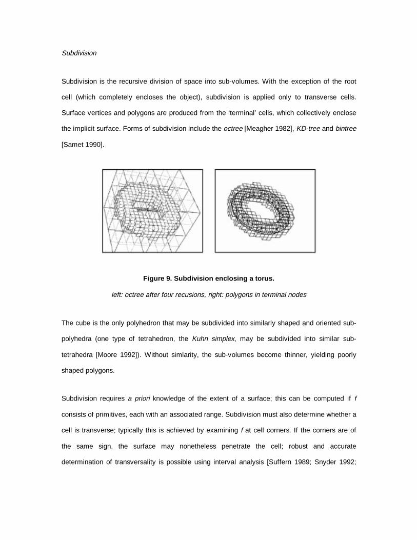
Subdivision is the recursive division of space into sub-volumes. With the exception of the root

cell (which completely encloses the object), subdivision is applied only to transverse cells.

Surface vertices and polygons are produced from the ‘terminal’ cells, which collectively enclose

the implicit surface. Forms of subdivision include the octree [Meagher 1982], KD-tree and bintree

[Samet 1990].

Figure 9. Subdivision enclosing a torus.

left: octree after four recusions, right: polygons in terminal nodes

The cube is the only polyhedron that may be subdivided into similarly shaped and oriented sub-

polyhedra (one type of tetrahedron, the Kuhn simplex, may be subdivided into similar sub-

tetrahedra [Moore 1992]). Without simlarity, the sub-volumes become thinner, yielding poorly

shaped polygons.

Subdivision requires a priori knowledge of the extent of a surface; this can be computed if f

consists of primitives, each with an associated range. Subdivision must also determine whether a

cell is transverse; typically this is achieved by examining f at cell corners. If the corners are of

the same sign, the surface may nonetheless penetrate the cell; robust and accurate

determination of transversality is possible using interval analysis [Suffern 1989; Snyder 1992;

Duff 1992], Lipschitz constants [Von Herzen and Barr 1987; Kalra and Barr 1989], or derivative

bounds [Hart 1997].

Rather than subdivide a large cell, it is possible to propagate from one small cell to another. This

is a form of numerical continuation, a class of techniques usually divided into piecewise-linear

and predictor-corrector [Allgower and Georg 1990].

Piecewise-Linear Continuation

Piecewise-linear principles (see [Coxeter 1934], [Freudenthal 1942]) have been applied to

implicit surfaces using a tetrahedral cell [Allgower and Schmidt 1985] and a cubic cell [Wyvill et

al. 1986]. Beginning with a single transverse ‘seed’ cell, new cells are propagated across

transverse faces until the entire surface is enclosed.

Because only transverse cells are generated, piecewise-linear continuation requires O(n−2)

function evaluations, where n is cell size. In comparison, exhaustive enumeration requires O(n−3)

samples. Compared with subdivision, continuation appears less prone to under-sampling.

Exhaustive enumeration yields all disjoint (and detectable) surface components. Continuation,

however, produces a single component for each seed cell; to polygonize all disjoint surface

components, continuation must be performed for each, using an appropriate seed cell.

Predictor-Corrector Continuation

Predictor-corrector methods (similar to ‘meshing’ used in numerical grid generation) apply

directly to the surface, creating elements (usually triangles or polygons) by joining an initial

surface point with additional points. New points are computed by displacement from a known

point along the tangent plane and then corrected (e.g., using Newton iteration) onto the surface

[Rheinboldt 1988]. These methods are problematic for surfaces because surface vertices are not

intrinsically ordered (unlike a one-dimensional contour), which complicates detection of global

overlap.

Adaptive Polygonization

Polygonization is a sampling process; if the spacing between samples is large with respect to

surface curvature, detail is lost. Resolution requirements may also change with viewpoint. Any

fixed sampling rate may be excessive for relatively flat regions of the surface and insufficient for

relatively curved regions. If the cell size is inversely proportional to local curvature, the resulting

adaptive polygonization minimizes polygon count while maintaining geometric accuracy [Hall and

Warren 1990]. Both subdivision and continuation may be performed adaptively [Bloomenthal

1988]. Accurate representation of non-differentiable f, however, may require explicit computation

of its singular points.

Surface refinement is an adaptive method in which a coarsely polygonized surface is followed by

subdivision of insufficiently accurate polygons. For example, if the center of a triangle is too

distant from the surface, the triangle may be split at its center, which is moved to the surface

[Allgower and Gnutzmann 1991]. Similarly, a triangle may be divided along its edges if the

divergence between surface normals at the triangle vertices is too great [Velho 1996].

Figure 10. Adaptively polygonized object.

Adaptive polygonization is also possible through the use of ‘physically-based particles’ distributed

along the implicit surface, with particle density locally proportional to surface complexity

[Figueiredo et al. 1992]. Particle location is determined by various heuristics, including the use

of the gradient of f [Bloomenthal and Wyvill 1990; Figueiredo and Gomes 1996]. During

animation, the topology of a particle-based polygonization may be maintained by operating on

those critical points at which topological change occurs [Stander and Hart 1996].

Non-Manifold Polygonization

Although a manifold-with-boundary may be specified by a continuous function, all points off the

zero set are of the same sign. Consequently, conventional polygonization fails.

Figure 11. Union, difference, and manifold-with-boundary (zero contours are dashed).

left to right: min(f1, f2), f1max(f1,f2), abs(f1)−min(0,f2)

where f1 = ||p−c1||/r1−1 and f2 = ||p−c2||/r2−1 are two circles

As suggested in [Rossignac and O'Connor 1990], a non-manifold can be implicitly represented

by extending the definition of f to be the separation between arbitrary regions of space. A

continuation method using this scheme is given in [Bloomenthal and Ferguson 1995].

Figure 12. Polygonized non-manifold.

CSG Polygonization

The primitives in constructive solid geometry (CSG) may be represented implicitly and combined

by set-theoretic Boolean operations. These operations may create hard-edged junctions that

conventional polygonizers cannot accurately approximate. A method presented in [Wyvill and

van Overveld 1997] computes surface vertices on cell edges in the usual manner, but the CSG

state at the cell corners determines whether a crease is applied to the resulting polygon.

Figure 13: Polygonized CSG objects.

courtesy Brian Wyvill and Kees van Overveld

Relation to Parametric Surfaces

Both parametric and implicit methods are well developed in computer graphics. A modern

treatment of parametric surfaces is in [Farin 1993]. Traditionally, computer graphics has favored

polynomial parametric over implicit surfaces because they are simpler to render and more

convenient for geometric operations such as computing curvature and controlling position and

tangency. Parametric surfaces are generally easier to draw, tessellate, subdivide, bound, and

navigate along [Rockwood 1989].

An implicit surface naturally describes an object’s interior, whereas a comparable parametric

description is usually piecewise. The ability to enclose volume and to represent blends of

volumes provides a straightforward (although less precise) implicit alternative to fillets, rounds,

and other ‘free-form’ parametric surfaces that require care in joining so that geometric continuity

is established along the seams [Charrot and Gregory 1984]. Consequently, animations of organic

shapes commonly employ implicit surfaces.

Figure 14. A free-form parametric surface.

Point classification (determining whether a point is inside, outside, or on a surface) is simpler

with implicit surfaces, depending only on the sign of f. This facilitates the construction of complex

objects from primitive ones [Ricci 1973], and simplifies collision detection [Sclaroff and Pentland

1991].

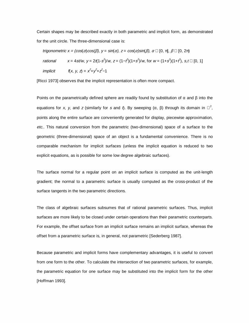
Certain shapes may be described exactly in both parametric and implicit form, as demonstrated

for the unit circle. The three-dimensional case is:

trigonometric x = (cos(α)cos(β), y = sin(α), z = cos(α)sin(β), α ∈ [0, π], β ∈ [0, 2π)

rational x = 4st/w, y = 2t(1-s2)/w, z = (1−t2)(1+s2)/w, for w = (1+s2)(1+t2), s,t ∈ [0, 1]

implicit f(x, y, z) = x2+y2+z2−1

[Ricci 1973] observes that the implicit representation is often more compact.

Points on the parametrically defined sphere are readily found by substitution of α and β into the

equations for x, y, and z (similarly for s and t). By sweeping (α, β) through its domain in ℜ2,

points along the entire surface are conveniently generated for display, piecewise approximation,

etc.. This natural conversion from the parametric (two-dimensional) space of a surface to the

geometric (three-dimensional) space of an object is a fundamental convenience. There is no

comparable mechanism for implicit surfaces (unless the implicit equation is reduced to two

explicit equations, as is possible for some low degree algebraic surfaces).

The surface normal for a regular point on an implicit surface is computed as the unit-length

gradient; the normal to a parametric surface is usually computed as the cross-product of the

surface tangents in the two parametric directions.

The class of algebraic surfaces subsumes that of rational parametric surfaces. Thus, implicit

surfaces are more likely to be closed under certain operations than their parametric counterparts.

For example, the offset surface from an implicit surface remains an implicit surface, whereas the

offset from a parametric surface is, in general, not parametric [Sederberg 1987].

Because parametric and implicit forms have complementary advantages, it is useful to convert

from one form to the other. To calculate the intersection of two parametric surfaces, for example,

the parametric equation for one surface may be substituted into the implicit form for the other

[Hoffman 1993].

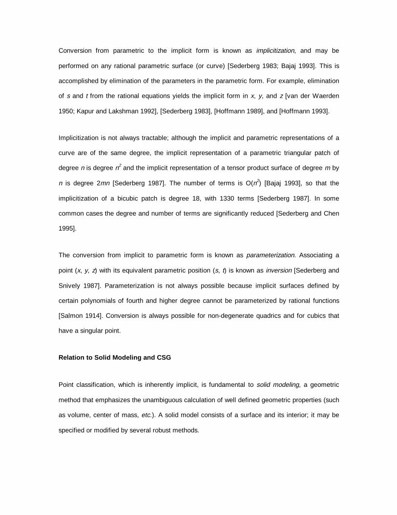
Conversion from parametric to the implicit form is known as implicitization, and may be

performed on any rational parametric surface (or curve) [Sederberg 1983; Bajaj 1993]. This is

accomplished by elimination of the parameters in the parametric form. For example, elimination

of s and t from the rational equations yields the implicit form in x, y, and z [van der Waerden

1950; Kapur and Lakshman 1992], [Sederberg 1983], [Hoffmann 1989], and [Hoffmann 1993].

Implicitization is not always tractable; although the implicit and parametric representations of a

curve are of the same degree, the implicit representation of a parametric triangular patch of

degree n is degree n2 and the implicit representation of a tensor product surface of degree m by

n is degree 2mn [Sederberg 1987]. The number of terms is O(n2) [Bajaj 1993], so that the

implicitization of a bicubic patch is degree 18, with 1330 terms [Sederberg 1987]. In some

common cases the degree and number of terms are significantly reduced [Sederberg and Chen

1995].

The conversion from implicit to parametric form is known as parameterization. Associating a

point (x, y, z) with its equivalent parametric position (s, t) is known as inversion [Sederberg and

Snively 1987]. Parameterization is not always possible because implicit surfaces defined by

certain polynomials of fourth and higher degree cannot be parameterized by rational functions

[Salmon 1914]. Conversion is always possible for non-degenerate quadrics and for cubics that

have a singular point.

Relation to Solid Modeling and CSG

Point classification, which is inherently implicit, is fundamental to solid modeling, a geometric

method that emphasizes the unambiguous calculation of well defined geometric properties (such

as volume, center of mass, etc.). A solid model consists of a surface and its interior; it may be

specified or modified by several robust methods.

The theoretical underpinnings of solid modeling are found in point-set topology: a ‘reasonable’

solid is ‘all material,’ i.e., a bounded, closed set of points in ℜ3 that is regular (free from any

dangling points, edges, or faces). Regularity is ``widely used as a characterization of reasonable

solids'' [Mäntylä 1988]. A finite, regular point-set is called an r-set [Requicha 1980], and a solid

model is usually confined to an r-set whose surface is analytic.

An initial means to specify solids was introduced in [Ricci 1973], which developed a ‘constructive

geometry’ for the purpose of defining complex shapes derived from operations, including blend,

upon simple implicit primitives (the operations, known as Comba-Ricci sums, are reviewed in

[Tavares and Gomes 1989]). A primitive solid is described by P(p) < 0 (convention of sign is not

generally observed for implicit surfaces).

The closed-form definition given in [Ricci 1973] was superceded by constructive solid geometry

(CSG), which is characterized by a ‘bottom-up’ binary tree evaluation. The leaf nodes are usually

arbitrarily placed and oriented low degree polynomial primitives (viz., the parallelepiped, sphere,

ellipsoid, cylinder, cone, and torus). The internal nodes represent regularized Boolean set-

theoretic operations (union, intersection, and difference), which are common in computer aided

design and manufacture.

Union is given as min(P1, P2); intuitively, if a point is within any sphere it evaluates negatively,

regardless of the number of surrounding spheres. Intersection is given as max(P1, P2); i.e., if a

point is outside any sphere, it evaluates positively. Difference is given by max(P1, −P2). Because

the solid model unambiguously separates inside from outside, it defines a realizable manifold

and polygonization methods typically succeed.

min and max are semi-analytic, however, as they are not everywhere differentiable. Analytic

expressions approximating union and intersection (for n functions) are given in [Ricci 1973] as:

unionα (f1, . . ., fn) = (f1−α+. . .+fn

−α)−1/α

and

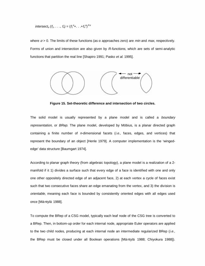
intersectα (f1, . . ., fn) = (f1α+. . .+fn

α)1/α

where α > 0. The limits of these functions (as α approaches zero) are min and max, respectively.

Forms of union and intersection are also given by R-functions, which are sets of semi-analytic

functions that partition the real line [Shapiro 1991; Pasko et al. 1995].

Figure 15. Set-theoretic difference and intersection of two circles.

The solid model is usually represented by a plane model and is called a boundary

representation, or BRep. The plane model, developed by Möbius, is a planar directed graph

containing a finite number of n-dimensional facets (i.e., faces, edges, and vertices) that

represent the boundary of an object [Henle 1979]. A computer implementation is the ‘winged-

edge’ data structure [Baumgart 1974].

According to planar graph theory (from algebraic topology), a plane model is a realization of a 2-

manifold if it 1) divides a surface such that every edge of a face is identified with one and only

one other oppositely directed edge of an adjacent face, 2) at each vertex a cycle of faces exist

such that two consecutive faces share an edge emanating from the vertex, and 3) the division is

orientable, meaning each face is bounded by consistently oriented edges with all edges used

once [Mäntylä 1988].

To compute the BRep of a CSG model, typically each leaf node of the CSG tree is converted to

a BRep. Then, in bottom-up order for each internal node, appropriate Euler operators are applied

to the two child nodes, producing at each internal node an intermediate regularized BRep (i.e.,

the BRep must be closed under all Boolean operations [Mäntylä 1988; Chiyokura 1988]).

notdifferentiable

Regularity typically disallows non-manifold objects, although support does exist for non-regular

and other free-form methods [Rossignac and Requicha 1991]. To maintain a regularized BRep at

each node, each set operation must support a multitude of geometric intersections, many of

which are difficult to implement robustly in the presence of numerical errors [Mäntylä 1988].

Either an ordered sequence of edges around each vertex or an ordered list of edges around each

face are sufficient to reproduce an adjacency graph embedded in a two-dimensional manifold

[Weiler 1986]. In other words, the topologically more complete BRep can be obtained from the

representationally simpler mesh produced by polygonization.

Relation to Algebraic Surfaces

When f is polynomial the corresponding implicit surface is an algebraic surface (also called

algebraic set). The basis of the polynomial is usually the power basis (i.e, x, x2, x3 ...) but could

be another, such as the Bernstein (used by Bézier curves and surfaces). For the purpose of

geometric modeling, coefficients are limited to the reals. The degree of an algebraic expression

is the maximum degree of its terms. When f is linear (degree 1), it describes a plane. When f is

quadratic (degree 2), it describes a quadric surface, which is an ellipsoid, sphere, cylinder, cone,

paraboloid, hyperboloid, or hyperbolic paraboloid, or is degenerate (a plane, line, or point). The

quadrics may also be expressed in trigonometric form; when exponentiated, the trigonometric

terms yield a superquadric [Barr 1981].

It may be difficult to perform geometric operations, such as surface/surface intersection, on

algebraic surfaces of degree greater than three because the degree of the resulting surface is

often very high.

The animation of algebraic surfaces is discussed in [Saupe and Ruhl 1995]. A general

development of algebraic surfaces is given in [Sederberg 1985], [Sederberg 1987], and [Bajaj

1992]. Other salient properties of algebraic surfaces are discussed in [Zariski 1935; Hoffmann

1989].

Algebraic surfaces may also be defined parametrically by three independent equations, one each

for x, y, and z. Further, the equations may be rational; that is, x = f(s, t) / g(s, t), where f and g

are polynomials (similarly for y and z). Rational polynomial parametric surfaces are a subset of

implicit algebraic surfaces; each rational parametric surface may be expressed in implicit form,

but the converse does not hold [Bajaj 1993]. A theorem by Noether states that a planar algebraic

curve f(x, y) = 0 has an equivalent rational parametric form if and only if f has a genus of 0. A

similar theorem for surfaces is provided by Castelnuovo [Zariski 1935]. All non-degenerate

quadric surfaces in implicit form may be converted to parametric form [Salmon 1914].

Algebraic surfaces may define non-manifolds. For example, the Steiner surface

(x2y2+y2z2+z2x2+xyz = 0) contains the coordinate axes, where it is singular.

Figure 16. The Steiner patch.

An algebraic surface must consist of a finite number of components, which is not the case for

transcendental functions. For example, f(x, y) = cos(x)sin(y)−1 = 0 yields zero-contours

throughout the plane.

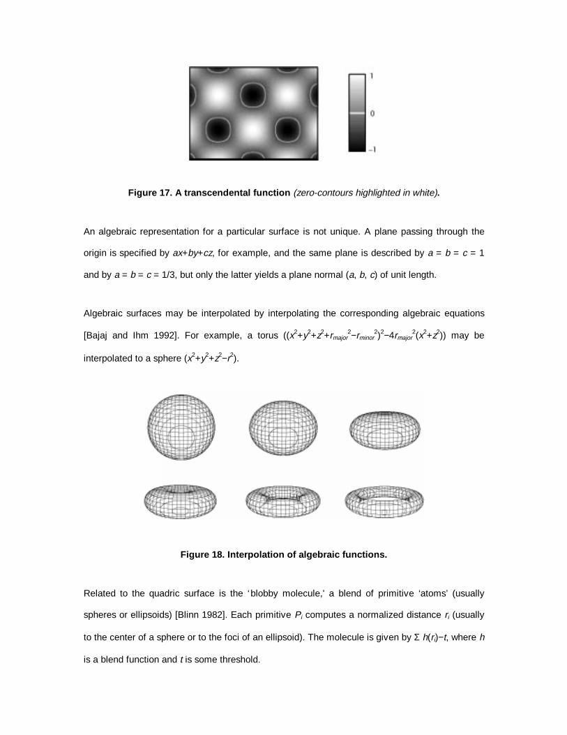
Figure 17. A transcendental function (zero-contours highlighted in white).

An algebraic representation for a particular surface is not unique. A plane passing through the

origin is specified by ax+by+cz, for example, and the same plane is described by a = b = c = 1

and by a = b = c = 1/3, but only the latter yields a plane normal (a, b, c) of unit length.

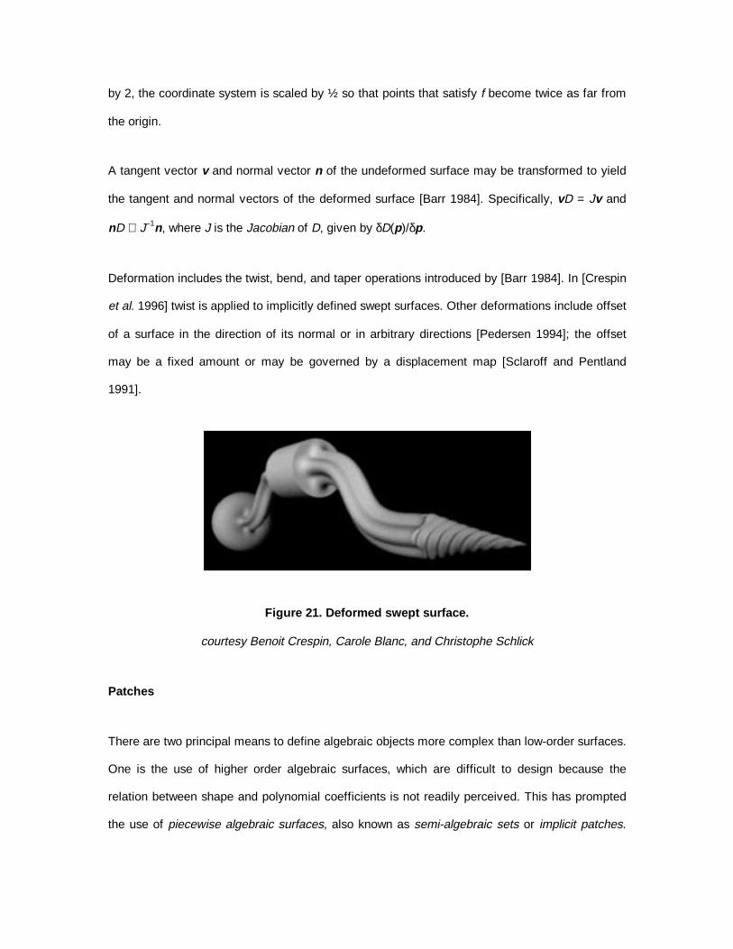
Algebraic surfaces may be interpolated by interpolating the corresponding algebraic equations

[Bajaj and Ihm 1992]. For example, a torus ((x2+y2+z2+rmajor2−rminor

2)2−4rmajor2(x2+z2)) may be

interpolated to a sphere (x2+y2+z2−r2).

Figure 18. Interpolation of algebraic functions.

Related to the quadric surface is the ‘blobby molecule,' a blend of primitive ‘atoms’ (usually

spheres or ellipsoids) [Blinn 1982]. Each primitive Pi computes a normalized distance ri (usually

to the center of a sphere or to the foci of an ellipsoid). The molecule is given by Σ h(ri)−t, where h

is a blend function and t is some threshold.

Figure 19. Contribution of a primitive P as a function of distance.

h is usually monotonic and sigmoidal. The domain rmax of h affects the primitive’s range of

influence and the shape of h determines the primitive’s radius in isolation and blending

characteristics. In [Blinn 1982] h is an exponential; in [Nishimura et al. 1985] piecewise

quadratics produce what are popularly called ‘metaballs’ and in [Wyvill et al. 1986] a sixth degree

polynomial produces ‘soft objects.’

The geometric continuity of h at rmax determines the effect of one atom on its neighbor. For

example, [Wyvill et al. 1986] gives:

h(r) = 1−(4/9)r6+(17/)9r4−(22/9)r2 for r ∈ [0, 1], 1 for r < 0, 0 for r > 1,

where r = d/R, d is distance to the primitive, and R is the range of influence of the primitive. This

may be factored into:

(r2−1)2 (9−4r2)/9

The two roots at r = 1 = rmax imply an order of continuity of 1. That is, if the influence of two

atoms overlap, the seam between the area of mutual influence and the areas influenced only by

one atom is G1 continuous. Another function due G.Wyvill is (1−r2)3, which, having three multiple

roots at r = 1, implies a G2 continuous blend [Bloomenthal 1997, chapter 5].

The union of two algebraic surfaces is usually given by the product of the corresponding

algebraic functions. Intuitively, if f is zero, then any multiple of f, including multiplication by

another function, is zero. For example, consider two spheres given by f1 = ||p−c1||−r1 and f2 =

rt

t

rmax

||p−c2||−r2, where ci and ri are the centers and radii. Each function is negative inside the sphere’s

radius and positive outside.

The multiplication f1f2 confuses the sense of inside and outside, however. That is, points that are

within both spheres as well as points beyond both spheres evaluate positively; only points within

one and only one sphere evaluate negatively. This produces internal boundaries that are difficult

to polygonize and typically undesirable in geometric design. In contrast, solid modeling operates

on volumes, rather than surfaces, and does not produce internal boundaries.

Figure 20. Algebraic (left) and set-theoretic (right) unions (zero set is highlighted in white).

The complexity of an algebraic surface can be partly understood in terms of intersections with

curves or surfaces. A generalization of Bezout’s Theorem states that an algebraic curve of

degree m intersects an algebraic surface of degree n in at most mn points (assuming no part of

the curve is common with the surface), and that the intersection of a surface of degree m with a

surface of degree n is an algebraic curve of degree mn or less [Zariski 1935]. For example, a line

may intersect an algebraic surface of degree m no more than m times; two ellipses (each of

degree 2) may intersect at no more than four points.

Deformations

An implicit surface may be defined by a deformation. A deformation D maps each point in three-

space to some new location; that is, p’ = D(p). If D is to apply to an implicit surface, the inverse

of D must be applied to the space within which the implicit surface is embedded; in other words,

fD(p) = f(D−1(p)), where fD is the deforming implicit function. For example, to scale the unit circle

f1f2 min(f1, f2)

by 2, the coordinate system is scaled by ½ so that points that satisfy f become twice as far from

the origin.

A tangent vector v and normal vector n of the undeformed surface may be transformed to yield

the tangent and normal vectors of the deformed surface [Barr 1984]. Specifically, vD = Jv and

nD ∝ J−1n, where J is the Jacobian of D, given by δD(p)/δp.

Deformation includes the twist, bend, and taper operations introduced by [Barr 1984]. In [Crespin

et al. 1996] twist is applied to implicitly defined swept surfaces. Other deformations include offset

of a surface in the direction of its normal or in arbitrary directions [Pedersen 1994]; the offset

may be a fixed amount or may be governed by a displacement map [Sclaroff and Pentland

1991].

Figure 21. Deformed swept surface.

courtesy Benoit Crespin, Carole Blanc, and Christophe Schlick

Patches

There are two principal means to define algebraic objects more complex than low-order surfaces.

One is the use of higher order algebraic surfaces, which are difficult to design because the

relation between shape and polynomial coefficients is not readily perceived. This has prompted

the use of piecewise algebraic surfaces, also known as semi-algebraic sets or implicit patches.

Each surface piece is low order and spans a single (usually tetrahedral) cell within a spatial

partitioning.

Patch shape is typically specified by a grid of control points that deforms the enclosed space

according to a Bernstein polynomial (although other bases, such as the Bspline, can be used)

[Sederberg 1985]. This method is central to free-form deformation, a technique to manipulate

solid models and algebraic surfaces (and widely applied to other geometric objects, such as

curves, patches, and polygonal meshes) [Sederberg and Parry 1986].

As with parametric patches, the algebraic patches must be carefully joined to maintain geometric

continuity along their boundaries. Depending on the application, the cells can be recursively

subdivided to adapt to local curvature while maintaining C1 or C2 continuity across the patch

boundaries. [Warren 1992] provides a method to generate implicit patches from a polygonal

mesh. At each mesh location the derivatives of the patches are averaged to improve continuity

along the seams.

Algebraic patches provide a compact and highly continuous surface representation; they are

reviewed in [Bajaj 1993].

Procedural Methods

As observed in [Ricci 1973], f may be procedural, i.e., any arbitrary process that computes a real

value given a point in space. The process may use mathematical functions, conditionals, tables,

randomness, etc. The procedurally defined ‘hypertexture’ [Perlin and Hoffert 1989] is an implicit

surface derived from stochastically varied densities within a volume. Iterative and fractal

surfaces may also be procedurally implicit. Procedural methods are not generally expressible in

closed form, however, and so cannot be understood with analytic geometry. Further, their

interactive specification is not well understood, with few examples [Nelson 1985; Fowler et al.

1992].

Figure 22. Iteratively computed slice through quadratic Julia sets.

courtesy John Hart and Greg Turk

Voxels may be employed as a procedural design method. For example, accumulation modeling

disperses values along some path, iteratively to neighboring array elements [Smith 1982;

Williams 1990; Greene 1989]. This can be computationally demanding, but allows the simulation

of developmental processes. Other uses include smoothing [Galyean and Hughes 1991;

Bloomenthal 1997, chapter 7; Wilhelms 1997] and volume-based metamorphosis [Hughes 1992;

Lerios et al. 1995].

Figure 23. Voxel-based model of tree roots and obstacles.

courtesy Ned Greene

As with any sampling process, the Sampling Theorem [see Oppenheim and Schafer 1975]

requires that each voxel represent a filtered volume (i.e., a weighted average of the

neighborhood surrounding the sample point); otherwise, aliasing may result [Wang and Kaufman

1994].

Skeletal Methods

The skeleton, a standard CAD representation, may be used as a procedural element of implicit

design. It typically consists of a hierarchical set of ‘limbs’ that each generate an implicit primitive.

Each limb may support one or more descendent limbs. The relationship between child and

parent limbs is usually given as an affine transformation that specifies size and orientation

[O'Donnell and Olson 1981; Reeves 1990].

With modern input and display devices, it is feasible to manipulate and display in real-time

complex skeletons and associated implicit primitives [Bloomenthal and Wyvill 1990; Witkin and

Heckbert 1994]. Shapes intermediate to key poses typically rely on rigid body rotation at the

skeletal joints, as other schemes appear unnatural.

Figure 24. Interpolations of implicit contours generated by skeletons S1 and S2.

top to bottom: algebraic interpolation, interpolation of segment endpoints, interpolation of

segment angle

f may be given as the union of primitives or, for a more smooth result, as a blend. For example,

given two primitives P1(p) and P2(p), f = B(P1, P2) = 0, where B is some blend function, such as

1−(1−P1)2−(1−P2)

2. Various blends are examined in [Rockwood 1989], [Warren 1989] and

[Hoffman and Hopcroft 1985]; [Woodwark 1986] provides a survey.

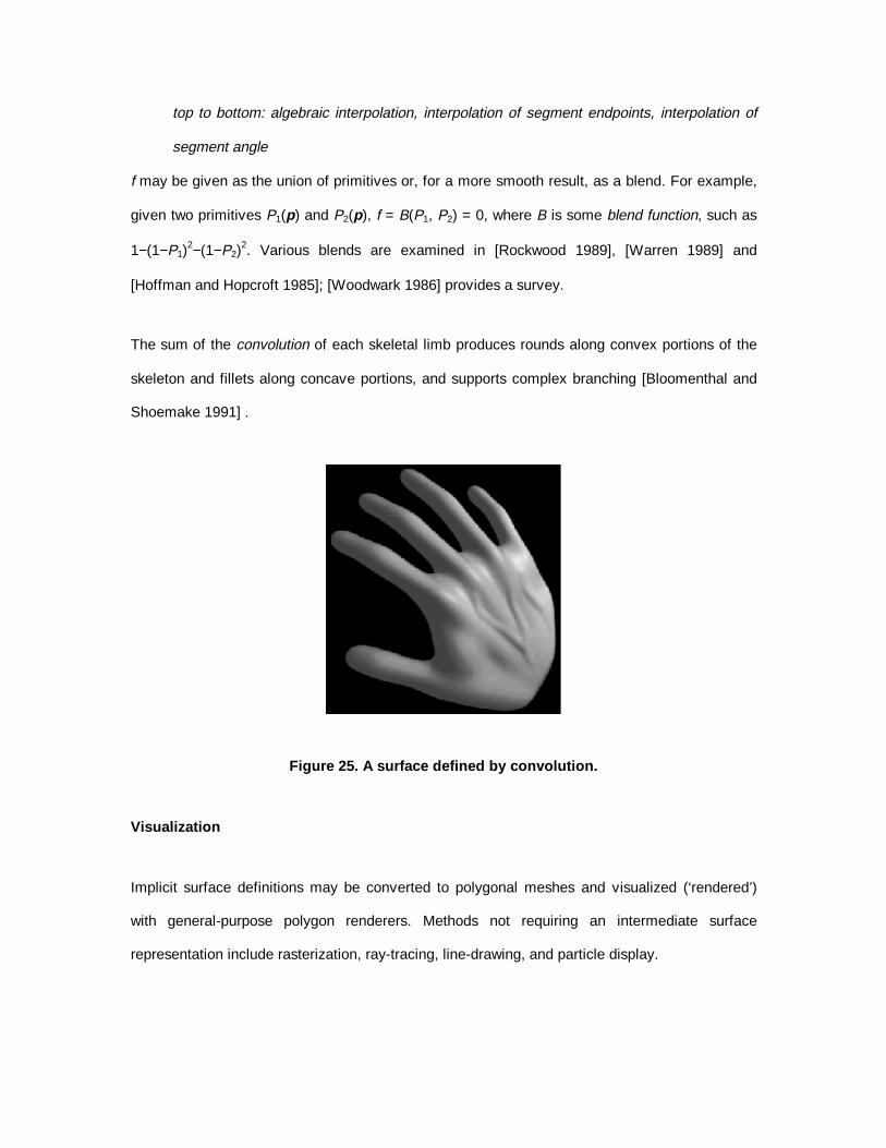
The sum of the convolution of each skeletal limb produces rounds along convex portions of the

skeleton and fillets along concave portions, and supports complex branching [Bloomenthal and

Shoemake 1991] .

Figure 25. A surface defined by convolution.

Visualization

Implicit surface definitions may be converted to polygonal meshes and visualized (‘rendered’)

with general-purpose polygon renderers. Methods not requiring an intermediate surface

representation include rasterization, ray-tracing, line-drawing, and particle display.

Incremental scan-line methods (‘rasterization’) may be applied to quadric surfaces [Goldstein

and Nagel 1971; Levin 1976; Blinn 1982; Mittelman 1983; Davis et al. 1968; Bronsvoort 1990;

van Kleij 1993]. Rasterization of implicitly defined curves is discussed in [Taubin 1994].

Implicit surfaces may be ray-traced directly from f, assuming the intersection of each ray with the

implicit surface is computable. General methods include a spatial partitioning (such as an octree)

that reduces the problem to the intersection of a ray with terminal cells of the partitioning [Roth

1982]. For each terminal cell, assuming there is a positive intersection and a negative

intersection with the ray, the ray-surface intersection may be computed by binary sectioning,

regula falsi, or some other technique; for low-degree algebraic surfaces, analytic methods may

be used [Roth 1982]. Performance may be improved by application of interval analysis [Mitchell

1990], with specific optimizations reported for metaballs [Nishita and Nakamae 1994]. Algebraic

surfaces may be ray-traced by symbolic methods that are particularly efficient and accurate

[Hanrahan 1983]. Implicit surfaces generally appear simpler to ray-trace than parametric patches

[Kajiya 1982].

Figure 26. A ray-traced implicit surface.

An alternative to shaded imagery is the contour-line drawing, accomplished by intersecting an

implicit surface with a series of planes, each perpendicular to the line of sight and receding from

the viewpoint [Ricci 1973]. For each plane the zero-contour is drawn, excepting those parts

obscured by previously drawn contours. Contour-line drawings are particularly useful for

engineering applications [Forrest 1979]. Like ray-tracing, the technique may be optimized using a

spatial partitioning.

Figure 27. A contour line drawing.

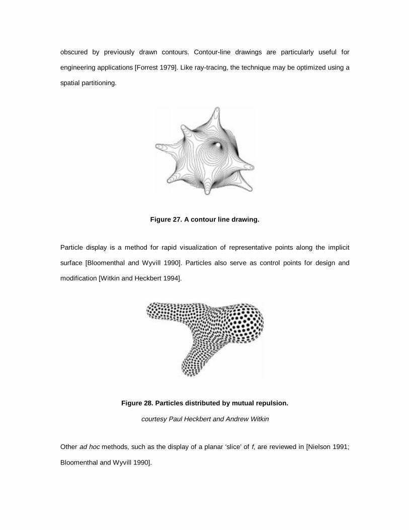
Particle display is a method for rapid visualization of representative points along the implicit

surface [Bloomenthal and Wyvill 1990]. Particles also serve as control points for design and

modification [Witkin and Heckbert 1994].

Figure 28. Particles distributed by mutual repulsion.

courtesy Paul Heckbert and Andrew Witkin

Other ad hoc methods, such as the display of a planar ‘slice’ of f, are reviewed in [Nielson 1991;

Bloomenthal and Wyvill 1990].

When solid material is of interest, an entire volume may be rendered using volume visualization,

which models light attenuation through an optical medium and is generally applied to an array of

samples of f [Drebin et al. 1988; Upson and Keeler 1988; Sabella 1988; Levoy 1988], with

variations concerned with performance [Max et al. 1990; Hanrahan 1990; Westover 1989] and

ray-tracing [Kajiya and Von Herzen 1984]. Some methods employ partial shading of estimated

surfaces within the volume [Drebin et al. 1988; Gallagher and Nagtegaal 1989]. Volume

visualization is normally an orthographic projection of a regular, affinely transformed grid;

alternative methods are considered in [Garrity 1990; Novins et al. 1990].

Photorealistic image generation requires considerable computation, encouraging the use of

efficient structures such as hierarchical detail. Hierarchical detail may be added to implicit

surfaces by applying minute geometric features to simpler, underlying shapes [Sclaroff and

Pentland 1991]; this may be implemented as a displacement [Cook 1984; Pedersen 1994], as an

operation within a procedural definition, or as functional composition from ℜ3 to ℜ3.

Figure 29. Detail as implicit composition (color-mapped to emphasize contours).

left: a(p) is a vertical gradient; middle: b(a(p)) is a smooth modification to a

right: f(p) = c(b(a(p))) provides fine detail

Alternatively, detail may be added to a polygonized implicit surface via texture synthesis [Turk

1991; Witkin and Kass 1992] or via general texture parameterization, i.e., uv-coordinate

assignment [Gagalowicz 1985; Turk 1992; Opitz and Pottmann 1994]. A parameterization free of

singularities does not necessarily exist for a given surface, and this can complicate the creation

of a realistic texture mapping. A general approach to provide uv-parameterizations for implicit

surfaces is presented in [Pedersen 1995], which observes that the implicit representation

overcomes several limitations of patch-based interactive texture painting.

Figure 30. UV-coordinate assignment governed by underlying skeleton.

left: texture coordinates, right: rendered surface

Solid texture (see [Perlin 1995; Peachey 1985]) may also be applied to implicit surfaces [Wyvill

et al. 1987]. Such texture relies on surface position not parameterization, and creates the

appearance of an object carved from, rather than covered by, a material.

Other Applications

The most common techniques for implicit modeling presently include algebraic surfaces, implicit

patches, CSG, and sums of skeletal primitives.

Implicit methods are also useful in surface reconstruction from unorganized surface points

through the use of algebraic sums [Muraki 1991; Bittar et al. 1995], the use of implicitly defined

distance to planes tangential to the surface points [Hoppe et al. 1992], or the use of algebraic

patches [Moore and Warren 1991; Bajaj 1992; Bailey et al. 1991]. Techniques to extract an

implicit surface from laser range data are given in [Bajaj et al. 1995; Curless and Levoy 1996].

Other applications include the construction of the medial axis [Bloomenthal and Lim 1999].

Outstanding issues related to implicit surface design and visualization include improved

parameterization and texturing, hardware support for visualization, and improved control of

shape.

Implicit surfaces constitute an evolving subject of considerable breadth and depth. This brief

review cannot fully cover the subject but has, hopefully, provided insight into the properties and

applications of implicit surfaces.

References

E.Allgower, K.Georg, Numerical Continuation Methods, an Introduction, Springer-Verlag, 1990

(series in Computational Mathematics, v. 13).

E.Allgower, S.Gnutzmann, Simplicial Pivoting for Mesh Generation of Implicitly Defined

Surfaces, Computer-Aided Geometric Design, 8:4, Oct. 1991, pp. 305-25.

E.Allgower, P.Schmidt, An Algorithm for Piecewise-Linear Approximation of an Implicitly Defined

Manifold, SIAM J. Numerical Analysis, 22:2, pp. 322-346, 1985.

J.Ambrosiano, S.Brandon, R.Löhner, C.DeVore, Electromagnetics via the Taylor-Galerkin Finite

Element Method on Unstructured Grids, J. Computational Physics, v. 110, pp. 310-319, 1994.

B.Bailey, C.Bajaj, M.Fields, The Vaidak Medical Imaging and Model Reconstruction Toolkit,

tech. report CSD-TR-91-066, Purdue University, 1991.

C.Bajaj, Surface Fitting with Implicit Algebraic Surface Patches, in Topics in Surface Modeling,

H. Hagen (ed.), pp. 23-52, SIAM Publications, 1992.

C.Bajaj, The Emergence of Algebraic Curves and Surfaces in Geometric Design, in Directions in

Geometric Computing, R. Martin (ed.), pp. 1-29, Information Geometers Press, UK, 1993.

C.Bajaj, I.Ihm, Algebraic Surface Design with Hermite Interpolation, ACM Proc. on Graphics,

11:1, pp. 61-91, Jan. 1992.

C.Bajaj, J.Chen, G.Xu, Free-Form Modeling with C2 Quintic A-Patches, 4 th SIAM Conf. on

Geometric Design, Sept. 1995.

A.Barr, Superquadrics and Angle-Preserving Transformations, IEEE Computer Graphics and

Applications, 1:1, Jan. 1981.

A.Barr, Global and Local Deformations of Solid Primitives, Computer Graphics, 18:3, pp. 21-30

(Proc. SIGGRAPH 84).

B.Baumgart, Geometric Modeling for Computer Vision, Ph.D. dissertation, Stanford University,

1974.

E.Bittar, N.Tsingos, M-P.Gascuel, Automatic Reconstruction of Unstructured 3D Data:

Combining Medial Axis and Implicit Surfaces, Computer Graphics Forum, 14:3, Netherlands.

J.Blinn, A Generalization of Algebraic Surface Drawing, ACM Trans. Graphics, 1:3, Jul. 1982,

pp. 135-256.

J.Bloomenthal, Polygonization of Implicit Surfaces, Computer Aided Geometric Design, 5:4,

Nov. 1988, pp. 341-355.

J.Bloomenthal (ed.), Introduction to Implicit Surfaces, Morgan Kaufmann, 1997.

J.Bloomenthal, K.Ferguson, Polygonization of Non-Manifold Surfaces, Computer Graphics, pp.

309-316 (Proc. SIGGRAPH 95).

J.Bloomenthal, C.Lim, Skeletal Methods of Shape Manipulation, Shape Modeling Int’l, Aizu-

Wakamatsu, Japan, 1999.

J.Bloomenthal, K.Shoemake, Convolution Surfaces, Computer Graphics 25:4, 1991 (Proc.

SIGGRAPH), pp. 251-256.

J.Bloomenthal, B.Wyvill, Interactive Techniques for Implicit Modeling, Computer Graphics, 24:2,

Mar. 1990, pp. 109-116.

W.Bronsvoort, Direct Display Algorithms for Solid Modeling, Jun. 1990, Ph.D. dissertation, Delft

University of Technology.

J.Bruce, P.Giblin, Curves and Singularities, Cambridge University Press, 1992.

P.Charrot, J.Gregory, A Pentagonal Surface Patch for Computer-Aided Geometric Design,

Computer-Aided Geometric Design, 1:1, 1984, pp. 87-94.

H.Chiyokura, Solid Modeling with Designbase, Addison-Wesley, 1988.

R.Cook, Shade Trees, Computer Graphics, 18:3, 1984, pp. 223-230 (Proc. SIGGRAPH 84).

H.Coxeter, Regular Polytopes. Macmillan, 1963.

B.Crespin, C.Blanc, C.Schlick, Implicit Sweep Objects, Computer Graphics Forum, 15:3, 1996,

pp. 165-174.

B.Curless, M.Levoy, A Volumetric Method for Building Complex Models from Range Images,

Computer Graphics, 1996, pp. 303-312 (Proc. SIGGRAPH 96).

J.Davis, R.Nagel, W.Guber, A Model Making and Display Technique for 3-D Pictures, Proc. 7th

Annual Meeting of UAIDE, 1968, pp. 47-72.

J.deGomes, L.Velho, Implicit Objects in Computer Graphics, Monografias de Matematica No.

53, Instituto de Matematica Pura e Aplicado, Rio de Janeiro, 1992.

L.deFigueiredo, J.deMiranda Gomes, D.Terzopoulos, L.Velho, Physically-Based Methods for

Polygonization of Implicit Surfaces, Proc.. Graphics Interface 92, pp. 250-257.

L.deFigueiredo, J.deMiranda Gomes, Sampling Implicit Objects with Physically-based Particle

Systems, Computers and Graphics, 20:3, 1996, pp. 363-375.

R.Drebin, L.Carpenter, P.Hanrahan, Volume Rendering, Computer Graphics, 1988, pp. 65-74


G.Farin, Curves and Surfaces for Computer-Aided Geometric Design: A Practical Guide,

Academic Press, 1993.

J.Foley, A.vanDam, S.Feiner, J.Hughes, Computer Graphics, Principles and Practice, Addison-

Wesley, 1992.

A.Forrest, On the Rendering of Surfaces, Computer Graphics, 13:2, 1979, pp. 253-259 (Proc.

SIGGRAPH 79).

D.Fowler, P.Prusinkiewicz, J.Battjes, A Collision-Based Model of Spiral Phyllotaxis, Computer

Graphics, 26:2, 1992, pp. 361-368 (Proc. SIGGRAPH 92).

I.Fujii, Y.Morimoto Y.Higuchi, N.Yasuoka, A Polypeptide Model-building Program for a Graphics

Workstation, J. Molecular Graphics, 10:3, Sept. 1992, pp 185-189.

R.Gallagher, J.Nagtegaal, An Efficient 3D Visualization Technique for Finite Element Models

and Other Coarse Volumes, Computer Graphics, 23:4, 1989, pp. 185-194 (Proc. SIGGRAPH

89).

A.Gagalowicz, S.deMa, Model Driven Synthesis of Natural Textures for 3D Scenes,

Eurographics 85, C.Vandoni (ed.), Elsevier Science, 1985.

T.Galyean, J.Hughes, Sculpting: An Interactive Volumetric Modeling Technique, Computer

Graphics, 25:4 1991, pp. 267-274 (Proc. SIGGRAPH 91).

M.Garrity, Raytracing Irregular Volume Data, Computer Graphics, 24:5, pp. 35-40, Nov. 1990.

R.Goldstein, R.Nagel, 3D Visual Simulation, Simulation, 16:1, 1971, pp. 25-31.

N.Greene, Voxel Space Automata: Modeling with Stochastic Growth Processes in Voxel Space,

Computer Graphics, 23:4, 1989, pp. 175-184 (Proc. SIGGRAPH 89).

V.Guillemin, A.Pollack, Differential Topology, Prentice-Hall, 1974.

M.Hall, J.Warren, Adaptive Polygonalization of Implicitly Defined Surfaces, IEEE Computer

Graphics and Applications, 10:6, Nov. 1990 pp. 33-42.

P.Hanrahan, Ray Tracing Algebraic Surfaces, Computer Graphics, 17:3, 1983, pp. 83-90 (Proc.

SIGGRAPH 83).

P.Hanrahan, Three-Pass Affine Transforms for Volume Rendering), Computer Graphics, 24:5,

pp. 71-78, 1990 (Proc. Workshop on Volume Visualization 1990).

J.Hart, Sphere-Tracing: a Geometric Method for the Antialiased Ray Tracing of Implicit Surfaces,

The Visual Computer, 12:10, 1997, pp. 527-545.

M.Henle, A Combinatorial Introduction to Topology, W.H. Freeman, 1979.

C.Hoffmann, Implicit Curves and Surfaces in Computer Aided Geometric Design, IEEE

Computer Graphics and Applications, 13:1, Jan. 1993, pp. 79-88.

C.Hoffmann, Geometric and Solid Modeling, an Introduction, Morgan Kaufmann, 1989.

C.Hoffmann, J.Hopcroft, The Potential Method for Blending Surfaces and Corners, in

Geometric Modeling, G.Farin (ed.), SIAM, 1987.

H.Hoppe, T.DeRose, T.DuChamp, J.McDonald, W.Stuetzle, Surface Reconstruction from

Unorganized Points, Computer Graphics, 26:2, 1992, pp. 71-78 (Proc. SIGGRAPH 92).

J.Hughes, Scheduled Fourier Volume Morphing, Computer Graphics, 26:2, 1992, pp. 43-46


T.Itoh, K.Koyamada, Automatic Isosurface Propagation Using an Extrema Graph and Sorted

Boundary Cell Lists, IEEE Trans. Visualization and Computer Graphics, 1:4, 1995, pp. 319-327.

J.Kajiya, B.Von Herzen, Ray Tracing Volume Densities, Computer Graphics, 18:3, 1984, pp.


A.Kalvin, Segmentation and Surface-based Modeling of Objects in 3D Biomedical Images,

Courant Inst. of Math. Sciences, Ph.D. dissertation, 1991.

A.Kalvin, A Survey of Algorithms for Constructing Surfaces from 3D Volume Data, IBM

Research Report RC 17600, Jan. 1992.

D.Kalra, A.Barr, Guaranteed Ray Intersections with Implicit Surfaces, Computer Graphics, 23:4,

1989, pp. 297-306 (Proc. SIGGRAPH 89).

J.Kajiya, Ray Tracing Parametric Patches, Computer Graphics, 16:3, 1982, pp. 245-254 (Proc.

SIGGRAPH 82).

D.Kapur, Y.Lakshman, Elimination Methods: An Introduction, in Donald, Kapur, Mundy (eds.),

Symbolic and Numerical Computation: An Integration, Academic Press, 1992.

A.Koide, A.Doi, K.Kajioka, Polyhedral Approximation Approach to Molecular Orbital Graphics, J.

Molecular Graphics, 4:3, 1986.

M.Laszlo, Fast Generation and Display of Iso-Surface Wireframes, Computer Vision Graphics

and Image Processing, 54:6, pp. 473-483, 1992.

A.Lerios, C.Garfinkle, M.Levoy, Feature-Based Volume Metamorphosis, Computer Graphics,

1995, pp. 449-456 (Proc. SIGGRAPH 95).

J.Levin, A Parametric Algorithm for Drawing Pictures of Solid Objects Bounded by Quadric

Surfaces, C. ACM, 19:11, pp. 555-563, Nov. 1976.

M.Levoy, Display of Surfaces from Volume Data, IEEE Computer Graphics and Applications,

8:3, 1988, pp. 29-37.

W.Lorensen, H.Cline, Marching Cubes: a High Resolution 3D Surface Construction Algorithm,

Computer Graphics, 21:4, 1987, pp. 163-169 (Proc. SIGGRAPH 87).

N.Max, P.Hanrahan, R.Crawfis, Area and Volume Coherence for Efficient Visualization of 3D

Scalar Functions, Computer Graphics, 24:5, Nov. 1990, pp. 27-33, (Proc. Workshop on Volume

Visualization, Dec. 1990).

J.Mayer, Algebraic Topology, Prentice-Hall, 1972.

M.Mäntylä, An Introduction to Solid Modeling, Computer Science Press, 1988.

D.Meagher, Geometric Modeling Using Octree Encoding, Computer Graphics and Image

Processing 19:2, June 1982.

D.Mitchell, Robust Ray Intersection with Interval Arithmetic, Proc. Graphics Interface 90, pp. 68-

74, May 1990.

P.Mittelman, Computer Graphics at MAGI, Computer Graphics 83, Online Publications, UK, pp.

291-301.

D.Moore, Subdividing Simplices, in D.Kirk (ed.), Graphics Gems III, Academic Press, 1992.

D.Moore, J.Warren, Adaptive Mesh Generation II: Packing Solids, Rice University technical

report TR90-139, Mar. 1991.

S.Muraki, Volumetric Shape Description of Range Data Using Blobby Model, Computer


G.Nelson, Juno, a Constraint-Based Graphics System, Computer Graphics, 19:3, 1985, pp. 235-

243 (Proc. SIGGRAPH 85).

G.Nielson, B.Hamann, The Asymptotic Decider: Resolving the Ambiguity in Marching Cubes,

Proc. Visualization 91, Oct. 1991, pp. 83-91, G.Nielson, L.Rosenblum (eds.).

P.Ning, J.Bloomenthal, An Evaluation of Implicit Surface Tilers, IEEE Computer Graphics and

Applications, 13:6, Nov. 1993, pp. 33-41.

H.Nishimura, M.Hirai, T.Kawai, T.Kawata, I.Shirakawa, K.Omura, Object Modeling by

Distribution Function and a Method of Image Generation, Trans. Inst. Electronics and

Communication Engineers of Japan, 1985, J68-D:4, pp. 718-725 (in Japanese).

T.Nishita, E.Nakamae, A Method for Displaying Metaballs by Using Bezier Clipping, Computer

Graphics Forum, v. 13 (Proc. Eurographics 94), Sept. 1994, pp. C271-C280.

K.Novins, F.Sillion, D.Greenberg, An Efficient Method for Volume Rendering using Perspective

Projection, Computer Graphics, 24:5, Nov. 1990, pp. 95-102 (Proc. Workshop on Volume

Visualization, Dec. 1990).

T.O’Donnell, A.Olson, GRAMPS: A Grapics Language Interpreter for Real-Time, Interactive,

Three-Dimensional Picture Editing and Animation, Computer Graphics, 15:3, 1981, pp. 133-142


K.Opitz, H.Pottmann, Computing Shortest Paths on Polyhedra: Applications in Geometric

Modeling and Scientific Visualization, Int’l J. Computational Geometry and Applications, 4:2,

1994, pp. 165-178.

A.Oppenheim, R.Schafer, Digital Signal Processing, Prentice Hall, 1975.

A.Pasko, V.Adzhiev, A.Sourin, V.Savchenko, Function Representation in Geometric Modeling:

Concepts, Implementation and Applications, The Visual Computer, 11: 8, 1995, pp. 429-446.

D.Peachey, Solid Texturing of Complex Surfaces, Computer Graphics, 19:3, 1985, pp. 276-286


H.Pedersen, Displacement Mapping Using Flow Fields, Computer Graphics, 1994, pp. 279-286


H.Pedersen, Decorating Implicit Surfaces, Computer Graphics, 1995, pp. 291-300 (Proc.

SIGGRAPH 95).

K.Perlin, An Image Synthesizer, Computer Graphics, 19:3, 1985, pp. 287-296 (Proc. SIGGRAPH

85).

K.Perlin, E.Hoffert, Hypertexture, Computer Graphics, 23:4, 1989, pp. 253-262 (Proc.

SIGGRAPH 89).

W.Reeves, E.Osby, The MENV Modeling and Animation Environment, J. Visualization and

Computer Animation, 1:1, 1990.

W.Rheinboldt, On the Computation of Multi-Dimensional Solution Manifolds of Parameterized

Equations, Numerische Mathematik, v. 53, pp. 165-182, 1988.

A.Requicha, Representations for Rigid Solids: Theory, Methods, and Systems, Computing

Surveys 12:4, Dec. 1980, pp. 437-464.

A.Ricci, A Constructive Geometry for Computer Graphics, The Computer J., 16:2, May 1973, pp.

157-160.

J.Rossignac, M.O’Connor, SGC: a Dimension-Independent Model for Pointsets with Internal

Structures and Incomplete Boundaries, Geometric Modeling for Product Engineering, Elsevier

Science, 1990.

J.Rossignac, A.Requicha, Constructive Non-Regularized Geometry, in Beyond Solid Modeling,

special edition of Computer Aided Design, 1991.

A.Rockwood, The Displacement Method for Implicit Blending Surfaces in Solid Models. ACM

ACM Trans. on Graphics, 8:4, Oct. 1989, pp. 279-297.

S.Roth, Ray Casting as a Method for Solid Modeling. Computer Graphics and Image Processing,

18:2, Feb. 1982, pp. 109-144.

P.Sabella, A Rendering Algorithm for Visualizing 3D Scalar Fields, Computer Graphics, 22:4,

1988, pp. 51-58 (Proc. SIGGRAPH 88).

G.Salmon, A Treatise on the Algebraic Geometry of Three Dimensions, 1:2, R.Rogers (ed.),

Chelsea Publishing, 1914.

H.Samet, Design and Analysis of Spatia Data structures, Addison-Wesley, 1990.

M.Schmidt, Cutting Cubes: Visualizing Implicit Surfaces by Adaptive Polygonization, The Visual

Computer, 10:2, 1993, pp. 101-115.

D.Saupe, M.Ruhl, Animation of Algebraic Surfaces, Proc. Visual Mathematics, Berlin, June 1995

(Int’l Workshop on Visualization and Mathematics).

S.Sclaroff, A.Pentland, Generalized Implicit Functions for Computer Graphics, Computer


W.Schroeder, K.Martin, W.Lorensen, The Visualization Toolkit, An Object-Oriented Approach To

3D Graphics, Prentice Hall, 1996.

T.Sederberg, Implicit and Parametric Curves and Surface for Computer-Aided Geometric

Design, Ph.D. dissertation, Purdue University, 1983.

T.Sederberg, Piecewise Algebraic Surface Patches, Computer Aided Geometric Design, v. 2,

1985, pp. 53-59.

T.Sederberg, Algebraic Geometry for Surface and Solid Modeling, in Geometric Modeling:

Algorithms and Trends, G. Farin (ed.), SIAM Press, 1987.

T.Sederberg, F.Chen, Implicitization using Moving Curves and Surfaces, Computer Graphics

Proc., 1995, pp. 301-308 (Proc. SIGGRAPH 95).

T.Sederberg, J.Snively, Parameterizing Cubic Algebraic Surfaces, in The Mathematics of

Surfaces II, R.Martin (ed.), Oxford University Press, 1987, pp. 299--320.

T.Sederberg, S.Parry, Free-Form Deformation of Solid Geometric Models, Computer Graphics,

20:4, 1986, pp. 151-160 (Proc. SIGGRAPH 86).

V.Shapiro, Real Functions for Representation of Rigid Solids, Cornell University technical report

TR 91-1245, Nov. 1991.

A.Smith, Plants, Fractals, and Formal Languages, Computer Graphics, 18:3, 1984 (Proc.

SIGGRAPH 84).

J.Snyder, Interval Analysis for Computer Graphics, Computer Graphics, 26:2, 1992, pp. 121-130


M.Spivak, Calculus on Manifolds, Addison-Wesley, 1965.

B.Stander, J.Hart. Guaranteeing the Topology of an Implicit Surface Polygonization. Computer


K.Suffern, Recursive Space Subdivision Techniques for Rendering Implicit Surfaces, Proc.

Australian Conf. on Computer Graphics, 1989, pp 239-250.

G.Taubin, Distance Approximations for Rasterizing Implicit Curves, ACM Trans. on Graphics,

13:1, Jan. 1994, pp. 3-42.

G.Tavares, J.deGomes, Concordance Operations for Implicitly-Defined Manifolds, Proc. SIAM

Conference on Geometric Design, 1989, SIAM Press.

G.Tindle, Fermi Surface Display, Computers and Graphics, 10:1, 1986, pp 77-79.

G.Turk, Generating Textures on Arbitrary Surfaces using Reaction Diffusion, Computer


G.Turk, Re-Tiling Polygonal Surfaces, Computer Graphics, 26:2, p. 55-64 (Proc. SIGGRAPH

92).

C.Upson, M.Keeler, V-Buffer: Visible Volume Rendering, Computer Graphics, 22:4, 1988, pp.


B.van der Waerden, Modern Algebra, v. 1 and 2, Frederick Publishing, 1950.

R.van Kleij, Display of Solid Models with Quadratic Surfaces, Ph.D. dissertation, Delft University

of Technology, 1993.

L.Velho, Simple and Efficient Polygonization of Implicit Surfaces, J. Graphics Tools, 1:1, 1996,

pp. 5-24.

B.Von Herzen, A.Barr, Accurate Triangulations of Deformed, Intersecting Surfaces, Computer

Graphics 21:4, 1987 (Proc. SIGGRAPH 87).

S.Wang, A.Kaufman, Volume-Sampled 3D Modeling, IEEE Computer Graphics and

Applications, Sept. 1994, 14:5, pp. 26-32.

J.Warren, Blending Algebraic Surfaces, ACM Transactions on Graphics 8:4, Oct. 1989,

pp. 263-278.

J.Warren, Free-Form Blending: a Technique for Creating Piecewise Implicit Surfaces, Topics in

Surface Modeling, H.Hagen (ed.), SIAM Press, 1992, pp. 3-21.

K.Weiler, Topologoical Structures for Geometric Modeling, Ph.D. dissertation, Rensselaer

Polytechnic Institute, 1986.

L.Westover, Interactive Volume Rendering, Proc. Chapel Hill Workshop on Volume

Visualization, May 1989, pp. 9-16.

H.Whitney, Elementary Structure of Real Algebraic Varieties, Annals of Mathematics 66:3, pp.

545-556, 1957.

J.Wilhelms, Animals with Anatomy, IEEE Computer Graphics and Applications, 17:3, May 1997.

J.Wilhelms, A.van Gelder, Octrees for Faster Isosurface Generation, ACM Trans. on Graphics,

11:3, pp. 210-227, Jul. 1992.

L.Williams, 3D Paint, Computer Graphics, 24:2, 1990, pp. 225-233 (Symp. Interactive 3D

Computer Graphics).

A.Witkin, P.Heckbert, Using Particles to Sample and Control Implicit Surfaces, Computer

Graphics Proc., 1994, pp. 269-278 (Proc. SIGGRAPH 94).

A.Witkin, M.Kass, Reaction-Diffusion Textures, Computer Graphics, 25:4, 1991, pp. 299-308


John Woodwark, Blends in Geometric Modeling, in The Mathematics of Surfaces, 1987,

R.Martin (ed.), Clarendon Press, pp. 255-297.

G.Wyvill, C.McPheeters, B.Wyvill, Data Structure for Soft Objects, The Visual Computer, 2:4,

Aug. 1986, pp. 227-234.

G.Wyvill, C.McPheeters, B.Wyvill, Solid Texturing of Soft Objects, IEEE Computer Graphics

and Applications, 7:12, Dec. 1987, pp. 20-26.

B.Wyvill, K.van Overveld, Polygonization of Implicit Surfaces with Constructive Solid Geometry,

J. Shape Modeling, 2:4, World Scientific Publishing, 1997, pp. 257-273.

O.Zariski, Algebraic Surfaces, v. 4, Ergebnisse der Mathematik und ihre Grenzgebrete, 1935.

Bibliography

Related introductory material may be found in [Allgower and Georg 1990], [Gomes and Velho

1992], and [Bloomenthal 1997]. A general reference for computer graphics is [Foley et al. 1992].

Jules Bloomenthal - Princeton University Computer … · Implicit Surfaces Jules Bloomenthal...

Documents

Transcript of Jules Bloomenthal - Princeton University Computer … · Implicit Surfaces Jules Bloomenthal...