JPEG-ACT: Accelerating Deep Learning viaTransform-based Lossy Compression

R. David EvansElectrical and Computer Engineering

University of British ColumbiaVancouver, Canadardevans@ece.ubc.ca

Lufei LiuElectrical and Computer Engineering

University of British ColumbiaVancouver, Canada

lucy.lufei@alumni.ubc.ca

Tor M. AamodtElectrical and Computer Engineering

University of British ColumbiaVancouver, Canadaaamodt@ece.ubc.ca

Abstract—A reduction in the time it takes to train machinelearning models can be translated into improvements in accuracy.An important factor that increases training time in deep neuralnetworks (DNNs) is the need to store large amounts of temporarydata during the back-propagation algorithm. To enable trainingvery large models this temporary data can be offloaded from lim-ited size GPU memory to CPU memory but this data movementincurs large performance overheads.

We observe that in one important class of DNNs, convolutionalneural networks (CNNs), there is spatial correlation in thesetemporary values. We propose JPEG for ACTivations (JPEG-ACT), a lossy activation offload accelerator for training CNNsthat works by discarding redundant spatial information. JPEG-ACT adapts the well-known JPEG algorithm from 2D imagecompression to activation compression. We show how to optimizethe JPEG algorithm so as to ensure convergence and maintainaccuracy during training. JPEG-ACT achieves 2.4× highertraining performance compared to prior offload accelerators,and 1.6× compared to prior activation compression methods. Anefficient hardware implementation allows JPEG-ACT to consumeless than 1% of the power and area of a modern GPU.

Index Terms—GPU, Hardware Acceleration, CNN Training,Compression

I. INTRODUCTION

Reductions in training time of deep neural networks [1]played an important role in enabling dramatic improvements inaccuracy [2]. Those accuracy improvements, in turn, led to anexplosion in the application of deep learning in recent years.These speedups were due to the use of graphics processorunits (GPUs) in place of out-of-order superscalar processorarchitectures. While many recent papers propose advances inspecialized hardware acceleration of networks during inference(after a network has been trained) far less have discussedhardware acceleration of the training process.

In this paper, we focus on accelerating the training ofConvolutional Neural Networks (CNNs). CNNs have producedstate-of-the-art results in image classification, object detection,and semantic labelling [2]–[5]. Typically when training a CNNthe output of each individual neuron, called its activation,is computed, saved to memory and, later restored. Activa-tion values are needed again when updating weights usingbackpropagation [6]. Saving these activation values requireslarge memory capacities. For example, ResNet50 [3] trainedon the ImageNet dataset [7] requires over 40GB of storage,

2x 4x 6x 8x

⋯

GIST

compr.offloadsparsecompr.

sparsecompr.reducedprecision

c

memcpy compresscompr.memcpy CNNkernels conv norm ReLU

compr.offloadlossytransform

⋯

⋯

⋯

m

a) b)

Averagecompr.ratio

⋯

Time

offloadnocompr.vDNN

cDMA

JPEG-ACT

⋯

⋯

2x 4x 6x 8x

⋯

⋯

+0.0%

+0.0%

+3.2%

+0.2%

Error

Fig. 1: a) Forward pass offload schedules for repeating conv/norm/ReLU (CNR) blocks in ResNet50/ImageNet. c: computestreams, m: memcpy stream, arrows: corresponding activationoffloads. b) Compression ratios on ResNet50/ImageNet, er-ror indicates change from no compression on the validationdataset.

which is greater than the memory available on consumer-gradeGPUs (e.g. 12GB, NVIDIA Titan V). State-of-the-art networkscontain more layers and larger input image dimensions [3],[8]–[10]. E.g., GPIPE increases memory storage by 4.6× toachieve 10% higher accuracy versus ResNet50 [9].

Cost-effective activation storage can be achieved via recom-putation, GPU memory compression, and transfer to CPU-attached memory. Recomputing activations in the backwardpass incurs compute overhead [11], [12]. Memory compressionhas been evaluated on GPUs and activations (GIST, Figure1) [13] and is well studied on CPUs [14]–[18] but is stilllimited by the amount of GPU memory. Naively offloadingactivations to CPU DRAM (e.g., vDNN in Figure 1) [19] ordisaggregated memory [20] is limited by PCIe throughput orrequires expensive specialized interconnects (e.g., NVLINKon the IBM Power9). However, the cost effectiveness ofoffloading can be enhanced by compressing the data beforeit is transferred [21] (cDMA, Figure 1). We build upon thelatter approach as it allows for lower cost interconnect andmemory technologies (JPEG-ACT, Figure 1).

Activation compression for CPU offload has been studiedfor shallow networks containing high sparsity [13], [19], [21].However, during training, ResNets and other extremely deepnetworks have a high proportion of dense activations and

4

8

0 8 16 24 32 40 48 56 64Frequency Number (low freq. high freq.)

4

8

0.0 0.2 0.4 0.6 0.8 1.00.0

0.2

0.4

0.6

0.8

1.0

Avg.

Ent

ropy

(Bits

) Input Images

Conv. and Sum Activations

Fig. 2: Frequency entropy distribution for images and non-sparse ResNet50/CIFAR10 activations. Measured using Shan-non Entropy of a Discrete Cosine Transform.

sparse activations (average sparsity of ≈ 50%) causing largeperformance penalties. The sparse methods used by GIST [13]and vDNN [21] perform best when activation sparsity is high,and have a maximum dense compression ratio of 4×.

We propose JPEG-ACT, a compressing offload acceleratorthat exploits activation sensitivities and distributions to max-imize compression. JPEG-ACT extends compressed offloadthrough the use of domain-specific lossy compression. The keyinsights exploited by JPEG-ACT are (1) that dense activationsare similar to images but with a modified frequency distri-bution (Figure 2), and (2) that CNNs have error sensitivitiesthat differ from human perception. JPEG-ACT adjusts JPEGcompression to optimize for use with CNNs. During theforward pass, JPEG-ACT compresses data before sending it toCPU memory via Direct Memory Access (DMA). During thebackward pass, JPEG-ACT decompresses data retrieved fromCPU memory before placing it in GPU memory. JPEG-ACTworks with both dense and sparse activations and improvestraining performance versus accuracy loss.

The contributions of this paper are as follows:

• We propose Scaled Fix-point Precision Reduction(SFPR), a method allowing JPEG-ACT to use an 8-bitinteger compression pipeline instead of floating-point.

• We optimize JPEG for activation compression of CNNsto account for differing sensitivity to information lossduring CNN training versus human perception. Thisachieves 5.8× (stock JPEG) and 8.5× (optimized JPEG)compression ratio over uncompressed, and 1.98× overthe state-of-the-art, GIST [13], with <0.4% change intrained accuracy.

• We propose and evaluate JPEG-ACT, an offload acceler-ator for JPEG and SFPR, demonstrating a performanceimprovement of 2.6× over uncompressed offload, and1.6× over GIST, using <1% GPU area.

We begin by giving an overview of algorithms for trainingCNNs, and activation compression (Section II), then detail ouraccelerator design (Section III), and optimization of the JPEGparameters (Section IV). Finally, we report our experimentalsetup and evaluation of JPEG-ACT (Sections V and VI).

InputImage

CNR Block

conv(2)

norm(3)

ReLU(4)

ReLU(1)

genericlayer

loss

Fig. 3: Training a Convolutional Neural Network using back-prop. conv: convolution, norm: batch normalization, ReLU:Rectified Linear Unit

II. BACKGROUND

This section reviews neural network training, related workon activation compression and the JPEG algorithm.

A. SGD and Backprop

Figure 3 illustrates the training process for a typical con-temporary CNN. The backpropagation algorithm [6] has threestages: forward propagation, backward propagation, and up-date. Forward propagation is performed by starting with aninput image, and applying a sequence of layer functions fromthe first to last layer in the network. The loss (L in Figure 3)is calculated from the final layer’s output and it quantifies theerror of the network output when compared with the desiredor target output. To train the network the gradient of the loss ispropagated in the reverse direction by calculating the gradientof the loss with respect to each layer’s inputs (∇x ≡ ∂L/∂x,Figure 3). Then, the gradient of the loss with respect to eachweight (∇wi ∈ ∇w, bottom, Figure 3) is calculated andupdated according to the SGD update:

wt+1i = wt

i − η∇wti (1)

where t is iteration number and η is a learning rate parameterused to adjust how aggressively weights are updated.

Backpropagation requires that activations be saved afterbeing computed in the forward pass to avoid recomputingthem in the backward pass. Most layer’s gradients (e.g. conv,norm, ReLU) are calculated using both the input activationand output activation gradient. Recomputation approximatelydoubles floating-point operations (FLOPs) in the backwardpass, which can significantly increase training times.

Gradient calculations can be reformulated to modify whichactivations need to be saved. The ReLU layer has multiple for-mulations with similar computation cost. The ReLU forwardand backward calculations are, respectively:

r = (x > 0)?x : 0 (2)∇x = (x > 0)?∇r : 0 (3)

From Eqns. 2 and 3, either the input, x, or the output, r,can be used in the backward pass as (r > 0) = (x > 0).Alternatively, a binary mask, (x > 0) can be used instead ofx [13] (discussed in Section II-B1).

Frameworks choose which activations to save by examiningthe overall network structure, minimizing the total compu-tation, and then discarding unused activations. Determining

which activations to store requires information about all net-work layers, hence dynamic CNN frameworks select on a per-layer basis. Most (Caffe2, Pytorch, and Chainer [22], [23]) usethe following strategy: save the conv input, norm input, andReLU output (r, c and y, resp., Figure 3). These choices arebased on knowledge of the computation required to calculategradients from each activation. For instance, the conv input (r,Figure 3) is required for gradient calculation, and is expensiveto recalculate from the output, c. This results in frameworksdiscarding c if it is not required by another layer’s gradient.

We focus on applying compression to activations in theconv/norm/ReLU (CNR) block (Figure 3), used in nearlyall modern CNNs. CNR blocks smooth the loss landscape,allowing the training of a wide variety of deep CNNs [3], [9],[10], [24]–[26]. Previously, networks containing alternatingconv/ReLU layers only required memoizing the sparse ReLUactivation [21]. The introduction of norm ((3), Figure 3),however, adds the requirement that the dense conv output mustbe saved. Due to this, ReLU compression, such as in [21],covers less than 50% of modern network storage. Althoughwe focus on the CNR block, the compression methods that weuse are flexible enough for other sparse and dense activationssuch as dropout, pooling, and summations.

B. Activation Compression

To compress activations, we require a method that can sus-tain both a high compression rate and throughput to match theGPU memory system. Compression methods can be classifiedas either lossless or lossy. Lossless compression algorithmsallow the original data to be perfectly reconstructed, whereaslossy compression permits reconstruction of an approximationof the original data. By allowing partial reconstruction, lossymethods discard irrelevant portions of the data to greatlyincrease the compression rate. Moving between high compres-sion error and high compression rate is commonly called therate-distortion trade-off. We will now detail prior works onactivation compression and the JPEG algorithm for images.

1) Binary ReLU Compression (BRC): Binary ReLU Com-pression was formulated by Jain et al. [13] to compress ReLUactivations to 1-bit. The sign bit of the input ReLU activationis saved, effectively saving (x > 0) instead of x in Eqn. 3.BRC can be used on a ReLU activation provided it is notimmediately followed by a conv layer. Networks involvingdropout, which include VGG [27] and Wide ResNet [25], canuse BRC, but not ResNet [3].

2) Precision Reduction: Many studies focused on inferencehave explored reducing the precision of activations [28]–[31],however, few examine training [13], [32]–[37]. To the best ofour knowledge, most require extensive network modifications[33]–[37], with the exception of Dynamic Precision Reduction(DPR) [13] and Block Floating Point (BFP) [32], [38].

In DPR, 32-bit activations are cast to either 16-bit or 8-bitfloating-point values after the forward pass to reduce activationstorage, however, Jain et al. noted the difficulty in using 8-bitactivations for deeper networks, such as VGG. Jain et al. usethis in addition to Compressed Sparse Row (CSR) storage for

Mask10110100

3 0 -1 00 12 0 0

3 2 -1 1

uncompressed

compressed

Fig. 4: An example of Zero Value Compression (ZVC) of 8values

sparse activations. The authors decreased activation storage byup to 4× using DPR [13].

In BFP, fix-point values are used with power-of-two scalingfactors for a group of activations [38]. Courbariaux et. al trainnetworks on 10-bit multiplications using BFP [32].

3) Run-length Encoding: ReLU and dropout activationshave 50-90% sparsity [21], lending to zero-based compres-sion methods. Run-length encoding [39] has previously beeninvestigated for activation compression and found to give poorresults [21]. The method is highly sensitive to sparsity patterns,as it compresses “runs” of zeros. As well, dense activations(e.g. conv) cannot be compressed in this manner.

4) Zero Value Compression (ZVC): Randomly spaced zerovalues are compressed easily using Zero Value Compression[21], a derivative of Frequent Value Compression [40]. InZVC, a non-zero mask is created, and the non-zero valuesare packed together (Figure 4). The mask limits the maximumcompression ratio to 8× for 8-bit values. A key advantage ofthis method is that it works equally well regardless of zerovalue distribution. The authors achieve a compression ratio of2.6× on ReLU and dropout activations using ZVC.

5) JPEG: JPEG is a commonly used image compressionalgorithm [41]. JPEG represents high-frequency spatial infor-mation in an image with less precision as this is less importantto perception. Below we summarize relevant portions of JPEG.Additional details can be found elsewhere [41]–[43].

Figure 5 illustrates the JPEG algorithm. JPEG splits imagesinto 8× 8 blocks of adjacent pixels and quantizes them in thefrequency domain. Due to space limitations in Figure 5 werepresent these blocks as 3 × 3 matrices. A block of pixels,represented with integers ( 1 ), is passed through a DiscreteCosine Transform (DCT, 2 ), which converts them to thefrequency space ( 3 ). Next division quantization (DIV, 4 ) isapplied. Here frequency values are quantized after dividingthem by corresponding entries in the Discrete QuantizationTable (DQT, 5 ). As the division output is quantized to 8bits, a high value in the DQT results in fewer bits kept andthus a higher compression. Quantization produces a matrixwith a large number of zeros ( 6 ). These are removed inthe next stage, Run-length and Huffman coding (RLE, 7 ).RLE is lossless and removes zeros by storing run-value pairs.Huffman coding converts these using variable width codes ( 8 )to produce the final output ( 9 ).

III. THE JPEG-ACT ACCELERATOR

JPEG was selected for this work as it was designed forimage compression. Convolutions, in essence, are image pro-cessing kernels, and it follows that activations resulting from

010

1101110

DIV RLE110100

11103,12,0-1,11,3

1013

HuffmanCoding

Run-lengthEncoding

3 9513 30

2015 4015 Encoding

Order:DQT:

DCT106

-910

10 105

10

12

HuffmanTable: -1 3

8x8Block

30

-10

0 00

1

2÷

1 2

1 2 34

5

67

8

9

1011

Fig. 5: JPEG encoding example. This illustration uses smallerblocks (3× 3 instead of 8× 8) due to space limitations.

the convolution of images would also resemble images. Totest this hypothesis, we analyze the Shannon informationentropy [44] in the spatial (before DCT) and frequency (afterDCT) domains (Figure 6). Our experiments demonstrate thatthe spatial correlations persist deep into the network, evenafter 40 convolution layers. Frequency domain entropy islower, especially in the early layers of the network, whereactivation storage requirements are higher. This implies thatthe frequency domain is a more compact representation forconvolution activations. We do not observe this trend for sparseactivations (e.g. ReLUs).

JPEG-ACT is a compressing offload accelerator, similar tocDMA (Figure 1). However, the goals of JPEG-ACT are toaddress the issues introduced by modern networks. Offloadingusing cDMA or vDNN has a high overhead due to lowPCIe bandwidth and, in networks such as ResNets, due toa low sparsity and/or high proportion of dense activations.GIST avoids the PCIe bottleneck by compressing to GPUmemory instead. This removes offload times but uses preciouscomputation resources to perform activation compression. Aswell, the compression rates provided by GIST (2.2× - 4.0×)result in only moderate relief from activation storage, andstill require large amounts of costly GPU memory. JPEG-ACTinstead addresses the PCIe bottleneck through an aggressivelossy compression scheme, allowing for a cheaper memorysolution, and addresses compute overheads through a customhardware implementation, avoiding the use of general computeresources.

In this section, we present an overview of the systemand JPEG-ACT offload accelerator (Section III-A), how 2Dactivations map onto the accelerator (Section III-C), andthe implementations of the JPEG-ACT components (SectionsIII-B, and III-D to III-G).

0 5 10 15 20 25 30 35 40Convolution Layer (0: input)

5

6

7

8

Entro

py (B

its)

Spatial Frequency

Fig. 6: Convolution activation entropy averaged over all epochsand activations in each layer for ResNet50/CIFAR10.

A. Overview

The baseline system comprises a GPU with High BandwidthMemory (HBM) and DMA over PCIe to CPU DRAM (Figure7a) [45]–[47]. We assume each Streaming Multiprocessor(SM), L2 cache/memory controller partition (L2/MC), andDMA unit, are connected using symmetric links to the GPUcrossbar. Training using vDNN on this system involves off-loading each activation over DMA after its usage in theforward pass (Figure 1). Similarly, in the backward pass,activations are loaded over DMA into GPU HBM before theirfirst use and freed after use. This process is overlapped withcompute.

GPUHBM

L2

a)BaselineGPU(vDNN,GIST)

SM

CPUDRAMPCIe

MCL2MC

SM

crossbar

...

...DMA

HBM

DRAM

L2MC

SM

Buffers&

DMA

c)Cache-sidecompr.(cDMA)

CDU

..

.

HBM

DRAM

L2MC

SM

Collect,Split&

DMA

b)DMA-sidecompr.(cDMA+,JPEG-ACT)

..

..

CDUCDUCDUCDU

Fig. 7: Compression/Decompression Unit (CDU) locations.a) supports no compression, or software compression. CDUsrepresent ZVC/ZVD for cDMA or cDMA+, or the JPEG-BASE or JPEG-ACT CDU

For compressed offload, we augment the DMA with severalCompression/Decompression Units (CDUs), and a collector/splitter between the CDUs and DMA (Figure 7b). With thissystem, the maximum effective offload rate is the compressionratio multiplied by the PCIe bandwidth. We use a multi-link,multi-CDU design to avoid being limited by crossbar linkbandwidth, explored further in Section VI-E. It is also possibleto store compressed data in the GPU HBM, however, we donot investigate this as activations can be as large as 1GB,requiring a large amount of HBM. In this system, compressedtraffic from the multiple CDUs is aggregated by the collectorwhen transferring to the CPU, and uncompressed traffic isdistributed among CDUs by the splitter when transferring tothe GPU.

DMA-side compression (Figure 7b) in this work differsfrom the cache-side compression (Figure 7c) used by cDMA[21]. Cache-side compression requires a large area and poweroverhead due to the replication of CDUs across the manycache partitions on modern GPU architectures (e.g., 48 onVolta, [48]). Additionally, for load balancing, sequential cachelines are typically distributed across memory partitions [47].JPEG compression operates on eight rows of the activation,hence spans up to eight cache lines. This would require inter-cache communication across memory partitions for a cache-side design, thus we perform JPEG exclusively at the DMA-side. We examine locating parallel portions of the CDU atthe cache in Section VI-E. For comparison, we re-implementcDMA (Figure 7c) as a DMA-side technique, cDMA+ (Figure

AlignmentBuffer

(32x8B)

DQT (64B)

SFPRGPU

Cro

ssba

r

  

 

 

Split

ter

 

 

32B

64B8B

64B

64B DM

ACol

lect

or

SH

8x8DCT

BRC

8x8iDCT

ZVC

ZVD

BRD

128B

128B

Compr.

Decompr.72B

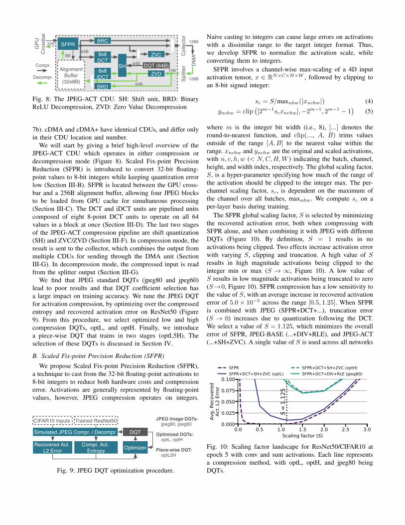
Fig. 8: The JPEG-ACT CDU. SH: Shift unit, BRD: BinaryReLU Decompression, ZVD: Zero Value Decompression

7b). cDMA and cDMA+ have identical CDUs, and differ onlyin their CDU location and number.

We will start by giving a brief high-level overview of theJPEG-ACT CDU which operates in either compression ordecompression mode (Figure 8). Scaled Fix-point PrecisionReduction (SFPR) is introduced to convert 32-bit floating-point values to 8-bit integers while keeping quantization errorlow (Section III-B). SFPR is located between the GPU cross-bar and a 256B alignment buffer, allowing four JPEG blocksto be loaded from GPU cache for simultaneous processing(Section III-C). The DCT and iDCT units are pipelined unitscomposed of eight 8-point DCT units to operate on all 64values in a block at once (Section III-D). The last two stagesof the JPEG-ACT compression pipeline are shift quantization(SH) and ZVC/ZVD (Section III-F). In compression mode, theresult is sent to the collector, which combines the output frommultiple CDUs for sending through the DMA unit (SectionIII-G). In decompression mode, the compressed input is readfrom the splitter output (Section III-G).

We find that JPEG standard DQTs (jpeg80 and jpeg60)lead to poor results and that DQT coefficient selection hasa large impact on training accuracy. We tune the JPEG DQTfor activation compression, by optimizing over the compressedentropy and recovered activation error on ResNet50 (Figure9). From this procedure, we select optimized low and highcompression DQTs, optL, and optH. Finally, we introducea piece-wise DQT that trains in two stages (optL5H). Theselection of these DQTs is discussed in Section IV.

B. Scaled Fix-point Precision Reduction (SFPR)

We propose Scaled Fix-point Precision Reduction (SFPR),a technique to cast from the 32-bit floating-point activations to8-bit integers to reduce both hardware costs and compressionerror. Activations are generally represented by floating-pointvalues, however, JPEG compression operates on integers.

JPEG Image DQTs:    jpeg80, jpeg60

Optimized DQTs:    optL, optH

Piece-wise DQT:    optL5H

Trained ResNet50CIFAR10 Inputs 

Simulated JPEG Compr. / Decompr.

Recovered Act. L2 Error

Compr. Act. Entropy

DQT

Optimizer

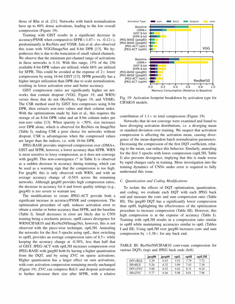
Fig. 9: JPEG DQT optimization procedure.

Naive casting to integers can cause large errors on activationswith a dissimilar range to the target integer format. Thus,we develop SFPR to normalize the activation scale, whileconverting them to integers.

SFPR involves a channel-wise max-scaling of a 4D inputactivation tensor, x ∈ RN×C×H×W , followed by clipping toan 8-bit signed integer:

sc = S/maxnhw(|xnchw|) (4)

ynchw = clip([2m−1scxnchw],−2m−1, 2m−1 − 1

)(5)

where m is the integer bit width (i.e., 8), [...] denotes theround-to-nearest function, and clip(..., A, B) trims valuesoutside of the range [A,B] to the nearest value within therange. xnchw and ynchw are the original and scaled activations,with n, c, h, w (< N,C,H,W ) indicating the batch, channel,height, and width index, respectively. The global scaling factor,S, is a hyper-parameter specifying how much of the range ofthe activation should be clipped to the integer max. The per-channel scaling factor, sc, is dependent on the maximum ofthe channel over all batches, maxnhw. We compute sc on aper-layer basis during training.

The SFPR global scaling factor, S is selected by minimizingthe recovered activation error, both when compressing withSFPR alone, and when combining it with JPEG with differentDQTs (Figure 10). By definition, S = 1 results in noactivations being clipped. Two effects increase activation errorwith varying S, clipping and truncation. A high value of Sresults in high magnitude activations being clipped to theinteger min or max (S → ∞, Figure 10). A low value ofS results in low magnitude activations being truncated to zero(S→0, Figure 10). SFPR compression has a low sensitivity tothe value of S, with an average increase in recovered activationerror of 5.0× 10−5 across the range [0.5, 1.25]. When SFPRis combined with JPEG (SFPR+DCT+...), truncation error(S → 0) increases due to quantization following the DCT.We select a value of S = 1.125, which minimizes the overallerror of SFPR, JPEG-BASE (...+DIV+RLE), and JPEG-ACT(...+SH+ZVC). A single value of S is used across all networks

0.0 0.5 1.0 1.5 2.0 2.5 3.0Scaling factor (S)

0.000

0.025

0.050

0.075

0.100

Avg.

Rec

over

edAc

t. L2

Erro

r

S=

1.12

5

SFPRSFPR+DCT+SH+ZVC (optL)

SFPR+DCT+SH+ZVC (optH)SFPR+DCT+DIV+RLE (jpeg80)

Fig. 10: Scaling factor landscape for ResNet50/CIFAR10 atepoch 5 with conv and sum activations. Each line representsa compression method, with optL, optH, and jpeg80 beingDQTs.

and layers to avoid introducing additional hyper-parametersinto training.

The channel-wise scaling factor, sc, could require the costlycalculation of the maximum of each channel in the activationmap. To avoid this, the maximum can be calculated efficientlyusing the activation statistics (mean and variance) alreadydetermined by batch normalization [24]. Alternatively, priorwork on integer quantization has shown that activation statis-tics do not vary significantly between batches [49], makinga sampling-based method a promising approach. We do notmeasure scaling factor calculation due to the many solutionswith little or no performance or hardware overhead.

SFPR, when used as a pre-stage to JPEG, has the benefit ofscale normalization. We find that without scale normalization,compression ratios vary greatly during training, and acrossdifferent networks. Compression variation across channels alsoreduces trained network accuracy. This appears to result fromdifferent input ranges to JPEG compression: activations with asmall range will be truncated, giving a high compression ratiobut also high compression error. For instance, activations witha range smaller than 1.0 result in zeros after integer casting.Scale normalization ensures that the entire 8-bit integer rangeis utilized for all activation channels with SFPR and JPEG.

The SFPR compression unit used in the JPEG-BASE andJPEG-ACT accelerator designs is divided into eight identicalSFPR Processing Elements (SPE1 to SPE8), each of whichhandle the conversion of one integer or float (Figure 11).

During the forward pass, sc is loaded when starting eachnew channel ( 1 ). Then, after the return of a cache sector(32B) through the GPU crossbar, the eight 32-bit floating-point values on this sector are split among the SPEs ( 2 ). scis multiplied with the activation using a 2-stage floating-pointmultiplier ( 3 ), and cast to an 8-bit integer ( 4 ). Casting of out-of-range values saturates, rather than truncates the resultingvalue. The results of each SPE are concatenated and saved tothe alignment buffer ( 5 ) to await JPEG compression.

During the backward pass, the inverse of the scaling factor(1/sc) is loaded ( 1 ). Inverse scaling factors can be calculatedat run time without significant overhead, as the computationcost is amortized for each channel due to the large spatialdimensions of the activations. Eight 8-bit integers (having beendecompressed using JPEG) are loaded and split among theSPEs ( 6 ) and converted back to 32-bit floating-point values.The values are multiplied by 1/sc ( 3 ) and concatenated beforebeing sent to the GPU crossbar ( 7 ).

SFPR has some similarities to DPR [13] and BFP [32].SFPR reduces hardware area versus DPR by converting to 8-bit integers instead of floats. The channel-wise scaling of BFPis similar to SFPR, however, SFPR adds scale normalization,which allows for better utilization of the integer data type.

C. Alignment Buffer

The alignment buffer is a structure designed to convertbetween the linear address space and the 8×8 blocks (H×W )required by JPEG. As the DCT is a 2D operation, it requiresthat all 64 elements in a block be available before processing.

SPE8

SPE1

×

Alig

nmen

t

GPU

32B

32B

32

8B

8B

8

321

2

7

3 4 5

6

or

Cro

ssba

r

float_to_int

int_to_float Buffe

r

Fig. 11: The SFPR unit showing 8 SFPR Processing Elements(SPEs). In forward mode (grey arrows), 8× 32-bit float valuesare multiplied by sc and cast to 8× 8-bit integers, and inbackward mode (green arrows), the integers are cast to floatsand multiplied by 1/sc.

The buffer is sized to hold enough JPEG blocks to preventduplicate cache line accesses. This requires that activationsbe padded and aligned such that the start of each cache linecoincides with a JPEG block.

The size of the alignment buffer is determined by the JPEGblock size, cache line size, activation data type, and SFPRcompression ratio. We assume an NCHW memory layout(batch, channel, height, width) for activation tensors, as ithas the highest performance for training CNNs [50], and isthe default for many frameworks [22], [23], [51]. As eachJPEG block has a height of eight elements, a single block canspan at most eight cache lines. A single 128B cache line [48]can contain values from up to four JPEG blocks with 32-bitactivations. Hence, the alignment buffer is sized to cover eightcache lines compressed to eight bits per activation, i.e. 256Bor four JPEG blocks (Figure 12). A smaller buffer would resultin duplicate cache line accesses.

The JPEG-ACT CDU requires that blocks are aligned withcache line boundaries. The access stride depends on whether

b)1x2x7x14ActivationTensora)5x1x6x6ActivationTensorW

H

N

CW

C

H

N

NCH

W

NCH

W

ReshapedAct.ReshapedAct.

1stCacheLine

1stCacheLine

WPad

NCHPad

AlignmentBuffer AlignmentBuffer

⋯

⋯

⋯ ⋯

⋯

8

32 Block1 Block2 Block3 Block4

Fig. 12: Memory layout and padding examples. Colors cor-respond to different 8 × 8 JPEG blocks and padding. Whiteoutline: First cache block boundary, Black outline: Originalactivation tensor boundary.

the activation tensor has W ≤ 32. If W ≤ 32, eight sequentialcache lines are loaded, containing exactly four JPEG blocks(Fig. 12a and 12b). If W > 32, eight cache lines with astride of W are loaded (not shown). To force alignment, wezero pad the input activations’ width up to a multiple of theJPEG block width, eight elements (W pad, Figure 12a). Ratherthan padding the height of each activation channel, we insteadpad a reshaped activation. The 4D tensors, RN×C×H×W , arereshaped to a 2D tensor, RNCH×W , and padded along thereshaped dimension (NCH pad, Figure 12b). Reshaping re-quires no data movement as only the indices are changed, andpadding in this manner requires no framework modifications.

Padding increases the memory footprint of the activationsand causes a performance overhead, however, this increaseis usually small. Padding could be performed at the hard-ware level, however, this introduces additional hardware andunaligned access overheads. It is preferable to have N ∈8, 16, 32, ... due to warp sizing on GPUs, which results inno NCH padding. Similarly, activation tensors with W ∈8, 16, 32, ... result in no W padding. Out of the datasetsand networks this work examines, only ResNet18/ImageNetand ResNet50/ImageNet [3] require padding, with a storageoverhead of 6.4% for H,W padding, and 3.0% for NCH,Wpadding on ResNet50. These overheads are low as mostactivation storage is in the widest layers of the network,making the relative size of the padded elements small.

The alignment buffer is designed with one 8B read/writeport, and one 64B read/write port. During compression, theSFPR unit may perform 8B writes, while the DCT and othercompression units perform 64B reads. Once the first JPEGblock has been loaded, the DCT stage proceeds until all 4blocks have been read (4 cycles) and the buffer is freed foruse by the next set of blocks. During decompression, roles arereversed, with 64B writes from the decompression pipeline,and 8B reads by the SFPR unit. Structuring allows us tomaintain fewer read and write ports on the buffer.

D. Discrete Cosine Transform

The DCT unit used by JPEG-BASE and JPEG-ACT isimplemented by utilizing eight 8-point 1D DCT units (Figure13). We use the well known 8-point DCT of Loeffler et al. (theLLM DCT) [52] due to its ease of pipelining, and efficient useof multipliers. The LLM implementation requires 11 multipli-cations, and 29 additions for each 8-point DCT, resulting in 88multipliers for the JPEG-ACT DCT. We implement the JPEG-ACT DCT as two passes through the 1D DCT units. Aftercomputing the DCT along the first dimension, the block istransposed and processed again for the DCT along the seconddimension. Each pass through the unit takes four cycles tocomplete. After being transformed by the 2D DCT, the blockis sent to the DIV unit for JPEG-BASE (not shown) or theSH unit for JPEG-ACT (right, Figure 13 and Section III-F).

The iDCT unit is fashioned similarly to the DCT unit. Inbrief, eight 8-point iDCT units are combined with a normal-izing shift stage. The stages are inverted relative to the DCT,i.e. multipliers become dividers, etc. This results in a similar

1D DCT 1

8B

13

6

1D DCT 8

Alig

nmen

t Buf

fer

Transpose

8B

1B

SH 64B64B

3

n Symbol Key:

>>

0

5

1234

67

0

3

4267

51

Fig. 13: The JPEG-ACT 2D DCT unit. 1D DCT is reproducedfrom the LLM fast DCT [52]. Bottom: DCT algorithm buildingblocks with cn = cos(nπ/16), sn = sin(nπ/16).

implementation with a two-pass structure and four pipelinestages.

E. DIV and RLE (JPEG-BASE)

JPEG-BASE uses a hardware implementation of the JPEGstandard quantization and coding stages. DIV quantization isa simple division by the DQT, and RLE coding combines run-length encoding and Huffman coding. We implement the DIVunit as a parallel multiplier, and use designs from OpenCoresfor RLE (encoding) [53], and RLD (decoding) [54]. Hardwareis duplicated as necessary to meet throughput requirements.

F. SH and ZVC (JPEG-ACT)

The JPEG standard was designed for software compressionof images. We developed the shift (SH) and ZVC back-end,replacing steps from the standard JPEG algorithm to reducehardware overheads and improve compression on activations.SH quantization is designed to remove the multipliers usedin the DIV stage of JPEG-BASE. ZVC coding [21] is usedbecause of our observations that activation frequency distribu-tions vary drastically from images. SH and ZVC, combinedwith SFPR and the DCT, compose the JPEG-ACT accelerator.

SH is motivated by our observations that exact quantizationis often unnecessary. By switching the division to a shiftingoperation (Figure 14), the area associated with the quantizationoperation can be reduced by 88%. This has the effect of limit-ing DQT values to powers of 2. In compression mode, 64 rightshift operations are performed in parallel. In decompressionmode, the right shifts are replaced by left shifts. SH comes atthe expense of having only eight available quantization modesfor each frequency. When performing activation compression,

DCT

iDCT

log(DQT)64x3

⋯

SH1

>>

<<

ZVC

ZVD

SH64

SH2

64B

64B64B

64B

1B

1B 1B

1B Compr.

Decompr.

Fig. 14: Shift (SH) unit showing 64 parallel units. The logDQT has 64, 3-bit outputs. Colored arrows indicate compres-sion and decompression paths.

we observe that fewer quantization modes are sufficient as theindividual effect of single frequencies is reduced (Section IV).

We use ZVC to compress the sparse result of the SH stage.After the DCT and quantization, images have most zerosat high frequency values (Figure 2). Conversely, activationsdisplay a flatter profile, with zeros randomly distributed acrossmid and high frequencies (Figure 2). Thus, ZVC has a highercompression than RLE on frequency domain activations.

The modifications of SH and ZVC decrease hardware areaby 1.5× (Section VI-F), and increase compression by up to1.4× (Section VI-C).

G. Collector and Splitter

The collector and splitter units are required to convertbetween the multiple CDU data streams and the single PCIeDMA data stream. The collector joins the variable-sizedstreams from the CDUs into a single stream. The splitter splitsthe PCIe stream by calculating and tracking the number ofbytes in each block. Both the collector and splitter connectdirectly to the PCIe DMA unit.

The scheduling policy for interleaving CDUs can have alarge impact on collector and splitter designs, hence it needsto be addressed first. The collector and splitter operate ata rate of one 8 × 8 block per cycle (Figure 15). The loador store rate to the GPU crossbar is one block per eightcycles per CDU. Hence, the entire JPEG-ACT accelerator willalways be bottlenecked by either the PCIe interconnect at lowcompression rates or the crossbar link at high compressionrates. As the CDU processing is 8× faster than the crossbarrate, we use a simple round-robin scheduling of the CDUsaccomplished with a simple mux (Figure 15), i.e. CDUs arescheduled in order with one cycle each. This also solves theissue of splitting, as streams are deterministically interleaved.

The collector unit operates during the forward pass (Figure15a). One CDU writes to the collector on each cycle with around-robin policy ( 1 ). The ZVC mask is summed to obtainthe total number of non-zero bytes in the block ( 2 ). Theprimary structure for aligning non-zero values is the 256BInput FIFO (IFIFO, 3 ). The IFIFO is designed to allow avariable-sized push operation from 0B to 72B, indexed by the

DMA

64B 8B 64B 8BCDU1 CDU4

{vals,mask}sum

⋯

72B+8

128B

DMA

CDU1

⋯

128B

256B+8

sum

pop_bytes

front_8bytes

{vals,mask}72B

8B

push_bytes

OFIFO IFIFO

7

7

b)a) CDU4

1

2

3

4 5

6

78

9

256B

Fig. 15: a) Collector and b) Splitter units for aggregating andsplitting compressed streams. Pipeline registers and controlsignals inserted as necessary.

push bytes signal. When the IFIFO fill is greater than 128B,128B is popped from the head of the IFIFO and the filledpacket is sent to the DMA unit ( 4 ). As pop operations arealways 128B, the IFIFO tail location is always at the 0th or128th byte.

The splitter unit operates during the backward pass (Figure15b). 128B packets from the DMA are pushed onto a 256BOutput FIFO (OFIFO, 5 ). Eight bytes, representing the maskof the next block to be read, are peeked from the front ofthe OFIFO ( 6 ). The mask is used to calculate the number ofbytes to pop from the OFIFO in the next cycle ( 7 and 8 ).As collection is deterministic, the distribution of blocks fromthe splitter occurs with the same round-robin policy ( 9 ).

By utilizing a collector and splitter, multiple CDUs can beused while avoiding issues with inter-cache communication.

IV. OPTIMIZING COMPRESSION

The JPEG DQTs for images (jpeg60, jpeg80, etc.) werecreated by extensively studying human perception, however,prior work indicates that CNNs have a different frequencysensitivity [55]. Optimization is performed by first definingmetrics for approximating network convergence and compres-sion, and the creation of an objective function (Figure 9). Thisresults in a significantly higher activation compression ratewith similar error relative to a JPEG DQT for images.

Network convergence is currently a poorly understood topic[56]. However, an efficient way of measuring convergence isrequired to optimize the JPEG DQT. There are no objectivefunctions to gauge the final accuracy of a network withouttraining. Therefore, we choose to maintain accuracy, ratherthan attempting to maximize accuracy.

The effect of JPEG compression on training can be under-stood by considering a single layer of a network during train-ing, with reshaped and padded activations, x ∈ RNCH×W , andweights, w. For one iteration of backprop and no compression,output activation and weight gradient are calculated as y =w ◦x, and ∇w = ∇y ◦x, respectively, where ∇y is the outputactivation gradient, and ◦ is a generic tensor dot product. Ifthe iteration is repeated using JPEG activation compression,the approximate weight gradient, ∇w∗, is calculated as:

q =(qij)=([DCT(x)ij/DQTuv]

)(6)

x∗ = iDCT((qijDQTuv

)) (7)

∇w∗ = ∇y ◦ x∗ (8)

where u, v ≡ i mod 8, j mod 8, [...] is the round-to-nearestfunction, q ∈ ZNCH×W is the quantized frequency matrix,and x∗ is the recovered activation.

The tensor dot product is a linear operation, hence the errorrelative to uncompressed can be expressed as:

∇w∗ −∇w = ∇y ◦ (x∗ − x) (9)

Identical convergence to uncompressed is achieved as theerror approaches zero. This can be accomplished by minimiz-ing the L2 activation error, using Eqn. 9 and a first orderapproximation: ‖∇w −∇w∗‖ ∝ ‖x− x∗‖.

To form the global objective function, a measure of com-pression is also required for the optimization procedure. Weuse the Shannon entropy (H , Eqn. 11) of the quantizedfrequency coefficients (q), which represents the minimum bitsrequired per activation. This, combined with the average L2error per activation (L2), form the objective function, O:

L2 = (NCHW )−1‖x− x∗‖ (10)

H =

2m−1−1∑v=−2m−1

P (q=v)log2(P (q=v)) (11)

O = (1− α)λ1H + αλ2L2 (12)

where m = 8 is the quantization bit width, P (q = v) is theprobability that q = v, determined by counting the numberof occurrences of v in q, and λ1 = 10 and λ2 = 10000are normalizing scaling factors. α is a hyper-parameter thatcontrols the rate/distortion trade-off.

We minimize O with respect to the DQT for all convolutionlayers using 240 example activations from a generator networkwith frozen weights, ResNet50/CIFAR10 trained for 5 epochs.The example activations are used to calculate L2, H , and Ofor a given DQT. SGD is used as an optimizer (lr = 2.0,p = 0) with DQT gradients calculated using forward finitedifference (difference of 5). The first of the 64 DQT parame-ters, representing the activation mean, is fixed to 8 to preventinstability in the batch normalization parameters.

We examine the rate/distortion trade-off for SFPR anddifferent JPEG DQTs to determine the efficacy of optimization(Figure 16). Optimizing the DQTs for activation compressionresults in lower error for the same compression than bothSFPR and JPEG-BASE with image DQTs, and decreasesentropy by 1 bit for the same error compared to image DQTs(optH vs. jpeg80, Figure 16).

Tuning of the DQT for the desired compression rate anderror is controlled using α, hence we select two values repre-senting low and high compression variants, optL (α = 0.025)and optH (α = 0.005), respectively. As α increases, a highercost is placed on L2 activation error, resulting in the errordecreasing from 0.10 to 0.02 with optH vs. optL (Figure 16).

optHjpeg60

SFPR (3-bit)jpeg80

optL

Fig. 16: Rate/distortion trade-off for SFPR (2-, 3-, and 4-bit),and JPEG-BASE with image DQTs (jpeg40, 60, 80, and 90)and optimized DQTs (α = 0.001, 0.005, 0.01, and 0.025).Based on ResNet50/CIFAR10 trained for 5 epochs.

10 2

10 1

100

0

2

4

10 3

10 2

10 1

100

Reco

vere

d Ac

t. Er

ror (

L 2)

0

2

4

Com

pr. A

ct. E

ntro

py (H

, bits

/act

.)

0 5 10 15 20Epoch

10 3

10 2

10 1

100

0 5 10 15 20Epoch

0

2

4

VGG

ResNet50

WRN

jpeg80 optL optH optL5H

Fig. 17: Activation error and entropy for JPEG-BASE withvarious DQTs on CIFAR10.

The values of α for optH and optL were chosen as they havea similar error to the jpeg80 and jpeg90 DQTs. This errorrange was observed to be approximately where a decrease inaccuracy begins.

We examine how compression error and entropy vary overthe course of training by evaluating each DQT on snapshots ofthe networks at different epochs (Figure 17). Activation erroris highest in the first epochs for ResNet50 and WRN (Figure17, left), which is a consequence of weight decay. However,we observe that after the first 5 epochs, compression remainsconstant. This is attributed to stable activation distributionsfrom batch normalization [24], combined with the scale nor-malization of SFPR. We observe that these trends in error andentropy continue for the remainder of training.

The first epochs of training are critically important to theconvergence of CNNs [57]. To address the critical first epochs,we propose a piece-wise approach to selecting DQTs, optL5H(Figure 17). optL5H uses the optL DQT for the first 5 epochsof training, then switches to the optH DQT for the remainderof training. This avoids high errors in the critical period.

V. METHODOLOGY

We compress the activations in each CNN according to layertype and dimensions (Table II). The use of BRC is determinedby whether a ReLU activation is followed by a conv layer,hence they are divided by subsequent layer. Sum refers todense activations produced by the addition of two activations.JPEG compression is used on conv and sum activations withsize ≥ 8, due to the 8× 8 block size of the algorithm. We donot use JPEG on the final four convolutions, or fully connectedlayers, due to their small activation size.

Datasets and networks are selected from a variety of net-work types and CNN applications. Extremely large networks,e.g. GPIPE, are not examined in this work due to highmemory requirements [9]. We evaluate JPEG-ACT using theCIFAR10 [58], ImageNet [7], and Div2k [59] datasets. Weuse six image classification CNNs: VGG-16 (VGG) [27],

TABLE I: Compression rate trade-offs. Compression ratios are bracketed, bolded values indicate highest for lossy methods.

Baseline cDMA+ GIST SFPR JPEG-BASE JPEG-ACT8-bit 8-bit jpeg80 jpeg60 optL optH optL5H

CIFAR10 % Top-1 Val. Accuracy (Compression ratio)VGG 92.1 - (1.5x) 92.7 (6.1x) 92.0 (4x) 91.4 (7.4x) 89.0 (8.3x) 92.8 (9.4x) 91.9 (12.0x) 92.4 (11.9x)ResNet50 94.5 - (1.1x) 94.4 (4.1x) 94.5 (4x) 93.6 (5.1x) 93.0 (6.0x) 94.4 (5.2x) 93.8 (7.6x) 94.4 (7.5x)ResNet101 94.7 - (1.1x) 94.4 (4.1x) 94.7 (4x) 94.0 (5.0x) 92.8 (5.8x) 94.8 (5.0x) 94.0 (7.2x) 94.5 (7.2x)WRN 95.4 - (1.6x) 95.8 (5.6x) 95.2 (4x) 92.6 (6.2x)* 91.9 (7.2x)* 95.7 (8.1x) 91.8 (11.0x)* 94.2 (10.9x)

ImageNet % Top-1 Val. Accuracy (Compression ratio)ResNet18 67.8 - (1.2x) 66.9 (3.6x) 67.9 (4x) 67.4 (5.7x) 66.6 (6.4x) 67.6 (6.1x) 66.9 (7.3x) 67.3 (7.2x)ResNet50 71.7 - (1.2x) 68.5 (3.7x) 71.4 (4x) 71.8 (5.3x) 69.8 (6.1x) 71.8 (5.1x) 28.9 (6.0x)* 71.6 (5.9x)

Div2K Val. PSNR (Compression ratio)VDSR 35.6 - (1.3x) 34.8 (4.0x) 35.5 (4x) 35.5 (5.9x) 35.3 (6.4x) 35.5 (8.2x) 35.4 (9.2x) 35.4 (9.1x)

Average % Change from Baseline (Compression ratio)All Models - 0 (1.3x) -1.07 (4.5x) -0.12 (4x) -0.87 (5.8x) -2.27 (6.6x) +0.07 (6.7x) -9.58 (8.6x) -0.38 (8.5x)

∗ run failed to converge

TABLE II: Compression selection by activation type.SD=SFPR+DCT

Method conv or ReLU ReLU pool orsum (to other) (to conv) dropout

cDMA+ None ZVCGIST DPR BRC DPR+CSRSFPR SFPRJPEG-BASE SD+DIV+RLE ∗ BRC SFPRJPEG-ACT SD+SH+ZVC ∗ BRC SFPR+ZVC

∗ for NCH,W ≥ 8, 8, otherwise SFPR.

Wide ResNet (WRN) [25], and ResNet18, 50, and 101 [3].Networks are unmodified from the original sources [22], [60].Additionally, we examine JPEG-ACT on super-resolution withVDSR [61], which is modified to use 64 × 64 random cropsand batch normalization.

We implement a functional simulation of each method inChainer [22] to examine compression and its effects on trainedneural network accuracy. The methods are implemented asCUDA code that extends the framework. We skip losslesscompression during functional simulation, instead calculatingcompression ratios offline with a batch size of 8.

Performance simulation uses GPGPU-Sim [45], [46], con-figured to simulate an NVIDIA Titan V GPU [47], and PCIe3.0 with an effective transfer rate of 12.8GB/s (Figure 7a)[19]. We model boost clocks of 1455MHz, 40 StreamingMultiprocessors, an interconnect capable of 32B/cycle bi-directional bandwidth, and 850MHz HBM. Whole-networkperformance is assessed by a microbenchmark, programmedin C++, CUDA, cuDNN, cuSPARSE, of three CNR blockssampled from each network at a batch size of 16, as fullnetworks lead to prohibitive simulation requirements. A warm-up of one ReLU is used to avoid cold start misses in the GPUcache. As source code for GIST is not publicly available wereimplemented it both for performance (CUDA and cuSparse)and functional (Chainer and CUDA) simulation. This includesthe DPR, BRC, in-place optimizations and Sparse StorageDense Compute, a Compressed Sparse Row (CSR) variant.

1.0 1.5 2.0 2.5 3.0Performance (relative to vDNN)

2.0

1.5

1.0

0.5

0.0

Avg.

Acc

urac

y/PS

NRCh

ange

(%

)

cDMA+

GIST

SFPR

jpeg80

jpeg60

optL optL5H

LosslessPrecision ReductionJPEG-BASEJPEG-ACT

Fig. 18: Percentage accuracy loss vs. relative speedup.

We implement the JPEG-ACT accelerator as RTL andsynthesize using Synopsys Design Compiler to evaluate tim-ing, area, and power requirements. Our synthesis targets theinterconnect clock frequency, and 45nm technology using theFreePDK45 design library [62]. Results are scaled to 15nm, asthe 15nm library is no longer available, and 50% wire overheadadded in a similar manner to prior works [21], [63].

VI. EVALUATION

A. Overall

Figure 18 plots percentage change in accuracy versus perfor-mance improvement. The two JPEG-ACT variants, optL andoptL5H achieve better performance gains for a given level ofaccuracy loss versus the alternatives considered in this study.

B. Compression and Accuracy

We train all networks under compression and report the bestvalidation score, i.e. the Top-1 accuracy or Peak Signal-to-Noise Ratio (PSNR), and average network compression ratio(Table I). ImageNet accuracies are lower (-4.2%) than theoriginal work [3], [64] as we use a more CPU-efficient aug-mentation procedure and report the 1-crop validation insteadof the 10-crop test accuracy.

cDMA+ is lossless, resulting in no accuracy change, how-ever, it has a low compression ratio of 1.3×. We observe ReLUand dropout compression ratios of 2.1× and 3.9×, similar to

those of Rhu et al. [21]. Networks with batch normalizationhave up to 60% dense activations, leading to the low overallcompression (Figure 19).

Training with GIST results in a significant decrease inaccuracy/PSNR when compared to SFPR (-1.07× vs. -0.12×),predominantly in ResNets and VDSR. Jain et al. also observedthis issue with VGG/ImageNet and 8-bit DPR [13]. We hy-pothesize this is due to the truncation of small valued channels.We observe that the minimum per-channel range of activationsin these networks is 0.16. With this range, 15% of the 256available 8-bit DPR values are utilized, while 66% are utilizedfor SFPR. This could be avoided at the expense of 2× lowercompression by using 16-bit GIST [13]. SFPR generally has ahigher integer utilization than DPR due to scale normalization,resulting in lower activation error and better accuracy.

GIST compression ratios are significantly higher on net-works that contain dropout (VGG, Figure 19, and WRN)versus those that do not (ResNets, Figure 19, and VDSR).The CSR method used by GIST first compresses using 8-bitDPR, then extracts non-zero values and their column index.With the optimizations made by Jain et al., this requires thestorage of an 8-bit DPR value and an 8-bit column index pernon-zero value [13]. When sparsity is <50%, size increasesover DPR alone, which is observed for ResNets on ImageNet(Table I), making CSR a poor choice for networks withoutdropout. CSR is advantageous when the compressed valuesare larger than the indices, i.e. with 16-bit DPR.

JPEG-BASE provides improved compression over cDMA+,GIST and SFPR, however, a lower accuracy than SFPR. WRNis most sensitive to lossy compression, as it does not convergewith jpeg80. This non-convergence (* in Table I) is observedas a sudden decrease in accuracy during training, which canbe used as a warning sign that the compression is too high.For jpeg80, this is only observed with WRN, and with anaverage accuracy change of -0.54% across the remainingnetworks. Although jpeg60 provides high compression ratios,the decrease in accuracy for it and lower quality settings (e.g.,jpeg40) is too severe to warrant use.

The modifications to create JPEG-ACT provide both asignificant increase in accuracy/PSNR and compression. Theoptimization procedure of optL reduces activation error toobtain a similar or better accuracy than SFPR, and the baseline(Table I). Small decreases in error are likely due to CNNtraining being a stochastic process. optH causes divergence forWRN/CIFAR10 and ResNet50/ImageNet, however, this is notobserved with the piece-wise technique, optL5H. Annealingthe networks for the first 5 epochs using optL, then switchingto optH, provides an average compression ratio of 8.5× whilekeeping the accuracy change at -0.38%, less than half thatof GIST. JPEG-ACT with optL5H increases compression overJPEG-BASE with jpeg80 both by having a higher quantizationfrom the DQT, and by using ZVC on sparse activations.Higher quantization has a larger effect on sum activations,with conv activation compression remaining mostly unchanged(Figure 19). ZVC can compress ReLU and dropout activationsto further decrease their size after SFPR, with a relative

BaselinecDMA+

GIST 8-bitSFPR 8-bit

JPEG-BASE (jpeg80)JPEG-BASE (jpeg60)

JPEG-ACT (optL)JPEG-ACT (optH)

0.0 0.2 0.4 0.6 0.8 1.0Memory Consumption (Relative to Baseline)

BaselinecDMA+

GIST 8-bitSFPR 8-bit

JPEG-BASE (jpeg80)JPEG-BASE (jpeg60)

JPEG-ACT (optL)JPEG-ACT (optH)

VGG

ResNet50

Activation Type: sum ReLU dropout conv

Fig. 19: Activation footprint breakdown by activation type forCIFAR10 models.

contribution of 1.1× to total compression (Figure 19).Networks that do not converge were examined and found to

have diverging activation distributions, i.e. a diverging meanor standard deviation over training. We suspect that activationcompression is affecting the activation mean, causing diver-gence of the mean-dependent batch normalization parameters.Decreasing the compression of the first DQT coefficient, relat-ing to the mean, can reduce this behavior. Similarly, annealingfor the first 5 epochs with lower compression (optL5H, TableI) also prevents divergence, implying that this is made worseby rapid changes early in training. More investigation into thetraining dynamics of CNNs under error is required to fullyunderstand this issue.

C. Quantization and Coding Modifications

To isolate the effects of DQT optimization, quantization,and coding, we evaluate each DQT with each JPEG backend and measure the conv and sum compression ratio (TableIII). The jpeg80 DQT has a significantly lower compressionthan optH, highlighting the effectiveness of the optimizationprocedure to increase compression (Table III). However, thishigh compression is at the expense of accuracy (Table I).Training with optL5H results in a compression ratio similarto optH while maintaining accuracies similar to optL (TablesI and III). Using optL5H over jpeg80 increases conv and sumcompression by >1.38× for any back end.

TABLE III: ResNet50/CIFAR10 conv+sum compression forvarious DQTs (top) and JPEG back ends (left)

jpeg80 jpeg60 optL optH optL5HDIV+RLE 5.29 6.43 3.52 7.79 7.72SH+RLE 5.26 6.32 3.99 7.43 7.38DIV+ZVC 5.80 6.52 4.62 8.31 8.24SH+ZVC 5.77 6.46 5.08 8.01 7.96

VGGCIFAR10

ResNet50CIFAR10

ResNet101CIFAR10

WRNCIFAR10

ResNet18ImageNet

ResNet50ImageNet

VDSRDIV2K

Average0

1

2

3

4Pe

rform

ance

(vDN

N=1) 4.5 vDNN

cDMA+GIST 8-bit

SFPR 8-bitJPEG-BASE (jpeg80)JPEG-BASE (jpeg60)JPEG-ACT (optL)JPEG-ACT (optH)JPEG-ACT (optL5H)

Infinite Memory

Fig. 20: Relative performance to vDNN.

The use of ZVC over RLE increases the compressionratio by 1.12×. In JPEG-BASE, RLE is used because high-frequency information has a low magnitude, leading to mosthigh-frequency values being zero after quantization. CNNactivations, however, have much larger high-frequency modes,which are quantized to non-zero values. RLE performs poorlywith randomly distributed zeros in contrast to ZVC. Addition-ally, the optimized DQTs have a flatter quantization profilewhen compared to image DQTs. This low-frequency quanti-zation further randomizes zeros and is especially apparent inthe improvement of optL when using ZVC (1.3×).

D. Performance

Performance measurement is accomplished through micro-benchmarking using CNR blocks with an optional dropout orpooling layer. Due to simulation time and memory constraints,we simulate three layers of each network (the first, middle,and last), and use a batch size of 16. The algorithms usedare WINOGRAD, and WINOGRAD NONFUSED for 3 × 3convolutions, and IMPLICIT GEMM and ALGO 0 for 1× 1convolutions. This is representative of software frameworkssuch as Chainer and Pytorch [46].

GIST performance is strongly influenced by networkstructure (Figure 20). Poor performance on ResNet50 andResNet101 can be attributed to the presence of bottlenecklayers [3], which involve 1 × 1 convolution to decrease thenumber of channels. Bottlenecks involve up to 2048 channels,creating large activations with 9× fewer FLOPs than a sim-ilarly sized 3 × 3 kernel. The non-zero scan in the cuSparsedense2CSR conversion takes longer than a 1×1 kernel, in thiscase, creating a large performance overhead.

By comparison, SFPR and JPEG-ACT display performancethat is not network dependent. The SFPR-only design pro-vides 1.35× performance over GIST despite having a lowercompression, primarily because CSR is slower than SFPR.The PCIe bandwidth limitations are nearly eliminated byJPEG-ACT with optL5H, giving a performance increase overGIST of 1.59× and overhead of 1.13×. More consistentperformance is obtained by shifting the bottleneck to effectiveoffload rate instead of compression throughput. Compressionincreases that result from modifying JPEG for CNNs, improveperformance by 1.12× while decreasing the error changefrom baseline by 2.3× (JPEG-ACT optL5H vs. JPEG-BASEjpeg80). We observe that the remaining overheads of JPEG-

1x 2x 4x 8x 12xCompression ratio

0.0

0.5

1.0

Rela

tive

Runt

ime

DMA-side # CDUs:Cache- + DMA-side # CDUs:

148+4

2 4 8

Fig. 21: Performance when changing the number of CDUs onResNet50/CIFAR10 with a fixed compression ratio. Cache- +DMA-side refers to Cache-size SFPR CDUs, and DMA-sideDCT+SH+ZVC CDUs.

ACT are caused by congestion on the GPU interconnect fromthe increase in DMA traffic. Despite this, JPEG-ACT obtains2.61× performance versus vDNN.

VDSR has 1.4× to 2.3× worse offload performance than theother networks (Figure 20). VDSR has no dropout, pooling,or bottleneck layers, however, the most important differenceis that all activations have few channels and a large spatialdimension. We have observed that cuDNN launches a differentset of compute kernels for VDSR, and hypothesize that themethod used has a lower compute density, resulting in pooroffload performance.

E. CDU Count and Location

The effective offload rate available to JPEG-ACT is highlydependent on the location and configuration of the CDUs inthe GPU memory system. Most importantly, the number ofCDUs affects the available bandwidth into the GPU (Figure21). With DMA-side compression, there is little increase inperformance over 1 CDU at 2× and 4× compression as theoffload is bottlenecked by the PCIe offload rate. At 8× and12× compression, however, the bottleneck is removed, andperformance increases as CDUs are added. Performance for12× compression increases by 1.08× when moving from 2to 4 CDUs, but by less than 0.5% when moving from 4 to 8CDUs. At this compression and number of CDUs, the memorypartitions become the bottleneck, preventing further increases.

We also examine the impact of moving the SFPR portion ofthe CDU to the L2 cache in a combined Cache- and DMA-sidecompression (Figure 21). In this configuration in the forwardpass, values from the cache are immediately compressed by

TABLE IV: JPEG-ACT synthesis by component

Component Area (um2) Power (mW)SFPR 44924 34.3DCT + iDCT 229118 273.4Quantize (DIV) 12507 14.4Quantize (SH) 1593 2.5Coding (RLE + RLD) 125890 176.0Coding (ZVC + ZVD) 21519 17.1Collector + Splitter 173445 170.3Crossbar (+3 ports) 2253427 1668.0

TABLE V: Designs comparison with buffers and 4 CDUs.Crossbar excluded.

cDMA+ SFPR JPEG-BASE JPEG-ACT(jpeg80) (optL5H)

Power (W) 0.26 0.35 1.82 1.36Area (mm2) 0.35 0.31 2.16 1.48Compression 1.3x 4.0x 5.8x 8.5xOffload (GB/s) 15.6 48.0 69.6 108.8

SFPR, sent over the GPU interconnect, and compressed againby JPEG before the DMA unit. The minimum compressionrate is 4× due to the mandatory use of SFPR. As thereis one SFPR unit per memory partition, there are 48 SFPRCDUs and 4 JPEG CDUs. This configuration has a high areaoverhead due to duplication of the SFPR units and results in aperformance increase of 1% over a 4 CDU DMA-side design.

F. Synthesis

Power and area results for the individual JPEG-ACT compo-nents (Table IV), indicate that the DCT is the most expensivecomponent of JPEG-ACT, followed by the required buffers.The overall area and power for each design are visible in TableV. When compared to cDMA+, JPEG-ACT provides a signif-icant increase in effective PCIe bandwidth while maintainingan area and power <1% of an NVIDIA Titan V GPU. Thisis even smaller relative to larger data center GPUs [65]. Themodifications to the JPEG-ACT back end for CNNs reduceoverall area and power by 1.3× and 1.5× , respectively, whileincreasing available PCIe offload bandwidth.

VII. RELATED WORK

We compare favorably against the primary works examiningactivation storage during training, i.e. vDNN [19], cDMA[21], and GIST [13]. However, there are many proposalsfor compressing pre-trained neural networks to reduce costsat inference , which, unlike JPEG-ACT, do not decreaseactivation storage during training [33]–[37], [66]–[70]. Thesemethods include frequency transforms [68], [69] and precisionreduction [33]–[37], [70]. Training networks with a reducedprecision (e.g. 1, 3, or 8 bits), while effective, requiresmodification of the CNN framework, network architecture, andtraining schedule [33]–[37], which is not necessary with JPEG-ACT. Other works have examined reduced precision gradientstorage for multi-GPU training, which does not decrease localmemory consumption [71].

Stored activations can be removed entirely, either throughremoving gradients [72] or by using reversible networks [12].These methods involve a much higher computational load thanmore conventional compression methods, as gradients [72]or convolutional activations [12] need to be regenerated. Incontrast to JPEG-ACT, this restricts the available layer typesof the network.

VIII. CONCLUSION

We have presented JPEG-ACT, a novel offload acceleratorfor CNN activation compression, and its fixed-point com-pression mechanism Scaled Fix-point Precision Reduction(SFPR). Our results demonstrate JPEG-ACT can be effectivelyused on a wide variety of datasets and benchmarks, andprovides significantly higher compression ratios than the state-of-the-art. JPEG can be further tuned for CNNs, providing a1.5× improvement in compression, while increasing trainedaccuracy. Given hardware support, JPEG-ACT can be incor-porated simply with any CNN architecture and framework

REFERENCES

[1] A. Krizhevsky, “Convolutional Neural Networks for Object Classifi-cation in CUDA,” University of Toronto, EECE1742S: ProgrammingMassively Parallel Multiprocessors Using CUDA, April 2009.

[2] A. Krizhevsky, I. Sutskever, and G. E. Hinton, “ImageNet Classificationwith Deep Convolutional Neural Networks,” in Proc. Int. Conf. onNeural Information Processing Systems (NeurIPS), 2012.

[3] K. He, X. Zhang, S. Ren, and J. Sun, “Deep Residual Learning forImage Recognition,” in Proc. IEEE/CVF Conf. on Computer Vision andPattern Recognition (CVPR), 2016, pp. 770–778.

[4] T.-Y. Lin, P. Dollr, R. Girshick, K. He, B. Hariharan, and S. Belongie,“Feature Pyramid Networks for Object Detection,” arXiv:1612.03144[cs], 2016.

[5] J. Yao, S. Fidler, and R. Urtasun, “Describing the scene as a whole:Joint object detection, scene classification and semantic segmentation,”in CVPR, 2012, pp. 702–709.

[6] D. E. Rumelhart, G. E. Hinton, and R. J. Williams, “Learning internalrepresentations by error-propagation,” in Parallel Distributed Process-ing: Explorations in the Microstructure of Cognition, 1986.

[7] J. Deng, W. Dong, R. Socher, L.-J. Li, K. Li, and L. Fei-Fei, “ImageNet:A Large-Scale Hierarchical Image Database,” in CVPR, 2009.

[8] E. Real, A. Aggarwal, Y. Huang, and Q. V. Le, “Regularized Evolutionfor Image Classifier Architecture Search,” in Proc. AAAI Conf. onArtificial Intelligence, 2019, pp. 4780–4789.

[9] Y. Huang et al., “GPipe: Efficient Training of Giant Neural Networksusing Pipeline Parallelism,” in NeurIPS, 2019, pp. 103–112.

[10] M. Tan and Q. Le, “EfficientNet: Rethinking model scaling for con-volutional neural networks,” in Proc. Int. Conf. on Machine Learning(ICML), 2019, pp. 6105–6114.

[11] T. Chen, B. Xu, C. Zhang, and C. Guestrin, “Training Deep Nets withSublinear Memory Cost,” arXiv:1604.06174v2 [cs], 2016.

[12] A. N. Gomez, M. Ren, R. Urtasun, and R. B. Grosse, “The ReversibleResidual Network: Backpropagation Without Storing Activations,” inNeurIPS, 2017, pp. 2214–2224.

[13] A. Jain, A. Phanishayee, J. Mars, L. Tang, and G. Pekhimenko, “Gist:Efficient Data Encoding for Deep Neural Network Training,” in Proc.ACM/IEEE Int. Symp. on Computer Architecture (ISCA), 2018, pp. 776–789.

[14] G. Pekhimenko, V. Seshadri, O. Mutlu, P. B. Gibbons, M. A. Kozuch,and T. C. Mowry, “Base-delta-immediate compression: practical datacompression for on-chip caches,” in Proc. ACM Int. Conf. on ParallelArchitectures and Compilation Techniques (PACT), 2012, p. 377.

[15] M. Ekman and P. Stenstrom, “A robust main-memory compressionscheme,” in ISCA, 2005, pp. 74–85.

[16] E. Hallnor and S. Reinhardt, “A Unified Compressed Memory Hierar-chy,” in HPCA, 2005, pp. 201–212.

[17] R. B. Tremaine, P. A. Franaszek, J. T. Robinson, C. O. Schulz, T. B.Smith, M. E. Wazlowski, and P. M. Bland, “IBM Memory Expan-sion Technology (MXT),” IBM Journal of Research and Development,vol. 45, no. 2, pp. 271–285, 2001.

[18] B. Abali, H. Franke, Xiaowei Shen, D. Poff, and T. Smith, “Performanceof hardware compressed main memory,” in HPCA, 2001, pp. 73–81.

[19] M. Rhu, N. Gimelshein, J. Clemons, A. Zulfiqar, and S. W. Keckler,“vDNN: Virtualized deep neural networks for scalable, memory-efficientneural network design,” in MICRO, 2016, pp. 1–13.

[20] Y. Kwon and M. Rhu, “Beyond the memory wall: a case for memory-centric HPC system for deep learning,” in MICRO, 2018, pp. 148–161.

[21] M. Rhu, M. O’Connor, N. Chatterjee, J. Pool, Y. Kwon, and S. W.Keckler, “Compressing DMA Engine: Leveraging Activation Sparsityfor Training Deep Neural Networks,” in Proc. IEEE Int. Symp. on High-Performance Computer Architecture (HPCA), 2018, pp. 78–91.

[22] S. Tokui et al., “Chainer: A deep learning framework for acceleratingthe research cycle,” in Proc. ACM/SIGKDD Int. Conv. on KnowledgeDiscovery & Data Mining. ACM, 2019, pp. 2002–2011.

[23] A. Paszke et al., “Automatic differentiation in PyTorch,” in NeurIPSAutodiff Workshop, 2017.

[24] S. Ioffe and C. Szegedy, “Batch Normalization: Accelerating DeepNetwork Training by Reducing Internal Covariate Shift,” in ICML, 2015.

[25] S. Zagoruyko and N. Komodakis, “Wide Residual Networks,”arXiv:1605.07146 [cs], 2016.

[26] A. G. Howard, M. Zhu, B. Chen, D. Kalenichenko, W. Wang, T. Weyand,M. Andreetto, and H. Adam, “MobileNets: Efficient ConvolutionalNeural Networks for Mobile Vision Applications,” arXiv:1704.04861v1[cs.CV], 2017.

[27] K. Simonyan and A. Zisserman, “Very Deep Convolutional Networksfor Large-Scale Image Recognition,” arXiv:1409.1556 [cs], 2014.

[28] Y. Chen et al., “DaDianNao: A Machine-Learning Supercomputer,” inMICRO, 2014, pp. 609–622.

[29] Y.-H. Chen, T.-J. Yang, J. Emer, and V. Sze, “Eyeriss v2: A FlexibleAccelerator for Emerging Deep Neural Networks on Mobile Devices,”arXiv:1807.07928 [cs], 2018.

[30] A. Delmas Lascorz et al., “Bit-Tactical: A Software/Hardware Approachto Exploiting Value and Bit Sparsity in Neural Networks,” in Proc. ACMInt. Conf. on Architectural Support for Programming Languages andOperating Systems (ASPLOS), 2019, pp. 749–763.

[31] J. Albericio, P. Judd, T. Hetherington, T. Aamodt, N. E. Jerger, andA. Moshovos, “Cnvlutin: Ineffectual-Neuron-Free Deep Neural NetworkComputing,” in ISCA, 2016, pp. 1–13.

[32] M. Courbariaux, Y. Bengio, and J. David, “Training deep neural net-works with low precision multiplications,” arXiv:1412.7024 [cs], 2014.

[33] ——, “BinaryConnect: Training Deep Neural Networks with binaryweights during propagations,” in NeurIPS, 2015, pp. 3123–3131.

[34] S. Wu, G. Li, F. Chen, and L. Shi, “Training and Inference with Integersin Deep Neural Networks,” in ICLR, 2018.

[35] I. Hubara, M. Courbariaux, D. Soudry, R. El-Yaniv, and Y. Bengio,“Binarized Neural Networks,” in NeurIPS, 2016, pp. 4107–4115.

[36] M. Rastegari, V. Ordonez, J. Redmon, and A. Farhadi, “XNOR-Net:ImageNet Classification Using Binary Convolutional Neural Networks,”in Proc. European Conf. on Computer Vision, 2016, pp. 525–542.

[37] F. Li, B. Zhang, and B. Liu, “Ternary Weight Networks,”arXiv:1605.04711 [cs], 2016.

[38] D. Williamson, “Dynamically scaled fixed point arithmetic,” in Proc.IEEE Pacific Rim Conf. on Communications, Computers, and SignalProcessing, 1991, pp. 315–318.

[39] A. Robinson and C. Cherry, “Results of a prototype television bandwidthcompression scheme,” Proc. IEEE, vol. 55, no. 3, pp. 356–364, 1967.

[40] Y. Zhang, J. Yang, and R. Gupta, “Frequent value locality and value-centric data cache design,” in ASPLOS, 2000, pp. 150–159.

[41] G. K. Wallace, “The JPEG still picture compression standard,” IEEETransactions on Consumer Electronics, vol. 38, no. 1, 1992.

[42] M. Brenon and C. Deltheil, “A lightweight and portable JPEG encoderwritten in C.: Moodstocks/jpec,” 2018, original-date: 2012-01-06.[Online]. Available: https://github.com/Moodstocks/jpec

[43] M. Rabbani, “JPEG2000: Image Compression Fundamentals, Standardsand Practice,” Journal of Electronic Imaging, vol. 11, no. 2, 2002.

[44] J. Aczl and Z. Darczy, On Measures of Information and Their Charac-terizations. Academic Press, 1975.

[45] A. Bakhoda, G. L. Yuan, W. W. L. Fung, H. Wong, and T. M. Aamodt,“Analyzing CUDA workloads using a detailed GPU simulator,” in Proc.

IEEE Int. Symp. on Performance Analysis of Systems and Software(ISPASS), 2009, pp. 163–174.

[46] J. Lew et al., “Analyzing Machine Learning Workloads Using a DetailedGPU Simulator,” in ISPASS, 2019, pp. 151–152.

[47] M. Khairy, J. Akshay, T. Aamodt, and T. G. Rogers, “Exploring ModernGPU Memory System Design Challenges through Accurate Modeling,”arXiv:1810.07269 [cs], 2018.

[48] Z. Jia, M. Maggioni, B. Staiger, and D. P. Scarpazza, “Dissect-ing the NVIDIA Volta GPU Architecture via Microbenchmarking,”arXiv:1804.06826 [cs], 2018.

[49] B. Jacob, S. Kligys, B. Chen, M. Zhu, M. Tang, A. Howard, H. Adam,and D. Kalenichenko, “Quantization and training of neural networks forefficient integer-arithmetic-only inference,” in CVPR, 2018.

[50] H. Kim, H. Nam, W. Jung, and J. Lee, “Performance analysis of CNNframeworks for GPUs,” in ISPASS, 2017, pp. 55–64.

[51] M. Abadi et al., “Tensorflow: A system for large-scale machinelearning,” in Proc. USENIX Symp. on Operating Systems Design andImplementation (OSDI), 2016, pp. 265–283.

[52] C. Loeffler, A. Ligtenberg, and G. Moschytz, “Practical fast 1-D DCTalgorithms with 11 multiplications,” in Proc. Int. Conf. on Acoustics,Speech, and Signal Processing, 1989, pp. 988–991 vol.2, iSSN: 1520-6149.

[53] D. Lundgren, “JPEG Encoder Verilog,” 2009. [Online]. Available:https://opencores.org/projects/jpegencode

[54] H. Ishihara, “JPEG Decoder,” 2006. [Online]. Available: https://opencores.org/projects/djpeg

[55] I. J. Goodfellow, J. Shlens, and C. Szegedy, “Explaining and HarnessingAdversarial Examples,” arXiv:1412.6572 [cs, stat], 2015.

[56] H. Li, Z. Xu, G. Taylor, C. Studer, and T. Goldstein, “Visualizing theLoss Landscape of Neural Nets,” in NeurIPS, 2018, pp. 6389–6399.

[57] E. Hoffer, I. Hubara, and D. Soudry, “Train longer, generalize better:closing the generalization gap in large batch training of neural networks,”arXiv:1705.08741 [cs, stat], 2017.

[58] A. Krizhevsky, “Learning multiple layers of features from tiny images,”Master’s thesis, Univ. of Toronto, 2009.

[59] E. Agustsson and R. Timofte, “Ntire 2017 challenge on single imagesuper-resolution: Dataset and study,” in CVPR Workshops, 2017.

[60] S. Saito, “chainer-cifar10: Various CNN models including for CIFAR10with Chainer,” 2018, original-date: 2015-06-09T14:39:43Z. [Online].Available: https://github.com/mitmul/chainer-cifar10

[61] J. Kim, J. Kwon Lee, and K. Mu Lee, “Accurate Image Super-ResolutionUsing Very Deep Convolutional Networks,” in CVPR, 2016, pp. 1646–1654.

[62] J. E. Stine et al., “Freepdk: An open-source variation-aware design kit,”in Proc. IEEE Int. Conf. on Microelectronic Systems Education (MSE),2007, pp. 173–174.

[63] M. Martins, J. M. Matos, R. P. Ribas, A. Reis, G. Schlinker, L. Rech,and J. Michelsen, “Open Cell Library in 15nm FreePDK Technology,”in Proc. Int. Symp. on Physical Design, 2015, pp. 171–178.

[64] P. Mattson et al., “Mlperf training benchmark,” 2019.[65] NVIDIA Corporation, “Tesla V100 Datacenter GPU: NVIDIA,”

2018. [Online]. Available: https://www.nvidia.com/en-us/data-center/tesla-v100

[66] S. Han, H. Mao, and W. J. Dally, “Deep Compression: CompressingDeep Neural Networks with Pruning, Trained Quantization and HuffmanCoding,” arXiv:1510.00149v5 [cs.CV], 2016.

[67] F. N. Iandola, S. Han, M. W. Moskewicz, K. Ashraf, W. J. Dally,and K. Keutzer, “SqueezeNet: AlexNet-level accuracy with 50x fewerparameters and <0.5mb model size,” arXiv:1602.07360 [cs], 2016.

[68] Y. Wang, C. Xu, S. You, D. Tao, and C. Xu, “CNNpack: PackingConvolutional Neural Networks in the Frequency Domain,” in NeurIPS,2016, pp. 253–261.

[69] C. Ding et al., “CirCNN: Accelerating and Compressing Deep NeuralNetworks Using Block-circulant Weight Matrices,” in MICRO, 2017, pp.395–408.

[70] E. Park, J. Ahn, and S. Yoo, “Weighted Entropy Based Quantization forDeep Neural Networks,” in CVPR, 2017, pp. 7197–7205.

[71] Y. Lin, S. Han, H. Mao, Y. Wang, and W. J. Dally, “Deep GradientCompression: Reducing the Communication Bandwidth for DistributedTraining,” arXiv:1712.01887 [cs, stat], 2017.

[72] M. Jaderberg, W. M. Czarnecki, S. Osindero, O. Vinyals, A. Graves,D. Silver, and K. Kavukcuoglu, “Decoupled Neural Interfaces usingSynthetic Gradients,” ArXiv e-prints, 2016.