JOURNAL OF SELECTED TOPICS IN SIGNAL PROCESSING, VOL. 6, NO. 1, JANUARY 2013 1

Space-time signal processing for distributed patterndetection in sensor networks

*Randy Paffenroth, Philip du Toit, Ryan Nong, Louis Scharf, Life Fellow, IEEE,Anura Jayasumana, Senior Member, IEEE, and Vidarshana Bandara

Abstract—A theory and algorithm for detecting and classi-fying weak, distributed patterns in network data is presented.The patterns we consider are anomalous temporal correlationsbetween signals recorded at sensor nodes in a network. We userobust matrix completion and second order analysis to detectdistributed patterns that are not discernible at the level ofindividual sensors. When viewed independently, the data at eachnode cannot provide a definitive determination of the underlyingpattern, but when fused with data from across the networkthe relevant patterns emerge. We are specifically interestedin detecting weak patterns in computer networks where thenodes (terminals, routers, servers, etc.) are sensors that providemeasurements (of packet rates, user activity, central processingunit usage, etc.). The approach is applicable to many other typesof sensor networks including wireless networks, mobile sensornetworks, and social networks where correlated phenomena areof interest.

Index Terms—Pattern detection, matrix completion, robustprincipal component analysis, anomaly detection, `1 methods.

I. INTRODUCTION

We present an approach for detecting sparsely correlatedphenomena in sensor networks. The patterns of interest areweak and distributed across the network so that they areinherently undetectable at the level of an individual node. Onlywhen data is aggregated across the network both spatiallyand temporally, and appropriately analyzed are the relevantpatterns revealed — an approach we refer to as space-timesignal processing.

During a distributed attack, the time series at any givenlink or node may not appear suspicious or unusual, but whenexamined in the context of multiple correlated links withrespect to prevailing network conditions, the distributed patternappears as a discernible correlated anomaly.

Our work leverages recent progress in compressed sens-ing [1], matrix completion [2], robust principal componentanalysis [3]–[5], and simple model discovery [6] to provide amathematical foundation and computational framework for anunsupervised learning algorithm that detects weak, distributedanomalies in sensor data. This is in contrast to supervised

R. Paffenroth (corresponding author at randy.paffenroth@numerica.us),P. du Toit, and Ryan Nong are with Numerica Corporation, 4850 Hahns Peak,Suite 200, Loveland, CO 80538, USA.

L. Scharf is with the Department of Mathematics at Colorado StateUniversity, Fort Collins, CO 80523, USA.

A. Jayasumana, and V. Bandara are with the Department of Computer andElectrical Engineering at Colorado State University, Fort Collins, CO 80523,USA.

Manuscript received August 7, 2012.

learning algorithms in data mining [7]–[9] and machine learn-ing [10]–[13] that typically require large amounts of labeledtraining data, predefined models, or expert knowledge.

Our definition of “pattern” is based upon the principlesof low-rank and sparsity. Data collected from a network isflagged as patterned if a sparse subset of nodes exhibitscorrelations that cannot be explained by the low-rank back-ground correlation that broadly affects the entire network.These correlated anomalies can range from short duration highintensity effects, to longer duration lower intensity effects.As demonstrated by our results on measured data from theAbilene Internet2 network, both types of phenomena appearin real data and can be detected by our second-order analysis.

We must clarify that detection of distributed patterns doesnot in and of itself constitute detection of attacks — anomaliesdo not necessarily imply malicious behavior. By design, ourgoal is not to assign value judgements to network behavior inorder to determine whether actors are bad, nor do we providea long list of semantic rules for identifying malicious intent.Rather, we sift through large amounts of raw data and pinpointsensors displaying unusual patterns of behavior that are out ofstep with the norm.

Automated real-time detection of abnormally correlatedconditions can in turn trigger efforts to mitigate attacks, andcan invoke network management responses to better diagnosenetwork problems and meet quality of service targets. Fastidentification of geographically distributed sensors related tothe same abnormal condition can lead to more focused andeffective counter-measures.

The proposed algorithm helps to mitigate false alarms byonly flagging patterns that are anomalously correlated acrossmultiple sensors so that greater consensus is required before aflag is raised. Our approach is similar in spirit to recent work incollaborative anomaly detection [14], but our methods proceedfrom a more mathematical, rather than empirical, perspective.

The computational core of the analysis is phrased as aconvex optimization problem that can be solved efficiently onlarge datasets. The algorithm can detect anomalies even whenthe data of interest is distributed across multiple databasesand is too large to aggregate at a centralized location forprocessing. Recent techniques in matrix completion [2]–[4],[15] allow for efficient analysis of large correlation matricesthat, due to constraints imposed by network topologies, maybe only partially observed.

We anticipate that the mathematical framework and algo-rithms developed herein will be applicable to very generalclasses of sensor networks including networked infrastruc-

2 JOURNAL OF SELECTED TOPICS IN SIGNAL PROCESSING, VOL. 6, NO. 1, JANUARY 2013

tures, electrical grids, computer networks, aerial surveillancenetworks, disease outbreaks, and social networks. We focus oncomputer networks as a motivating application area; however,we do not make any assumptions or heuristic arguments thatare specific to computer networks. The results and expositionin this paper extend the results reported in two conferencepapers presented at the 2012 SPIE meeting [16], [17].

Our contributions include a new formulation of RobustPrincipal Component Analysis that combines robustness tonoise with partial observations. Our methods uses point-wiseerror constraints that allow entries of the matrix to havedifferent noise properties, as opposed to the standard Frobeniusnorm approach that applies a single global noise constraint. Wepresent a stability theorem and an algorithm for addressingnoisy problems with partial observations based upon a novelequivalent problem formulation that allows solution of theoptimization using a standard Alternating Direction Methodof Multipliers. We apply the method to second-order matricesto detect sparsely correlated phenomena in measured data fromthe Abilene Internet2 network.

The remainder of the paper is organized as follows: Sec-tion II elaborates the underlying theory, assumptions, andimplementation of the algorithm. Results and a discussion onthe outcomes are presented in Section III. Concluding remarksalong with future directions are highlighted in Section IV. Theappendix provides proof of Theorem 2.1.

II. METHODS, ASSUMPTIONS, AND PROCEDURES

A. Theoretical Background for Matrix Decomposition

We use several matrix norms in our analysis. Let ‖·‖∗ denotethe nuclear norm: if σ1, · · · , σm are the singular values ofmatrix A, then

‖A‖∗ :=

m∑i=1

σi .

The two-norm, denoted ‖ · ‖, returns the largest singular valueof the operator A:

‖A‖ := maxiσi .

We also refer to the following elementwise norms: the Frobe-nius norm,

‖A‖F :=

√∑ij

A2ij ,

the one-norm,

‖A‖1 :=∑ij

|Aij | ,

and the inifinity-norm,

‖A‖∞ := maxij|Aij | .

Let 〈·, ·〉 denote the matrix inner-product,

〈A,B〉 := trace(ATB),

so that ‖A‖2F = 〈A,A〉. We introduce PΩ(A), the projectionof the matrix A onto the set of entries indexed by the indicesin the set Ω, as follows:

[PΩ(A)]ij :=

Aij ij ∈ Ω0 otherwise . (1)

Also define the shrinkage operator Sε : R→ R as:

Sε(x) := sign(x) max(|x| − ε, 0). (2)

This shrinkage operator can be extended to matrix shrinkageby applying the scalar shrinkage operator to each element ofthe matrix using a matrix-valued ε. Also, we define the rankshrinkage operator Dτ : Rm×n → Rm×n as the shrinkageoperator on singular values:

Dτ (X) := USτ (Σ)V ∗,

where X = UΣV ∗ is any singular value decomposition of X .We use the “(·)0” subscript to denote truth, as in the true L0

and S0, and L and S to denote quantities we recover from thegiven data using our algorithm.

In the prototypical Principal Component Pursuit (PCP)problem, we are given a matrix M that is formed by

M = L0 + S0,

where L0 is low-rank, S0 is sparse, and we are asked torecover L0 and S0. As noted in [4], the matrix decompositionproblem may appear somewhat daunting. Given a full-rankmatrix M , we must tease out the underlying low rank matrixL0, and identify the sparse anomalies introduced by S0,without knowing a priori the true rank of L0, and withoutknowing the number or locations of the nonzero entries inS0. Furthermore, the magnitude of the few nonzero entries inS0 may be of arbitrarily large size. These difficulties may befurther compounded by failure to observe a subset of entries inM , and by noise that adds small errors to each of the remainingentries.

Remarkably, Theorem 1.2 in [4] provides the followingguarantee for matrix decomposition and recovery. IfM = L0 + S0, and we are given only PΩ(M), and ifcertain identifiability, rank, and sparsity conditions on L0, S0,and Ω are met; then, with high probability the convex program:

[Principal Component Pursuit]

minL,S‖L‖∗ + λ‖S‖1 (3)

subject to PΩ(M) = PΩ(L+ S),

with λ =√

m|Ω| exactly recovers the low rank matrix L0,

as well as the entries of the sparse matrix S′0 := PΩ(S0).1

Thus, the use of the nuclear and `1 norms allows for thedecomposition of a patterned correlation matrix into low-rankand sparse constituents using a convex program even whenthe correlation matrix is only partially observed. The problem

1Technical details of the theorem place conditions on the rank of L0, thesparsity of S0, and the size of the observed set Ω, and also requires that thecolumns of L0 are incoherent — meaning far from the standard basis, andthat the nonzero entries in S0 are distributed uniformly in S.

PAFFENROTH et al.: SPACE-TIME SIGNAL PROCESSING FOR DISTRIBUTED PATTERN DETECTION IN SENSOR NETWORKS 3

of minimizing rank and sparsity subject to constraints is NP-hard. Relaxation from rank minimization to nuclear normminimization, and from sparsity minimization to `1-normminimization as indicated in the objective in (3) results ina convex optimization problem that can be efficiently solved,and that recovers the exact low-rank and sparse solution withhigh probability.

With regard to matrix decomposition, the literature alsoaddresses the question of stability. Is PCP for performingmatrix decomposition into low-rank and sparse componentsstable to the addition of small but dense noise? To that end,we are interested in recovering L0 and S0 from

M = L0 + S0 + Z0, (4)

where Z0 is a dense matrix of small noise terms. In this case,the convex program of interest is:[Principal Component Pursuit with Frobenius Constraint]

minL,S‖L‖∗ + λ‖S‖1 (5)

subject to ‖M − L− S‖F ≤ δ .

We are aided by the central result of [18] that shows that theerror in the recovery of L0 and S0 in the presence of noise isbounded by the size of the noise, δ := ‖Z0‖F .

B. Extensions of Matrix Decomposition

Our program for detecting patterns in network data willrequire extending algorithms for PCP to include point-wiseerror constraints and partial observations. Let ε be the matrixof entrywise error bounds. Then, we propose to extend PCPby solving:

[Principal Component Pursuit with Entry-wise Con-straints]

minL,S‖L‖∗ + λ‖S‖1 (6)

subject to |PΩ(M)− PΩ(L+ S)| ε

where the inequality constraint is enforced element wise.Stability of this program is guaranteed by the followingtheorem that requires incoherence conditions on L0 detailedin Definition A.1 of Appendix A.

Theorem 2.1 (Modification of Theorem 2 in [5]): Supposethat PΩ(M) = PΩ(L0 + S0 + Z0) in which L0 is n× n andobeys the incoherence conditions defined in Definition A.1with parameter µ, and that the support of S0 and Ω are bothuniformly distributed. Then, if L0, S′0, and Ω satisfy

rank(L0) ≤ ρrn

µ log2 nand

|support(S′0)|+ |Ωc| ≤ ρsn2,

where Ωc is the set of unobserved entries in M , and ρr andρs are some sufficiently small positive constants; with highprobability, for any Z0 with |PΩ(Z0)| ε, the solution (L, S)to the convex program (6) with λ = 1/

√n and ‖ε‖1 = δ

satisfies,

‖L− L0‖2F + ‖S − S′0‖2F ≤ Cn2δ2 ,

where C is a numerical constant.Proof: Proof is provided in Appendix A.

C. Equivalent Formulation

Our pattern detection framework requires efficiently solvingthe convex program (6). Algorithms for solving the matrixdecomposition problem for M0 = L0+S0 have been presentedin [5] and [15]; however, to our knowledge, no algorithmshave been explicitly presented for dealing with the case ofmatrix decomposition with partial observations and entry-wiseinequality constraints. We have extended existing algorithmsto efficiently deal with these cases. Our method of choiceis the Augmented Lagrange Multiplier (ALM) method thatprovides an iterative procedure for updating both the currentestimate for the optimal solution, and a Lagrange multiplierthat enforces the constraints. As has been noted in [6], theiterative Augmented Lagrange Multiplier approach is signif-icantly faster and less memory intensive than second-ordersemi-definite program methods.

There is an important issue that needs to be addressed beforewe can apply the ALM method. At each iteration, the ALMmethod requires minimization of a Lagrangian with respectto the decision variables L and S. Moreover, the AlternatingDirection Method of Multipliers (ADMM) requires minimiz-ing the Lagrangian first with respect to L (with S held fixed)and then with respect to S (with L held fixed) [19]. The issueis that the Lagrangian associated with (6) does not allow fora closed form optimization with respect to L as is requiredfor efficient convergence of the algorithm. However, we nowdemonstrate how this obstacle can be overcome by introducinga convex program that is mathematically equivalent to (6) butstill allows for direct and efficient application of the ALMmethod.

Let ε be defined as

εij =

εij ij ∈ Ω∞ otherwise . (7)

Theorem 2.2 (Equivalent Convex Optimization): Considerthe following optimization problem:

minL,S‖L‖∗ + λ‖Sε(S)‖1 (8)

subject to M = L+ S .

Provided that each of (6) and (8) has a unique minimizer, thesetwo convex optimization problems are equivalent.

The proof of Theorem 2.2 rests largely on the followinglemma:

Lemma 2.3: Consider the following two optimization prob-lems

minL,S‖L‖∗ + λ‖S‖1 (9)

subject to |M − L− S| ε ,

and

minL,S‖L‖∗ + λ‖Sε(S)‖1 (10)

subject to M = L+ S .

4 JOURNAL OF SELECTED TOPICS IN SIGNAL PROCESSING, VOL. 6, NO. 1, JANUARY 2013

Provided that each of (9) and (10) has its own unique mini-mizer, these two convex optimization problems are equivalent.

Proof: We prove this lemma by way of contradiction. Let

(L1, S1) = arg minL,S‖L‖∗ + λ‖S‖1 (11)

subject to |M − L− S| ε,

and

(L2, S2) = arg minL,S‖L‖∗ + λ‖Sε(S)‖1 (12)

subject to M = L+ S

be the unique solutions to the two optimization problems (9)and (10), respectively.

Now, consider the following three cases:

Case 1: ‖L1‖∗ + λ‖S1‖1 < ‖L2‖∗ + λ‖Sε(S2)‖1.

Consider the constrained optimization (9). Let L∗ := L1

and S∗ := M − L1. In light of the constraint in (9), it isreadily observed that

|S∗| |S1|+ ε.

Therefore, in addition to M = L∗ + S∗, we have

‖L∗‖∗ + λ‖Sε(S∗)‖1 ≤ ‖L1‖∗ + λ‖S1‖1< ‖L2‖∗ + λ‖Sε(S2)‖1,

which contradicts (12).

Case 2: ‖L2‖∗ + λ‖Sε(S2)‖1 < ‖L1‖∗ + λ‖S1‖1.

Consider the constrained optimization (10). Let L∗ := L2

and S∗ := Sε(S2). Then in addition to |M − L∗ − S∗| ε,we have

‖L∗‖∗ + λ‖S∗‖1 < ‖L1‖∗ + λ‖S1‖1,

which contradicts (11).

Case 3: ‖L1‖∗ + λ‖S1‖1 = ‖L2‖∗ + λ‖Sε(S2)‖1.

If L1 6= L2 and S1 6= Sε(S2), then as shown in 1. and2., we can construct new solutions to both of the optimizationproblems that contradict the assumption that each of these twoproblems has a unique solution respectively.

Now we provide a proof of Theorem 2.2 regarding opti-mization equivalence:

Proof: Consider the following optimization problem:

minL,S‖L‖∗ + λ‖S‖1 (13)

subject to |M − L− S| ε ,

where ε is defined in (7). With PΩ(A) defined in (1), a proofby way of contradiction similar to that of Lemma 2.3 showsthat (6) and (13) are equivalent provided that (13) has a uniqueminimizer. Now an application of Lemma 2.3 shows that (13)and (8) are equivalent.

By comparing (6) with (8), it should be observed thatthe shrinkage operator has moved from the constraint to theobjective. Also note how the introduction of ε accounts forpartial observations on the set Ω. This new formulation in (8)results in a modified Lagrangian:

L(L, S, Y, µ) := ‖L‖∗ + λ‖Sε(S)‖1 + 〈Y,H〉+µ

2〈H,H〉 ,

(14)

where H := M − L − S encodes the equality constraint.The key difference is that this new Lagrangian allows forminimization with respect to both L and S in closed formso that the ADMM can proceed efficiently.

D. Principal Component Pursuit (PCP) with Noise

Having motivated the reformulation of the convex program(6) into (8), we now provide detailed explanation of thealgorithm for solving this latter formulation.

We refer to our algorithm for solving PCP in noisy environ-ments using inequality constraints as eRPCA. In this acronym,the RPCA stands for “Robust Principal Component Analysis”,while the “e” in eRPCA is a reminder that inequality con-straints are enforced point-wise with matrix ε.

Each iteration of the eRPCA algorithm requires an optimiza-tion of the Lagrangian with respect to both decision variablesL and S. Using the structure of the subgradients for the ‖ ·‖1,and ‖ · ‖∗ norms, we perform this inner-loop optimizationanalytically, so that the overall optimization proceeds veryquickly.

An outline for the eRPCA algorithm is provided in Algo-rithm 1. In Step 1, the optimal value of L (as provided by[20]) is

L = Dµ−1(M − S + µ−1Y ) .

All that remains is to describe the functionFind_Optimal_S(M,L, ε, Y, µ) listed in the algorithmthat returns the value of S that minimizes the Lagrangian.This will require minimizing a function of the form,F : Rm×m → R, defined by

F (S) :=λ

µ‖Sε(S)‖1 − tr

(Y T

µ(S − (M − L))

)+

1

2tr((S − (M − L))T (S − (M − L))

).

Simplifying substitutions may be made by defining α := λµ >

0, βij := − 1µYij , and γij := Mij − Lij . Consequently, the

expression for F (S) can be written as:

F (S) =∑ij

[α|Sεij (Sij)|+ βij(Sij − γij) +

1

2[(Sij − γij)]2

].

Importantly, for each index ij, we have a grouping of threeterms that depend only on the entry Sij , and there is nocoupling between these groupings. Thus, each grouping ofthree terms can be minimized independently (using straightfor-ward algebra) and then summed together to obtain the globalminimum for each entry in S.

PAFFENROTH et al.: SPACE-TIME SIGNAL PROCESSING FOR DISTRIBUTED PATTERN DETECTION IN SENSOR NETWORKS 5

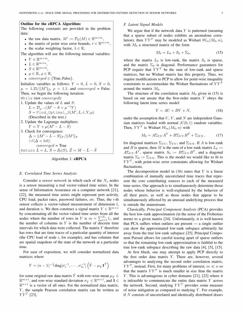
Outline for the eRPCA Algorithm:The following constants are provided in the problemdata:• the raw data matrix, M ′ := PΩ(M) ∈ Rm×m,• the matrix of point wise error bounds, ε ∈ Rm×m,• the scalar weighting factor, λ ∈ R,

The algorithm will use the following internal variables:• Y ∈ Rm×m,• L ∈ Rm×n,• S ∈ Rm×m,• µ ∈ R, ρ ∈ R,• converged ∈ True,False.

Initialize variables as follows: Y = 0, L = 0, S = 0,µ = 1.25/‖M ′‖2, ρ = 1.1, and converged = False.Then, we begin the following iteration:While (not converged):1. Update the values of L and S:

L = Dµ−1(M ′ − S + µ−1Y )S = Find_Optimal_S(M ′, L, ε, Y, µ)(Described in the text.)

2. Update the Lagrange multipliers:Y = Y + µ(M ′ − L− S)

3. Check for convergence:∆ = ‖M ′ − L− S‖F /‖M ′‖FIf(∆ < tol):

converged = TrueReturn L = L, S = Sε(S), Z = M − L− S

Algorithm 1: eRPCA

E. Correlated Time Series Analysis

Consider a sensor network in which each of the Ns nodesis a sensor measuring a real vector-valued time series. In thesense of Information Assurance on a computer network [21],[22], the measured time series might represent port activity,CPU load, packet rates, password failures, etc. Thus, the i-thsensor collects a vector-valued measurement of dimension liand duration n. We then construct a signal matrix Y ∈ Rm×nby concatenating all the vector-valued time series from all thenodes where the number of rows in Y is m =

∑Ns

i=1 li, andthe number of columns in Y is the number of discrete timeintervals for which data were collected. The matrix Y thereforehas rows that are time traces of a particular quantity of interest(the CPU load of node i, for example), and has columns thatare spatial snapshots of the state of the network at a particulartime.

For ease of exposition, we will consider normalized datamatrices where

Y = (n− 1)−12 diag[σ−1

1 , · · · , σ−1m ](Y − µY 1T

)for some original raw data matrix Y with row-wise mean µY ∈Rm×1, and row-wise standard deviation σY ∈ Rm×1, and 1 ∈Rn×1 is a vector of all ones. For the normalized data matrix,Y , the sample Pearson correlation matrix can be written asY Y T [23].

F. Latent Signal Models

We argue that if the network data Y is patterned (meaningthat a sparse subset of nodes exhibits an anomalous corre-lation), then Y Y T may be modeled as Wishart Wm(M0, n),with M0 a structured matrix of the form

M0 = L0 + S0 + Σ0, (15)

where the matrix L0 is low-rank, the matrix S0 is sparse,and the matrix Σ0 is diagonal. Performance guarantees forPCP require that Y Y T be the sum of low-rank and sparsematrices, but no Wishart matrix has this property. Thus, werequire modifications to PCP to allow for point-wise inequalityconstraints to accommodate the Wishart fluctuations of Y Y T

around the matrix M0.The structure of the correlation matrix M0 given in (15) is

based on our ansatz that the first-order matrix Y obeys thefollowing latent time series model:

Y = AU +BV +N, (16)

under the assumption that U , V , and N are independent Gaus-sian matrices loaded with normal N (0, 1) random variables.Then, Y Y T is Wishart Wm(M0, n) with

M0 = AΣUUAT +BΣV VB

T + ΣNN , (17)

for diagonal matrices ΣUU , ΣV V , and ΣNN . If A is low-rankand B is sparse, then M is the sum of a low-rank matrix L0 :=AΣUUA

T , sparse matrix S0 := BΣV VBT , and a diagonal

matrix Σ0 := ΣNN . This is the model we would like to fit toY Y T , with point-wise error constraints allowing for Wishartfluctuations.

The decomposition model in (16) states that Y is a linearcombination of mutually uncorrelated time traces that repre-sent the core contributing sources to each of the measuredtime series. Our approach is to simultaneously determine thosenodes whose behavior is well-explained by the behavior ofall their peers, as well as those nodes that appear to besimultaneously affected by an unusual underlying process thatis outside the mainstream.

Classically, Principal Component Analysis (PCA) providesthe best low-rank approximation (in the sense of the Frobeniusnorm) to a given matrix [24]. Unfortunately, it is well-knownthat PCA suffers when outliers are present — a single outliercan skew the approximated low-rank subspace arbitrarily faraway from the true low-rank subspace [25]. Principal Compo-nent Pursuit allows for careful teasing apart of sparse outliersso that the remaining low-rank approximation is faithful to thetrue low-rank subspace describing the raw data [4], [5], [15].

At first blush, one may attempt to apply PCP directly tothe first order data matrix Y . There are, however, severaladvantages to analyzing the second order correlation matrix,Y Y T , instead. First, for many problems of interest, m n sothat the matrix Y Y T is much smaller in size than the matrixY . This is advantageous in cyber domains [21], [22] where itis infeasible to communicate the entire data matrix Y acrossthe network. Second, studying Y Y T provides some measureof noise mitigation as compared to studying Y . For example,if N consists of uncorrelated and identically distributed draws

6 JOURNAL OF SELECTED TOPICS IN SIGNAL PROCESSING, VOL. 6, NO. 1, JANUARY 2013

from a zero mean, unit variance Gaussian distribution, then1nNN

T is Wishart Wm(I, n) with diagonal entries of unitmean and variance 1

n , and off-diagonal entries of zero meanand variance 1

n . In effect, the matrix ΣNN is an identity matrixwith Wishart fluctuations that are smaller than the fluctuationsin the original data Y .

Our analysis decomposes M = Y Y T into a low-rank partthat indicates the presence of a pervasive low-dimensionalpattern affecting the entire network, and a sparse part thatindicates sparse correlations between a few nodes that areanomalous when compared to the ambient background cor-relation.

In this approach, the role of the projection operator, PΩ,bears further comment. Recall from our earlier discussion onthe latent signal model that the error matrix Z0 is WishartWm(ΣNN , n) for diagonal matrix ΣNN . Any point-wise con-trol of the entries in Z0 should allow for larger point-wiseerrors on the diagonals where ΣNN is large. Since ΣNN isunknown, we proceed by removing the diagonal entries fromconsideration by adding the diagonal to the set of unobservedentries in Ω. That is, we expect M to be close to the sumof a low-rank matrix and a sparse matrix on the off-diagonalentries and allow the matrix completion algorithm to providethe unknown entries on the diagonal.

In the context of sensor networks, the introduction of entry-wise error control in (6) is motivated by the reality that we mayreceive data from heterogeneous sensors, and consequently, wemay wish to ascribe different error tolerances to each sensor,each sensor pair (for the second-order matrix), or to eachindividual measurement.

We emphasize that the proposed algorithm is intended toreveal anomalous temporal correlations between time signals;a situation where the signals at a small number of nodesall contain a component that is not felt anywhere else onthe network. Large values in S returned by the algorithmindicate that during the time interval under examination, asparse correlation occurred on that set of sensors. Moreover,the algorithm cannot identify at which moment during thattime interval the anomaly occurred. Indeed, the anomalydetected by the algorithm may arise from a diffuse signal thatoccurs unobtrusively throughout the entire time interval and istherefore not localized in time.

III. RESULTS AND DISCUSSION

A. Tests on Synthetic Data

To judge the performance of our algorithm we compare itto the Frobenius norm based formulation (5) presented in [5].We closely follow the test procedure in [5] by constructing anoise matrix Z0, a low-rank matrix L0, and a sparse matrixS0 as follows. The noise matrix Z0 ∈ Rn×n has entries whichare i.i.d. N(0, σ2) for a prescribed noise standard deviation σ.We construct the rank-r matrix L0 = U0V0 using U0 ∈ Rn×rand V0 ∈ Rr×n with i.i.d. entries from N(0, σ2

n) where, as in[5], we choose σn = 10 σ√

n. As noted in [5], this choice for σn

makes the singular values of L0 large compared to the singularvalues of Z0. Finally, we construct the sparse anomaly matrixS0 ∈ Rn×n with independently distributed entries, each being

zero with probability 1 − ρs, and uniform i.i.d. in the range[−5, 5] with probability ρs.

To compare (5) and (6), we use an accelerated proximalgradient method [26] to solve a dual version of (5) as

minL,S‖L‖∗ + λ‖S‖1 +

1

2µd‖M − L− S‖2F (18)

(see [5] for details), and Algorithm 1 for solving (6).As we use a fast ADMM method for (6), the computational

cost of our method is quite competitive when compared to theproximal gradient method for (5). Quantitative comparisonsof computational time are somewhat difficult, as the proximalgradient solver we use it written in Matlab [26] and ourADMM solver is written in C++. On a virtual machine usinga 2 GHz QEMU Virtual CPU version 1.0 processor, the runtime for the two algorithms is generally within a factor oftwo of each other, with the more efficient algorithm changingbased upon the exact problem one is solving. For one example,the ADMM algorithm uses approximately 42 seconds of CPUtime, while the proximal gradient algorithm uses approxi-mately 69 seconds. On another example, the ADMM algo-rithm uses approximately 43 seconds of CPU time, while theproximal gradient algorithm uses approximately 25 secondsof CPU time. Of course, these numbers vary based upon theiteration count for the two algorithms. The most expensivecomputation for both algorithms is an SVD decomposition ateach iteration, so it is not surprising that their computationalcosts are similar. We also observe both algorithms can beaccelerated using partial SVD algorithms.

Both (5) and (6) require judicious choice of parameters torecover L0 and S0 well. In particular, the dual version of(5) requires a choice of coupling constant, µd, between theobjective and the Frobenius constraint, and we follow [5] bychoosing µd =

√2nσ. Similarly, Algorithm 1 requires choice

of the point-wise constraint matrix ε. The goal of Algorithm1 is to allow the user flexibility in setting ε based upon thestructure of the problem. In particular, the user may set everyentry of ε differently to encode the knowledge they have oftheir problem. As (5) does not afford this flexibility we, forthe moment, choose a fixed value for all of the entries in ε asεij = 0.67σ. In this way, half of the total probability mass forthe Gaussian noise is in the range [−εij , εij ] and half of theprobability mass is outside that range.

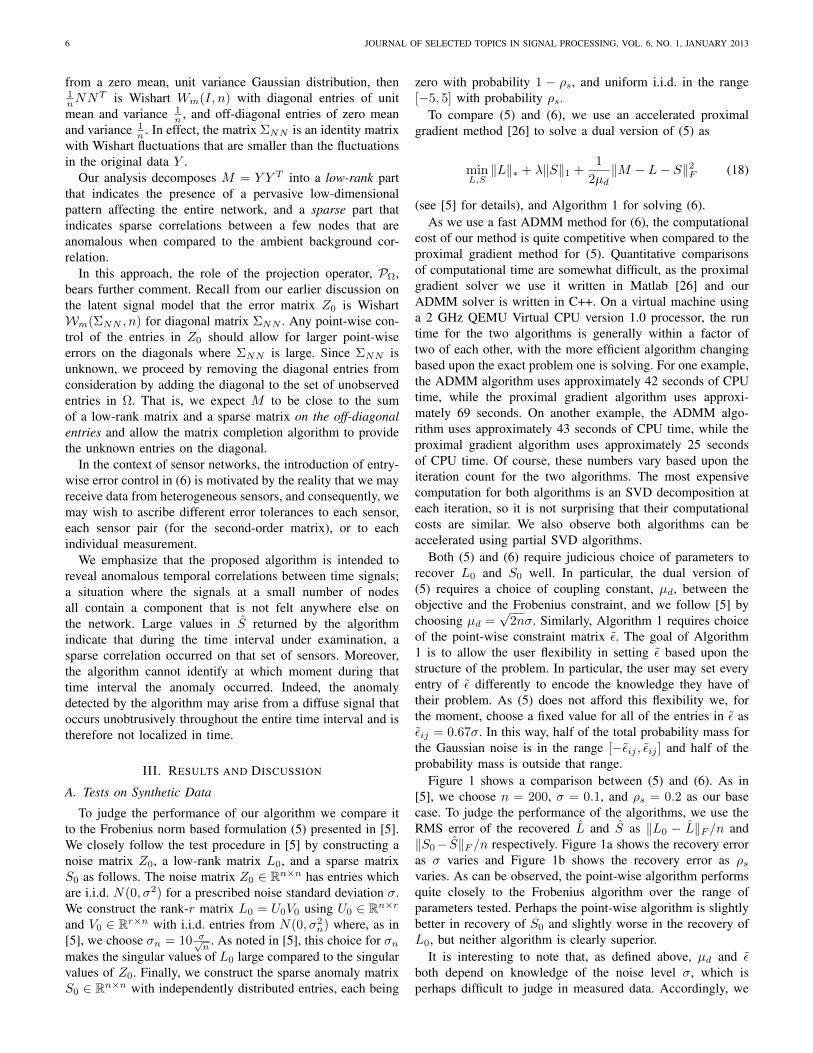
Figure 1 shows a comparison between (5) and (6). As in[5], we choose n = 200, σ = 0.1, and ρs = 0.2 as our basecase. To judge the performance of the algorithms, we use theRMS error of the recovered L and S as ‖L0 − L‖F /n and‖S0− S‖F /n respectively. Figure 1a shows the recovery erroras σ varies and Figure 1b shows the recovery error as ρsvaries. As can be observed, the point-wise algorithm performsquite closely to the Frobenius algorithm over the range ofparameters tested. Perhaps the point-wise algorithm is slightlybetter in recovery of S0 and slightly worse in the recovery ofL0, but neither algorithm is clearly superior.

It is interesting to note that, as defined above, µd and εboth depend on knowledge of the noise level σ, which isperhaps difficult to judge in measured data. Accordingly, we

PAFFENROTH et al.: SPACE-TIME SIGNAL PROCESSING FOR DISTRIBUTED PATTERN DETECTION IN SENSOR NETWORKS 7

(a) σ (b) ρs

Fig. 1. These figures show the RMS error in the recovery of L0

and S0, as a function of σ on the left and ρs on the right, whenthe correct σ is reported to both the Frobenius algorithm and thepoint-wise algorithm.

have generalized the testing procedure in [5] by consideringthe sensitivity of the algorithms to inaccurately known noise.

Figure 2 shows a similar experiment to Figure 1 except thetrue σ is twice as large as the σ reported to the algorithm forsetting µ or ε. In this case, the two algorithms are also roughlyequivalent. The idea is that the noise is sufficiently large sothat neither constraint can properly account for it. Accordingly,the noise corrupts both L and S for both algorithms.

(a) σ (b) ρs

Fig. 2. These figures show the RMS error in the recovery of L0

and S0, as a function of σ on the left and ρs on the right, whenan incorrect σ is reported to both the Frobenius algorithm and thepoint-wise algorithm. In this case the actual noise is two times largerthan what would be indicated by the reported σ.

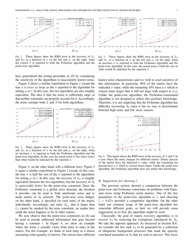
Figure 3, on the other hand, tells a different story. Figure 3is again a similar experiment to Figure 1 except, in this case,the true σ is half the size of the σ reported to the algorithmsfor setting µ or ε. In this case, the recovery of L0 is roughlyequivalent between the two algorithms, but the recovery of S0

is appreciably better for the point-wise constraint. Since theFrobenius constraint is a global error measure, the freedomit provides can be used to both ameliorate noise and tomask entries in S0 globally. The point-wise error budget,on the other hand, is specified for each entry of the matrixindividually. Accordingly, any entry S0ij that is larger thanεij cannot be masked by the error constraint, no matter howsmall the noise happens to be in other entries.

We now observe that the point-wise constraints in (6) canbe used to encode additional information that goes beyondhaving a constant ε. In Figure 4, we show an examplewhere the noise σ actually varies from entry to entry in thematrix. For this example, we think of each entry as a sensormeasuring some quantity of interest. The sensors have different

(a) σ (b) ρs

Fig. 3. These figures show the RMS error in the recovery of L0

and S0, as a function of σ on the left and ρs on the right, whenan incorrect σ is reported to both the Frobenius algorithm and thepoint-wise algorithm. In this case, the actual noise is half the size ofwhat would be indicated by the reported σ.

known noise characteristics and we wish to avail ourselves ofthis information. In particular, 90% of the entries have theindicated σ value, while the remaining 10% have a σ which issixteen times larger (but is still not large with respect to L0).Unlike the point-wise algorithm, the Frobenius-constrainedalgorithm is not designed to utilize this auxiliary knowledge.Therefore, it is not surprising that the Frobenius algorithm hasdifficulty recovering S0 since it has no way to discriminatebetween high noise and low noise sensors.

Fig. 4. This figure shows the RMS error in the recovery of L and S ina case where the noise changes for different entries. Ninety percentof the entries have the indicated σ value, while the remaining tenpercent have a σ which is sixteen times larger. Unlike the point-wisealgorithm, the Frobenius algorithm does not utilize this knowledge.

B. Suggestions for choosing ε

The previous section showed a comparison between thepoint-wise and Frobenius constraints on problems with Gaus-sian noise using Frobenius norm metrics. One of the keyparameters in the point-wise algorithm is ε, and choosingε = 0.67σ provides a competitive algorithm. On the otherhand, our common usage of the point-wise algorithm hassomewhat different goals, so here we will provide somesuggestions as to how the algorithm might be used.

Classically, the goal of matrix recovery algorithms is torecover L0 by removing the corruptions introduced by S0.We take the opposite approach. As discussed in Section II-F,we consider the low rank L0 to be generated by a collectionof ubiquitous background processes that mask the sparselycorrelated anomalies in S0 that we seek to uncover. This focus

8 JOURNAL OF SELECTED TOPICS IN SIGNAL PROCESSING, VOL. 6, NO. 1, JANUARY 2013

can be be seen in the previous section, where our recovery ofS0 is almost always better using the point-wise error constraintinstead of the Frobenius constraint.

Furthermore, we are often less concerned about the valuesin the recovered S than we are about detecting the support ofS0. As we will demonstrate in the next section, the supportof S in our second-order matrices is indicative of the sparsecorrelations that we wish to detect. With this in mind, inour work we often choose ε to be quite large. The idea isto capture the majority of the noise in the error constraint,thereby making the support of S less contaminated by noise.Of course, there is a trade-off. An ε which is very large formany entries of M0 not only ameliorates the noise, it alsoallows L to stray far from L0. Accordingly, our heuristic isto choose ε larger than our estimate for the noise, but not solarge that it tends to dominate L0.

C. Tests on Measured DataIn this section, we apply our algorithms for detecting

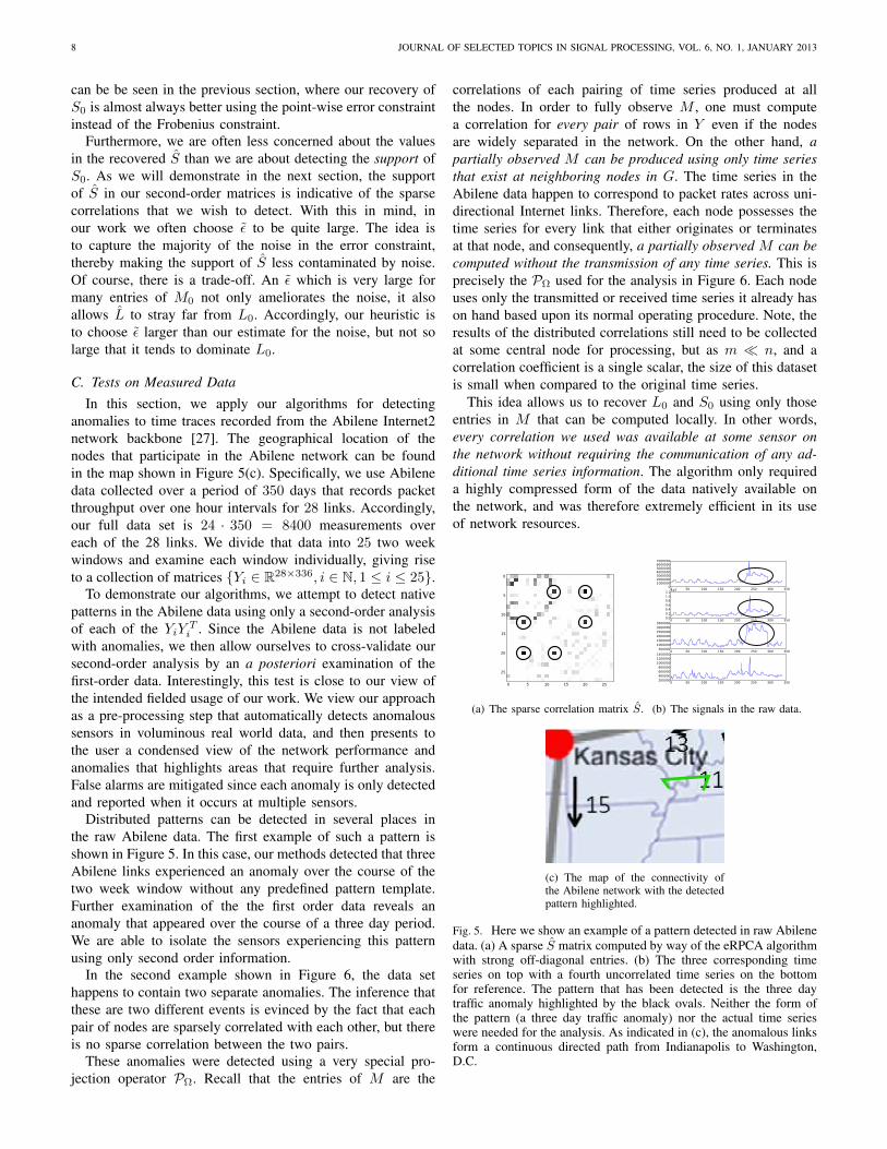
anomalies to time traces recorded from the Abilene Internet2network backbone [27]. The geographical location of thenodes that participate in the Abilene network can be foundin the map shown in Figure 5(c). Specifically, we use Abilenedata collected over a period of 350 days that records packetthroughput over one hour intervals for 28 links. Accordingly,our full data set is 24 · 350 = 8400 measurements overeach of the 28 links. We divide that data into 25 two weekwindows and examine each window individually, giving riseto a collection of matrices Yi ∈ R28×336, i ∈ N, 1 ≤ i ≤ 25.

To demonstrate our algorithms, we attempt to detect nativepatterns in the Abilene data using only a second-order analysisof each of the YiY

Ti . Since the Abilene data is not labeled

with anomalies, we then allow ourselves to cross-validate oursecond-order analysis by an a posteriori examination of thefirst-order data. Interestingly, this test is close to our view ofthe intended fielded usage of our work. We view our approachas a pre-processing step that automatically detects anomaloussensors in voluminous real world data, and then presents tothe user a condensed view of the network performance andanomalies that highlights areas that require further analysis.False alarms are mitigated since each anomaly is only detectedand reported when it occurs at multiple sensors.

Distributed patterns can be detected in several places inthe raw Abilene data. The first example of such a pattern isshown in Figure 5. In this case, our methods detected that threeAbilene links experienced an anomaly over the course of thetwo week window without any predefined pattern template.Further examination of the the first order data reveals ananomaly that appeared over the course of a three day period.We are able to isolate the sensors experiencing this patternusing only second order information.

In the second example shown in Figure 6, the data sethappens to contain two separate anomalies. The inference thatthese are two different events is evinced by the fact that eachpair of nodes are sparsely correlated with each other, but thereis no sparse correlation between the two pairs.

These anomalies were detected using a very special pro-jection operator PΩ. Recall that the entries of M are the

correlations of each pairing of time series produced at allthe nodes. In order to fully observe M , one must computea correlation for every pair of rows in Y even if the nodesare widely separated in the network. On the other hand, apartially observed M can be produced using only time seriesthat exist at neighboring nodes in G. The time series in theAbilene data happen to correspond to packet rates across uni-directional Internet links. Therefore, each node possesses thetime series for every link that either originates or terminatesat that node, and consequently, a partially observed M can becomputed without the transmission of any time series. This isprecisely the PΩ used for the analysis in Figure 6. Each nodeuses only the transmitted or received time series it already hason hand based upon its normal operating procedure. Note, theresults of the distributed correlations still need to be collectedat some central node for processing, but as m n, and acorrelation coefficient is a single scalar, the size of this datasetis small when compared to the original time series.

This idea allows us to recover L0 and S0 using only thoseentries in M that can be computed locally. In other words,every correlation we used was available at some sensor onthe network without requiring the communication of any ad-ditional time series information. The algorithm only requireda highly compressed form of the data natively available onthe network, and was therefore extremely efficient in its useof network resources.

0 5 10 15 20 25

0

5

10

15

20

25

(a) The sparse correlation matrix S.

0 50 100 150 200 250 300 3500

1000000200000030000004000000500000060000007000000

0 50 100 150 200 250 300 3500.00.20.40.60.81.01.2

1e7

0 50 100 150 200 250 300 350500000

100000015000002000000250000030000003500000

0 50 100 150 200 250 300 350200000400000600000800000100000012000001400000

(b) The signals in the raw data.

(c) The map of the connectivity ofthe Abilene network with the detectedpattern highlighted.

Fig. 5. Here we show an example of a pattern detected in raw Abilenedata. (a) A sparse S matrix computed by way of the eRPCA algorithmwith strong off-diagonal entries. (b) The three corresponding timeseries on top with a fourth uncorrelated time series on the bottomfor reference. The pattern that has been detected is the three daytraffic anomaly highlighted by the black ovals. Neither the form ofthe pattern (a three day traffic anomaly) nor the actual time serieswere needed for the analysis. As indicated in (c), the anomalous linksform a continuous directed path from Indianapolis to Washington,D.C.

PAFFENROTH et al.: SPACE-TIME SIGNAL PROCESSING FOR DISTRIBUTED PATTERN DETECTION IN SENSOR NETWORKS 9

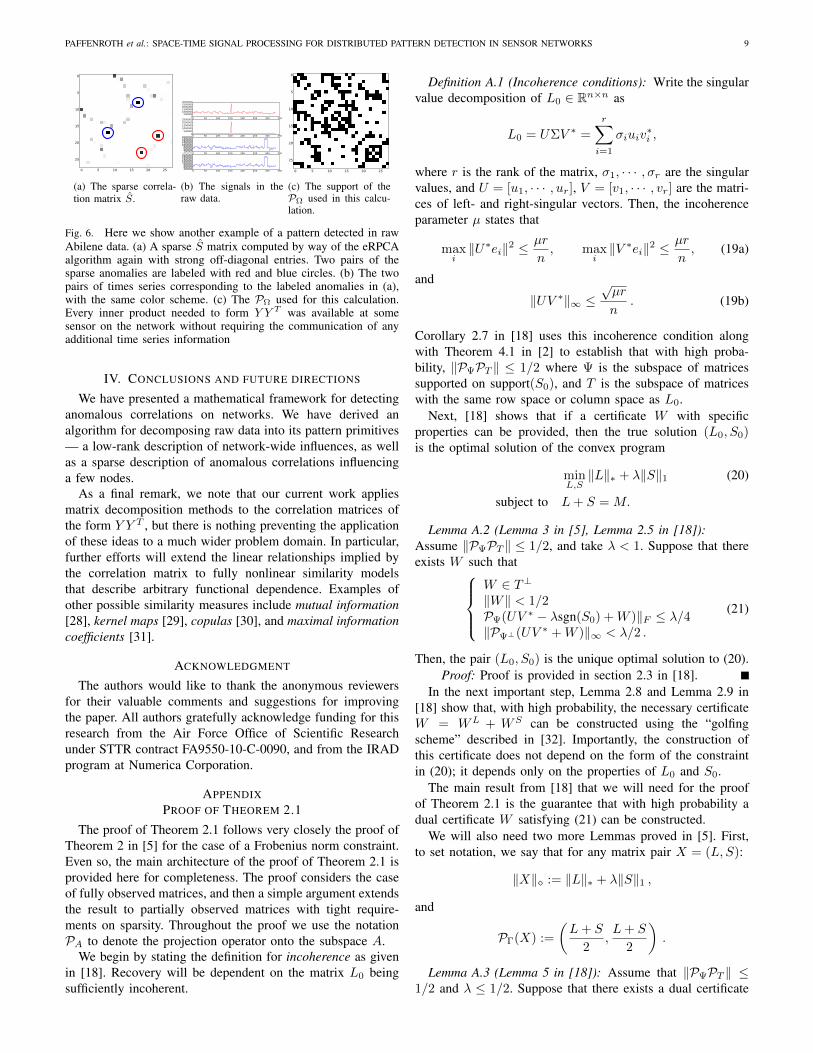
(a) The sparse correla-tion matrix S.

(b) The signals in theraw data.

(c) The support of thePΩ used in this calcu-lation.

Fig. 6. Here we show another example of a pattern detected in rawAbilene data. (a) A sparse S matrix computed by way of the eRPCAalgorithm again with strong off-diagonal entries. Two pairs of thesparse anomalies are labeled with red and blue circles. (b) The twopairs of times series corresponding to the labeled anomalies in (a),with the same color scheme. (c) The PΩ used for this calculation.Every inner product needed to form Y Y T was available at somesensor on the network without requiring the communication of anyadditional time series information

IV. CONCLUSIONS AND FUTURE DIRECTIONS

We have presented a mathematical framework for detectinganomalous correlations on networks. We have derived analgorithm for decomposing raw data into its pattern primitives— a low-rank description of network-wide influences, as wellas a sparse description of anomalous correlations influencinga few nodes.

As a final remark, we note that our current work appliesmatrix decomposition methods to the correlation matrices ofthe form Y Y T , but there is nothing preventing the applicationof these ideas to a much wider problem domain. In particular,further efforts will extend the linear relationships implied bythe correlation matrix to fully nonlinear similarity modelsthat describe arbitrary functional dependence. Examples ofother possible similarity measures include mutual information[28], kernel maps [29], copulas [30], and maximal informationcoefficients [31].

ACKNOWLEDGMENT

The authors would like to thank the anonymous reviewersfor their valuable comments and suggestions for improvingthe paper. All authors gratefully acknowledge funding for thisresearch from the Air Force Office of Scientific Researchunder STTR contract FA9550-10-C-0090, and from the IRADprogram at Numerica Corporation.

APPENDIXPROOF OF THEOREM 2.1

The proof of Theorem 2.1 follows very closely the proof ofTheorem 2 in [5] for the case of a Frobenius norm constraint.Even so, the main architecture of the proof of Theorem 2.1 isprovided here for completeness. The proof considers the caseof fully observed matrices, and then a simple argument extendsthe result to partially observed matrices with tight require-ments on sparsity. Throughout the proof we use the notationPA to denote the projection operator onto the subspace A.

We begin by stating the definition for incoherence as givenin [18]. Recovery will be dependent on the matrix L0 beingsufficiently incoherent.

Definition A.1 (Incoherence conditions): Write the singularvalue decomposition of L0 ∈ Rn×n as

L0 = UΣV ∗ =

r∑i=1

σiuiv∗i ,

where r is the rank of the matrix, σ1, · · · , σr are the singularvalues, and U = [u1, · · · , ur], V = [v1, · · · , vr] are the matri-ces of left- and right-singular vectors. Then, the incoherenceparameter µ states that

maxi‖U∗ei‖2 ≤

µr

n, max

i‖V ∗ei‖2 ≤

µr

n, (19a)

and

‖UV ∗‖∞ ≤√µr

n. (19b)

Corollary 2.7 in [18] uses this incoherence condition alongwith Theorem 4.1 in [2] to establish that with high proba-bility, ‖PΨPT ‖ ≤ 1/2 where Ψ is the subspace of matricessupported on support(S0), and T is the subspace of matriceswith the same row space or column space as L0.

Next, [18] shows that if a certificate W with specificproperties can be provided, then the true solution (L0, S0)is the optimal solution of the convex program

minL,S‖L‖∗ + λ‖S‖1 (20)

subject to L+ S = M.

Lemma A.2 (Lemma 3 in [5], Lemma 2.5 in [18]):Assume ‖PΨPT ‖ ≤ 1/2, and take λ < 1. Suppose that thereexists W such that

W ∈ T⊥‖W‖ < 1/2PΨ(UV ∗ − λsgn(S0) +W )‖F ≤ λ/4‖PΨ⊥(UV ∗ +W )‖∞ < λ/2 .

(21)

Then, the pair (L0, S0) is the unique optimal solution to (20).Proof: Proof is provided in section 2.3 in [18].

In the next important step, Lemma 2.8 and Lemma 2.9 in[18] show that, with high probability, the necessary certificateW = WL + WS can be constructed using the “golfingscheme” described in [32]. Importantly, the construction ofthis certificate does not depend on the form of the constraintin (20); it depends only on the properties of L0 and S0.

The main result from [18] that we will need for the proofof Theorem 2.1 is the guarantee that with high probability adual certificate W satisfying (21) can be constructed.

We will also need two more Lemmas proved in [5]. First,to set notation, we say that for any matrix pair X = (L, S):

‖X‖ := ‖L‖∗ + λ‖S‖1 ,

and

PΓ(X) :=

(L+ S

2,L+ S

2

).

Lemma A.3 (Lemma 5 in [18]): Assume that ‖PΨPT ‖ ≤1/2 and λ ≤ 1/2. Suppose that there exists a dual certificate

10 JOURNAL OF SELECTED TOPICS IN SIGNAL PROCESSING, VOL. 6, NO. 1, JANUARY 2013

W satisfying (21) and write Λ = UV ∗ + W . Then for anyperturbation, H = (HL, HS) obeying HL +HS = 0,

‖X0 +H‖ ≥‖X0‖ + (3/4− ‖PT⊥(Λ)‖) ‖PT⊥(HL)‖∗+ (3λ/4− ‖PΨ⊥(Λ)‖∞) ‖PΨ⊥(HS)‖1 .

Lemma A.4 (Lemma 6 in [18]): Suppose that ‖PTPΨ‖ ≤1/2. Then for any pair X := (L, S),

‖(PT × PΨ)(X)‖2F ≤ 4‖PΓ(PT × PΨ)(X)‖2F .

We are now prepared to state our main proposition:Proposition A.5 (Modification of Proposition 4 in [5]):

Assume ‖PΨPT ‖ ≤ 1/2, λ ≤ 1/2, and that there exists adual certificate W satisfying (21). Let X = (L, S) be thesolution to (6), and X0 := (L0, S0); then X satisfies

‖X0 − X‖F ≤ (8√

5n+√

2)δ .

Proposition A.5 implies Theorem 2.1, since under the con-ditions of Theorem 2.1, the results cited in [18] show that withhigh probability there indeed exists a dual certificate W thatsatisfies (21), and Corollary 2.7 of [18] proves ‖PΨPT ‖ ≤ 1/2as well. Importantly, we see that we can very quickly usethis result to demonstrate stable recovery for the case of apartially observed M0. We do so by regarding the unobservedentries of M0 as corruptions (non-zero entries in S0), and thenapplying the theorem for fully observed matrices where therequirements on the sparsity of the support of S0 must alsoinclude the support of the unobserved entries.

Finally, we proceed to the proof of Proposition A.5 whichuses the same arguments as [5].

Proof: Our algorithm is stable if the error differencebetween truth, X0 := (L0, S0), and our recovery, X := (L, S),is bounded by the size of the noise. To quantify this error, wedefine

H := (HL, HS) := X −X0 .

Since X minimizes the optimization problem in (6), and X0

is also a feasible solution to the optimization, it is necessarilytrue that

‖X‖ ≤ ‖X0‖ . (22)

Second, using the triangle inequality,

‖L+ S − L0 − S0‖F ≤ ‖L+ S −M‖F + ‖L0 + S0 −M‖F≤ ‖L+ S −M‖1 + ‖L0 + S0 −M‖1≤ ‖ε‖1 + ‖Z0‖1≤ 2δ . (23)

Our end goal is to bound the size of

‖H‖2F = ‖HL‖2F + ‖HS‖2F = ‖L− L0‖2F + ‖S − S0‖2F

by a term that goes to zero as the size of the noise goes tozero. To achieve this, we seek to control

‖H‖2F = ‖HΓ‖2F + ‖HΓ⊥‖2F .

We begin by bounding the first term using (23) as follows:

‖HΓ‖2F =

∥∥∥∥HL +HS

2

∥∥∥∥2

F

+

∥∥∥∥HL +HS

2

∥∥∥∥2

F

=1

2‖HL +HS‖2F

=1

2‖L− L0 + S − S0‖2F

≤ 2δ2 . (24)

All that remains is to bound the term ‖HΓ⊥‖2F . Again, wedivide this term into two terms using orthogonal projections:

‖HΓ⊥‖2F =‖(PT × PΨ)(HΓ⊥)‖2F+ ‖(PT⊥ × PΨ⊥)(HΓ⊥)‖2F , (25)

and bound the terms independently.First, consider ‖(PT⊥ × PΨ⊥)(HΓ⊥)‖2F . Let W be a dual

certificate satisfying (21). Then, Λ := UV ∗ + W obeys‖PT⊥(Λ)‖ ≤ 1

2 and ‖PΨ⊥(Λ)‖∞ ≤ λ2 . By the triangle

inequality, and the bound ‖X‖ ≤ ‖X0‖ obtained in (22),we have

‖X0 +HΓ⊥‖ ≤ ‖X0 +H‖ + ‖HΓ‖= ‖X‖ + ‖HΓ‖≤ ‖X0‖ + ‖HΓ‖ . (26)

Also, by Lemma A.3, we have

‖X0 +HΓ⊥‖≥‖X0‖ + (3/4− ‖PT⊥(Λ)‖)‖PT⊥(HΓ⊥

L )‖∗+ (3λ/4− ‖PΨ⊥(Λ)‖∞)‖PΨ⊥(HΓ⊥

S )‖1≥‖X0‖ + (3/4− 1/2)‖PT⊥(HΓ⊥

L )‖∗+ (3λ/4− λ/2)‖PΨ⊥(HΓ⊥

S )‖1≥‖X0‖ + 1/4‖PT⊥(HΓ⊥

L )‖∗ + λ/4‖PΨ⊥(HΓ⊥

S )‖1 (27)

where we have used the assumptions ‖PT⊥(Λ)‖ ≤ 12 and

‖PΨ⊥(Λ)‖∞ ≤ λ2 . Rearranging (27) yields

1/4‖PT⊥(HΓ⊥

L )‖∗ + λ/4‖PΨ⊥(HΓ⊥

S )‖1≤ ‖X0 +HΓ⊥‖ − ‖X0‖ . (28)

Taking the inequalities in (26) and (28) together implies that

‖PT⊥(HΓ⊥

L )‖∗ + λ‖PΨ⊥(HΓ⊥

S )‖1 ≤ 4‖HΓ‖. (29)

Note that by definition of HΓ,

‖HΓ‖F =

(∥∥∥∥HL +HS

2

∥∥∥∥2

F

+

∥∥∥∥HL +HS

2

∥∥∥∥2

F

) 12

=√

2

∥∥∥∥HL +HS

2

∥∥∥∥F

=√

2∥∥HΓ

L

∥∥F

=1√2

(∥∥HΓL

∥∥F

+∥∥HΓ

S

∥∥F

), (using HΓ

L = HΓS )

so that we can write,∥∥HΓL

∥∥F

+∥∥HΓ

S

∥∥F

=√

2‖HΓ‖F . (30)

PAFFENROTH et al.: SPACE-TIME SIGNAL PROCESSING FOR DISTRIBUTED PATTERN DETECTION IN SENSOR NETWORKS 11

Therefore,

‖(PT⊥ × PΨ⊥)(HΓ⊥)‖F≤ ‖PT⊥(HΓ⊥

L )‖F + ‖PΨ⊥(HΓ⊥

S )‖F≤ ‖PT⊥(HΓ⊥

L )‖∗ + λ√n‖PΨ⊥(HΓ⊥

S )‖1≤ 4√n‖HΓ‖ (using (29))

= 4√n(‖HΓ

L‖∗ + λ‖HΓS‖1)

≤ 4n(‖HΓL‖F + ‖HΓ

S‖F )

= 4√

2n‖HΓ‖F ≤ 8nδ , (using (30) and (24))

from which we may write

‖(PT⊥ × PΨ⊥)(HΓ⊥)‖2F ≤ 64n2δ2 . (31)

Now, we proceed to derive a bound for the first term in (25).By Lemma A.4,

‖(PT × PΨ)(HΓ⊥)‖2F ≤ 4‖PΓ(PT × PΨ)(HΓ⊥)‖2F . (32)

Also, since

PΓ(HΓ⊥) = 0 = PΓ(PT × PΨ)(HΓ⊥) + PΓ(PT⊥ × PΨ⊥)(HΓ⊥)

implies

PΓ(PT × PΨ)(HΓ⊥) = −PΓ(PT⊥ × PΨ⊥)(HΓ⊥),

we have

‖PΓ(PT × PΨ)(HΓ⊥)‖F = ‖PΓ(PT⊥ × PΨ⊥)(HΓ⊥)‖F≤ ‖(PT⊥ × PΨ⊥)(HΓ⊥)‖F .

(33)

Combining the previous two inequalities in (32) and (33), wehave

‖(PT × PΨ)(HΓ⊥)‖2F ≤ 4‖(PT⊥ × PΨ⊥)(HΓ⊥)‖2F ,

which together with (31) yields

‖(PT × PΨ)(HΓ⊥)‖2F ≤ 4 · 64n2δ2 . (34)

Combining the bounds obtained in (31) and (34), we have

‖HΓ⊥‖2F = ‖(PT × PΨ)(HΓ⊥)‖2F + ‖(PT⊥ × PΨ⊥)(HΓ⊥)‖2F≤ 4 · 64n2δ2 + 64n2δ2

= 5 · 64n2δ2 . (35)

Finally, using (24) and (35), the bound on the total errorbecomes

‖H‖2F = ‖HΓ‖2F + ‖HΓ⊥‖2F≤ 2δ2 + 5 · 64n2δ2 (36)

which yields

‖X0 − X‖F = ‖H‖F≤√

2δ2 + 5 · 64n2δ2 (by (36))

≤ (√

2 + 8√

5n)δ ,

and we have shown that the error term is bounded linearly inδ as desired for Proposition A.5.

REFERENCES

[1] E. Candes, J. Romberg, and T. Tao, “Robust uncertaintyprinciples: exact signal reconstruction from highly incompletefrequency information,” IEEE Transactions on InformationTheory, vol. 52, no. 2, pp. 489–509, 2006. [Online]. Available:http://ieeexplore.ieee.org/lpdocs/epic03/wrapper.htm?arnumber=1580791

[2] E. J. Candes and B. Recht, “Exact matrix completion via convexoptimization,” Foundations of Computational Mathematics, vol. 9, no. 6,pp. 717–772, December 2009.

[3] V. Chandrasekaran, S. Sanghavi, P. Parrilo, and A. Willsky, “Rank-sparsity incoherence for matrix decomposition,” SIAM Journal onOptimization, vol. 21, no. 2, pp. 572–596, 2011. [Online]. Available:http://epubs.siam.org/doi/abs/10.1137/090761793

[4] E. J. Candes, X. Li, Y. Ma, and J. Wright, “Robust principal componentanalysis?” J. ACM, vol. 58, no. 3, pp. 11:1–11:37, Jun. 2011. [Online].Available: http://doi.acm.org/10.1145/1970392.1970395

[5] Z. Zhou, X. Li, J. Wright, E. Candes, and Y. Ma, “Stable PrincipalComponent Pursuit,” ISIT 2010: Proceedings of IEEE InternationalSymposium on Information Technology, 2010. [Online]. Available:http://perception.csl.illinois.edu/matrix-rank/Files/isit noise.pdf

[6] V. Chandrasekaran, B. Recht, P. A. Parrilo, and A. S. Willsky, “Theconvex geometry of linear inverse problems,” To be submitted, December2010.

[7] R. Mikut and M. Reischl, “Data mining tools,” Wiley InterdisciplinaryReviews: Data Mining and Knowledge Discovery, vol. 1, no. 5, pp.431–443, 2011. [Online]. Available: http://dx.doi.org/10.1002/widm.24

[8] D. Haughton, J. Deichmann, A. Eshghi, S. Sayek, N. Teebagy, andH. Topi, “A review of software packages for data mining,” The AmericanStatistician, vol. 57, no. 4, pp. 290–309, November 2003.

[9] I. Witten, E. Frank, M. Hall, and G. Holmes, Data Mining: PracticalMachine Learning Tools and Techniques, ser. The Morgan KaufmannSeries in Data Management Systems. Elsevier Science, 2011. [Online].Available: http://books.google.com/books?id=bDtLM8CODsQC

[10] C. Bishop, Pattern Recognition And Machine Learning, ser.Information Science and Statistics. Springer, 2006. [Online]. Available:http://books.google.com/books?id=kTNoQgAACAAJ

[11] S. Marsland, Machine Learning: An Algorithmic Perspective,ser. Chapman & Hall/CRC machine learning & patternrecognition series. CRC Press, 2009. [Online]. Available:http://books.google.com/books?id=n66O8a4SWGEC

[12] S. Macskassy and F. Provost, “A brief survey of machine learningmethods for classification in networked data and an application tosuspicion scoring,” in Statistical Network Analysis: Models, Issues,and New Directions, ser. Lecture Notes in Computer Science,E. Airoldi, D. Blei, S. Fienberg, A. Goldenberg, E. Xing, andA. Zheng, Eds. Springer Berlin / Heidelberg, 2007, vol. 4503,pp. 172–175, 10.1007/978-3-540-73133-7 13. [Online]. Available:http://dx.doi.org/10.1007/978-3-540-73133-7 13

[13] C. Krugel and T. Toth, “Distributed pattern detection forintrusion detection,” in Proc. of the Network and DistributedSystem Security Symp. (NDSS 2002), 2002. [Online]. Available:http://citeseer.ist.psu.edu/kruegel02distributed.html

[14] N. Boggs, S. Hiremagalore, A. Stavrou, and S. Stolfo, “Cross-domaincollaborative anomaly detection: So far yet so close,” in Recent Advancesin Intrusion Detection 14th International Symposium, 2011.

[15] A. Ganesh, J. Wright, X. Li, E. Candes, and Y. Ma, “Dense errorcorrection for low-rank matrices via principal component pursuit,”in Information Theory Proceedings (ISIT), 2010 IEEE InternationalSymposium on, June 2010, pp. 1513 –1517.

[16] R. C. Paffenroth, P. C. Du Toit, L. L. Scharf, A. P. Jayasumana, V. W.Banadara, and R. Nong, “Space-time signal processing for distributedpattern detection in sensor networks,” in Society of Photo-OpticalInstrumentation Engineers (SPIE) Conference Series, ser. Society ofPhoto-Optical Instrumentation Engineers (SPIE) Conference Series, vol.8393. SPIE, May 2012.

[17] R. C. Paffenroth, P. C. Du Toit, L. L. Scharf, A. P. Jayasumana,V. W. Banadara, and R. Nong, “Distributed pattern detection incyber networks,” in Society of Photo-Optical Instrumentation Engineers(SPIE) Conference Series, ser. Society of Photo-Optical InstrumentationEngineers (SPIE) Conference Series, I. V. Ternovskiy and P. Chin,Eds., vol. 8408, no. 1. SPIE, 2012, p. 84080J. [Online]. Available:http://link.aip.org/link/?PSI/8408/84080J/1

[18] E. J. Candes and Y. Plan, “Matrix completion with noise,” Proceedingsof the IEEE, vol. 98, no. 6, pp. 925–936, Jun. 2010. [Online]. Available:http://ieeexplore.ieee.org/lpdocs/epic03/wrapper.htm?arnumber=5454406

12 JOURNAL OF SELECTED TOPICS IN SIGNAL PROCESSING, VOL. 6, NO. 1, JANUARY 2013

[19] S. Boyd, N. Parikh, E. Chu, B. Peleato, and J. Eckstein, DistributedOptimization and Statistical Learning Via the Alternating DirectionMethod of Multipliers. Now Publishers, 2011. [Online]. Available:http://books.google.com/books?id=8MjgLpJ0 4YC

[20] J.-F. Cai, E. J. Candes, and Z. Shen, “A singular value thresholdingalgorithm for matrix completion,” SIAM J. on Optimization,vol. 20, no. 4, pp. 1956–1982, Mar. 2010. [Online]. Available:http://dx.doi.org/10.1137/080738970

[21] D. B. Parker, Fighting computer crime: a new framework for protectinginformation. New York, NY, USA: John Wiley & Sons, Inc., 1998.

[22] ——, “Toward a New Framework for Information Security,” in Com-puter Security Handbook, 4th ed., S. Bosworth and M. E. Kabay, Eds.John Wiley and Sons, 2002, ch. 5.

[23] S. Boslaugh and P. Watters, Statistics in a Nutshell: A Desktop QuickReference, ser. In a Nutshell. O’Reilly, 2008. [Online]. Available:http://books.google.com/books?id=ZnhgO65Pyl4C

[24] C. Eckart and G. Young, “The approximation of one matrix by anotherof lower rank,” Psychometrika, vol. 1, no. 3, pp. 211–218, Sep. 1936.[Online]. Available: http://dx.doi.org/10.1007/BF02288367

[25] H. Ringberg, A. Soule, J. Rexford, and C. Diot, “Sensitivity of PCA fortraffic anomaly detection,” Proceedings of the 2007 ACM SIGMETRICSinternational conference on Measurement and modeling of computersystems SIGMETRICS 07, vol. 35, no. 1, p. 109, 2007. [Online].Available: http://portal.acm.org/citation.cfm?doid=1254882.1254895

[26] Z. Lin, A. Ganesh, J. Wright, L. Wu, M. Chen, , and Y. Ma, “Fast convexoptimization algorithms for exact recovery of a corrupted low-rankmatrix,” University of Illinois Urbana-Champaign, Tech. Rep. UILU-ENG-09-2214, August 2009.

[27] “Internet 2 network,” Web Page: http://noc.net.internet2.edu/i2network/index.html.[28] P. J. Schreier and L. L. Scharf, Statistical signal processing of complex-

valued data: the theory of improper and noncircular signals. CambridgeUniversity Press, 2010.

[29] A. Aizerman, E. M. Braverman, and L. I. Rozoner, “Theoretical founda-tions of the potential function method in pattern recognition learning,”Automation and Remote Control, vol. 25, pp. 821–837, 1964.

[30] R. Nelsen, An Introduction to Copulas, ser. SpringerSeries in Statistics. Springer, 2010. [Online]. Available:http://books.google.com/books?id=HhdjcgAACAAJ

[31] D. N. Reshef, Y. A. Reshef, H. K. Finucane, S. R. Grossman,G. McVean, P. J. Turnbaugh, E. S. Lander, M. Mitzenmacher,and P. C. Sabeti, “Detecting novel associations in large data sets,”Science, vol. 334, no. 6062, pp. 1518–1524, 2011. [Online]. Available:http://www.sciencemag.org/content/334/6062/1518.abstract

[32] D. Gross, “Recovering low-rank matrices from few coefficients in anybasis,” CoRR, vol. abs/0910.1879, 2009.

PLACEPHOTOHERE

Randy Paffenroth Biography will be inserted onacceptance of the paper.

PLACEPHOTOHERE

Philip Du Toit Biography will be inserted on ac-ceptance of the paper.

PLACEPHOTOHERE

Ryan Nong Biography will be inserted on accep-tance of the paper.

PLACEPHOTOHERE

Louis Scharf Biography will be inserted on accep-tance of the paper.

PLACEPHOTOHERE

Anura Jayasumana Biography will be inserted onacceptance of the paper.

PLACEPHOTOHERE

Vidarshana Bandara Biography will be inserted onacceptance of the paper.