Journal of Hydrology · Using discrete wavelet transforms to analyze trends in streamflow and...
25
Using discrete wavelet transforms to analyze trends in streamflow and precipitation in Quebec and Ontario (1954–2008) D. Nalley, J. Adamowski, B. Khalil ⇑ Department of Bioresource Engineering, Faculty of Agriculture and Environmental Sciences, McGill University, Macdonald Stewart Building, 21111 Lakeshore Road, Ste-Anne-de-Bellevue, Quebec, Canada H9X 3V9 article info Article history: Received 15 May 2012 Received in revised form 9 September 2012 Accepted 25 September 2012 Available online 4 October 2012 This manuscript was handled by Andras Bardossy, Editor-in-Chief, with the assistance of Efrat Morin, Associate Editor Keywords: Trend detection Streamflow Precipitation Discrete wavelet transform Mann–Kendall trend test summary This paper aims to detect trends in mean flow and total precipitation data over southern parts of Quebec and Ontario, Canada. The main purpose of the trend assessment is to find out what time scales are affect- ing the trends observed in the datasets used. In this study, a new trend detection method for hydrological studies is explored, which involves the use of wavelet transforms (WTs) in order to separate the rapidly and slowly changing events contained in a time series. More specifically, this study co-utilizes the Dis- crete Wavelet Transform (DWT) technique and the Mann–Kendall (MK) trend tests to analyze and detect trends in monthly, seasonally-based, and annual data from eight flow stations and seven meteorological stations in southern Ontario and Quebec during 1954–2008. The combination of the DWT and MK test in analyzing trends has not been extensively explored to date, especially in detecting trends in Canadian flow and precipitation time series. The mother wavelet type and the extension border used in the wavelet transform, as well as the number of decomposition levels, were determined based on two criteria. The first criterion is the mean relative error of the wavelet approximation series and the original time series. In addition, a new criterion is proposed and explored in this study, which is based on the relative error of the MK Z-values of the approximation component and the original time series. Sequential Mann–Kendall analysis on the different wavelet detail components (with their approximation component added) that result from the time series decomposition was also used and found to be helpful because it depicts how harmonious each of the detail components (plus approximation) is with respect to the original data. This study found that most of the trends are positive and started during the mid-1960s to early 1970s. The results from the wavelet analysis and Mann–Kendall tests on the different data types (using the 5% significance level) reveal that in general, intra- and inter-annual events (up to 4 years) are more influ- ential in affecting the observed trends. Ó 2012 Elsevier B.V. All rights reserved. 1. Introduction The intensification of the hydrologic cycle is one of the most evident effects caused by climate warming (Ampitiyawatta and Guo, 2009; Zhang et al., 2009; Durdu, 2010). Changes in hydrolog- ical processes may in turn affect the overall availability and quality of water resources, and alter the spatiotemporal characteristics of hydrologic occurrences, such as the timing of flow events, and the frequency and severity of floods and droughts (Mishra and Singh, 2010; Burn et al., 2010). High-latitude areas have been pro- jected to experience more severe impacts associated with climate change (Zhang et al., 2001). Labat et al. (2004) who studied the glo- bal and continental runoff associated with temperature increases found that North America is very vulnerable to recent climate change. One of the most significant consequences of temperature increases and changes in precipitation patterns is the dramatic modification of the hydrologic regimes of northern rivers (Boyer et al., 2010). The impacts of changing climate in Canada vary from one area to another and have been studied by numerous authors, both at the national and regional scale. Studies on trends of various hy- dro-climatic indices reveal a variety of results; both positive and negative trends were found across different parts of Canada. According to Ehsanzadeh et al. (2011), who analyzed Canadian low flows, there is a positive trend in winter low flows (including in eastern Canada), but the trends are negative in western Canada. Summer low flows are found to exhibit positive trends in central Canada, but the trends are negative in regions such as eastern On- tario and Quebec (Ehsanzadeh et al., 2011). Similarly, Adamowski and Bocci (2001) found that there is a significant positive trend in the yearly low flow in western Quebec and southern Ontario; 0022-1694/$ - see front matter Ó 2012 Elsevier B.V. All rights reserved. http://dx.doi.org/10.1016/j.jhydrol.2012.09.049 ⇑ Corresponding author. Tel.: +1 514 398 7614; fax: +1 514 398 8387. E-mail addresses: [email protected] (D. Nalley), jan.adamowski@mc- gill.ca (J. Adamowski), [email protected], [email protected] (B. Khalil). Journal of Hydrology 475 (2012) 204–228 Contents lists available at SciVerse ScienceDirect Journal of Hydrology journal homepage: www.elsevier.com/locate/jhydrol
Transcript of Journal of Hydrology · Using discrete wavelet transforms to analyze trends in streamflow and...

Journal of Hydrology 475 (2012) 204–228
Contents lists available at SciVerse ScienceDirect
Journal of Hydrology
journal homepage: www.elsevier .com/locate / jhydrol
Using discrete wavelet transforms to analyze trends in streamflowand precipitation in Quebec and Ontario (1954–2008)
D. Nalley, J. Adamowski, B. Khalil ⇑Department of Bioresource Engineering, Faculty of Agriculture and Environmental Sciences, McGill University, Macdonald Stewart Building, 21111 Lakeshore Road,Ste-Anne-de-Bellevue, Quebec, Canada H9X 3V9
a r t i c l e i n f o s u m m a r y
Article history:Received 15 May 2012Received in revised form 9 September 2012Accepted 25 September 2012Available online 4 October 2012This manuscript was handled by AndrasBardossy, Editor-in-Chief, with theassistance of Efrat Morin, Associate Editor
Keywords:Trend detectionStreamflowPrecipitationDiscrete wavelet transformMann–Kendall trend test
0022-1694/$ - see front matter � 2012 Elsevier B.V. Ahttp://dx.doi.org/10.1016/j.jhydrol.2012.09.049
⇑ Corresponding author. Tel.: +1 514 398 7614; faxE-mail addresses: [email protected] (D.
gill.ca (J. Adamowski), [email protected], b(B. Khalil).
This paper aims to detect trends in mean flow and total precipitation data over southern parts of Quebecand Ontario, Canada. The main purpose of the trend assessment is to find out what time scales are affect-ing the trends observed in the datasets used. In this study, a new trend detection method for hydrologicalstudies is explored, which involves the use of wavelet transforms (WTs) in order to separate the rapidlyand slowly changing events contained in a time series. More specifically, this study co-utilizes the Dis-crete Wavelet Transform (DWT) technique and the Mann–Kendall (MK) trend tests to analyze and detecttrends in monthly, seasonally-based, and annual data from eight flow stations and seven meteorologicalstations in southern Ontario and Quebec during 1954–2008. The combination of the DWT and MK test inanalyzing trends has not been extensively explored to date, especially in detecting trends in Canadianflow and precipitation time series. The mother wavelet type and the extension border used in the wavelettransform, as well as the number of decomposition levels, were determined based on two criteria. Thefirst criterion is the mean relative error of the wavelet approximation series and the original time series.In addition, a new criterion is proposed and explored in this study, which is based on the relative error ofthe MK Z-values of the approximation component and the original time series. Sequential Mann–Kendallanalysis on the different wavelet detail components (with their approximation component added) thatresult from the time series decomposition was also used and found to be helpful because it depictshow harmonious each of the detail components (plus approximation) is with respect to the original data.This study found that most of the trends are positive and started during the mid-1960s to early 1970s.The results from the wavelet analysis and Mann–Kendall tests on the different data types (using the5% significance level) reveal that in general, intra- and inter-annual events (up to 4 years) are more influ-ential in affecting the observed trends.
� 2012 Elsevier B.V. All rights reserved.
1. Introduction
The intensification of the hydrologic cycle is one of the mostevident effects caused by climate warming (Ampitiyawatta andGuo, 2009; Zhang et al., 2009; Durdu, 2010). Changes in hydrolog-ical processes may in turn affect the overall availability and qualityof water resources, and alter the spatiotemporal characteristics ofhydrologic occurrences, such as the timing of flow events, andthe frequency and severity of floods and droughts (Mishra andSingh, 2010; Burn et al., 2010). High-latitude areas have been pro-jected to experience more severe impacts associated with climatechange (Zhang et al., 2001). Labat et al. (2004) who studied the glo-bal and continental runoff associated with temperature increases
ll rights reserved.
: +1 514 398 8387.Nalley), jan.adamowski@[email protected]
found that North America is very vulnerable to recent climatechange. One of the most significant consequences of temperatureincreases and changes in precipitation patterns is the dramaticmodification of the hydrologic regimes of northern rivers (Boyeret al., 2010).
The impacts of changing climate in Canada vary from one areato another and have been studied by numerous authors, both atthe national and regional scale. Studies on trends of various hy-dro-climatic indices reveal a variety of results; both positive andnegative trends were found across different parts of Canada.According to Ehsanzadeh et al. (2011), who analyzed Canadianlow flows, there is a positive trend in winter low flows (includingin eastern Canada), but the trends are negative in western Canada.Summer low flows are found to exhibit positive trends in centralCanada, but the trends are negative in regions such as eastern On-tario and Quebec (Ehsanzadeh et al., 2011). Similarly, Adamowskiand Bocci (2001) found that there is a significant positive trendin the yearly low flow in western Quebec and southern Ontario;

D. Nalley et al. / Journal of Hydrology 475 (2012) 204–228 205
however, the opposite was observed for central and eastern Canadafor the same variable. The latest assessment by the Intergovern-mental Panel on Climate Change (IPCC) also stated that annual pre-cipitation has increased over much of North America, especially innorthern Canada, but has decreased in the Canadian Prairies (IPCC,2007). Recent changes in annual total precipitations in Canadawere between �10% and +35% (Zhang et al., 2001).
One of the predicted effects of climate change in Quebec is theincrease in the intensity and frequency of heavy floods, resultingfrom heavy precipitation (Assani et al., 2010). McBean and Motiee(2006) also found that there are significant upward trends at the5%-level in flow and precipitation for the Great Lakes watershedover the period of 1930–1990. These findings are relatively consis-tent with the predictions of the General Circulation Models (GCMs)for the year 2050 (McBean and Motiee, 2006). The results of theCanadian General Circulation Model (CGCMI) and a coupled hydro-logic–hydraulic model used by Roy et al. (2001) predicted that themagnitude of heavy precipitation occurrences will increase signif-icantly in Quebec; and Burn and Hag Elnur (2002) observed thatannual maximum flows were increasing in southern Quebec (theGreat Lakes and St. Lawrence areas). Zhang et al. (2000) found thatthe annual precipitation has gone up by between 5% and 35% insouthern Canada for the period of 1900–1998. Using a hydrologicalmodel on different future climatic scenarios (based on greenhousegas emission scenarios), Boyer et al. (2010) also projected that inthe next 100 years there will be changes in river discharges forboth the north and south shores of the St. Lawrence River.
It is not surprising that many of the arguments made concern-ing both climate variability and climatic change are directly relatedto the detection of trends (or lack thereof) in hydro-climaticparameters such as temperature, precipitation, and streamflow(Birsan et al., 2005). Changes in the patterns and other characteris-tics of precipitation caused by the daily, seasonal, yearly, and dec-adal variations should be monitored because they have importantramifications (Ampitiyawatta and Guo, 2009). It is therefore essen-tial to investigate trends associated with hydrological events in or-der to better assess the potential future impacts of climatic changeon water resources (e.g. at the regional level). Hydrologic variablesare also regarded as useful indicators of how the climate has chan-ged and varied over time (Burn and Hag Elnur, 2002). It has beensuggested that public policies tailored to consider the effects of re-gional climate change could be modified to cater for a specific eco-zone. This would take into account knowledge of local climatic andhydrological trends, rather than general patterns of global climatechange (Clark et al., 2000).
One way to accomplish trend assessments is through time-ser-ies analysis. Using observational data instead of the output of amodel minimizes the uncertainties associated with the modellingprocess such as assumption concept simplifications (Svenssonet al., 2005). Studies have applied several methods to detect andquantify trends in precipitation and streamflow data. Some of themore common methods found in the recent literature involve theuse of the bootstrap methods (Adamowski and Bougadis, 2003;Cunderlik and Burn, 2004; Abdul Aziz and Burn, 2006; Burnet al., 2010); regression models (Svensson et al., 2005; Shaoet al., 2010; Timofeev and Sterin, 2010); and non-parametric statis-tical tests (Birsan et al., 2005; Zhang et al., 2009, 2010; Durdu,2010; Liu et al., 2010). The Mann–Kendall (MK) trend test (Mann,1945; Kendall, 1975) is probably the most widely used non-para-metric test in detecting monotonic trends (Yue and Pilon, 2004;Hamed, 2008). The most attractive features of this test are that itis powerful even for skewed distributions (Önöz and Bayazit,2003), simple to compute, and resilient to non-stationary dataand missing values (Partal and Küçük, 2006; Adamowski et al.,2009). A noticeable weakness of the MK test is that it does not ac-count for serial correlation, which is very often found in precipita-
tion and streamflow data (Hamed and Rao, 1998; Partal and Küçük,2006). McBean and Motiee (2006) also specified that the MK testmay not necessarily detect non-linear trends. As a result, the MKtest is often used in conjunction with other methods or modelsfor trend-related studies in hydrology.
More recently, the wavelet transform – a relatively recent devel-opment in signal processing – has also emerged as a tool used intrend analysis (Wang et al., 2011). Wavelet transform has a majoradvantage over classical signal analysis techniques such as the Fou-rier Transform, which only uses a single-window analysis, resultingin time-averaged results that lose their temporal information(Torrence and Compo, 1998; Drago and Boxall, 2002). The main issuewith the fixed window size used in the Windowed Fourier Trans-form is that it loses the time localization at high frequencies whenthe window is sliding along the time series because there are toomany oscillations captured within the window. It also loses the fre-quency localization at low frequencies because there is only a fewlow-frequency oscillations included in the window (Santos et al.,2001). The wavelet transform can handle these issues by decompos-ing a one-dimensional signal into two-dimensional time–frequencydomains at the same time (Adamowski et al., 2009). Unlike sinewaves, which are the main functions used in Fourier analysis, wave-lets are usually irregular and asymmetric in shape. This propertymakes a wavelet ideal for analyzing signals that contain sharpchanges and discontinuities – a localized signal analysis (Quirozet al., 2011). Wavelet transforms use different window sizes, whichare able to compress and stretch wavelets in different scales orwidths; these are then used to decompose a time series (Santoset al., 2001). Narrow windows are used to track the high-frequencycomponents or rapidly-changing events of the analyzed signals(which are represented by the lower detail levels), whereas widerwindow sizes are used to track the signals’ low-frequency compo-nents including trends (which are represented by the higher detaillevels and the approximation component) (Santos et al., 2001; Can-nas et al., 2006). Additionally, wavelet analysis is able to show manyproperties of a time series or data that may not be revealed by othersignal analysis techniques, such as trends, discontinuities, changepoints, and self-similarity. In summary, the wavelet transform iscapable of analyzing a wider range of signals more accurately whencompared to the Fourier analysis (Nolin and Hall-McKim, 2006;Goodwin, 2008). The results of wavelet analysis can be used to deter-mine the main components or modes in the time series that maycontribute to producing trends (Kim, 2004). These results can thenbe used to examine the temporal patterns of both a signal’sfrequency and time domains (Labat, 2005; Wang et al., 2011).
Several different studies conducted to analyze trends in stream-flow and precipitation in different climate settings have employedthe use of wavelet-based methods. Zume and Tarhule (2006) usedthe continuous wavelet transform and the MK test to analyze thevariability of precipitation and streamflow in northwestern Okla-homa for a period of over 100 years. They found that both annualprecipitation and streamflow experience inter-annual to decadalvariability. Xu et al. (2009) studied the impact of climate changein the Tarim River basin in China for the period of 1959–2006, byapproximating non-linear trends in annual temperature, precipita-tion, and relative humidity time series using a wavelet-baseddecomposition and reconstruction technique. They found that allvariables showed non-linear trends and/or fluctuating patterns,especially at the 4-and 8-year scales. Partal (2010) analyzedstreamflow datasets from four stations with different climatic con-ditions in Turkey, three from the Sakarya basin and one from theSeyhan basin. The study found different scales were responsiblefor the different trends in different climatic areas. In the Sakaryabasin, the real trends were associated with the 16-year periodiccomponent, whereas in the Seyhan basin, the trends were associ-ated with the 4-year and 8-year modes.
206 D. Nalley et al. / Journal of Hydrology 475 (2012) 204–228
The main purpose of this study is to combine the use of the Dis-crete Wavelet Transform (DWT) technique and the Mann–Kendalltrend tests in order to investigate trends in streamflow and precip-itation datasets in Ontario and Quebec by analyzing their monthly,seasonally-based, and annual time series. The analysis of monthlyto yearly data should allow this study to investigate the rapidlyand slowly changing events in the datasets used. The trend analysisis done by examining the behavior and fluctuation of high-fre-quency and low-frequency components of the available time ser-ies, and whether they are contributing to the possible existenceof trends in these series. This is important because although re-search on trend assessment of flow and precipitation has been con-ducted in different parts of Canada, they have rarely focused on thedetails of the time-scale fluctuations or cycles that affect the trendsin flow and precipitation in Ontario and Quebec. There could belonger cycles than daily or seasonal fluctuations that exist to affectthe trends in these variables, which will be explored in this presentstudy. Using the DWT technique in conjunction with the MK testhas not been extensively explored to date, in analyzing streamflowand/or precipitation data (especially in Canadian studies). Addi-tionally, a new criterion of using the relative error of the trend val-ues between the original data and the approximation componentof the DWT is proposed and successfully applied in this study.The usefulness of this new criterion for the DWT procedure is dis-cussed in detail in Section 4.3.
In this study, the possible existence of significant autocorrela-tions and seasonality patterns in the data sets used is first checked.Following this, each time series is decomposed via the DWT ap-proach into its appropriate number of decomposition levels (theexplanation on how to determine the appropriate number ofdecomposition levels is provided in Section 4.3). Finally, dependingon the characteristics of the analyzed time series (e.g. the presenceor absence of significant autocorrelations or seasonality cycles), themost suitable MK test is applied to the original data and the seriesresulting from the DWT decomposition. Although this type of de-tailed information is very important to be explored and includedin the methodology, it is often overlooked or missing in most pub-lished trend detection/estimation studies.
Water resource planners and managers can use the results ob-tained from this study to address issues in water resources thatare associated with climate variability, by creating appropriate pol-icies and strategies. Some potential applications include the imple-mentation of useful adaptation and mitigation strategies as aresponse to climate change; the optimization of various hydrologicstructural designs such as dams and reservoirs; and improvementsin stormwater planning (Coats, 2010) and flood protection pro-jects. In addition, in order to improve the forecasting precision ofwater resources for current and future management, an accurateunderstanding of the temporal variations of hydrologic variablesis vital (Nolin and Hall-McKim, 2006). The authors of this paper be-lieve that the findings from this study can serve as a baseline ref-erence for future research and watershed planning/management,and will advance the understanding of precipitation and stream-flow dynamics in Canada and at the smaller, watershed-scale inQuebec and Ontario.
2. Theoretical background
2.1. Wavelet Transforms (WTs)
A WT is used to mathematically decompose a signal into multi-ple lower resolution levels by controlling the scaling and shiftingfactors of a single wavelet – the mother wavelet W. This is accom-plished by using a high-pass filter and a low-pass filter. A waveletfunction is a function having a wave shape and limited but flexible
length with a mean value that is equal to zero, and is localized inboth time and frequency domains. The term wavelet function gen-erally refers to either orthogonal or non-orthogonal wavelets (Tor-rence and Compo, 1998).
One of the main reasons to utilize wavelet-based methods inhydrological studies is due to its robust property – it does not in-volve any possibly incorrect assumptions of distribution and para-metric testing protocols (Kisi and Cimen, 2011). The WT also filtersout the high-frequency components of a signal (de Artigas et al.,2006). Wavelet transforms involve shifting forward the waveletin a number of steps along an entire time series, and generatinga wavelet coefficient at each step. This measures the level of corre-lation of the wavelet to the signal in each section. The variation inthe coefficients indicates the shifting of similarity of the waveletwith the original signal in time and frequency. This process is thenrepeated for each scaled version of the wavelet, in order to producesets of wavelet coefficients at the different scales. The lower scalesrepresent the compressed version of the mother wavelet, and cor-respond to the rapidly changing features or high-frequency com-ponents of the signal. The higher scales are the stretched versionof a wavelet, and their wavelet coefficients are identified as slowlychanging or low-frequency components of the signal. Therefore,wavelet transforms analyze trends in time series by separatingits short, medium, and long-period components (Drago and Boxall,2002).
WT can be performed using two approaches: Continuous Wave-let Transform (CWT) and Discrete Wavelet Transform (DWT). CWToperates on smooth continuous functions and can detect anddecompose signals on all scales. Examples of mother wavelets usedin CWT are the Morlet and Paul wavelets, among others. DWT mayuse mother functions such as the Mallat or à trous algorithms,which operate on scales that have discrete numbers. The scalesand locations used in DWT are normally based on a dyadic arrange-ment (i.e. integer powers of two) (Chou, 2007). DWT is especiallyuseful for time series containing sharp jumps or shifts (Partaland Küçük, 2006). One requirement of DWT is that the motherwavelet has to have an orthogonal basis, while a non-orthogonalwavelet can be used with either DWT or CWT.
2.1.1. Continuous Wavelet Transform (CWT)For a time series, xt, that has a continuous scale but a discrete
recording sequence and t = 0, . . . , t � 1, then the wavelet function(W), which depends on a time variable (g), is generally definedas (Partal and Küçük, 2006):
WðgÞ ¼ Wðs; cÞ ¼ 1ffiffisp W
t � cs
� �ð1Þ
where t represents time; variable c is the translation factor (timeshift) of the wavelet over the time series; and variable s rangingfrom 0 to +1 denotes the wavelet scale (scale factor). When c = 0and s = 1, W(t) represents the mother wavelet – all wavelets follow-ing this computation are the rescaled (translated and dilated) ver-sions of the mother wavelet. In order to be acceptable as awavelet, the function W(g) has to satisfy the condition of havingzero mean (implying the existence of oscillations) and be localizedin time–frequency space (Torrence and Compo, 1998). As can beseen in Eq. (1), when s is less than 1, W(g) corresponds to a high-fre-quency function; when s is greater than 1, W(g) corresponds to alow-frequency function.
The wavelet coefficients (WW) of CWT for the time series xt
(with equal time interval, dt), is calculated using the convolutionof xt with the scaled and translated versions of the wavelet, W(g)(Partal and Küçük, 2006):
WWðs; cÞ ¼1ffiffisp
Z 1
�1xðtÞW� t � c
s
� �dt ð2Þ

D. Nalley et al. / Journal of Hydrology 475 (2012) 204–228 207
where the asterisk symbol represents the complex conjugate num-bers. If the scale (s) and translation (c) functions are smoothly chan-ged according to time t, a scalogram can be produced from thecalculation, revealing the amplitude of a specific scale and how itfluctuates over time (Torrence and Compo, 1998).
2.1.2. Discrete Wavelet Transform (DWT)Although CWT is able to locate specific events in a signal that
may not be obvious, one of the main disadvantages of the CWT isthat the construction of the CWT inverse is more complicated (Fu-gal, 2009). In practice this may not always be desirable because of-ten, signal reconstructions are needed (Fugal, 2009). In addition,the use of the CWT can generate too many data (coefficients) andis more difficult to implement. It may also be more desirable tochoose the DWT over CWT because CWT does not produce infor-mation in the form of a time series, but rather in a two-dimen-sional format (Percival, 2008). This causes a high amount ofredundant information produced by CWT and the coefficients arecorrelated spatially and temporally (Percival, 2008). If the DWT ischosen, the process of transformation is simplified and the amountof work is reduced; yet, it still produces a very efficient and accu-rate analysis (Partal and Küçük, 2006). This is because the DWT isnormally based on the dyadic calculation of position and scale of asignal (Chou, 2007). The DWT of a vector is the outcome of a lineartransformation resulting in a new vector that has equal dimensionsto those of the initial vector (Chou, 2011). This transformation isthe decomposition process. The discretization of wavelet functionsis accomplished using a logarithmic uniform spacing that has acoarser resolution at higher scales (Mallat, 1989; Daubechies,1990).
Some important features of DWT are: (i) at each scale, the num-ber of convolutions using orthogonal wavelets is proportional tothe width of the wavelet function at that particular scale (Torrenceand Compo, 1998; Kulkarni, 2000); (ii) the wavelet spectra gener-ated are in discrete steps and give a very compact representation ofthe signal (Kulkarni, 2000); (iii) due to its orthogonal property, sig-nal reconstruction is not complicated (Torrence and Compo, 1998);and (iv) results of transformations using DWT do not contain theunwanted relation between the wavelet coefficients, which are ob-served in the CWT (i.e. DWT removes the redundant informationwithin the wavelet coefficients in order to better identify processescontained in signals) (Daubechies, 1992). DWT adopts the follow-ing form (Partal and Küçük, 2006):
Wða;bÞt � c
s
� �¼ 1
ðs0Þa=2 Wt � bc0sa
0
sa0
� �ð3Þ
W denotes the mother wavelet; a and b are integers, which repre-sents the amount of dilation (scale factor) and translation of thewavelet, respectively; s0 denotes a dilation step whose value is un-changed and is greater than 1; and c0 symbolizes the location var-iable whose value is greater than zero. Generally, for practicalreasons, the values for s0 and c0 are chosen to be 2 and 1, respec-tively (Mallat, 1989; Daubechies, 1992). This is the DWT dyadic gridarrangement (i.e. integer powers of two; logarithmic scaling of thetranslations and dilations). If a time series exhibits discrete proper-ties, with a value of xt, occurring at a discrete time t, the waveletcoefficient (Ww(a,b)) for the DWT becomes (Partal and Küçük,2006):
WWða; bÞ ¼1
ð2Þa2
XN�1
t¼0
xtWt
2a � b� �
ð4Þ
The wavelet coefficient for the DWT is calculated at scale s = 2a andlocation c = 2ab, revealing the variation of signals at different scalesand locations (Partal and Küçük, 2006). Since most precipitation
and streamflow data are sampled in discrete intervals, it makessense to use the DWT.
2.2. The Mann–Kendall (MK) trend test
The computation of the MK S-statistic value from the raw datacan yield a large positive or negative value for S, indicating a posi-tive or negative trend, respectively. The null hypothesis (Ho) of theMK test assumes that the ranked data (Xc, c = 1, 2, 3, . . . ,n � 1) and(Xd, d = c + 1, . . . ,n) belong to a sample of n independent and iden-tically distributed random variables. The alternative hypothesis(H1) of the two-sided test assumes that the distributions of Xc
and Xd are not identical for all c, d 6 n with c – d (Partal, 2010).The S-statistic of the MK test is computed as (Hirsch and Slack,1984):
St ¼Xn�1
c¼1
Xn
d¼cþ1
signðXd � XcÞ ð5Þ
SignðXd � XcÞ ¼þ1; when Xd > Xc
0; when Xd ¼ Xc
�1; when Xd < Xc
8><>: ð6Þ
Xc and Xd denote the ranked values of the data, and n is the length ofthe data record. For data that are distributed identically and inde-pendently with a zero mean, the variance for the St statistic canbe calculated as (Adamowski and Bougadis, 2003):
VarianceðStÞ ¼ nðn� 1Þð2nþ 5Þ �Xn
c¼1
tcðcÞðc � 1Þð2c þ 5Þ( ),
18
ð7Þ
tc represents the summation of t, which is the number of tied valuesto the extent of c. The statistic of the Mann–Kendall test, Z, is thengiven as (Xu et al., 2009):
Z ¼
St�1ffiffiffiffiffiffiffiffiffiffiffiffiffiffiffiffiffiffiVarianceðStÞp 0 ðif St > 0Þ
0; ðif St ¼ 0ÞStþ1ffiffiffiffiffiffiffiffiffiffiffiffiffiffiffiffiffiffi
VarianceðStÞp 0 ðif St < 0Þ
8>>><>>>:
ð8Þ
The statistic of the MK test, Z, given in Eq. (8) can be used where thenumber of records, n, is larger than 10. The trend’s significance is as-sessed by comparing the Z value with the standard normal variateat the pre-specified level of statistical significance (Hamed andRao, 1998). In a two-sided trend test, with alpha (a) representingthe significance level, the null hypothesis should not be acceptedif |Z| > Za/2; this suggests that the trend is significant. A positive Z-value at the significance level implies that there is a positive trend,whereas a negative value indicates a negative trend. The probabilityvalue (p-value) obtained from the MK Z-value can be used to verifythe significance of a trend. If the p-value is less than the pre-deter-mined significant level (e.g. a = 5%) or greater than the confidencelevel (if a = 5%, confidence level = 95%), it means that the nullhypothesis of no trend cannot be accepted.
2.2.1. Modified Mann–Kendall (MK) trend tests that account forseasonality and autocorrelation structures in the data
It is well known that the original Mann–Kendall test does notconsider the autocorrelation factor that may be present in the timeseries being analyzed. The presence of an autocorrelation in a data-set may lead to inaccurate interpretations of the MK test. A timeseries exhibiting positive autocorrelation causes the effective sam-ple size to be less than the actual sample size, thereby increasingthe variance and the possibility of detecting significant trendswhen in fact, there are no trends (Hamed and Rao, 1998; Ehsan-
208 D. Nalley et al. / Journal of Hydrology 475 (2012) 204–228
zadeh et al., 2011). On the contrary, the existence of negative auto-correlation in a time series enhances the possibility of acceptingthe null hypothesis (absence of significant trends), when actually,there are significant trends (Ehsanzadeh et al., 2011).
There have been several approaches developed that deal withthe effects of autocorrelation in a time series. Yue et al. (2002)developed the Trend-Free Pre-whitening method (TFPW) – thetrend component is assumed to be linear, and is first removed be-fore the pre-whitening procedure is applied. Kumar et al. (2009)found that for data that have significant autocorrelation coeffi-cients extending beyond the first lag, the TFPW method was notthe best method to account for all these significant autocorrela-tions. In the present study, significant autocorrelations may bepresent for more than just one lag in several time series. Therefore,the TFPW method is not considered in this study.
Hirsch and Slack (1984) proposed a modified MK test that ac-counts for seasonality and serial dependence factors. This methodseparates observations into different seasons, which eliminates thedependence problem between seasons (Hirsch et al., 1982; Hirschand Slack, 1984). This method, however, is not as powerful whenthere is long-term persistence (with autoregressive parame-ter > 0.6) or when there are less than 5 years worth of monthlydata (Hirsch and Slack, 1984).
Hamed and Rao (1998) proposed another modified version ofthe MK test in order to deal with the issue of autocorrelation struc-tures for all lags in a dataset, because autocorrelations may still ex-ist past the first lag (note: seasonality issues are not taken intoconsideration in this modified version of the MK test). Since thepresence of autocorrelation underestimates the variance if calcu-lated using the MK formula for uncorrelated data, the method byHamed and Rao (1998) modifies the calculation for the varianceof the MK test statistics when the data are serially correlated byusing an empirical formula (see Section 2.2.3). When applied toautocorrelated data with a large sample size, this test was foundto be practically as powerful as when the original MK test is ap-plied to independent data (Hamed and Rao, 1998).
2.2.2. Modified Mann–Kendall (MK) test to account for seasonality andautocorrelation by Hirsch and Slack (1984)
Hirsch and Slack (1984) modified the original Mann–Kendalltrend test to account for seasonality and autocorrelation factorspresent in a dataset. Let the matrix:
x ¼
x11 x12 x13 . . . x1k
x21 x22 x23 . . . x2k
x31 x32 x33 . . . x3k
..
. ... ..
. ...
xj1 xj2 xj3 . . . xjk
0BBBBBBBB@
1CCCCCCCCA
ð9Þ
where the data in the matrix x represent a series of observations re-corded over k seasons for j years (without any tied values) (Hirschand Slack, 1984). The ranks of the data in matrix x are representedin the following matrix (Hirsch and Slack, 1984):
r ¼
r11 r12 r13 . . . r1k
r21 r22 r23 . . . r2k
r31 r32 r33 . . . r3k
..
. ... ..
. ...
rj1 rj2 rj3 . . . rjk
0BBBBBBB@
1CCCCCCCA
ð10Þ
Since the values within each season are ranked among themselves,the calculation of the rank (rdz) becomes (Hirsch and Slack, 1984)(for c and d notations, see Eq. (5)):
rdz ¼½jþ 1þ
Pjc¼1sgn ðxdz � xczÞ�
2ð11Þ
The test statistic Sz is calculated using (for each season):
Sz ¼Xc<d
sgnðxdz � xczÞ; where z ¼ 1;2;3; . . . k ð12Þ
The test statistics for the seasonal Kendall is calculated using:
Ss ¼Xk
z¼1
Sz ð13Þ
with variance of:
Variance Ss ¼X
z
ðrzÞ2 þX
z;w;z–w
rzw ð14Þ
r2z is the variance of (Sz), rzw denotes the covariance of (Sz,Sw). The
estimator for the covariance r̂zw was developed by Dietz and Killeen(1981), which is as follows:
r̂zw ¼Kzw
3þ ðj3 � jÞ r
�zw
9ð15Þ
With no missing values, the estimator of the covariance becomes(Hirsch and Slack, 1984):
r̂zw
Kzw þ 4Pj
c¼1rczrcw � jðjþ 1Þ2� �
3ð16Þ
where Kzw and r�zw are calculated using:
Kzw ¼Xc<d
sgnððXdj � XcjÞðXdw � XcwÞÞ ð17Þ
r�zw ¼ 3=ðj3 � jÞ� �X
c;d;p
sgnðXdj � XcjÞðXdw � XpwÞ ð18Þ
However, in the event that there are no ties and no missing data val-ues, r�zw is simply the Spearman’s correlation coefficient for seasonsz and w (Hirsch and Slack, 1984). By adopting the estimates of rzw
to calculate the variance Ss, the test no longer needs the assumptionof independence (Hirsch and Slack, 1984).
2.2.3. Modified Mann–Kendall test for autocorrelated data by Hamedand Rao (1998)
Since using the original MK for autocorrelated data underesti-mates the variance of the data, the calculation of the variance ofthe test statistics S is altered and given by an empirical formula(Hamed and Rao, 1998):
Variance ðS0Þ ¼ ðnðn� 1Þð2nþ 5Þ=18Þ � nn�e
� �ð19Þ
where n� is the effective number of sample size needed in order toaccount for the autocorrelation factor in the dataset. The notationn=n�e is the factor that represents the correction associated withthe autocorrelation of the data. Empirically, the correction is ex-pressed by Hamed and Rao (1998):
nn�e¼ 1þ 2
n3 � 3n2 þ 2n
� ��Xn�1
f¼1
ðn� f Þðn� f � 1Þðn� f � 2Þqeðf Þ
ð20Þ
qe(f) symbolizes the autocorrelation function between the ranks ofthe observations, computed using the inverse of Eq. (19) (Kendall,1975; Hamed and Rao, 1998). This transforms the rank autocorrela-tion into the normalized data autocorrelation, as the estimate of thenormalized autocorrelation structure is needed to evaluate the var-iance of S for data X whose distribution may not be normal or ratherarbitrary (Hamed and Rao, 1998).

D. Nalley et al. / Journal of Hydrology 475 (2012) 204–228 209
qðf Þ ¼ 2sinp6
qeðf Þ� �
ð21Þ
3. Study sites and datasets
The monthly, seasonally-based and annual flow and precipita-tion data from a total of eight Reference Hydrometric Basin Network(RHBN) stations and seven meteorological stations, respectively,were analyzed. These stations are located in Ontario and Quebec,Canada. Six of the RHBN stations used are located in Ontario, andtwo are in Quebec. The smallest drainage area of the flow stationsis 181 km2 and the largest one is 22,000 km2. As for the meteorolog-ical stations, there are three situated in Quebec, and one in Ontario.The two Quebec RHBN stations – Richelieu River and Eaton River –are located in the south western corner of the province, on the southshore portion of the St. Lawrence stream. Four RHBN stations in On-tario (the Neebing, North Magnetawan, Black, and Sydenham rivers)are located around the Great Lakes basin. The Missinaibi and Naga-gami rivers (Ontario) are the most northerly stations. The locationsof the flow and precipitation stations are shown in Fig. 1 and the keyfeatures of the RHBN stations and the meteorological stations aresummarized in Tables 1 and 2, respectively.
Monthly datasets were chosen because it includes the analysis ofshort-term monthly variations such as the intra-annual and inter-annual cycles. Seasonally-based values were examined to allowthe analysis of seasonal cycles (it will be seen later that most timeseries – especially flow time series – exhibit strong annual cycles).Annual datasets were analyzed in order to study the long-term fluc-tuations (e.g. multi-year, decadal, and multi-decadal events) that arepotentially present in the flow and precipitation time series.
One of the advantages in using monthly datasets compared toannual datasets in trend detection is that annual data values maynot deal well with the presence of missing records (which causesthe annual summary value to be biased), and the seasonality factor(Hirsch and Slack, 1984). If both factors (missing data and season-
Fig. 1. A map of the flow and precip
ality) are present in a yearly time series, the trends detected maysimply be caused by the yearly variation in the sampling schedule(Hirsch and Slack, 1984). Having said this, a monthly time serieshas more autocorrelation issues compared to a yearly time series(Hirsch and Slack, 1984). Therefore, this present study chose toincorporate monthly and annual data in order to thoroughly ana-lyze the variations and trends of flow and precipitation withinthe study area.
3.1. Selection criteria for the RHBN flow stations and meteorologicalstations
The stations used in this study were chosen based on the regu-lation type (for flow stations), and the completeness and length oftheir available records for the period of 1954–2008. The three maincriteria used for this selection are summarized as follows: (1) theremust be an absence of hydrological structural controls upstream ofa RHBN gauging station (for flow stations only). Upstream controlsand regulation, such as reservoir storage or containment struc-tures, hydropower activities, and water diversions may have con-siderable impacts on the quality of data (Yue and Pilon, 2005). Asa consequence, less accurate frequency analysis and interpretationmay be obtained. Therefore, this study only considered gaugingstations, which are stated as ‘‘natural’’ according to EnvironmentCanada. (2) Stations must have a record length of at least 55 years,starting from 1954 to 2008. In order to obtain a valid mean statisticin assessing trends in flow associated with climate change, Kahyaand Kalayci (2004) and Burn and Hag Elnur (2002) consider thatat least 31 and 25 years worth of data, respectively, are required.Furthermore, Partal (2010) considered 40 years’ worth of data ade-quate for trend analysis studies. Therefore, we concluded that hav-ing 55 years worth of data would be sufficient for the purpose oftrend detection in our study. The start and end years in this studywere chosen because they would give the highest number of sta-tions in Quebec and Ontario to be analyzed without any missing
itation stations used this study.

Table 1Unregulated RHBN gauging stations in Ontario and Quebec recording the streamflow data, which were used in this study.
Station Id. Station name Province Latitude (�) Longitude (�) Drainage area (km2)
02AB008 Neebing River near Thunderbay ON 48.38 �89.31 18702EA005 North Magnetawan River Near Burk’s Falls ON 45.66 �79.37 32102EC002 Black River Near Washago ON 44.71 �79.28 152102FB007 Sydenham River Near Owen Sound ON 44.52 �80.93 18102OE027 Eaton (Riviere) Pres De La Riviere Saint-Francois-3 QC 45.46 �71.65 64202OJ007 Richelieu (Riviere) Aux Rapides Fryers QC 45.39 �73.25 22,00004JC002 Nagagami River At Highway No. 11 ON 49.77 �84.53 241004LJ001 Missinaibi River At Mattice ON 49.61 �83.26 8940
Table 2Meteorological stations in Ontario and Quebec recording the precipitation data, which were used in this study.
Station id. Station name Province Latitude (�) Longitude (�) Joint station Elevation (m)
6022476 Fort Frances A ON 48.7 �93.43 Yes 3426068150 Sudbury A ON 46.6 �80.8 Yes 3486085700 North Bay A ON 46.4 �79.4 Yes 3706105976 Ottawa CDA ON 45.4 �75.7 No 796139525 Windsor A ON 42.3 �82.9 Yes 1907025250 Montreal/Pierre Elliot Trudeau Intl. A QC 45.5 �73.8 Yes 367060400 Bagotville A QC 48.33 �71 No 159
210 D. Nalley et al. / Journal of Hydrology 475 (2012) 204–228
records. (3) Although up to three-percent missing data is consid-ered acceptable for meteorological studies (Mishra and Singh,2010), this study chose to include only stations with fully completerecords over the chosen time period. This was done in order toavoid possible uncertainties associated with the computation ofextrapolation procedures. Criterion number 1 was applied only tothe flow stations; criteria number 2 and 3 were applied to bothflow and precipitation stations. In summary, there are a total ofeight RHBN stations in Ontario and Quebec that meet the threeselection criteria. As for the meteorological stations, there are a to-tal of seven meteorological stations in Ontario and Quebec thathave a record length of 55 years without missing values.
3.2. Flow data
The monthly, seasonal, and annual average flow data were ob-tained from the Environment Canada HYDAT database. Only datafrom stations that are categorized as RHBN were chosen. First,the RHBN designation for a station indicates that its data accuracyis further evaluated qualitatively by local experts by taking intoconsideration the hydraulic condition of that particular station(Coulibaly and Burn, 2004). Secondly, the stage–discharge relation-ship and channel geometry were considered, and the reliability ofdata records influenced by ice conditions was checked (Zhanget al., 2001). Thirdly, the RHBN stations represent pristine or stablehydrological conditions, having at least 20 years of good-qualitydata (Zhang et al., 2001). In summary, only RHBN gauging stationswere included in this study in order to ensure that good-qualitydata are used. In addition to this, many Canadian studies on flowtrend and variability have also used data from selected RHBN sta-tions because of their record length and reliability (e.g. Burn andHag Elnur, 2002; Coulibaly and Burn, 2004; Ehsanzadeh and Ada-mowski, 2007; Ehsanzadeh et al., 2011, etc.).
The flow data used in this study cover the period from January1954 to December 2008, except for Eaton River station that has re-cords ending in September 2008. The data analysis therefore coversthe years 1954–2008 (except for Eaton River which only covers upto 2007 due to the incomplete 2008 data).
3.3. Precipitation data
The monthly, seasonally-based and annual total precipitationdata were obtained from Environment Canada’s second generation
adjusted and homogenized precipitation data base (with trace cor-rections to account for trace amounts of both rainfall and snow-fall). The detailed explanation of the adjustment procedures canbe found in Mekis and Vincent (2011). Daily rainfall and snowfallmeasurements were adjusted separately – the adjusted rainfalland snow-water equivalent make up the daily total precipitation(Mekis and Vincent, 2011). Mekis and Vincent (2011) also appliedseveral statistical adjustments to the original daily data (whichwere taken from the National Climate Data Archive of EnvironmentCanada). These procedures address issues regarding changes inlocation, modifications to recording instruments, faulty equip-ment, and alterations to recording procedures. These correctionswere done to ensure that factors such as wind undercatch, evapo-ration losses, and gauge specific wetting losses for specific types ofrain-measuring instruments, have been taken into account. Otherimprovements and revisions that were also implemented by Mekisand Vincent (2011) in these second generation datasets include:better rain-gauge adjustment procedures, improved snow-waterequivalent maps, better adjustment procedures to trace recordsdue to more accurate metadata information, and further tests onthe combined stations. Since the datasets contained in the secondgeneration adjusted precipitation data have been developedmainly for climate-related research, their quality is very suitablefor the purpose of this study.
Many precipitation stations included in the second-generationdatasets have long records as a result of data combinations amongnearby stations (Mekis and Vincent, 2011). The procedures andadjustments involved in joining the data of nearby stations are gi-ven in detail in Mekis and Vincent (2011). The stations used in thisstudy were combined stations, except for the Ottawa CDA andBagotville A stations (Table 2). All precipitation stations used havedata that extend prior to 1954. Station Sudbury A has incompletedata for year 2008; therefore the data analysis for this station onlycovers up until 2007. To be consistent with the analysis of the flowtrends, it was decided to use the common period of 1954–2008.Kumar et al. (2009) suggested that the same length of recordsshould be used when analyzing trends of different variables toavoid misleading conclusions.
4. Methodology
Three data types were used in the data analysis: monthly, sea-sonally-based, and annual. Monthly time series allowed for the

D. Nalley et al. / Journal of Hydrology 475 (2012) 204–228 211
investigation of the short-term fluctuations that affect the flow andprecipitation. Since annual cycles were strongly apparent in mostmonthly data, the seasonal average flow and the seasonal total pre-cipitation were used to assess if these annual cycles may have aninfluence on trends in flow and precipitation data – the seconddecomposition level in the seasonally-based data represented theyearly (12-month) cycle. Finally, annual data were used in orderto assess the long-term fluctuations of streamflow and precipita-tion over the study area.
The procedures for data analysis are organized in the followingorder:
1. Autocorrelation tests or analysis were performed for each of theprecipitation and streamflow series in order to check for thepresence of a serial correlation and seasonality patterns.
2. Each time series was decomposed via the Discrete WaveletTransform (DWT) using Daubechies wavelets, splitting the sig-nal into its approximation and detail components.
3. The Mann–Kendall tests were computed on the original data,the detail time series, as well as on the combinations of eachof the detail components plus their approximations.
4. The sequential Mann–Kendall analysis was applied to everytime series, starting from the original series to the differentdetail components, approximations, and the combinations ofthe details with their approximations.
5. The periodic component(s) responsible for trends in each data-set were determined based upon the MK Z-values and thesequential MK graphs of each periodicity.
The sequential MK graphs of the original annual time serieswere analyzed and used to determine the starting point of a trendincrease or decrease. This was done in order to examine whetherthese starting times are similar among the different flow and pre-cipitation stations. The following sections describe each of thesesteps in detail.
4.1. Autocorrelation analysis
The presence of significant autocorrelation in a time series cancompromise the interpretation of its trend analysis because itcan alter the dispersion of the data distribution by changing thevariance. This then increases the occurrence of type I error (Yueet al., 2002), in which a significant trend may be found when in factthe null hypothesis should be accepted (Hamed and Rao, 1998;Partal, 2010). It is expected that the monthly and seasonally-baseddata would have more autocorrelation issues compared to the an-nual data. An autocorrelation assessment in the monthly and sea-sonal datasets was accomplished by using the following equation(Yue et al., 2002; Mohsin and Gough, 2010):
R ¼ ð1=n� 1ÞPn�1
t¼1 xt � �xt½ � xtþ1 � �xt½ �ð1=nÞ
Pnt¼1 xt � �xt½ �2
ð22Þ
f�1� 1:645ffiffiffinp� 2g
n� 16 R 6
f�1þ 1:645ffiffiffinp� 1g
n� 1ð23Þ
R is the lag-1 autocorrelation coefficient of the sample data xt ; �xt isthe sample mean, and n is the number of observations in the data. Ifthe calculated lag-1 autocorrelation coefficient is within the inter-val defined by Eq. (23), it can be assumed that the monthly or sea-sonal dataset does not contain a significant autocorrelation. If, onthe other hand, the calculated R is found to be outside of the range,the corresponding dataset is assumed to exhibit a significant auto-correlation at the 5% significance level. For the annual datasets,their correlograms showing the ACFs of each dataset for several lags
were analyzed and used to determine whether the data areautocorrelated.
4.2. Seasonality factor
The monthly and seasonally-based flow and precipitation timeseries were checked for seasonality by examining their correlo-grams. These correlograms were used to visually determine thepresence (or lack thereof) of seasonality patterns, or of any cyclicaland oscillatory behavior. Looking at the original data, many timeseries display the patterns of significant autocorrelation and an-nual cycles. It is important to note that the detail components ofsignal decomposition in WT can be associated with factors suchas seasonal cycles, and other influencing variables that may beexternal to the time series (Choi et al., 2011). Therefore, the corre-lograms of the detail components were used to check whether anycyclical patterns were still present post-decomposition.
4.3. Time series decomposition via the Discrete Wavelet Transform(DWT)
The conventional discrete wavelet analysis of signals was per-formed on each flow and precipitation time series using the multi-level 1-D wavelet decomposition function in MATLAB (MATLABWavelet Toolbox). This produces the wavelet transform of the in-put data at all dyadic scales. Rather than relying on an upsamplingprocedure, the DWT relies more on downsampling, which is excel-lent for denoising (Fugal, 2009). The mean flow and total precipita-tion input signals (data) are all one-dimensional.
Decomposing the signals using specified filters (wavelet andscaling functions) produces two types of coefficients: the approxi-mation or residual, and detail vectors (Chou, 2007). These coeffi-cients resulted from the convolution of the original signal with alow-pass filter and a high-pass filter. The low-pass filter is the scal-ing function and the high-pass filter is the wavelet function. Theconvolutions of signals with the low-pass filter produced theapproximation coefficients, which represent the large-scale orlow-frequency components of the original signal. Convolutionswith the high-pass filter produced the detail coefficients, whichrepresent the low-scale or high-frequency components (Bruceet al., 2002). The process of signal decomposition was repeatedmultiple times, decomposing the original signal into several differ-ent lower-resolution components (Partal, 2010).
The detail and approximation coefficients produced from thesignal decomposition were then reconstructed since they aremerely intermediate coefficients. These have to be re-adjusted tothe entire one-dimensional signal in order to enable the investiga-tion of their contribution to the original signal (Dong et al., 2008).This contribution may be reflected in the different time scales suchas intra-annual, inter-annual, decadal, and multi-decadal.
The Daubechies (db) wavelets were used in this study becausethey are commonly used mother wavelets for the DWT in hydro-meteorological wavelet-based studies. Daubechies wavelets pro-vide compact support (Vonesch et al., 2007), indicating that thewavelets have non-zero basis functions over a finite interval, aswell as full scaling and translational orthonormality properties(Popivanov and Miller, 2002; de Artigas et al., 2006). These featuresare very important for localizing events in the time-dependent sig-nals (Popivanov and Miller, 2002).
Relatively large numbers of data points used in this study werefrom the monthly and seasonally-based datasets. For the period of55 years, there were 657 or 660 data points for the monthly setsand 219 or 220 for the seasonally-based sets, depending on whenthe records ended in 2008. In order to avoid unnecessary levels ofdata decomposition in these larger datasets, the number of decom-position levels had to be determined first. This number is based upon

212 D. Nalley et al. / Journal of Hydrology 475 (2012) 204–228
the number of data points, as well as the mother wavelet used. Thehighest decomposition level should correspond to the data point atwhich the last subsampling becomes smaller than the filter length(de Artigas et al., 2006). According to de Artigas et al. (2006), whoanalyzed monthly geomagnetic activity indices, if v is the numberof vanishing moments of a db wavelet and n is the number of datapoints in a monthly-based time series, the maximum decompositionlevel L is calculated using the following equation:
L ¼Log n
2v�1
� �Logð2Þ ð24Þ
In MATLAB, the number of vanishing moments for a db wavelet ishalf of its starting filter length. For example, db5 in MATLAB refersto the Daubechies5 wavelet, which has a 10-point filter length. Ifone uses db5 to analyze the monthly data, for example, in Eq.(24), with v equal to 5, the resulting maximum level of decomposi-tion for the monthly data is 6.20 (the DWT performed in MATLABwould consider the data up to the next dyadic arrangement, whichis 1024 data points instead of 660).
Smoother db wavelets (db5–db10) were then tried for eachmonthly and seasonally-based dataset. Smoother wavelets are pre-ferred here because the trends are supposed to be gradual and rep-resent slowly-changing processes. Smoother wavelets should bebetter at detecting long-term time-varying behavior (good fre-quency-localization properties) (Adamowski et al., 2009). In addi-tion to this, several trend studies used smoother db motherwavelets (e.g. Kallache et al., 2005 used least asymmetric LA (8);de Artigas et al., 2006 used db7). With the smoother db wavelets,the levels of decomposition resulting from the calculations usingEq. (24) were between 5.8 and 6.8 (for monthly-based data), and3.8 and 4.8 (for seasonally-based data). Therefore, six and sevenlevels; and four and five levels were tried for the monthly and sea-sonally-based data, respectively.
The border conditions were also taken into consideration whenperforming the DWT. This is because for signals with a limitedlength, convolution processes cannot proceed at both ends of thesignal since there is no information available outside these bound-aries (Su et al., 2011). This is referred to as the border effect (Suet al., 2011). As a result, an extension at both edges is needed. Bor-der extensions that are commonly used are zero-padding, periodicextension, and symmetrization – all of which have their draw-backs, due to the discontinuities introduced at both ends of the sig-nals (de Artigas et al., 2006; Su et al., 2011). The default extensionmethod used in MATLAB is symmetrization, which assumes thatsignals outside the original support can be recovered by symmetricboundary replication (de Artigas et al., 2006). Zero-padding padsthe signal with zeros beyond the original support of the wavelet;periodic padding assumes that signals can be recovered outsideof the original support by periodic extension (de Artigas et al.,2006). The Inverse Discrete Wavelet Transform (IDWT) was thencomputed to ensure perfect signal reconstruction.
For each monthly dataset, six and seven levels of decompositionwere tried for each smooth db wavelet. In order to determine thesmooth mother wavelet and the extension mode to be used inthe data analysis for each data type and dataset, two criteria wereused. The first criterion used was proposed by de Artigas et al.(2006): all three extension modes for each db wavelet were em-ployed in order to determine the extension method, and the dbtype, that would produce the lowest mean relative error (MRE).The mean relative error (MRE) was calculated using the followingequation (Popivanov and Miller, 2002; de Artigas et al., 2006):
MRE ¼ 1=nXn
j¼1
jaj � xjjjxjj
ð25Þ
where xj is the original data value of a signal whose number of re-cords is n, and aj is the approximation value of xj. The second crite-
rion is the one proposed in this study and is based on the relativeerror (er). Each of the extension modes for each of the smooth dbwavelets was examined in order to determine the combination (ofborder condition and the mother wavelet) that would produce thelowest approximation Mann–Kendall Z-value relative error (er).The computation of the relative error was done using the followingproposed equation:
er ¼jZa � ZojjZoj
ð26Þ
where Za is the MK Z-value of the last approximation for the decom-position level used, and Zo is the MK Z-value of the original data.
For the monthly datasets, the calculated MREs did not differ sig-nificantly among the different border conditions and the differentdb wavelet types used, for the six and seven levels of decomposi-tion. However, once the er calculations were completed, the lowesterrors were generally obtained for six decomposition levels. There-fore, for the monthly data analysis, six decomposition levels wereused in their DWT procedures (the db type and border extensionsmay vary from one station to another). The er was then used todetermine the db type as well as the border extension to be usedfor the data analysis. Using the monthly total precipitation for sta-tion Montreal/Pierre Elliot Trudeau as an example, the MREs for thedifferent db types and border extensions were between 0.42 and0.43 (this applied both for six and seven decomposition levels).The ranges of the er for six decomposition levels were: 97.35–341.05, 44.78–421.94, and 17.46–134.65 using zero-padding, peri-odic extension, and symmetrization borders, respectively. As canbe seen, there were very noticeable differences in the relative er-rors among the different extensions. For this station, the lowester produced was by using the symmetrization border with db9(er: 17.46, MRE: 0.42).
For the seasonally-based data analysis, similar procedures tothat of the monthly data analysis were used, in order to find thelevels of decomposition, db type, and border extension that wouldproduce the lowest MRE and er. Four and five levels of decomposi-tion were tried with different border conditions for the differentsmooth db wavelets. The lowest MRE and er were obtained whenfour levels of decomposition were used. Therefore, four levels ofdecompositions were used for the seasonally-based data analysis,but the extensions and db types may vary for the different stations.
For the annual data, similar observations were seen where theMREs of the different border conditions did not show substantialdifferences. The differences in the relative errors were also morenoticeable among the different border extensions and the differentdb wavelets. Since the annual datasets have 55 years worth of re-cords, they could be decomposed up to five levels, which corre-spond to 32 years. Even so, four decomposition levels – whichhave a maximum of 16 years in fluctuation – were also explored.The er and MRE of four decomposition levels were then comparedto those of five decomposition levels. So, four and five levels ofdecompositions were assessed for the annual data. The MREs be-tween the two levels did not produce significant differences, butlower relative errors were observed for four decomposition levels.For example, for the North Magnetawan River station, the MREs forlevels four and five were 0.17–0.22 and 0.17–0.25, respectively.The lowest relative errors for this station were observed whenthe periodic border extension was used at four decomposition lev-els with different db types (er = 0.98–4.97). Therefore, for this sta-tion, four decomposition levels were used in the DWTs, with theperiodic extension border and db10 wavelet – this produced thelowest relative error (i.e. 0.98). The same procedures were appliedto the rest of the annual datasets – four decomposition levels wereused, but the extension condition and db wavelet types may varyfrom one station to another.

D. Nalley et al. / Journal of Hydrology 475 (2012) 204–228 213
4.4. Applying the Mann–Kendall (MK) trend tests
For each study location, the MK test S-statistic and its variancewere calculated in order to obtain the test’s Z standard normal va-lue. The absolute value of this Z-value was then compared to thecritical two-tailed Z-value (area under the normal curve) corre-sponding to the significant level of a/2 (this study used a = 5%).The Z values in a two-tailed test for a of 5% are ±1.96. If the Z-valueobtained from the MK calculation is found outside the boundary of�1.96 and +1.96, then that indicates that the trends detected aresignificant.
For the monthly and seasonally-based datasets, the modifiedMK test by Hirsch and Slack (1984) was used because all of thesetime series showed seasonality patterns and most of them exhib-ited significant lag-1 autocorrelations. For the annual datasets,the original MK test was applied to datasets that did not exhibitsignificant autocorrelation. The modified MK test by Hamed andRao (1998) was applied to two annual datasets (Richelieu Riverand Montreal/Pierre Elliot Trudeau) because they possessed signif-icant autocorrelations. These corresponding MK tests for the differ-ent data types were computed on the original time series, the timeseries resulting from the wavelet decomposition (details andapproximations), and on a set of combinations of the details plustheir respective approximations.
4.5. Sequential Mann–Kendall (MK) analysis
The progressive MK values were calculated for the data usedranging from the beginning of the study period to the end (e.g. Par-tal, 2010). These MK values were obtained using the different MKtests for the different data characteristics (mentioned in Sec-tion 4.4). The MK values were portrayed as line graphs and whenthe line crosses the upper or lower confidence limits, it is an indi-cation that there is a significant trend because the calculated MKvalue is greater than the absolute value of the normal standard Zvalue (at the 5% significance level). By using this significance level,it is implied that the upper confidence limits in a sequential MKgraph represent the Z-value of +1.96, whereas the lower confidencelimits represent the Z-value of �1.96. The purpose of conductingthe sequential MK tests and graphing the results is to see howthe trends fluctuated over the study period. Sequential MK analysisalso allowed the depiction of a combination of a set of significantupward and downward trends in a time series that may canceleach other, resulting in a non-significant final MK Z-value for thatspecific dataset.
It is important to note that the normal approximation may beused on the MK test to obtain the Z-value only when the numberof data points is greater than 10. Additionally, the power of themodified MK test by Hirsch and Slack (1984) is considered accept-able when seasonal datasets have at least 10 years worth ofmonthly values. In light of this, the present study considered theMK values to be accurate starting from the 10th year since thebeginning of the data record, which is 1963. Although all of thesequential MK graphs presented in this paper cover the entirestudy period from 1954 to 2008, the portions covering the first10 years of the graphs may be overlooked. The sequential MK anal-ysis/graphs on the original annual flow and precipitation serieswere also used to examine and determine the possible startingtime point (years) in which the apparent trends started to appear.The results obtained from the different stations can be compared inorder to see whether the starting times shared any similarity.
4.6. Determining the most dominant periodic components for trends
The procedures for determining the periodic component(s) thatare most dominant for trends in a time series consisted of two
parts. Firstly, the sequential MK graphs of each detail components(with its approximation added) were examined with respect totheir original data. These comparisons were done in order to findthe detail components (with approximation added) whose pro-gressive trend lines behave in the most similar manner with re-spect to their original data. Secondly, the MK Z-value for each ofthe detail components was compared to the MK Z-value of the ori-ginal data to see if they are close (even if the values were not sta-tistically significant). The periodic component(s) that satisfiedthese two requirements were considered the most dominant peri-odicities affecting the production of trends. In determining themost influential periodic component for trends, different combina-tions of detail components were also tried and tested. For example,if a time series was decomposed into four decomposition levels, wealso tested several combinations of detail components (with theapproximation added) such as D1 + D2 + A4, etc. We found thatthe results of using these combinations were not always conclu-sive. For example, the most dominant periodicity for station Riche-lieu River is the D4 component (with approximation) (Table 9; seeSection 5.4) but in a combination of D3 + D4 (with approximation),the MK Z-value increased very significantly to +8.05. This is notclose to the MK Z-value of the original data, and its sequentialMK graph was not harmonious with the original data. Hence, wechose to only present the results using individual detail compo-nents (with its approximation added). This provides clearer infor-mation about the most dominant periodicities responsible fortrends because of the closeness of the MK Z-values (between theindividual most dominant periodic mode and the original data)and the sequential MK graph (which showed a harmonious trendline between the individual most dominant periodic mode andthe original data). This was not always observed when the differentdetail components were combined.
5. Results and discussions
5.1. Preliminary data analysis
Flow and total precipitation time series (from the beginning of1954 to the end of 2008) from eight flow stations and seven mete-orological stations in Quebec and Ontario were analyzed for trends.First, the autocorrelation analysis was applied to each of themonthly, seasonally-based, and annual data flow and precipitationseries in order to determine the significance of the lag-1 autocorre-lation and to assess seasonality patterns. The summaries of flowand precipitation ACF values for their monthly, seasonally-based,and annual data are presented in Tables 3 and 4, respectively.
As can be seen, the serial correlation in the flow series is morepronounced compared to that of the precipitation series. This isperhaps due to the nature of Nordic rivers, which have flows thatmay lag by many months (Anctil and Coulibaly, 2004). The season-ality patterns were then visually determined based also on thesecorrelograms. All monthly and seasonally-based data for bothstreamflow and precipitation show patterns of seasonality; the cy-cles are much clearer in flow data. The presence of strong annualcycles – especially in the flow data – is seen and indicated by thehigh ACF values that repeat at about every 12th lag (for monthlydata) and every 4th lag (for seasonally-based data) – see Figs. 2and 3 for examples. The influence of this yearly cycle on trendsis looked into in more detail in the seasonally-based data analysis,where the second level of decomposition represents the 12-monthperiodic mode.
Three MK tests were employed to examine the presence oftrends in the original time series and those resulting from thewavelet decomposition. Ideally, the modified MK test by Hirschand Slack (1984) should be used when a time series shows a sea-

Table 3Lag-1 Autocorrelation Functions (ACFs) of the original monthly, seasonally-based, andannual flow series.
Flow station Monthlydata
Seasonally-baseddata
Annualdata
Neebing River 0.34* (S) �0.20* (S) 0.25North Magnetawan
River0.27* (S) �0.25* (S) 0.08
Black River 0.42* (S) �0.13* (S) 0.09Sydenham River 0.43* (S) �0.07 (S) 0.21Nagagami River 0.41* (S) �0.07 (S) 0.05Missinaibi River 0.32* (S) �0.26* (S) 0.13Eaton River 0.19* (S) �0.31* (S) 0.07Richelieu River 0.69* (S) 0.10* (S) 0.34*
(S) Indicates the presence of seasonality cycles.* Indicates significant lag-1 serial correlations at a = 5%.
Table 4Lag-1 Autocorrelation Functions (ACFs) of the original monthly, seasonally-based, andannual precipitation series.
Precipitation station Monthlydata
Seasonally-baseddata
Annualdata
Fort Frances A 0.30* (S) �0.03 (S) �0.02Sudbury A 0.09* (S) �0.02 (S) 0.03North Bay A 0.12* (S) 0.02 (S) 0.21Ottawa CDA 0.02 (S) �0.02 (S) 0.19Windsor A 0.06* (S) 0.03 (S) �0.22Montreal/Pierre Elliot
Trudeau0.08* (S) �0.04 (S) 0.28*
Bagotville A 0.02 (S) 0.05 (S) 0.06
(S) Indicates the presence of seasonality cycles.* Indicates significant lag-1 serial correlations at a = 5%.
214 D. Nalley et al. / Journal of Hydrology 475 (2012) 204–228
sonality pattern (with or without a significant autocorrelation). If atime series only exhibits a significant autocorrelation without theseasonality effect, the modified MK by Hamed and Rao (1998)should be used. The original MK test should be used when a timeseries exhibits neither a seasonality pattern nor significant lag-1ACFs.
In order to examine how the trends have progressed over time,the sequential MK tests were applied to the original data and to thetime series of the different periodic components obtained from the
Fig. 2. Examples of annual cycles in the monthly series (left: Richelieu River; right: Movalues at every 12th lag. The upper and lower solid lines represent the confidence inter
discrete wavelet decomposition. It is important to examine thesequential MK values because a mix of positive and negative trendsmay be present in the same time series. The sequential MK analysiscan also help to determine how the trend of a detail componentmay explain the trends found in the original data. Indeed, in thisstudy, the behavior of the trend lines of the detail components(plus approximation) is important. Therefore, not only the MK Z-values of these details are considered when determining the mostinfluential periodic component(s) on the trend, but also how sim-ilarly their trend lines fluctuate with respect to trend line of theoriginal data.
5.2. Monthly data analysis
Each monthly average flow and total precipitation dataset wasdecomposed into six lower resolution levels via the DWT approach.The detail components represent the 2-month periodicity (D1), 4-month periodicity (D2), 8-month periodicity (D3), 16-month peri-odicity (D4), 32-month periodicity (D5), and 64-month periodicity(D6). The A6 represents the approximation component at the sixthlevel of decomposition. Examples of the application of the discretewavelet transform on monthly flow and precipitation series areshown in Figs. 4 and 5, respectively. These figures show the resultswhen the DWT technique is used to decompose a time series. Ascan be seen, the lower detail levels have higher frequencies, whichrepresent the rapidly changing component of the dataset, whereasthe higher detail levels have lower frequencies, which representthe slowly changing component of the dataset. The approximationcomponents (A6) in Figs. 4 and 5 represent the slowest changingcomponent of the dataset (including the trend). It should be notedthat due to space limitation, the results of every station are notpresented graphically. The authors of this paper chose to only in-clude the results of several stations, which were chosen with thepurpose of illustrating the application of the DWT technique inconjunction with the MK trend test.
5.2.1. Monthly average flow dataThe application of the MK test on the eight original flow series
over the study period showed a mix of positive and negativetrends. Increasing trends are seen as being more dominant sincefive out of the eight flow stations show positive trend values. Three
ntreal/Pierre Elliot Trudeau) are seen in these correlograms as there are higher ACFvals.

Fig. 3. Annual cycles are also seen in the seasonally-based series (left: Richelieu River; right: Montreal/Pierre Elliot Trudeau), where the values of ACFs at every 4th lag arehigher compared to the other lags. The upper and lower solid lines represent the confidence intervals.
D. Nalley et al. / Journal of Hydrology 475 (2012) 204–228 215
stations experience significant trend values, two being positive(Sydenham River and Richelieu River) and one negative (MissinaibiRiver). Table 5 shows the MK values for the original series, their de-tail components (Ds), approximations (A6), and the combination ofthe Ds with the approximation added to them. It can be seen in Ta-ble 5 that except for the D1 components of Black River (Z = 2.00)and Eaton River (Z = 1.96), none of the MK values of the differentindividual details (D1–D6) is statistically significant, even for sta-tions whose original series showed significant MK values. ForSydenham River, Richelieu River, and Missinaibi River – whose ori-ginal MK Z-values are significant, their approximation (A6) trendvalues are also significant.
A very interesting finding is that after the approximation com-ponents (A6) were added to the different details, many of the trendvalues became statistically significant. This is not only observed forstations with significant original trend values (i.e. Sydenham River,Missinaibi River, and Richelieu River), but also North MagnetawanRiver, which did not have a significant original trend value(Z = +1.09). This is perhaps due to MK Z-value of the A6 componentbeing relatively high (Z = 1.85). Higher MK Z-values were also ob-tained in most cases, after the addition of the A6, compared tothe MK values of the corresponding detail (D) alone (Table 5). Inaddition, the trend directions after the addition of A6 are also al-ways in agreement with those of the corresponding original data(except for the D1 component for station Eaton River). It is clearthat the approximation components have an effect on the originaldata because these approximations should carry most of the trendcomponent. Furthermore, as supported by the information in Ta-ble 5, the results of the MK trend analysis on the detail componentscan be better interpreted after the addition of their respectiveapproximation components. In light of these observations, graphspresented in this study are of the detail components with theirrespective approximations added. Discussions concerning the de-tail components also refer to the details plus their approximations.This is also applied to the seasonally-based and the annual dataanalysis, for both flow and precipitation variables.
Since all of the monthly flow data exhibit significant lag-1 ACFsand clearly portray seasonality patterns, the MK values presentedin Table 5 were obtained by using the modified MK test by Hirschand Slack (1984), which accounts for seasonality and autocorrela-tion factors. The detail components (with A6) that are considered
to be the most representative of the trend in the original data areindicated in Table 5. The dominant periodic components vary fromone station to another, which could be due to their different loca-tions and sizes of drainage area. Generally speaking, the most influ-ential periodicities over the study area are between D3 and D5.This indicates that the events between 8 and 32 months are themain drivers behind the observed trends. An example of howsequential MK graphs of the different periodic components portraytheir trend lines with respect to those of the original data is shownin Fig. 6 (station used: Sydenham River). As for the D1 componentsof the Black River and Eaton River stations, it is seen that they arenot the best representative periodic mode and after the addition ofthe A6 components, the MK Z-values became insignificant. Thissuggests that the 2-month periodicity is not contributing to thetrend for the Black River and Eaton River stations. It also makessense that the D1 periodicity for these stations is not the mostdominant mode, because even though their MK Z-values are signif-icant, the trend values of the original data are not significant.
5.2.2. Monthly total precipitation dataFor the monthly precipitation data, all the MK values for the ori-
ginal data were positive, except for station Montreal/Pierre ElliotTrudeau, which has a very weak negative trend value(Z = �0.0049). Three stations – North Bay A, Ottawa CDA, andWindsor A – had statistically significant upward trend directionswith Z = +3.67, +2.39, and +2.38, respectively. After applying theMK test separately to the detail (D1–D6) and approximation (A6)components of each of the precipitation series, relatively similarfindings were encountered to those of the flow results. None ofthe individual detail components alone showed significant MK val-ues, even for the precipitation stations whose original series exhib-ited significant trends (Table 6). Only after the addition of the A6component did several MK values become statistically significant.
Due to the presence of seasonality cycles, and in some, autocorre-lation, the MK test by Hirsch and Slack (1984) was used in themonthly total precipitation data analysis. The results of the monthlyprecipitation data analysis show how the approximation compo-nents of the decomposition affect the detail components by increas-ing their trend values (in most cases) as reflected by the higher MKvalues (Table 6). This shows that the trend component is indeed con-tained within the approximation part of the wavelet transform,

1955 1960 1965 1970 1975 1980 1985 1990 1995 2000 2005-6
-4
-2
0
2
4
6
Year
1955 1960 1965 1970 1975 1980 1985 1990 1995 2000 2005-1
-0.5
0
0.5
1
1.5
Year
1955 1960 1965 1970 1975 1980 1985 1990 1995 2000 20050
5
10
15
Year
Flow
(m3 /
s) -4
-3
-2
-1
0
1
2
3
4
-5
-4
-3
-2
-1
0
1
2
3
4
5
-1.5
-1
-0.5
0
0.5
1
1.5
-0.8
-0.6
-0.4
-0.2
0
0.2
0.4
0.6
0.8
1
1955 1960 1965 1970 1975 1980 1985 1990 1995 2000 20051.5
2
2.5
3
3.5
4
Year
1955 1960 1965 1970 1975 1980 1985 1990 1995 2000 2005
Year1955 1960 1965 1970 1975 1980 1985 1990 1995 2000 2005
Year
1955 1960 1965 1970 1975 1980 1985 1990 1995 2000 2005
Year
1955 1960 1965 1970 1975 1980 1985 1990 1995 2000 2005
Year
Original Data D1
D2 D3
D4 D5
D6 A6
Fig. 4. Sydenham River’s original monthly flow series and its transforms via the DWT using db9 wavelet, into six decomposition levels (D1–D6) and one approximation (A6).
216 D. Nalley et al. / Journal of Hydrology 475 (2012) 204–228
implying that the trends are changing slowly and gradually (see theA6 graphs in Figs. 4 and 5); and are perhaps long-term. Some of thelong-term trend values are statistically significant, as shown by the Zvalues of the approximation components in Table 6. The abrupt fluc-tuations can be considered noise and are reflected in the lower de-tails (Ds) – these alone are not significant. Table 6 also shows thatfor most of the stations higher periodic modes (especially D5) are
more prominent in affecting the trend structures found in themonthly total precipitation data. As with the flow monthly dataanalysis, the trends are mostly affected by higher periodicities(low-frequency events). Here, the importance of decomposing adataset prior to analyzing its trends using the wavelet transform ishighlighted. Although the application of the MK test on the originaldata did not necessarily show the presence of significant trends, the

1955 1960 1965 1970 1975 1980 1985 1990 1995 2000 20050
50
100
150
200
250
Year
Tot
al p
reci
pita
tion
(mm
)
1955 1960 1965 1970 1975 1980 1985 1990 1995 2000 2005-80
-60
-40
-20
0
20
40
60
80
100
Year
-60
-40
-20
0
20
40
60
-50
-40
-30
-20
-10
0
10
20
30
40
1955 1960 1965 1970 1975 1980 1985 1990 1995 2000 2005-20
-15
-10
-5
0
5
10
15
20
25
Year
-30
-20
-10
0
10
20
30
40
Original Data D1
D2 D3
D4 D5
-20
-15
-10
-5
0
5
10
15
20
25
40
50
60
70
80
90
100D6 A6
1955 1960 1965 1970 1975 1980 1985 1990 1995 2000 2005Year
1955 1960 1965 1970 1975 1980 1985 1990 1995 2000 2005Year
1955 1960 1965 1970 1975 1980 1985 1990 1995 2000 2005Year
1955 1960 1965 1970 1975 1980 1985 1990 1995 2000 2005Year
1955 1960 1965 1970 1975 1980 1985 1990 1995 2000 2005Year
Fig. 5. Montreal/Pierre Elliot Trudeau’s original monthly flow series and its transforms via the DWT using db9 wavelet, into six decomposition levels (D6–D6) and oneapproximation (A6).
D. Nalley et al. / Journal of Hydrology 475 (2012) 204–228 217
results of the application of the MK test on the decomposed data mayreveal some significant values.
5.3. Seasonally-based data analysis
The presence of annual cycles in the monthly-based time seriesanalysis led us to incorporate the seasonally-based data in our
trend analysis. Again, the seasonally-based data also confirms thepresence of annual cycles in some datasets as the ACFs show highvalues at every 4th lag (examples are given in Fig. 3). Each season-ally-based time series was decomposed into four detail compo-nents (D1–D4) and one approximation (A4). D1, D2, D3, and D4represent the 6-month, 12-month, 24-month, and 48-month fluc-tuations, respectively. The A4 component corresponds to the

Table 5Mann–Kendall values of the monthly flow series: original data, details components (D1–D6), approximations (A6), and a set of combination of the details and their respectiveapproximations. The most effective periodic components for trends are indicated in bold format.
Data Neebing River N. Magnetawan River Black River Sydenham River Nagagami River Missinaibi River Eaton River Richelieu River
Original �0.26 1.09 1.26 3.10* 1.19 �2.05* �0.42 3.18*
D1 �0.64 0.68 2.00* �0.95 0.52 �1.25 1.96* �0.39D2 �0.37 �0.20 0.38 �0.46 �1.09 0.85 �0.12 �0.38D3 0.50 0.22 0.77 0.87 �0.32 �0.10 0.00 0.73D4 0.00 �0.36 �0.10 0.06 0.06 �0.28 �0.21 0.12D5 �0.06 �0.28 �0.20 �0.02 0.06 �0.06 0.03 �0.18D6 �0.18 �0.30 0.23 0.15 0.22 0.01 0.50 0.35A6 �1.17 1.85 1.17 3.08* 1.20 �3.69* �0.38 3.37*
D1 + A6 �1.01 2.47* 1.56 3.47* 1.26 �3.05* 0.14 3.54*
D2 + A6 �0.81 2.50* 1.44 3.66* 0.51 �2.53* �0.15 3.66*
D3 + A6 �1.00 2.60* 1.11 3.07* 1.05 �2.73* �0.10 3.44*
D4 + A6 �0.92 2.34* 1.17 2.95⁄ 1.22 �2.70* �0.49 3.23*
D5 + A6 �0.76 1.90 1.13 2.61⁄ 1.17 �2.68⁄ �0.37 2.91⁄
D6 + A6 �1.62 2.25* 0.99 3.69* 1.15 �2.94* �0.38 3.64*
* Indicates significant trend values at a = 5%.
-6
-4
-2
0
2
4
6
Z Va
lue
-6
-4
-2
0
2
4
6
Z Va
lue
-6
-4
-2
0
2
4
6
Z Va
lue
-6
-4
-2
0
2
4
6
Z Va
lue
1955 1960 1965 1970 1975 1980 1985 1990 1995 2000 2005-6
-4
-2
0
2
4
6
Z Va
lue
Year
-6
-4
-2
0
2
4
6
Z Va
lue
D1+A6 D2+A6
D3+A6 D4+A6
D5+A6 D6+A6
1955 1960 1965 1970 1975 1980 1985 1990 1995 2000 2005Year
1955 1960 1965 1970 1975 1980 1985 1990 1995 2000 2005Year
1955 1960 1965 1970 1975 1980 1985 1990 1995 2000 2005Year
1955 1960 1965 1970 1975 1980 1985 1990 1995 2000 2005Year
1955 1960 1965 1970 1975 1980 1985 1990 1995 2000 2005Year
Fig. 6. Sequential Mann–Kendall graphs of station Sydenham River monthly data displaying the progressive trend lines of each detail (with the approximation added). Theupper and lower dashed lines represent the confidence limits (a = 5%); the solid and dashed progressive lines are the original and detail sequential MK lines, respectively.
218 D. Nalley et al. / Journal of Hydrology 475 (2012) 204–228

D. Nalley et al. / Journal of Hydrology 475 (2012) 204–228 219
approximation of the fourth decomposition level. As can be seen,the D2 component in the seasonally-based data decompositionrepresents the annual (12-month) periodicity. This is very usefulin determining whether or not the annual cycles can explain thetrends found in the flow and precipitation data.
Most of the first level of decomposition (D1) of the seasonally-based series – and sometimes the D2 component as well – portraya strong yearly cycle because the corresponding ACF values arehigh at every 4th lag (illustrated in Fig. 7). The repeating cyclesdo not dampen over time. Oscillating patterns may also be ob-served at higher decomposition levels, but they dampen as thenumber of lags increases (see Fig. 8 for example). Similar behaviorwas also seen in the components resulting from the addition ofeach detail to its approximation (D + A4). The oscillations observedin the correlograms of the lower decomposition levels are actuallyexpected because they should capture the oscillating properties(such as the seasonality) of the time series, thus filtering the sto-chastic components of the time series (Popoola, 2007). On theother hand, the ACFs of the approximation component shouldnot have any oscillating behavior or behave in the manner of sea-sonal fluctuations, even if the original time series shows seasonal-
Table 6Mann–Kendall values of the monthly precipitation series: original data, details componerespective approximation. The most effective periodic components for trend are indicated
Data Fort Frances A Sudbury A North Bay A Ottawa C
Original 0.71 1.85 3.67* 2.39*
D1 �0.23 �0.68 �0.83 �1.09D2 0.34 �0.68 0.18 �0.03D3 �0.70 �0.32 �0.60 0.23D4 0.18 �0.13 �0.03 0.15D5 0.02 0.27 0.14 �0.17D6 �0.33 0.12 0.15 0.16A6 0.63 2.04* 4.18* 2.41*
D1 + A6 1.20 2.59* 3.43* 1.98*
D2 + A6 1.79 2.72* 3.85* 2.01*
D3 + A6 1.28 2.62* 3.78* 2.12*
D4 + A6 1.01 2.06* 3.45* 1.85D5 + A6 0.76 1.79 3.64⁄ 2.00*
D6 + A6 1.03 2.98* 4.15* 2.68⁄
* Indicates significant trend values at a = 5%.
Fig. 7. Examples of correlograms of the D1 periodic components (left: Neebing River; righas seen in their repeated high values at every 4th lag. Note that the cycles do not damp
ity patterns (Popoola, 2007). Fig. 9 displays the ACFs of severalapproximation components (A4 in this case); as can be seen, thereis an absence of oscillatory patterns.
5.3.1. Seasonally-based average flow dataAs with the monthly flow data analysis, there is also a mix of
positive and negative trends observed in the seasonally-based flowdata. In fact, the directions of trend of the seasonally-based data-sets are in agreement with the directions of their monthly datacounterparts. For example, Neebing River, Missinaibi River and Ea-ton River stations experience negative trends in their monthlydata, and also in their seasonally-based data. Only two out of theeight flow stations showed statistically significant trends: Syden-ham River (Z = +3.13) and Richelieu River (Z = +3.06) (Table 7).
Table 7 shows that none of the individual detail componentsalone (including D2) showed statistically significant MK Z-values.Again, after the addition of the A4s to their respective details, manyof the MK Z-values became higher and statistically significant,emphasizing that the approximations carry most of the trend com-ponent. An example of the sequential MK analysis is shown inFig. 10 (station used: Sydenham River).
nts (D1–D6), approximations (A6), and a set of combination of the details and theirin bold format.
DA Windsor A Montreal/Pierre Elliot Trudeau Bagotville A
2.38* �0.0049 0.750.01 0.01 �0.10�0.05 0.65 0.39�0.30 �0.27 �0.93�0.04 �0.16 0.34
0.50 0.28 0.021.00 0.53 0.433.47* 0.08 0.772.87* 0.07 1.583.05* 0.73 1.033.43* �0.23 0.921.87 �0.08 1.082.84⁄ 0.22 0.732.93* 0.61 1.29
t: Missinaibi River) of the seasonally-based data, which display strong annual cyclesen over time.
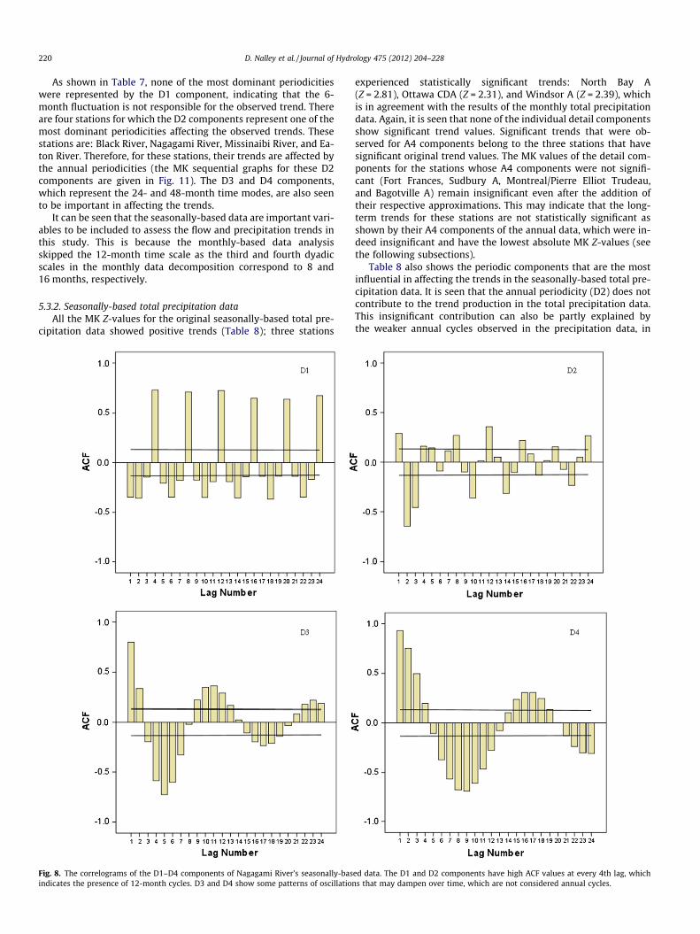
220 D. Nalley et al. / Journal of Hydrology 475 (2012) 204–228
As shown in Table 7, none of the most dominant periodicitieswere represented by the D1 component, indicating that the 6-month fluctuation is not responsible for the observed trend. Thereare four stations for which the D2 components represent one of themost dominant periodicities affecting the observed trends. Thesestations are: Black River, Nagagami River, Missinaibi River, and Ea-ton River. Therefore, for these stations, their trends are affected bythe annual periodicities (the MK sequential graphs for these D2components are given in Fig. 11). The D3 and D4 components,which represent the 24- and 48-month time modes, are also seento be important in affecting the trends.
It can be seen that the seasonally-based data are important vari-ables to be included to assess the flow and precipitation trends inthis study. This is because the monthly-based data analysisskipped the 12-month time scale as the third and fourth dyadicscales in the monthly data decomposition correspond to 8 and16 months, respectively.
5.3.2. Seasonally-based total precipitation dataAll the MK Z-values for the original seasonally-based total pre-
cipitation data showed positive trends (Table 8); three stations
Fig. 8. The correlograms of the D1–D4 components of Nagagami River’s seasonally-basindicates the presence of 12-month cycles. D3 and D4 show some patterns of oscillation
experienced statistically significant trends: North Bay A(Z = 2.81), Ottawa CDA (Z = 2.31), and Windsor A (Z = 2.39), whichis in agreement with the results of the monthly total precipitationdata. Again, it is seen that none of the individual detail componentsshow significant trend values. Significant trends that were ob-served for A4 components belong to the three stations that havesignificant original trend values. The MK values of the detail com-ponents for the stations whose A4 components were not signifi-cant (Fort Frances, Sudbury A, Montreal/Pierre Elliot Trudeau,and Bagotville A) remain insignificant even after the addition oftheir respective approximations. This may indicate that the long-term trends for these stations are not statistically significant asshown by their A4 components of the annual data, which were in-deed insignificant and have the lowest absolute MK Z-values (seethe following subsections).
Table 8 also shows the periodic components that are the mostinfluential in affecting the trends in the seasonally-based total pre-cipitation data. It is seen that the annual periodicity (D2) does notcontribute to the trend production in the total precipitation data.This insignificant contribution can also be partly explained bythe weaker annual cycles observed in the precipitation data, in
ed data. The D1 and D2 components have high ACF values at every 4th lag, whichs that may dampen over time, which are not considered annual cycles.

North Magnetawan River
Black River
Fort Frances A Bagotville A
Fig. 9. The correlograms of several approximation components (A4) of the seasonally-based data showing a lack of constant oscillations.
Table 7Mann–Kendall values of the seasonally-based flow series: original data, details components (D1–D4), approximations (A4), and a set of combination of the details and theirrespective approximations. The most dominant periodic components for trend are indicated in bold format.
Data Neebing River N. Magnetawan River Black River Sydenham River Nagagami River Missinaibi River Eaton River Richelieu River
Original �0.27 1.43 1.36 3.13* 1.31 �1.78 �0.22 3.06*
D1 �0.43 �0.20 0.89 �0.85 0.60 �0.43 �0.06 �0.45D2 �0.05 0.44 �0.46 0.61 �0.07 0.14 0.01 0.00D3 0.21 �0.59 0.16 �0.29 0.01 0.18 0.05 0.05D4 0.10 0.52 0.38 �0.27 0.00 0.14 �0.11 �0.04A4 �1.10 1.43 1.24 2.99* 1.53 �3.59* �0.77 3.52*
D1 + A4 �0.82 2.36* 0.91 3.75* 1.76 �3.19* �0.72 3.70*
D2 + A4 �0.99 2.09* 1.52 3.73* 1.14 �2.32⁄ �0.53 3.76*
D3 + A4 �0.45 1.64 0.92 2.54* 1.80 �2.48⁄ �0.54 2.97⁄
D4 + A4 �1.05 1.83 0.81 3.47⁄ 1.36 �2.81* �1.17 3.51⁄
* Indicates significant trend values at a = 5%.
D. Nalley et al. / Journal of Hydrology 475 (2012) 204–228 221
comparison to the flow data. Most of the precipitation trends areaffected by the D3 and D4 components, except for station NorthBay A, where D1 is considered the most dominant periodic compo-nent. We can suggest that the periodic components that mainly af-fect trends in the seasonally-based total precipitation are the 24- to48-month time scales (2–4 years). An example of the sequentialMK graphs for the different periodic components portraying their
trend lines with respect to their original data is given in Fig. 12(station used: Ottawa CDA).
5.4. Annual data analysis
The trend analysis of the monthly and seasonally-based datasuggests that there is a possibility of longer time-periodicity than

222 D. Nalley et al. / Journal of Hydrology 475 (2012) 204–228
just 48 and 64 months (which are the last periodic modes in theseasonally-based and monthly data decompositions, respectively).Many of the trends in the monthly and seasonally-based data areinfluenced by the higher time periodic components (i.e. lower-fre-quency events). The argument that there may be higher time peri-odicities affecting the trend in streamflow and precipitation is alsoreflected in the approximation components of the DWTs, whichshould carry the trend element (slowest-changing events) of thetime series: (1) many approximation components in the data anal-ysis showed significant MK Z-values; and (2) higher MK Z-values ofthe detail components were observed after the addition of theirrespective approximations. Annual time series were then analyzedin order to obtain a more thorough trend analysis. Each annualtime series was decomposed into four levels, which correspondto the 2-year, 4-year, 8-year and 16-year variations.
Although there is a mixture of positive and negative trends inthe annual flow, most of the stations exhibit positive trends. Threestreamflow stations have experienced significant trend: SydenhamRiver (Z = 2.37), Missinaibi River (Z = �2.23), and Richelieu River(Z = 2.92) (Table 9). Indeed, most studies focusing on streamflowtrends in Canada have generally found that the flow trends inCanadian rivers are not uniform. There are areas that experiencepositive trends while others are experiencing negative trends(due to factors such as temperature, amount of precipitation, andevapotranspiration).
For the annual total precipitation, only stations North Bay A(Z = +3.57) and Ottawa CDA (Z = +2.50) experienced significanttrend values (Table 10). It is worth mentioning that all of the origi-nal annual precipitation data (as well as most of the monthly andseasonally-based precipitation data) show positive trend values –
1960 1965 1970 1975 1980 1985 1990 1995 2000 2005-6
-4
-2
0
2
4
6
Z Va
lue
Year
1960 1965 1970 1975 1980 1985 1990 1995 2000 2005-6
-4
-2
0
2
4
6
Z Va
lue
Year
D1+A4
D3+A4
Fig. 10. Illustration of the sequential Mann–Kendall graphs of the D1–D4 componentsdominant periodic component for trend (Sydenham River’s data were used in this examsolid and dashed progressive lines are the original and detail component sequential MK
this prevalent increase in trends in the total precipitation seen inthis study are in agreement with findings from several other pre-cipitation studies. For example: Mekis and Hogg (1999) found thattotal annual precipitation in many parts of Canada is on the rise;Stone et al. (2000) reported that total annual precipitation in thesouth of Canada experienced an increase (from 1895 to 1996);Zhang et al. (2000) found that the total annual precipitation has in-creased across Canada by 5%-35%. Groleau et al. (2007) also foundthat 30% of the weather stations in southern Quebec and NewBrunswick, Canada, experienced significant positive trends duringwinter rainfall.
The periodic component(s) considered the most influential inaffecting trends in flow and precipitation data are indicated in Ta-bles 9 and 10, respectively. Examples of determining the mostdominant periodic components that affect the production of trendsin annual flow and precipitation series are given in Figs. 13 and 14,respectively. There are a few individual detail components (with-out approximation) that showed significant trend values (Tables9 and 10). However, these components do not end up being consid-ered the most influential time periodicities to affect the trends. Forexample, in Table 9, the MK Z-value of the D4 component of BlackRiver station is 2.38, but it is not found to be the most dominantperiodic component for trend. It is also seen that the differencein MK Z-value between the D4 (with approximation) and the origi-nal data is high. It is therefore not expected that the D4 detail com-ponent in Black River station would be the most influentialcomponent to affect the trend. This illustrates that when analyzingtrends in a dataset via the wavelet transform, not only should thefinal MK value for the different components be considered, but alsotheir sequential MK values in comparison to the original data.
1960 1965 1970 1975 1980 1985 1990 1995 2000 2005-6
-4
-2
0
2
4
6
Z Va
lue
Year
1960 1965 1970 1975 1980 1985 1990 1995 2000 2005-6
-4
-2
0
2
4
6
Z Va
lue
Year
D2+A4
D4+A4
(with approximation) of the seasonally-based data in order to determine the mostple). The upper and lower dashed lines represent the confidence limits (a = 5%); the
lines, respectively.

D. Nalley et al. / Journal of Hydrology 475 (2012) 204–228 223
Tables 9 and 10 show that the dominant periodic componentsplaying major roles in affecting the trends in the annual data arenot uniform. The most common dominant periodicities are D1and D2 (both with approximations added). This is an indicationthat the trends in the annual data over the study area are mainlycharacterized by 2- to 4-year periodic events (inter-annualfluctuations).
The progressive MK graphs of the annual data give indicationsthat most of the trends – positive or negative – visibly started dur-ing the period from 1965 to early 1970s (Figs. 15 and 16). This tim-ing is important as it has been noticed in several Canadian studiesthat 1970 serves as a point of change in streamflow and precipita-
1960 1965 1970 1975 1980 1985 1990 1995 2000 2005-6
-4
-2
0
2
4
6
Z Va
lue
Year
1960 1965 1970 1975 1980 1985 1990 1995 2000 2005-6
-4
-2
0
2
4
6
Z Va
lue
Year
Black River
Missinaibi River
Fig. 11. Sequential Mann–Kendall graphs of the D2 components, which represent the 12lines show good matches with respect their original trend lines. The upper and lower daslines are the original and detail component sequential MK lines, respectively.
Table 8Mann–Kendall values of the seasonally-based precipitation series: original data, details cotheir respective approximation. The most dominant periodic components for trends are in
Data Fort Frances A Sudbury A North Bay A Ottawa C
Original 0.72 1.32 2.81* 2.31*
D1 0.29 �0.66 �0.51 0.47D2 0.00 0.04 �0.23 �0.45D3 0.15 0.16 �0.02 0.41D4 0.59 0.00 0.93 0.22A4 0.81 1.76 5.09* 2.31*
D1 + A4 1.45 1.55 3.39⁄ 2.94*
D2 + A4 0.21 1.53 4.13* 2.17*
D3 + A4 0.64 1.55 4.01* 2.35⁄
D4 + A4 1.12 1.17 4.12* 2.59⁄
* Indicates significant trend values at a = 5%.
tion activities in relation to the atmospheric variability affectingCanadian climate, such as the Pacific/North America teleconnec-tion (PNA) and the North Atlantic Oscillation (NAO). Indeed, theseperiodic modes may also be associated with the North AtlanticOscillation (NAO), which has one of its main peaks centered at2 years (Cook et al., 1998; Anctil and Coulibaly, 2004). Fu et al.(2012), who studied the influence of solar activities and El Niñoon streamflow in southern Canada, indicated that there is a corre-lation between streamflow activities and solar activities at 11 and22 years. The correlation between streamflow activities in south-ern Canada and the El Niño cycles is at the 2–7 year periodicities(Fu et al., 2012). The combined effect of solar activities and El
1960 1965 1970 1975 1980 1985 1990 1995 2000 2005-6
-4
-2
0
2
4
6
Z Va
lue
Year
1960 1965 1970 1975 1980 1985 1990 1995 2000 2005-6
-4
-2
0
2
4
6
Z Va
lue
Year
Nagagami River
Eaton River
-month periodic components from several seasonally-based flow data. These trendhed lines represent the confidence limits (a = 5%); the solid and dashed progressive
mponents (D1–D4), approximations (A4), and a set of combination of the details anddicated in bold format.
DA Windsor A Montreal/Pierre Elliot Trudeau Bagotville A
2.39* 0.15 0.77�0.11 �1.70 �0.96
0.31 0.43 0.22�0.41 �0.25 0.06�0.20 �0.19 0.21
2.41* 0.19 0.622.09* �0.17 0.642.23* 0.03 0.631.21 �0.40 0.332.36⁄ 0.02 0.72

Table 9Mann–Kendall values of the annual flow series: original data, details components (D1–D4), approximations (A4), and a set of combination of the details and their respectiveapproximation. The most influential periodic components for trends are indicated in bold format.
Data Neebing River N. Magnetawan River Black River Sydenham River Nagagami River Missinaibi River Eaton River Richelieu River
Original �0.50 0.91 0.73 2.37* 1.12 �2.23* �0.46 2.92*
D1 �0.13 0.00 �0.19 �0.01 0.15 �0.16 0.22 0.19D2 �0.04 0.30 0.10 �0.15 0.17 �0.15 0.27 0.12D3 0.57 �0.13 0.06 0.51 0.25 �0.30 �0.28 0.46D4 �1.63 3.66* 2.38* 2.15* 1.22 �0.41 �0.55 0.15A4 �0.48 1.80 1.15 2.66* 1.96* �2.12* �0.79 3.09*
D1 + A4 �0.57 1.39 0.55 1.42 0.49 �1.73 �0.60 2.61*
D2 + A4 �0.73 1.55 0.68 1.47 0.96 �2.12⁄ �0.87 2.98*
D3 + A4 �0.19 0.94 0.80 2.51⁄ 0.94 �2.47* �0.97 1.99*
D4 + A4 �3.03* 3.95* 4.33* 3.17* 3.44* �4.57* �1.16 3.09⁄
* Indicates significant trend values at a = 5%.
1960 1965 1970 1975 1980 1985 1990 1995 2000 2005-6
-4
-2
0
2
4
6
Z Va
lue
Year1960 1965 1970 1975 1980 1985 1990 1995 2000 2005
-6
-4
-2
0
2
4
6
Z Va
lue
Year
-6
-4
-2
0
2
4
6
Z Va
lue
-6
-4
-2
0
2
4
6
Z Va
lue
D1+A4 D2+A4
D3+A4 D4+A4
1960 1965 1970 1975 1980 1985 1990 1995 2000 2005Year
1960 1965 1970 1975 1980 1985 1990 1995 2000 2005Year
Fig. 12. Sequential Mann–Kendall graphs of the components of the seasonally-based precipitation data from Ottawa CDA station. The upper and lower dashed lines representthe confidence limits (a = 5%); the solid and dashed progressive lines are the original and detail sequential MK lines, respectively. Based on the MK values and the sequentialMK graphs, D3 and D4 (with approximations) were determined to be the most effective periodic components contributing to the trend production.
Table 10Mann–Kendall values of the annual precipitation series: original data, details components (D1–D4), approximations (A4), and a set of combination of the details and theirrespective approximation. The most influential periodic components for trends are indicated in bold format.
Data Fort Frances A Sudbury A North Bay A Ottawa CDA Windsor A Montreal/Pierre Elliot Trudeau Bagotville A
Original 0.68 1.24 3.57* 2.50* 1.70 0.33 0.95D1 0.54 �0.16 �0.13 �0.41 0.04 0.06 �0.33D2 0.12 �0.28 0.39 0.19 0.33 0.25 �0.55D3 0.00 �0.18 0.70 0.49 0.96 0.58 0.99D4 1.32 2.51* 1.87 3.21* 2.31* �0.70 1.09A4 1.22 1.45 4.91* 2.45* 2.15* �0.02 1.28D1 + A4 0.68 1.34 2.35* 0.00 1.05 �0.31 �0.29D2 + A4 1.06 1.39 3.51⁄ 0.51 1.93 0.00 �0.12D3 + A4 0.65 2.45* 4.27* 1.84 3.27* 0.25 0.90D4 + A4 2.89* 3.82* 5.31* 3.14* 5.26* �0.91 1.63
* Indicates significant trend values at a = 5%.
224 D. Nalley et al. / Journal of Hydrology 475 (2012) 204–228

1960 1965 1970 1975 1980 1985 1990 1995 2000 2005-6
-4
-2
0
2
4
6
Z Va
lue
Year
-6
-4
-2
0
2
4
6
Z Va
lue
-6
-4
-2
0
2
4
6
Z Va
lue
-6
-4
-2
0
2
4
6
Z Va
lue
D1+A4 D2+A4
D3+A4 D4+A4
1960 1965 1970 1975 1980 1985 1990 1995 2000 2005Year
1960 1965 1970 1975 1980 1985 1990 1995 2000 2005Year
1960 1965 1970 1975 1980 1985 1990 1995 2000 2005Year
Fig. 13. Examples of sequential Mann–Kendall graphs of the detail components of the annual flow data in order to determine the most dominant periodicity for trends(Sydenham River’s data were used in this example). The upper and lower dashed lines represent the confidence limits (a = 5%); the solid and dashed progressive lines are theoriginal and detail sequential MK lines, respectively.
D. Nalley et al. / Journal of Hydrology 475 (2012) 204–228 225
Niño is found at 18–32 years (Fu et al., 2012). Here, as can be ob-served in Table 9, the most common dominant periodicities are2–4 years, which could also be related to the El Niño effect. TheRichelieu River’s most dominant periodicity is the 16-year mode,which may be a result of the combined effect of solar activitiesand the El Niño cycle. Prokoph et al. (2012) also found that themaximum annual streamflow activities in southern Canada havestrong 11-year cycles, which match the 11-year solar radiationactivities. It is also suggested that the effects of ENSO and NAOon precipitation, which in turn affect the streamflow activities insouthern Canada, are also evident (Prokoph et al., 2012). It is verylikely that multiple factors are affecting the precipitation andstreamflow trends over the study area.
In Fig. 15 it is observed that at six out of the eight flow stations,there were upward trends that started between 1965 and 1970. Infour out of these six stations, the trends stopped between 1980 and1985, followed by either downward trends or no trends. Fig. 16shows that positive trends started around 1965 at five out of theseven meteorological stations. Anctil and Coulibaly (2004), whoanalyzed the inter-annual variability of Quebec streamflow, alsoplaced an importance on the year 1970 because there was a posi-tive correlation between the streamflow activity (especially at the2–3 year band) and the PNA index since around 1970. Similarly,Coulibaly and Burn (2004), who analyzed annual Canadian stream-flow, also found 1970 as the change point in flow activity. Theyfound that the PNA and the NAO are the main dominant telecon-nection patterns for the period of 1950–1999 and after 1970,respectively (Coulibaly and Burn, 2004). Stone et al. (2000) studiedthe variability in Canadian precipitation and its intensity and re-lated them to the PNA and NAO. Different seasons and regions re-
sponded differently to the atmospheric variation, but both the NAOand the PNA were found to have a statistical significance in affect-ing precipitation intensity over Canada. For example, the NAO (po-sitive phase) has a significant impact, which affected theprecipitation intensity during a few 3-month seasons in easternCanada (Stone et al., 2000). The NAO has been in a positive phasesince around 1970 (Anctil and Coulibaly, 2004). The PNA also sig-nificantly affected the precipitation increase during autumn andwinter seasons in Ontario and southern Quebec, during the secondhalf of the 20th century (Stone et al., 2000). Therefore, the trendsobserved in this study, both in flow and precipitation data, couldbe related to the activity of these influential hydro-climatic indices.
6. Conclusions and recommendations
The DWT and the MK tests were applied on the mean flow andtotal precipitation datasets, over southern parts of Quebec and On-tario, in order to analyze their trends. The results of the trend anal-ysis showed that there are positive and negative trends; however,they were dominated mostly by positive trends. In order to deter-mine the most appropriate Daubechies (db) wavelet type and bor-der condition in the DWT procedure, not only were the MREsconsidered, but also the MK Z-value relative errors. This additionalcriterion proposed in this study was found to be very useful be-cause the differences in the er were much more noticeable com-pared to the differences in the MREs. In this study, the proposedrelative error criterion served as a better indicator in determiningthe number of decomposition levels, the mother wavelet, as wellas the extension border to be used in the data analysis – these is-

1960 1965 1970 1975 1980 1985 1990 1995 2000 2005-6
-4
-2
0
2
4
6Z
Valu
e
Year
-6
-4
-2
0
2
4
6
Z Va
lue
-6
-4
-2
0
2
4
6
Z Va
lue
-6
-4
-2
0
2
4
6
Z Va
lue
D1+A4 D2+A4
D3+A4 D4+A4
1960 1965 1970 1975 1980 1985 1990 1995 2000 2005Year
1960 1965 1970 1975 1980 1985 1990 1995 2000 2005Year
1960 1965 1970 1975 1980 1985 1990 1995 2000 2005Year
Fig. 14. Examples of sequential Mann–Kendall graphs of the detail components of the annual precipitation data in order to determine the most dominant periodicity fortrends (Ottawa CDA’s data were used in this example). The upper and lower dashed lines represent the confidence limits (a = 5%); the solid and dashed progressive lines arethe original and detail sequential MK lines, respectively.
Fig. 15. Progressive Mann–Kendall graphs of all the original annual flow data used in the study. The upper and lower dashed lines represent the confidence limits (a = 5%).These graphs were used to determine the possible starting time of the observed trends for the different stations.
226 D. Nalley et al. / Journal of Hydrology 475 (2012) 204–228
sues have not been addressed properly or in any detail in the exist-ing literature.
Although the periodic components that affect the trends are notall the same for all stations, a generalization can be made. For themonthly, seasonally-based, and annual flow data analysis, the mostcommon periodic components that were found to be the mosteffective in producing the observed trends are 8–32 months, 12–48 months (1–4 years), and 2–4 years, respectively. For themonthly, seasonally-based, and annual precipitation analysis, theperiodicities most commonly seen as the most important compo-nents are 32-months, 24–48 months (2–4 years), and 2–4 years,
respectively. This may be correlated to the NAO cycle becauseone of the main peaks of the NAO cycles is centered around2.1 years (Cook et al., 1998; Anctil and Coulibaly, 2004), whichseem to coincide with many of the main periodic components ofthe lower resolution data found in this study. As can be seen, thedifferent data types produced relatively similar conclusions interms of the most influential periodicities for trends. It may be con-cluded that for the mean flow and total precipitation over thestudy area, the trends are influenced by fluctuations of up to4 years. Although there is a total of 13 stations used in this study,similar conclusions were obtained – this could be attributed by the

Fig. 16. Progressive Mann–Kendall graphs of all the original precipitation data used in the study. The upper and lower dashed lines represent the confidence limits (a = 5%).These graphs were used to determine the possible starting time of the observed trends for the different stations.
D. Nalley et al. / Journal of Hydrology 475 (2012) 204–228 227
fact that the stations are located in relatively close proximity toeach other. Therefore, similar climatic factors are affecting the re-gions in which these stations are located.
The use of the DWT in this study clearly demonstrated howtime-scale information can be extracted from a dataset – this infor-mation can then be applied to studying how the trends observed inthe data were affected by certain time scales. Even for stations thatdid not exhibit significant trend values for their original data, thedecomposition of these data via the DWT was able to identifythe time scales that are considered important in affecting thetrends. This was accomplished by applying the MK trend tests onthe different time modes (detail components). With the sequentialMK tests, we were also able to identify the possible starting time inwhich the trend in a dataset started to appear. In the datasets usedin this study, an importance is placed at the time between 1965and 1970 because most of the trends appeared to start around thattime. Anctil and Coulibaly (2004) and Coulibaly and Burn (2004)showed the positive correlation between streamflow/precipitationactivities with the PNA cycles since 1970. In this study, most of theflow and precipitation trends started between 1965 and 1970. Fuet al. (2012) also indicated the existence of positive correlationsbetween streamflow in southern Canada and solar activities andEl Niño cycles. As can be seen, a number of long-term changes inclimate are also factors that may affect the streamflow and precip-itation trends over the study area – there is no single factor thatacts as the driver for the observed trends over the study area. Thisis reflected by the different large tele-connection patterns whosecycles seem to coincide with the dominant periodicities. Futurestudies could incorporate some quantitative linkages betweenthe most dominant periodicities that affect trends (both in flowand precipitation) and the climatic descriptor cycles (or how thecombined effects of these climatic descriptors influence thestreamflow and precipitation over the study area). This may poten-tially explain the time–frequency characteristics that affect thetrends in streamflow and precipitation over Quebec and Ontario.It would also be beneficial to include more stations from differenthydrographic regions within Ontario and Quebec, as well as inother Canadian provinces in order to compare the periodic compo-nents that affect the trends in these other areas. Additionally, theimplications of these time–frequency characteristics of trends onregional water resources can be looked at in more detail.
Finally, the results obtained from this present study presentedsome baseline information about the important periodicities thataffect the flow and precipitation trends over southern Ontarioand Quebec. This information can be integrated into the meth-ods/models aiming to investigate how natural fluctuations (e.g.changes in climate, fluctuations of climate indices, etc.) can affect
flow and precipitation trends over southern Ontario and Quebec.Furthermore, the analysis obtained from this study can serve asgrounds for basing the water resources design and planning withinthe watershed covered by the study area, as it involves making rea-sonable predictions or assumptions about future hydro-climaticconditions.
Acknowledgements
The authors of this paper would like to thank Dr. Eva Mekisfrom the Climate Research Division, Environment Canada for pro-viding the second generation adjusted precipitation datasets usedin this study. Funding provided by an NSERC Discovery Grant heldby Jan Adamowski is also acknowledged.
References
Abdul Aziz, O.I., Burn, D.H., 2006. Trends and variability in the hydrological regimeof the Mackenzie River Basin. J. Hydrol. 319 (1–4), 282–294.
Adamowski, K., Bocci, C., 2001. Geostatistical regional trend detection in river flowdata. Hydrol. Process. 15 (18), 3331–3341.
Adamowski, K., Bougadis, J., 2003. Detection of trends in annual extreme rainfall.Hydrol. Process. 17 (18), 3547–3560.
Adamowski, K., Prokoph, A., Adamowski, J., 2009. Development of a new method ofwavelet aided trend detection and estimation. Hydrol. Process. 23 (18), 2686–2696.
Ampitiyawatta, A.D., Guo, S., 2009. Precipitation trends in the Kalu Ganga basin inSri Lanka. J. Agric. Sci. 4 (1), 10–18.
Anctil, F., Coulibaly, P., 2004. Wavelet analysis of the interannual variability insouthern Québec streamflow. J. Clim. 17 (1), 163–173.
Assani, A.A., Charron, S., Matteau, M., Mesfioui, M., Quessy, J.-F., 2010. Temporalvariability modes of floods for catchments in the St. Lawrence watershed(Quebec, Canada). J. Hydrol. 385 (1–4), 292–299.
Birsan, M.-V., Molnar, P., Burlando, P., Pfaundler, M., 2005. Streamflow trends inSwitzerland. J. Hydrol. 314 (1–4), 312–329.
Boyer, C., Chaumont, D., Chartier, I., Roy, A.G., 2010. Impact of climate change on thehydrology of St. Lawrence tributaries. J. Hydrol. 384 (1–2), 65–83.
Bruce, L.M., Koger, C.H., Jiang, L., 2002. Dimensionality reduction of hyperspectraldata using discrete wavelet transform feature extraction. IEEE Trans. Geosci.Remote Sens. 40 (10), 2331–2338.
Burn, D.H., Hag Elnur, M.A., 2002. Detection of hydrologic trends and variability. J.Hydrol. 255 (1–4), 107–122.
Burn, D.H., Sharif, M., Zhang, K., 2010. Detection of trends in hydrological extremesfor Canadian watersheds. Hydrol. Process. 24 (13), 1781–1790.
Cannas, B., Fanni, A., See, L., Sias, G., 2006. Data preprocessing for river flowforecasting using neural networks: wavelet transforms and data partitioning.Phys. Chem. Earth 31 (18), 1164–1171.
Choi, T.-M., Yu, Y., Au, K.-F., 2011. A hybrid SARIMA wavelet transform method forsales forecasting. Decis. Support Syst. 51 (1), 130–140.
Chou, C.-M., 2007. Applying multi-resolution analysis to differential hydrologicalgrey models with dual series. J. Hydrol. 332 (1–2), 174–186.
Chou, C.-M., 2011. Wavelet-based multi-scale entropy analysis of complex rainfalltime series. Entropy 13 (1), 241–253.
Clark, J.S., Yiridoe, E.K., Burns, N.D., Astatkie, T., 2000. Regional climate change:trend analysis of temperature and precipitation series at selected Canadiansites. Can. J. Agric. Econ. 48 (1), 27–38.

228 D. Nalley et al. / Journal of Hydrology 475 (2012) 204–228
Coats, R., 2010. Climate change in the Tahoe basin: regional trends, impacts anddrivers. Climatic Change 102 (3), 435–466.
Cook, E.R., D’Arrigo, R.D., Briffa, K.F., 1998. A reconstruction of the North AtlanticOscillation using tree-ring chronologies from North America and Europe.Holocene 8, 1–9.
Coulibaly, P., Burn, D.H., 2004. Wavelet analysis of variability in annual Canadianstreamflows. Water Resour. Res. 40 (3), W03105.
Cunderlik, J.M., Burn, D.H., 2004. Linkages between regional trends in monthlymaximum flows and selected climatic variables. J. Hydrol. Eng. 9 (4), 246–256.
Daubechies, I., 1990. The wavelet transform, time-frequency localization and signalanalysis. IEEE Trans. Inf. Theory 36 (5), 961–1005.
Daubechies, I., 1992. Ten Lectures on Wavelets. SIAM, Philadelphia.de Artigas, M.Z., Elias, A.G., de Campra, P.F., 2006. Discrete wavelet analysis to assess
long-term trends in geomagnetic activity. Phys. Chem. Earth 31 (1–3), 77–80.Dietz, E.J., Killeen, T.J., 1981. A nonparametric multivariate test for monotone trend
with pharmaceutical applications. J. Am. Stat. Assoc. 76 (373), 169–174.Dong, X., Nyren, P., Patton, B., Nyren, A., Richardson, J., Maresca, T., 2008. Wavelets
for agriculture and biology: a tutorial with applications and outlook. Bioscience58 (5), 445–453.
Drago, A.F., Boxall, S.R., 2002. Use of the wavelet transform on hydro-meteorologicaldata. Phys. Chem. Earth 27 (32–34), 1387–1399.
Durdu, Ö.F., 2010. Effects of climate change on water resources of the BüyükMenderes River basin, western Turkey. Turk. J. Agric. Forest. 34 (4), 319–332.
Ehsanzadeh, E., Adamowski, K., 2007. Detection of trends in low flows acrossCanada. Can. Water Resour. J. 32 (4), 251–264.
Ehsanzadeh, E., Ouarda, T.B.M.J., Saley, H.M., 2011. A simultaneous analysis ofgradual and abrupt changes in Canadian low streamflows. Hydrol. Process. 25(5), 727–739.
Fu, C., James, A.L., Wachowiak, M.P., 2012. Analyzing the combined influence ofsolar activity and El Niño on streamflow across southern Canada. Water Resour.Res. 48 (5), W05507.
Fugal, D.L., 2009. Conceptual Wavelets in Digital Signal Processing: An In-depth,Practical Approach for the Non-mathematician, first ed. Space & SignalsTechnologies LLC.
Goodwin, D.A., 2008. Wavelet Analysis of Temporal Data. Dissertation, Departmentof Statistics, The University of Leeds, Leeds, UK.
Groleau, A., Mailhot, A., Talbot, G., 2007. Trend analysis of winter rainfall oversouthern Québec and New Brunswick (Canada). Atmos. Ocean 45 (3), 153–162.
Hamed, K.H., 2008. Trend detection in hydrologic data: the Mann–Kendall trend testunder the scaling hypothesis. J. Hydrol. 349 (3–4), 350–363.
Hamed, K.H., Rao, A.R., 1998. A modified Mann–Kendall trend test forautocorrelated data. J. Hydrol. 204 (1–4), 182–196.
Hirsch, R.M., Slack, J.R., 1984. A nonparametric trend test for seasonal data withserial dependence. Water Resour. Res. 20 (6), 727–732.
Hirsch, R.M., Slack, J.R., Smith, R.A., 1982. Techniques of trend analysis for monthlywater quality data. Water Resour. Res. 18 (1), 107–121.
IPCC, 2007. Climate change 2007: the fourth IPCC scientific assessment. In: Parry,M.L., Canziani, O.F., Palutikof, J.P., van der Linden, P.J., Hanson, C.E. (Eds.),Intergovernmental Panel on Climate Change. Cambridge University Press,Cambridge, United Kingdom and New York, NY, USA.
Kallache, M., Rust, H.W., Kropp, J., 2005. Trend assessment: applications forhydrology and climate research. Nonlinear Process. Geophys. 12 (2), 201–210.
Kendall, M.G., 1975. Rank Correlation Methods. Griffin, London, UK.Kim, S., 2004. Wavelet analysis of precipitation variability in northern California,
USA. KSCE J. Civ. Eng. 8 (4), 471–477.Kisi, O., Cimen, M., 2011. A wavelet-support vector machine conjunction model for
monthly streamflow forecasting. J. Hydrol. 399 (1–2), 132–140.Kulkarni, J.R., 2000. Wavelet analysis of the association between the Southern
Oscillation and the Indian summer monsoon. Int. J. Climatol. 20 (1), 89–104.Kumar, S., Merwade, V., Kam, J., Thurner, K., 2009. Streamflow trends in Indiana:
effects of long term persistence, precipitation and subsurface drains. J. Hydrol.374 (1–2), 171–183.
Labat, D., 2005. Recent advances in wavelet analyses: Part 1. A review of concepts. J.Hydrol. 314 (1–4), 275–288.
Labat, D., Goddéris, Y., Probst, J.L., Guyot, J.L., 2004. Evidence for global runoffincrease related to climate warming. Adv. Water Resour. 27 (6), 631–642.
Liu, D., Chen, X., Lian, Y., Lou, Z., 2010. Impacts of climate change and humanactivities on surface runoff in the Dongjiang River basin of China. Hydrol.Process. 24 (11), 1487–1495.
Mallat, S.G., 1989. A theory for multiresolution signal decomposition: the waveletrepresentation. IEEE Trans. Pattern Anal. Mach. Intell. 11 (7), 674–693.
Mann, H.B., 1945. Nonparametric tests against trend. Econometrica 13 (3), 245–259.
McBean, E., Motiee, H., 2006. Assessment of impacts of climate change on waterresources – a case study of the Great Lakes of North America. Hydrol. Earth Syst.Sci. Discuss. 3 (5), 3183–3209.
Mekis, E., Hogg, W.D., 1999. Rehabilitation and analysis of Canadian dailyprecipitation time series. Atmos. Ocean 37 (1), 53–85.
Mekis, É., Vincent, L.A., 2011. An overview of the second generation adjusted dailyprecipitation dataset for trend analysis in Canada. Atmos. Ocean 49 (2), 163–177.
Mishra, A.K., Singh, V.P., 2010. Changes in extreme precipitation in Texas. J.Geophys. Res. 115 (D14), D14106.
Mohsin, T., Gough, W., 2010. Trend analysis of long-term temperature time series inthe Greater Toronto Area (GTA). Theor. Appl. Climatol. 101 (3), 311–327.
Nolin, A.W., Hall-McKim, E.A., 2006. Frequency modes of monsoon precipitation inArizona and New Mexico. Mon. Weather Rev. 134 (12), 3774–3781.
Önöz, B., Bayazit, M., 2003. The power of statistical tests for trend detection. Turk. J.Eng. Environ. Sci. 27 (4), 247.
Partal, T., 2010. Wavelet transform-based analysis of periodicities and trends ofSakarya basin (Turkey) streamflow data. River Res. Appl. 26 (6), 695–711.
Partal, T., Küçük, M., 2006. Long-term trend analysis using discrete waveletcomponents of annual precipitations measurements in Marmara region(Turkey). Phys. Chem. Earth 31 (18), 1189–1200.
Percival, D.B., 2008. Analysis of geophysical time series using discrete wavelettransforms: an overview. In: Donner, R.V., Barbosa, S.M. (Eds.), Nonlinear TimeSeries Analysis in the Geosciences – Applications in Climatology, Geodynamics,and Solar-terrestrial Physics. Springer, Berlin/Heidelberg.
Popivanov, I., Miller, R.J., 2002. Similarity search over time-series data usingwavelets. In: Proceedings 18th International Conference on Data Engineering,pp. 212–221.
Popoola, A.O., 2007. Fuzzy-wavelet Method for Time Series Analysis. Dissertation,Department of Computing, School of Electronics and Physical Sciences,University of Surrey, Guildford, UK.
Prokoph, A., Adamowski, J., Adamowski, K., 2012. Influence of the 11 year solar cycleon annual streamflow maxima in Southern Canada. J. Hydrol. 442–443, 55–62.
Quiroz, R., Yarlequé, C., Posadas, A., Mares, V., Immerzeel, W.W., 2011. Improvingdaily rainfall estimation from NDVI using a wavelet transform. Environ. Modell.Softw. 26 (2), 201–209.
Roy, L., Leconte, R., Brissette, F.P., Marche, C., 2001. The impact of climate change onseasonal floods of a southern Quebec river basin. Hydrol. Process. 15 (16),3167–3179.
Santos, C.A.G., Galvão, C.d.O., Suzuki, K., Trigo, R.M., 2001. Matsuyama city rainfalldata analysis using wavelet transform. Annu. J. Hydraul. Eng., JSCE 45, 6.
Shao, Q., Li, Z., Xu, Z., 2010. Trend detection in hydrological time series by segmentregression with application to Shiyang River basin. Stoch. Env. Res. Risk Assess.24 (2), 221–233.
Stone, D.A., Weaver, A.J., Zwiers, F.W., 2000. Trends in Canadian precipitationintensity. Atmos. Ocean 38 (2), 321–347.
Su, H., Liu, Q., Li, J., 2011. Alleviating border effects in wavelet transforms fornonlinear time-varying signal analysis. Adv. Electr. Comput. Eng. 11 (3), 6.
Svensson, C., Kundzewicz, W.Z., Maurer, T., 2005. Trend detection in river flowseries: 2. Flood and low-flow index series. Hydrol. Sci. J. 50 (5), 824.
Timofeev, A., Sterin, A., 2010. Using the quantile regression method to analyzechanges in climate characteristics. Russ. Meteorol. Hydrol. 35 (5), 310–319.
Torrence, C., Compo, G.P., 1998. A practical guide to wavelet analysis. Bull. Am.Meteorol. Soc. 79 (1), 61–78.
Vonesch, C., Blu, T., Unser, M., 2007. Generalized Daubechies wavelet families. IEEETrans. Signal Process. 55 (9), 4415–4429.
Wang, W., Hu, S., Li, Y., 2011. Wavelet transform method for synthetic generation ofdaily streamflow. Water Resour. Manage. 25 (1), 41–57.
Xu, J., Chen, Y., Li, W., Ji, M., Dong, S., Hong, Y., 2009. Wavelet analysis andnonparametric test for climate change in Tarim River basin of Xinjiang during1959–2006. Chin. Geogr. Sci. 19 (4), 306–313.
Yue, S., Pilon, P., 2004. A comparison of the power of the t-test, Mann–Kendall andbootstrap tests for trend detection. Hydrol. Sci. J. 49 (1), 21–37.
Yue, S., Pilon, P., 2005. Probability distribution type of Canadian annual minimumstreamflow. Hydrol. Sci. J. 50 (3), 438.
Yue, S., Pilon, P., Phinney, B., Cavadias, G., 2002. The influence of autocorrelation onthe ability to detect trend in hydrological series. Hydrol. Process. 16 (9), 1807–1829.
Zhang, X., Vincent, L.A., Hogg, W.D., Niitsoo, A., 2000. Temperature and precipitationtrends in Canada during the 20th century. Atmos. Ocean 38 (3), 395–429.
Zhang, X., Harvey, K.D., Hogg, W.D., Yuzyk, T.R., 2001. Trends in Canadianstreamflow. Water Resour. Res. 37 (4), 987–998.
Zhang, Q., Xu, C.Y., Zhang, Z., Chen, Y.D., Liu, C.L., 2009. Spatial and temporalvariability of precipitation over China, 1951–2005. Theor. Appl. Climatol. 95 (1–2), 53–68.
Zhang, Z., Dehoff, A., Pody, R., Balay, J., 2010. Detection of streamflow change in theSusquehanna River basin. Water Resour. Manage. 24 (10), 1947–1964.
Zume, J., Tarhule, A., 2006. Precipitation and streamflow variability in NorthwesternOklahoma, 1894–2003. Phys. Geogr. 27 (3), 189–205.