London School of Economics, U.K. - Duke...

INTERNATIONAL ECONOMIC REVIEWVol. 47, No. 2, May 2006

MODELLING ASYMMETRIC EXCHANGE RATE DEPENDENCE∗

BY ANDREW J. PATTON1

London School of Economics, U.K.

We test for asymmetry in a model of the dependence between the Deutsche

mark and the yen, in the sense that a different degree of correlation is exhibited

during joint appreciations against the U.S. dollar versus during joint deprecia-

tions. We consider an extension of the theory of copulas to allow for conditioning

variables, and employ it to construct flexible models of the conditional depen-

dence structure of these exchange rates. We find evidence that the mark–dollar

and yen–dollar exchange rates are more correlated when they are depreciating

against the dollar than when they are appreciating.

1. INTRODUCTION

Evidence that the univariate distributions of many common economic variablesare nonnormal has been widely reported, as far back as Mills (1927). Commonexamples of deviations from normality include excess kurtosis (or fat tails) andskewness in univariate distributions. Recent studies of equity returns have alsoreported deviations from multivariate normality, in the form of asymmetric de-pendence. One example of asymmetric dependence is where two returns exhibitgreater correlation during market downturns than market upturns, as reported inErb et al. (1994), Longin and Solnik (2001), and Ang and Chen (2002). Variousexplanations for the presence of asymmetric dependence between equity returnshave been proffered. For example, Ribeiro and Veronesi (2002) suggest corre-lations between international stock markets increase during market downturnsas a consequence of investors having greater uncertainty about the state of theeconomy.

Much less attention has been paid to the possibility of asymmetric dependencebetween exchange rates. Asymmetric responses of central banks to exchange ratemovements is a possible cause of asymmetric dependence. For example, a desire

∗ Manuscript received June 2003; revised January 2005.1 This article is based on Chapter I of my Ph.D. dissertation, Patton (2002), and was previously cir-

culated under the title “Modelling Time-Varying Exchange Rate Dependence Using the Conditional

Copula.” I would like to thank Graham Elliott, Rob Engle, Raffaella Giacomini, Tony Hall, Joshua

Rosenberg, Kevin Sheppard, Allan Timmermann, four anonymous referees, and seminar participants

at the Econometric Society meetings in Maryland, Board of Governors of the Federal Reserve, Chicago

Graduate School of Business, Commonwealth Scientific and Industrial Research Organisation,

London School of Economics, Michigan State, Monash, Oxford, Pennsylvania, Princeton, Purdue,

Texas A&M, UCSD, UC-Riverside, University of Technology Sydney, and Yale for their comments

and suggestions. Financial support from the UCSD Project in Econometric Analysis Fellowship is

gratefully acknowledged. Please address correspondence to: A. J. Patton, Financial Markets Group,

London School of Economics, Houghton Street, London WC2A 2AE, U.K. E-mail: [email protected].

527

528 PATTON

to maintain the competitiveness of Japanese exports to the United States. withGerman exports to the United States. would lead the Bank of Japan to interveneto ensure a matching depreciation of the yen against the dollar whenever theDeutsche mark (DM) depreciated against the U.S. dollar. Such a scenario wasconsidered by Takagi (1999). On the other hand, a preference for price stabilitycould lead the Bank of Japan to intervene to ensure a matching appreciation of theyen against the dollar whenever the DM appreciated against the U.S. dollar. Animbalance in these two objectives could cause asymmetric dependence betweenthese exchange rates. If the competitiveness preference dominates the price sta-bility preference, we would expect the DM and yen to be more dependent duringdepreciations against the dollar than during appreciations. An alternative causecould come from portfolio rebalancing: When the dollar strengthens there is of-ten a shift of funds from other currencies into the dollar, whereas when the dollarweakens much of these funds shift into the DM or euro instead of the yen, as theformer was/is the second most important currency.2 Such rebalancing behaviorwould also lead to greater dependence during depreciations of the DM and yenagainst the dollar than during appreciations.

To investigate whether the dependence structure of these exchange rates isasymmetric, we make use of a theorem due to Sklar (1959), which shows that anyn-dimensional joint distribution function may be decomposed into its n marginaldistributions, and a copula, which completely describes the dependence betweenthe n variables.3 The copula is a more informative measure of dependence betweentwo (or more) variables than linear correlation, as when the joint distribution ofthe variables of interest is nonelliptical the usual correlation coefficient is no longersufficient to describe the dependence structure.

By using an extension of Sklar’s theorem, we are able to exploit the success wehave had in the modeling of univariate densities by first specifying models for themarginal distributions of a multivariate distribution of interest, and then specify-ing a copula. For example, consider the modeling of the joint distribution of twoexchange rates: The Student’s t distribution has been found to provide a reason-able fit to the conditional univariate distribution of daily exchange rate returns;see Bollerslev (1987) among others. A natural starting point in the modeling of thejoint distribution of two exchange rates might then be a bivariate t distribution.However, the standard bivariate Student’s t distribution has the restrictive prop-erty that both marginal distributions have the same degrees of freedom parameter.Studies such as Bollerslev (1987) have shown that different exchange rates havedifferent degrees of freedom parameters, and our empirical results confirm thatthis is true for the Deutsche mark–U.S. dollar and yen–U.S. dollar exchange rates:The restriction that both exchange rate returns have the same degrees of freedom

2 I thank a referee for providing these further suggestions on possible sources of asymmetric ex-

change rate dependence.3 The word copula comes from Latin for a “link” or “bond,” and was coined by Sklar (1959), who

first proved the theorem that a collection of marginal distributions can be “coupled” together via

a copula to form a multivariate distribution. It has been given various names, such as dependencefunction (Galambos, 1978, and Deheuvels, 1978), uniform representation (Kimeldorf and Sampson,

1975, and Hutchinson and Lai, 1990), or standard form (Cook and Johnson, 1981).

MODELING ASYMMETRIC DEPENDENCE 529

parameter is rejected by the data. Note also that this is possibly the most idealsituation: where both assets turn out to have univariate distributions from thesame family, the Student’s t, and very similar degrees of freedom (6.2 for the markand 4.3 for the yen). We could imagine situations where the two variables of in-terest have quite different marginal distributions, where no obvious choice for thebivariate density exists. Further, the bivariate Student’s t distribution imposes asymmetric dependence structure, ruling out the possibility that the exchange ratesmay be more or less dependent during appreciations than during depreciations.Decomposing the multivariate distribution into the marginal distributions and thecopula allows for the construction of better models of the individual variables thanwould be possible if we constrained ourselves to look only at existing multivariatedistributions.

A useful parametric alternative to copula-based multivariate models is a multi-variate regime switching model; see Ang and Bekaert (2002) for example. Theseauthors show that a mixture of two multivariate normal distributions can matchthe asymmetric equity-return dependence found in Longin and Solnik (2001),and thus may also be useful for studying asymmetric exchange rate dependence.A detailed comparison of flexible copula-based models and flexible multivariateregime switching models for exchange rates and/or equity returns would be aninteresting study, but we leave it for future research.

An alternative to parametric specifications of the multivariate distributionwould, of course, be a nonparametric estimate, as in Fermanian and Scaillet (2003)for example, which can accommodate all possible distributional forms. One com-mon drawback with nonparametric approaches is the lack of precision that occurswhen the dimension of the distribution of interest is moderately large (say overfour), or when we consider multivariate distributions conditioned on a state vector(as is the case in this article). The trade-off for this lack of precision is the fact thata parametric specification may be misspecified. It is for this reason that we devotea great deal of attention to tests of goodness-of-fit of the proposed specifications.

This article makes two contributions. Our first contribution is to consider howthe theory of (unconditional) copulas may be extended to the conditional case,thus allowing us to use copula theory in the analysis of time-varying conditionaldependence. Time variation in the conditional first and second moments of eco-nomic time series has been widely reported, and so allowing for time variationin the conditional dependence between economic time series seems natural. Thesecond and main contribution of the article is to show how we may use con-ditional copulas for multivariate density modeling. We examine daily Deutschemark–U.S. dollar (DM–USD) and Japanese yen–U.S. dollar (Yen–USD) exchangerates over the period January 1991 to December 2001, and propose a new copulathat allows for asymmetric dependence and includes symmetric dependence as aspecial case. We find significant evidence that the dependence structure betweenthe DM–USD and Yen–USD exchange rates was asymmetric, consistent with theasymmetric central bank behavior story presented above. We also find very strongevidence of a structural break in the conditional copula following the introduc-tion of the euro in January 1999: The level of dependence drops substantially,the dynamics of conditional dependence change, and the dependence structure

530 PATTON

goes from significantly asymmetric in one direction to weakly asymmetric in theopposite direction.

The modeling of the entire conditional joint distribution of these exchangerates has a number of attractive features: Given the conditional joint distribution,we can, of course, obtain conditional means, variances, and correlation, as wellas the time paths of any other dependence measure of interest, such as rankcorrelation or tail dependence.4 Further, there are economic situations where theentire conditional joint density is required, such as the pricing of financial optionswith multiple underlying assets (see Rosenberg, 2003) or in the calculation ofportfolio Value-at-Risk (VaR) (see Hull and White, 1998) or in a forecast situationwhere the loss function of the forecast’s end user is unknown.

Despite the fact that copulas were introduced as a means of isolating the depen-dence structure of a multivariate distribution over 40 years ago, it is only recentlythat they attracted the attention of economists. In the last few years, numerouspapers have appeared, using copulas in such applications as multivariate optionpricing, asset allocation, models of default risk, integrated risk management, selec-tivity bias, nonlinear autoregressive dependence, and contagion.5 To our knowl-edge, this article is one of the first to consider copulas for time-varying condi-tional distributions, emphasize the importance of formal goodness-of-fit testingfor copulas and marginal distributions, and to employ statistical tests comparingthe goodness-of-fit of competing nonnested copulas.

The structure of the remainder of this article is as follows. In Section 2, wepresent the theory of the conditional copula. In Section 3, we apply the theory ofconditional copulas to a study of the dependence structure of the Deutsche mark–U.S. dollar and yen–U.S. dollar exchange rates. In that section, we discuss theconstruction and evaluation of time-varying conditional copula models. We sum-marize our results in Section 4. Details on the goodness-of-fit tests are presentedin the Appendix.

2. THE CONDITIONAL COPULA

In this section we review the theory of copulas and discuss the extension tohandle conditioning variables. Though in this article we focus on bivariate distri-butions, it should be noted that the theory of copulas is applicable to the moregeneral multivariate case. We must first define the notation: The variables of in-terest are X and Y and the conditioning variable is W, which may be a vector.Let the joint distribution of (X, Y, W) be FXYW , denote the conditional distribu-tion of (X, Y) given W, as FXY|W , and let the conditional marginal distributionsof X | W and Y | W be denoted FX|W and FY|W , respectively. Recall that

4 This measure will be discussed in more detail in Section 3. Dependence during extreme events

has been the subject of much analysis in the financial contagion literature; see Hartmann et al. (2004)

among others.5 See Frees et al. (1996), Bouye et al. (2000a, 2000b), Cherubini and Luciano (2001, 2002), Costinot

et al. (2000), Li (2000), Fermanian and Scaillet (2003), Embrechts et al. (2001), Granger et al. (forth-

coming), Frey and McNeil (2001), Rockinger and Jondeau (2001), Sancetta and Satchell (2001), Smith

(2003), Rodriguez (2003), Rosenberg (2003), Cherubini et al. (2004), Patton (2004a), Rosenberg and

Schuermann (2004), and Chen and Fan (2006).


F X|W(x|w) = FXY|W(x, ∞ | w) and FY|W(y | w) = FXY|W(∞, y | w). We will as-sume in this article that the distribution function FXYW is sufficiently smooth forall required derivatives to exist, and that FX|W , FY|W , and FXY|W are continuous.The latter assumptions are not necessary, but making them simplifies the presenta-tion. Throughout this article, we will denote the distribution (or c.d.f .) of a randomvariable using an uppercase letter, and the corresponding density (or p.d.f .) usingthe lowercase letter. We will denote the extended real line as R ≡ R ∪ {±∞}. Weadopt the usual convention of denoting random variables in upper case, Xt, andrealizations of random variables in lower case, xt.

A thorough review of (unconditional) copulas may be found in Nelsen (1999)and Joe (1997). Briefly, copula theory enables us to decompose a joint distributioninto its marginal distributions and its dependence function, or copula:

FXY(x, y) = C(FX(x), FY(y)), or(1)

fxy(x, y) = fx(x) · fy(y) · c(FX(x), FY(y))(2)

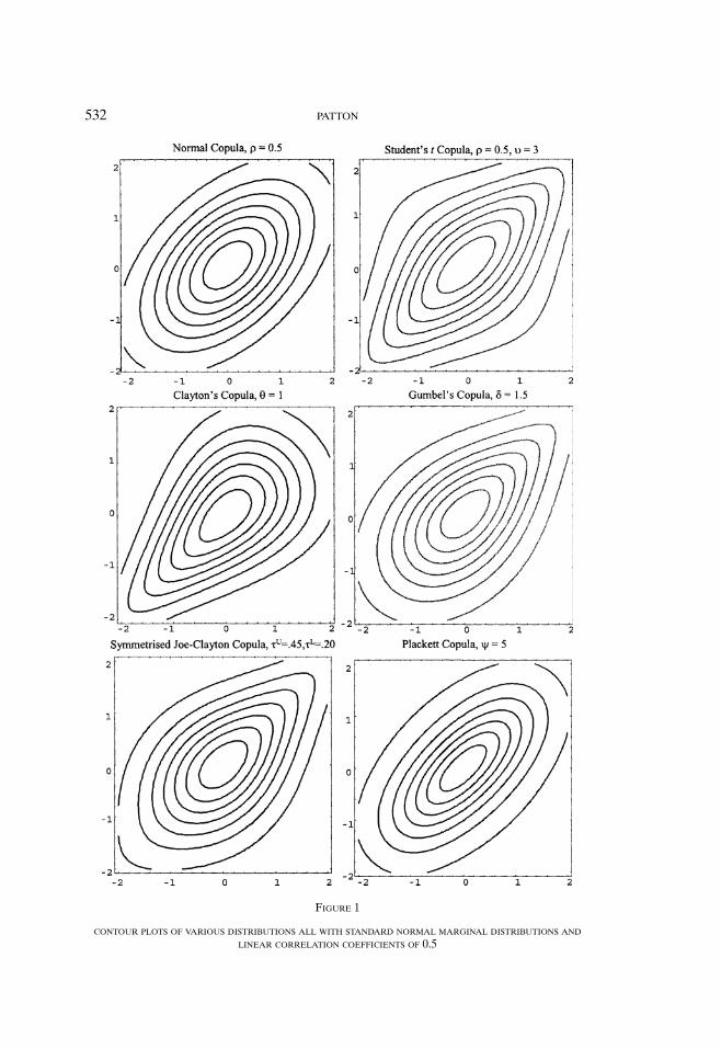
where Equation (1) above decomposes a bivariate cdf , and Equation (2) decom-poses a bivariate density. To provide some idea as to the flexibility that copulatheory gives us, we now consider various bivariate distributions, all with standardnormal marginal distributions and all implying a linear correlation coefficient, ρ,of 0.5. The contour plots of these distributions are presented in Figure 1. In theupper left corner of this figure is the standard bivariate normal distribution withρ = 0.5. The other elements of this figure show the dependence structures impliedby other copulas, with each copula calibrated so as to also yield ρ = 0.5. It is quiteclear that knowing the marginal distributions and linear correlation is not suffi-cient to describe a joint distribution: Clayton’s copula, for example, has contoursthat are quite peaked in the negative quadrant, implying greater dependence forjoint negative events than for joint positive events. Gumbel’s copula implies theopposite. The functional form of the symmetrized Joe–Clayton will be given inSection 3; the remaining copula functional forms may be found in Joe (1997) orPatton (2004).

Now let us focus on the modifications required for the extension to conditionaldistributions. Assume below that the dimension of the conditioning variable, W,is 1. Then the conditional bivariate distribution of (X, Y) | W can be derived fromthe unconditional joint distribution of (X, Y, W) as follows:

FXY|W(x, y | w) = fw(w)−1 · ∂ FXYW(x, y, w)

∂w, for w ∈ W

where f w is the unconditional density of W, and W is the support of W. However,the conditional copula of (X, Y) | W cannot be derived from the unconditionalcopula of (X, Y, W); further information is required.6 One definition of the con-ditional copula of (X, Y) | W is given below.

6 We thank a referee for pointing out that the conditional copula can be obtained given just the

unconditional copula of (X, Y, W) and the marginal density of W.

532 PATTON

FIGURE 1

CONTOUR PLOTS OF VARIOUS DISTRIBUTIONS ALL WITH STANDARD NORMAL MARGINAL DISTRIBUTIONS AND

LINEAR CORRELATION COEFFICIENTS OF 0.5


DEFINITION 1. The conditional copula of (X, Y) | W = w, where X | W =w ∼ F X|W(· | w) and Y | W = w ∼FY|W(· | w), is the conditional joint distributionfunction of U ≡ F X|W(X | w) and V ≡ FY|W(Y | w) given W = w.

The two variables U and V are known as the conditional “probability integraltransforms” of X and Y given W. Fisher (1932) and Rosenblatt (1952) showed thatthese random variables have the Unif (0, 1) distribution, regardless of the originaldistributions.7 It is simple to extend existing results to show that a conditionalcopula has the properties of an unconditional copula, for each w ∈ W ; see Patton(2002) for details. We now move on to an extension of Sklar’s (1959); theorem forconditional distributions:

THEOREM 1. Let F X|W(· | w) be the conditional distribution of X | W = w,FY|W(· | w) be the conditional distribution of Y | W = w, FXY|W(· | w) be the jointconditional distribution of (X, Y) | W = w, and W be the support of W. Assumethat F X|W(· | w) and FY|W(· | w) are continuous in x and y for all w ∈W . Then thereexists a unique conditional copula C(· | w) such that

FXY|W(x, y | w) = C(FX|W(x | w), FY|W(y | w) | w),

∀(x, y) ∈ R × R and each w ∈ W(3)

Conversely, if we let F X|W(· | w) be the conditional distribution of X | W = w,FY|W(· | w) be the conditional distribution of Y | W = w, and {C(· | w)} be a familyof conditional copulas that is measurable in w, then the function FXY|W(· | w) definedby Equation (3) is a conditional bivariate distribution function with conditionalmarginal distributions FX|W(· | w) and FY|W(· | w).

It is the converse of Sklar’s theorem that is the most interesting for multivariatedensity modeling. It implies that we may link together any two univariate distribu-tions, of any type (not necessarily from the same family), with any copula and wewill have defined a valid bivariate distribution. The usefulness of this result stemsfrom the fact that although in the economics and statistics literatures we have avast selection of flexible parametric univariate distributions, the set of parametricmultivariate distributions available is much smaller. With Sklar’s theorem, the setof possible parametric bivariate distributions is increased substantially, though, ofcourse, not all of these distributions will be useful empirically. With a corollaryto Sklar’s theorem, given in Nelsen (1999) for example, the set of possible para-metric multivariate distributions increases even further, as we are able to extractthe copula from any given multivariate distribution and use it independently ofthe marginal distributions of the original distribution. This corollary allows usto extract, for example, the “normal copula” from a standard bivariate normaldistribution.

7 The probability integral transform has also been used in the context of goodness-of-fit tests as far

back as the 1930s; see Pearson (1933) for example. More recently, Diebold et al. (1998) extended the

probability integral transform theory to the time series case, and proposed using it in the evaluation

of density forecasts.

534 PATTON

The only complication introduced when extending Sklar’s theorem to condi-tional distributions is that the conditioning variable(s), W, must be the same forboth marginal distributions and the copula. This is important in the construction ofconditional density models using copula theory. Failure to use the same condition-ing variable for F X|W, FY|W, and C will, in general, lead to a failure of the functionFXY|W to satisfy the conditions for it to be a joint conditional distribution function.For example, say we condition X on W1, Y on W2, and the copula on (W1, W2),and then specify F XY|W1,W2

(x, y | w1, w2) = C(FX|W1(x | w1), FY|W2

(y | w2)|w1, w2).Then F XY|W1,W2

(x, ∞ | w1, w2) = C(FX|W1(x | w1), 1 | w1, w2) = FX|W1

(x | w1), theconditional distribution of X | W1, which is the conditional marginal distribu-tion of (X, Y) | W1. But F XY|W1,W2

(∞, y | w1, w2) = C(1, FY | W2(y, |w2)|w1, w2) =

FY|W2(y, |w2), the conditional distribution of Y | W2, which is the conditional

marginal distribution of (X, Y) | W2. Thus the function F XY|W1,W2will not be the

joint distribution of (X, Y) | (W1, W2) in general.The only case when F XY|W1,W2

will be the joint distribution of (X, Y) | (W1,W2) is when FX|W1

(x | w1) = FX|W1,W2(x | w1, w2) for all (x, w1, w2) ∈ R × W1 × W2

and FY|W2(y, | w2) = FY|W1,W2

(y, | w1, w2) for all (y, w1, w2) ∈ R × W1 × W2. Al-though this is obviously a special case, it is not uncommon to find that certainvariables affect the conditional distribution of one variable but not the other, andthus this condition is satisfied. For example, in our empirical application we findthat, conditional on lags of the DM–USD exchange rate, lags of the Yen–USDexchange rate do not impact the distribution of the DM–USD exchange rate. Sim-ilarly, lags of the DM–USD exchange rate do not affect the Yen–USD exchangerate, conditional on lags of the Yen–USD exchange rate. Thus, in our case theabove condition is satisfied, though it must be tested in each separate application.

The density function equivalent of (3) is useful for maximum likelihood esti-mation, and is easily obtained provided that FX|Y and FY|W are differentiable andFXY|W and C are twice differentiable.

fXY|W(x, y | w) ≡ ∂2 FXY|W(x, y | w)

∂x∂y

= ∂ FX|W(x | w)

∂x· ∂ FY|W(y | w)

∂y· ∂2C(FX|W(x | w), FY|W(y | w) | w)

∂u∂v

fXY|W(x, y | w) ≡ fX|W(x | w) · fY|W(y | w) · c(u, v | w), ∀(x, y, w) ∈ R × R × W(4)

so LXY = LX + LY + LC(5)

where u ≡ F X|W(x | w), and v ≡ FY|W(y | w),LXY ≡ log fXY|W(x, y | w),LX ≡log fX|W(x | w),LY ≡ log fY|W(y | w), and LC ≡ log c(u, v | w).

3. THE CONDITIONAL DEPENDENCE BETWEEN THE MARK AND THE YEN

In this section we apply the theory of conditional copulas to the modeling ofthe conditional bivariate distribution of the daily Deutsche mark–U.S. dollar and


Japanese yen–U.S. dollar exchange rate returns over the period January 2, 1991,to December 31, 2001. This represents the post-unification era in Germany (Eastand West Germany were united in late 1989, and some financial integration wasstill being carried out during 1990) and includes the first 3 years of the euro’s reignas the official currency of Germany.8 The Yen–USD and DM–USD (euro–USDsince 1999) exchange rates are the two most heavily traded, representing close to50% of total foreign exchange trading volume.9 Given their status, the DM–USDand Yen–USD exchange rates have been relatively widely studied; see Andersenand Bollerslev (1998), Diebold et al. (1999), Andersen et al. (2001), among others.However, there has not, to our knowledge, been any investigation of the symmetryof the dependence structure between these exchange rates.

Table 1 presents some summary statistics of the data. The data were takenfrom the database of Datastream International and as usual we analyze the log-difference of each exchange rate. The table shows that neither exchange rate hada significant trend over either period, both means being very small relative to thestandard deviation of each series. Both series also exhibit slight negative skewness,and excess kurtosis. The Jarque–Bera test of the normality of the unconditionaldistribution of each exchange rate strongly rejects unconditional normality in bothperiods. The unconditional correlation coefficient between these two exchangerate returns indicates relatively high linear dependence prior to the introductionof the euro and weaker dependence afterward.

In specifying a model of the bivariate density of DM–USD and Yen–USDexchange rates, we must specify three models: the models for the marginaldistributions of each exchange rate and the model for the conditional copula.We will first present estimation and goodness-of-fit test results for the marginaldistribution models. We will then proceed to the main focus of this section: a de-tailed study of the results for the conditional copula models. We will examine theimpact of the introduction of the euro on the joint distribution of the DM–USDand Yen–USD exchange rates by allowing the parameters of the joint distributionto change between the pre- and post-euro subsamples. Note that allowing the pa-rameters to change pre- and post-euro is equivalent to expanding the informationset to include an indicator variable that takes the value zero in the pre-euro sampleand one in the post-euro sample. Recall that the same information set must beused for both margins and the copula, meaning that we must test for a structuralbreak in the DM margin, the Yen margin, and the copula. To minimize the numberof additional parameters in the models, we conducted tests for the significance ofthe change in each parameter, and imposed constancy on those parameters thatwere not significantly different in the two periods.

Maximum likelihood is the natural estimation procedure to use for our models.The procedure employed to construct the joint distribution lends itself naturally

8 The mark was still used for transactions in Germany until the end of 2001, but the mark/euro

exchange rate was fixed on January 1, 1999, and all international transactions were denominated in

euros.9 See the Bank for International Settlements’ 1996 and 2002 Central Bank Survey of Foreign Ex-

change and Derivatives Market Activity.

536 PATTON

TABLE 1

SUMMARY STATISTICS

DM–USD Yen–USD

Pre-Euro

Mean 0.005 −0.009

Std. Dev. 0.676 0.734

Skewness −0.015 −0.749

Kurtosis 4.964 9.296

Jarque–Bera statistic 327.4∗ 3560∗ARCH LM statistic 165.6∗ 217.4∗Linear correlation 0.509

Number of obs. 2046

Post-Euro

Mean 0.036 0.019

Std. Dev. 0.662 0.674

Skewness −0.503 −0.229

Kurtosis 4.283 4.247

Jarque–Bera statistic 84.59∗ 55.97∗ARCH LM statistic 15.88 49.18∗Linear correlation 0.124

Number of obs. 773

NOTE: This table presents some summary statistics of the dataused in this article. The data are 100 times the log-differencesof the daily Deutsche mark–U.S. dollar and Japanese yen–U.S.dollar exchange rates. The sample period runs 11 years fromJanuary 1991 to December 2001, yielding 2,819 observations intotal; 2,046 prior to the introduction of the euro on January 1,1999 and 773 after the introduction of the euro. The ARCH LMtest of Engle (1982) is conducted using 10 lags. An asterisk (∗)indicates a rejection of the null hypothesis at the 0.05 level.

to multistage estimation of the model, where we estimate the two marginal distri-bution models separately, and then estimate the copula model in a final stage, seePatton (forthcoming) for details. Although estimating all of the coefficients simul-taneously yields the most efficient estimates, the large number of parameters canmake numerical maximization of the likelihood function difficult. Under standardconditions, the estimates obtained are consistent and asymptotically normal.

3.1. The Models for the Marginal Distributions. The models employed forthe marginal distributions are presented below. We will denote the log-differenceof the DM–USD exchange rate as the variable Xt and the log-difference of theYen–USD exchange rate as the variable Yt.

Xt = μx + φ1x Xt−1 + εt(6)

σ 2x,t = ωx + βxσ

2x,t−1 + αxε

2t−1(7) √

υx

σ 2x,t (υx − 2)

· εt ∼ i id tυx(8)


Yt = μy + φ1yYt−1 + φ10yYt−10 + ηt(9)

σ 2y,t = ωy + βyσ

2y,t−1 + αyη

2t−1(10) √

υy

σ 2y,t (υy − 2)

· ηt ∼ i id tυy(11)

The marginal distribution for the DM–USD exchange rate is assumed to becompletely characterized by an AR(1), t-GARCH(1, 1) specification, whereasthe marginal distribution for the Yen–USD exchange rate is assumed to be char-acterized by an AR(1, 10), t-GARCH(1, 1) specification.10 We will call the abovespecifications the “copula models” for the marginal distributions, as they are tobe used with the copula models introduced below.

The parameter estimates and standard errors for marginal distribution modelsare presented in Table 2. Table 3 shows that we only needed univariate modelsfor these two marginal distributions: No lags of the “other” variable were signifi-cant in the conditional mean or variance specifications. This simplification will notalways hold, and it should be tested in each individual case. In the DM margin,all parameters except for the degrees of freedom parameter changed significantlyfollowing the introduction of the euro. The drift term in the mean increased from0.01 to 0.07, reflecting the sharp depreciation in the euro in its first 3 years. Inthe yen margin, only the degrees of freedom changed, from 4.30 to 6.82, indi-cating a “thinning” of the tails of the Yen–USD exchange rate. The t-statistic(p-value) for the significance of difference in the degrees of freedom parame-ters between the two exchange rates was 2.09 (0.04) for the pre-euro period and−0.46 (0.64) in the post-euro period, indicating a significant difference prior tothe break, but no significant difference afterwards.11,12 The significant differencein degrees of freedom parameters in the pre-euro period implies that a bivari-ate Student’s t distribution would not be a good model, as it imposes the samedegrees of freedom parameter on both marginal distributions, and also on thecopula.

For the purposes of comparison, we also estimate an alternative model fromthe existing literature (the estimation results are not presented in the interestsof parsimony, but are available from the author upon request). We first modelthe conditional means of the two exchange rate returns series, using the mod-els in Equations (6) and (9), and then estimate a flexible multivariate GARCHmodel on the residuals: the “BEKK” model introduced by Engle and Kroner(1995):

10 The marginal distribution specification tests, described in the Appendix, suggested that the model

for the conditional mean of the Yen–USD exchange rate return needed the 10th autoregressive lag.

The 10th lag was not found to be important for the DM–USD exchange rate.11 All tests in this article will be conducted at the 5% significance level.12 The variance matrix used here assumed the time-varying symmetrized Joe–Clayton copula and

was used to complete the joint distribution. Almost identical results were obtained when the time-

varying normal copula was used.

538 PATTON

TABLE 2

RESULTS FOR THE MARGINAL DISTRIBUTIONS

Pre-Euro Post-Euro

DM–USD Margin

Constant 0.013 0.072

(0.012) (0.025)

AR(1) 0.004 0.025

(0.007) (0.034)

GARCH constant 0.005 0.000

(0.004) (0.004)

Lagged variance 0.933 0.994

(0.019) (0.043)

Lagged e2 0.059 0.006

(0.016) (0.030)

Degrees of freedom 6.193

(0.931)

Yen–USD Margin

Constant 0.022

(0.012)

AR(1) −0.009

(0.012)

AR(10) 0.068

(0.020)

GARCH constant 0.008

(0.005)

Lagged variance 0.940

(0.020)

Lagged e2 0.047

(0.013)

Degrees of freedom 4.301 6.824

(0.410) (1.517)

NOTE: Here we report the maximum likelihood estimates, withasymptotic standard errors in parentheses, of the parametersof the marginal distribution models for the two exchange rates.The columns refer to the period before or after the introductionof the euro on January 1, 1999. If a parameter did not changefollowing the introduction of the euro, then it is listed in thecenter of these two columns.

�t = CC′ + B�t−1 B′ + Aet−1e′t−1 A′(12)

where �t ≡ [σ 2

x,t σxy,t

σxy,t σ 2y,t

], C ≡ [c11 0

c12 c22

], B≡ [b11 b12

b21 b22

], A≡ [a11 a12

a21 a22

], et ≡ [εtηt ]′, σ 2

x,t is the

conditional variance of X at time t, and σ xy,t is the conditional covari-ance between X and Y at time t. We use a bivariate standardized Student’st distribution for the standardized residuals. We include this model as a benchmarkdensity model obtained using techniques previously presented in the literature.When coupled with bivariate Student’s t innovations, the BEKK model is oneof the most flexible conditional multivariate distribution models currently avail-able, along with the multivariate regime switching model; see Ang and Bekaert


TABLE 3

TESTING THE INFLUENCE OF THE “OTHER” VARIABLE IN THE MEAN AND VARIANCE MODELS

p-Value

Pre-Euro Post-Euro

Xt−1 in conditional mean model for Yt 0.72 0.81

Yt−1 and Yt−10 in conditional mean model for Xt 0.33 0.38

ε2t−1 in conditional variance model for Yt 0.25 0.65

η2t−1 and η2

t−10 in conditional variance model for Xt 0.66 0.83

NOTE: This presents the results of tests of the conditional mean and variance modelspresented in Equations (6), (7), (9), and (10). We report p-values on tests that thevariables listed have coefficients equal to zero; a p-value greater than 0.05 means wecannot reject the null at the 0.05 level. We test whether the first lag of the DM–USDexchange rate is important for the conditional mean of the Yen–USD exchange rateby regressing the residuals ηt on Xt−1 and testing that the coefficient on Xt−1 is equalto zero. Similarly, we test whether the 1 and 10 lags of the Yen–USD exchange rate areimportant for the conditional mean of the DM–USD exchange rate by regressing theresiduals εt on Yt−1 and Yt−10 and testing that both coefficients are equal to zero. Totest the conditional variance models, we regress the standardized squared residualsof one exchange rate on the lagged squared residuals of the other exchange rate, andtest that the coefficient(s) on the lagged squared residuals of the other exchange rateis (are) zero.

(2002), for example. The main cost of the BEKK models is that they quicklybecome unwieldy in higher dimension problems,13 and are quite difficult to esti-mate even for bivariate problems when the Student’s t distribution is assumed, asall parameters of this model must be estimated simultaneously. The parameters ofthis model are allowed to break following the introduction of the euro, and we alsosee a thinning of tails here: The estimated degrees of freedom parameter changedfrom 5.42 to 7.82. In both subperiods the normal distribution BEKK model wasrejected (with p-values of less than 0.01) in favor of the more flexible Student’s tBEKK model, and so we focus solely on the Student’s t BEKK model.

Modeling the conditional copula requires that the models for the marginal dis-tributions are indistinguishable from the true marginal distributions. If we use amisspecified model for the marginal distributions, then the probability integraltransforms will not be Uniform(0, 1), and so any copula model will automaticallybe misspecified. Thus testing for marginal distribution model misspecification is acritical step in constructing multivariate distribution models using copulas. In theAppendix, we outline some methods for conducting such tests.

In Table 4 we present the LM tests for serial independence of the probabilityintegral transforms, U and V, and the Kolmogorov-Smirnov (K–S) tests of thedensity specification. The BEKK marginal distribution models and the copula-based marginal models pass the LM and KS tests at the 0.05 level, though theBEKK model would fail three of the KS tests at the 0.10 level. We also employ thehit tests discussed in the Appendix to check for the correctness of the specification

13 Kearney and Patton (2000) estimated a five-dimension BEKK model on European exchange

rates. We have not seen any applications of the BEKK model to problems of higher dimensions than

this.

540 PATTON

TABLE 4

TESTS OF THE MARGINAL DISTRIBUTION MODELS

Student’s t BEKK Copula Margins

DM Yen DM Yen

Pre-Euro

First moment LM test 0.14 0.43 0.16 0.73

Second moment LM test 0.49 0.14 0.54 0.49

Third moment LM test 0.77 0.16 0.79 0.48

Fourth moment LM test 0.87 0.26 0.87 0.55

K–S test 0.84 0.07 0.96 0.76

Joint hit test 0.39 0.14 0.70 0.08

Post-Euro





K–S test 0.09 0.67 0.15 0.32

Joint hit test 0.93 0.91 0.99 0.97

Entire Sample





K–S test 0.45 0.06 0.14 0.43

Joint hit test 0.61 0.08 0.87 0.11

NOTE: This table presents the p-values from LM tests of serial independence of the first four momentsof the variables Ut and Vt , described in the text, from the two models: a BEKK model for variance withStudent’s t innovations and marginal models to use with copulas. We regress (ut − u)k and (vt − v)k on10 lags of both variables, for k = 1, 2, 3, 4 . The test statistic is (T − 20) · R2 for each regression and isdistributed under the null as χ2

20. Any p-value less than 0.05 indicates a rejection of the null hypothesisthat the particular model is well specified. We also report the p-value from the Kolmogorov–Smirnov(KS) tests for the adequacy of the distribution model. Finally, we report the p-value from a joint testthat the density model fits well in the five regions described in the body, using the “hit” test describedin the Appendix.

in particular regions of the support.14 In the interests of parsimony, we presentonly the joint hit test results; the results for the individual regions are availableon request. All models pass the joint hit test at the 0.05 level, though the BEKKmodel for the Yen would fail at the 0.10 level.

14 We use five regions: the lower 10% tail, the interval from the 10th to the 25th quantile, the

interval from the 25th to the 75th quantile, the interval from the 75th to the 90th quantile, and the

upper 10% tail. These regions represent economically interesting subsets of the support—the upper

and lower tails are notoriously difficult to fit, and so checking for correct specification there is important,

whereas the middle 50% of the support contains the “average” observations. We use as regressors (“Zjt”

using the notation in the Appendix) a constant, to check that the model implies the correct proportion

of hits, and three variables that count the number of hits in that region, and the corresponding region of

the other variable, in the last 1, 5, and 10 days, to check that the model dynamics are correctly specified.

The λj functions are set to simple linear functions of the parameters and the regressors: λ j (Zjt , β j ) =Zjt · β j .


3.2. The Models for the Copula. Many of the copulas presented in the statis-tics literature are best suited to variables that take on joint extreme values inonly one direction: survival times (Clayton, 1978), concentrations of particularchemicals (Cook and Johnson, 1981), or flood data (Oakes, 1989). Equity returnshave been found to take on joint negative extremes more often than joint positiveextremes, leading to the observation that “stocks tend to crash together but notboom together.” No such empirical evidence is yet available for exchange rates,and the asymmetric central bank behavior and currency portfolio rebalancing sto-ries given in the introduction could lead to asymmetric dependence between ex-change rates in either direction. This compels us to be flexible in selecting a copulato use: It should allow for asymmetric dependence in either direction and shouldnest symmetric dependence as a special case. We will specify and estimate twoalternative copulas, the “symmetrized Joe–Clayton” copula and the normal (orGaussian) copula, both with and without time variation. The normal copula maybe considered the benchmark copula in economics, though Chen et al. (2004) findevidence against the bivariate normal copula for many exchange rates. The reasonfor our interest in the symmetrized Joe–Clayton specification is that although itnests symmetry as a special case, it does not impose symmetric dependence on thevariables like the normal copula.

3.2.1. The symmetrized Joe–Clayton copula. The first copula that will be usedis a modification of the “BB7” copula of Joe (1997). We refer to the BB7 copulaas the Joe–Clayton copula, as it is constructed by taking a particular Laplacetransformation of Clayton’s copula. The Joe–Clayton copula is

CJC(u, v | τU, τ L) = 1 − (1 − {[1 − (1 − u)κ ]−γ + [1 − (1 − v)κ ]−γ − 1}−1/γ )1/κ

where κ = 1/ log2(2 − τU)

γ = −1/ log2(τ L)

(13)

and τU ∈ (0, 1), τ L ∈ (0, 1)(14)

The Joe–Clayton copula has two parameters, τU and τL, which are measures ofdependence known as tail dependence. These measures of dependence are definedbelow.

DEFINITION 2. If the limit

limε→0

Pr[U ≤ ε |V ≤ ε] = limε→0

Pr[V ≤ ε | U ≤ ε] = limε→0

C(ε, ε)/ε = τ L

exists, then the copula C exhibits lower tail dependence if τL ∈ (0, 1] and no lowertail dependence if τL = 0. Similarly, if the limit

limδ→1

Pr[U > δ | V > δ]

= limδ→1

Pr[V > δ | U > δ] = limδ→1

(1 − 2δ + C(δ, δ))/(1 − δ) = τU

542 PATTON

exists, then the copula C exhibits upper tail dependence if τU ∈ (0, 1] and no uppertail dependence if τU = 0.

Tail dependence captures the behavior of the random variables during extremeevents. Informally, in our application, it measures the probability that we will ob-serve an extremely large depreciation (appreciation) of the yen against the USD,given that the DM has had an extremely large depreciation (appreciation) againstthe USD. Note that it does not matter which of the two currencies one condi-tions on the dollar having appreciated/depreciated against. The normal copula hasτU = τ L = 0 for correlation less than one (see Embrechts et al., 2001), meaningthat in the extreme tails of the distribution the variables are independent. The Joe–Clayton copula allows both upper and lower tail dependence to range anywherefrom zero to one freely of each other.

One major drawback of the Joe–Clayton copula is that even when the twotail dependence measures are equal, there is still some (slight) asymmetry in theJoe–Clayton copula, due to simply the functional form of this copula. A moredesirable model would have the tail dependence measures completely determiningthe presence or absence of asymmetry. To this end, we propose the “symmetrizedJoe–Clayton” copula:

CSJC(u, v | τU, τ L)

= 0.5 · (CJC(u, v | τU, τ L) + CJC(1 − u, 1 − v | τ L, τU) + u + v − 1

)(15)

The symmetrized Joe–Clayton (SJC) copula is clearly only a slight modifica-tion of the original Joe–Clayton copula, but by construction it is symmetric whenτU = τ L. From an empirical perspective, the fact that the SJC copula nests symme-try as a special case makes it a more interesting specification than the Joe–Claytoncopula.

3.2.2. Parameterizing time variation in the conditional copula. There aremany ways of capturing possible time variation in the conditional copula. Wewill assume that the functional form of the copula remains fixed over thesample whereas the parameters vary according to some evolution equation. Thisis in the spirit of Hansen’s (1994) “autoregressive conditional density” model. Analternative to this approach may be to allow also for time variation in the func-tional form using a regime switching copula model, as in Rodriguez (2003), forexample. We do not explore this possibility here.

The difficulty in specifying how the parameters evolve over time lies in definingthe forcing variable for the evolution equation. Unless the parameter has someinterpretation, as the parameters of the Gaussian and SJC copulas do, it is verydifficult to know what might (or should) influence it to change. We propose thefollowing evolution equations for the SJC copula:

τUt = �

(ωU + βUτU

t−1 + αU · 1

10

10∑j=1

|ut− j − vt− j |)

(16)


τ Lt = �

(ωL + βLτ L

t−1 + αL · 1

10

10∑j=1

|ut− j − vt− j |)

(17)

where �(x) ≡ (1 + e−x)−1 is the logistic transformation, used to keep τU and τL

in (0, 1) at all times.15

In the above equations, we propose that the upper and lower tail dependenceparameters each follow something akin to a restricted ARMA(1, 10) process. Theright-hand side of the model for the tail dependence evolution equation containsan autoregressive term, βUτU

t−1 and βLτ Lt−1, and a forcing variable. Identifying

a forcing variable for a time-varying limit probability is somewhat difficult. Wepropose using the mean absolute difference between ut and vt over the previous10 observations as a forcing variable.16 The expectation of this distance measureis inversely related to the concordance ordering of copulas; under perfect positivedependence it will equal zero, under independence it equals 1/3, and under perfectnegative dependence it equals 1/2.

The second copula considered, the normal copula, is the dependence functionassociated with bivariate normality, and is given by

C(u, v | ρ) =∫ �−1(u)

−∞

∫ �−1(v)

−∞

1

2π√

(1 − ρ2)exp

{−(r2 − 2ρrs + s2)

2(1 − ρ2)

}dr ds,

−1 < ρ < 1

(18)

where �−1 is the inverse of the standard normal c.d.f . We propose the followingevolution equation for ρ t:

ρt = �

(ωρ + βρ · ρt−1 + α · 1

10

10∑j=1

�−1 (ut− j ) · �−1 (vt− j )

)(19)

where �(x) ≡ (1 − e−x)(1 + e−x)−1 = tanh(x/2) is the modified logistic transfor-mation, designed to keep ρ t in (−1, 1) at all times. Equation (19) reveals that weagain assume that the copula parameter follows an ARMA(1, 10)-type process:We include ρ t−1 as a regressor to capture any persistence in the dependence pa-rameter, and the mean of the product of the last 10 observations of the transformedvariables �−1(ut− j ) and �−1(vt− j ), to capture any variation in dependence.17

15 We thank a referee for pointing out that using �−1(τ Lt−1) and �−1(τU

t−1), instead of τ Lt−1 and τU

t−1,

in the evolution equations would lead to a process that is an autoregression in this transform of the

tail dependence parameters. A similar comment also applies to the evolution equation for the normal

copula, presented in Equation (19) below.16 A few variations on this forcing variable were tried, such as weighting the observations by how

close they are to the extremes or by using an indicator variable for whether the observation was in the

first, second, third, or fourth quadrant. No significant improvement was found, and so we have elected

to use the simplest model.17 Averaging �−1(ut− j ) · �−1(vt− j ) over the previous 10 lags was done to keep the copula specifi-

cation here comparable with that of the time-varying symmetrized Joe–Clayton copula.

544 PATTON

3.3. Results for the Copulas. We now present the main results of this article:the estimation results for the normal and symmetrized Joe–Clayton (SJC) models.For the purposes of comparison, we also present the results for these two copulaswhen no time variation in the copula parameters is assumed. It should be pointedout, though, that neither of these copulas is closed under temporal aggregation, soif the conditional copula of (Xt, Yt) is normal or SJC, the unconditional copula willnot in general be normal or SJC. The estimation results are presented in Table 5.18

All of the parameters in the time-varying normal copula were found to signifi-cantly change following the introduction of the euro, and a test of the significanceof a break for this copula yielded a p-value of less than 0.01. Using quadrature,19

we computed the implied time path of conditional correlation between the twoexchange rates, and present the results in Figure 2. This figure shows quite clearlythe structural break in dependence that occurred upon the introduction of theeuro. The level and the dynamics of (linear) dependence both clearly change. Thep-value from the test for a change in level only was less than 0.01, and the p-valuefrom a test for a change in dynamics given a change in level was also less than0.01, confirming this conclusion.

For the time-varying SJC copula, only the level of dependence was found tosignificantly change; the dynamics of conditional upper and lower tail dependencewere not significantly different. The significance of the change in level was lessthan 0.01. For the purposes of comparing the results for the SJC copula with thenormal copula, we present in Figure 3 the conditional correlation between the twoexchange rates implied by the SJC copula. The plot is similar to that in Figure 2,and the change in the level of linear correlation upon the introduction of the eurois again very clear.

In Figures 4 and 5 we present plots of the conditional tail dependence impliedby the time-varying SJC copula model. Figure 4 confirms that the change in lineardependence also takes place in tail dependence, with average tail dependence(defined as (τU

t + τ Lt )/2) dropping from 0.33 to 0.03 after the break. Figure 5

shows the degree of asymmetry in the conditional copula by plotting the differencebetween the upper and lower conditional tail dependence measures (τU

t − τ Lt ).

Under symmetry, this difference would, of course, be zero. In our model, upper(lower) tail dependence measures the dependence between the exchange rateson days when the yen and mark are both depreciating (appreciating) against theUSD. Our constant SJC copula results suggest that in the pre-euro period, the

18 The parameters of the constant SJC copula were found to significantly change following the

introduction of the euro, and in the post-euro period the upper tail dependence parameter went to

zero. As τU → 0, the SJC copula with parameters (τU , τ L) limits to an equally weighted mixture of

the Clayton copula with parameter −(log2(τ L))−1 and the rotated “B5” copula of Joe (1997) with

parameter (log2(2 − τU))−1. Since zero is on the boundary of the parameter space for τU in the SJC

copula, we impose τU = 0 and only estimate τL in the post-euro period.19 We use Gauss–Legendre quadrature, with 10 nodes for each margin, leading to a total of 100 nodes.

See Judd (1998) for more on this technique. Although the normal copula is parameterized by a corre-

lation coefficient, when the margins are nonnormal this coefficient will not equal the linear correlation

between the original variables. We must use quadrature, or some other method, to extract the linear

correlation coefficient.


TABLE 5

RESULTS FOR THE COPULA MODELS

Pre-Euro Post-Euro

Constant normal copula

ρ 0.540 0.137

(0.015) (0.038)

Copula likelihood 360.34

Constant SJC copula

τU 0.359 0.000

(0.025) –

τ L 0.294 0.093

(0.027) (0.038)


Time-varying normal copula

Constant −0.170 0.146

(0.004) (0.095)

α 0.056 0.256

(0.014) (0.199)

β 2.509 0.724

(0.010) (0.613)


Time-varying SJC copula

ConstantU −1.721 −7.756

(0.228) (1.483)

αU −1.090

(0.790)

βU 3.803

(0.232)

ConstantL 1.737 −0.437

(0.611) (1.241)

αL −6.604

(3.132)

βL −4.482

(0.262)


NOTE: Here we report the maximum likelihood estimates, with asymptotic standarderrors in parentheses, of the parameters of the copula models. The columns referto the period before or after the introduction of the euro on January 1, 1999. If aparameter did not change following the introduction of the euro, then it is listed in thecenter of these two columns. We also report the copula likelihood of the models overthe entire sample. The parameter τU in the constant SJC copula for the post-eurosample was imposed to equal zero, so no standard error is given.

limiting probability of the yen depreciating heavily against the dollar, given thatthe mark has depreciated heavily against the dollar, is about 22% greater thanthe corresponding appreciation probability, meaning that the exchange rates aremore dependent during depreciations against the dollar than during appreciations.This difference is significant at the 0.05 level. Further, from Figure 5 we notethat conditional upper tail dependence was greater than conditional lower taildependence on 92% of days in the pre-euro period. As we used the same forcing

546 PATTON

FIGURE 2

CONDITIONAL CORRELATION ESTIMATES FROM THE NORMAL COPULAS ALLOWING FOR A STRUCTURAL BREAK

AT THE INTRODUCTION OF THE EURO ON JANUARY 1, 1999, WITH 95% CONFIDENCE INTERVAL FOR THE

CONSTANT CORRELATION CASE

variable in the evolution equations for both upper and lower dependence, wecan formally test for the significance of asymmetry in the conditional copula bytesting that the parameters of the upper tail dependence coefficient equal theparameters of the lower tail dependence coefficient. The p-value for this test is 0.01in the pre-euro sample. Thus, our finding is consistent with export competitivenesspreference dominating price stability preference for the Bank of Japan and/orthe Bundesbank in the pre-euro period, and is also consistent with the currencyportfolio rebalancing story given in the introduction. Of course, there may beother explanations for our finding.

In the post-euro period the asymmetry is reversed. The constant SJC copularesults show upper tail dependence to be zero and lower tail dependence to be0.09, which is significantly greater than zero (the p-value is 0.01). Further, Figure 5also shows that conditional upper tail dependence is less than conditional lowertail dependence on every day in the post-euro sample (though the p-value on atest of the significance of this difference is 0.16). These results are consistent withprice stability preference dominating export competitiveness preference for theBank of Japan and/or the European Central Bank over the post-euro sample.


FIGURE 3

CONDITIONAL CORRELATION ESTIMATES FROM THE SYMMETRIZED JOE–CLAYTON COPULAS ALLOWING FOR A

STRUCTURAL BREAK AT THE INTRODUCTION OF THE EURO ON JANUARY 1, 1999, WITH 95% CONFIDENCE

INTERVAL FOR THE CONSTANT TAIL DEPENDENCE CASE

Overall, a test that the time-varying SJC copula is symmetric over the entiresample is rejected, with p-value 0.02, and the corresponding p-value for the con-stant SJC copula is also 0.02. Thus, we have strong evidence that the conditionaldependence structure between the DM–dollar (euro–dollar) and yen–dollar ex-change rates was asymmetric over the sample period, a finding that has not beenpreviously reported in the empirical exchange rate literature, and one that wewould not have been able to capture with standard multivariate distributionslike the normal or Student’s t. This has potentially important implications forportfolio decisions and hedging problems involving these exchange rates, as itimplies that linear correlation is not sufficient to describe their dependence struc-ture. Thus, for example, a hedge constructed using linear correlation may notoffer the degree of protection it would under a multivariate normal or Student’s tdistribution.

3.4. Goodness-of-Fit Tests and Comparisons. The evaluation of copula mod-els is a special case of the more general problem of evaluating multivariate densitymodels, which is discussed in the Appendix. In Table 6, we present the results of thebivariate “hit” tests. We divided the support of the copula into seven regions, each

548 PATTON

FIGURE 4

AVERAGE TAIL DEPENDENCE FROM THE SYMMETRIZED JOE–CLAYTON COPULAS ALLOWING FOR A STRUCTURAL

BREAK AT THE INTRODUCTION OF THE EURO ON JANUARY 1, 1999, WITH 95% CONFIDENCE INTERVAL FOR THE

CONSTANT TAIL DEPENDENCE CASE

with an economic interpretation.20 We report only the results of the joint test thatthe models are well specified in all regions; the results for the individual regions areavailable on request. All five models pass all joint tests and all individual regiontests at the 0.05 level, though the Student’s t BEKK model would fail two tests atthe 0.10 level. Thus, although these models have quite different implications for

20 Regions 1 and 2 correspond to the lower and upper joint 10% tails for each variable. The ability

to correctly capture the probability of both exchange rates taking on extreme values simultaneously

is of great importance to portfolio managers and macroeconomists, among others. Regions 3 and 4

represent moderately large up and down days: days in which both exchange rates were between their

10th and 25th, or 75th and 90th, quantiles. Region 5 is the “median” region: days when both exchange

rates were in the middle 50% of their distributions. Regions 6 and 7 are the extremely asymmetric

days, those days when one exchange rate was in the upper 25% of its distribution whereas the other

was in the lower 25% of its distribution. For the joint test, we define the zeroth region as that part of

the support not covered by regions one to seven. We again specify a simple linear function for λj, that

is: λ j (Zjt , β j ) = Zjt · β j , and we include in Zjt a constant term, to capture any over- or underestimation

of the unconditional probability of a hit in region j, and three variables that count the number of hits

that occurred in the past 1, 5, and 10 days, to capture any violations of the assumption that the hits are

serially independent.


FIGURE 5

DIFFERENCE BETWEEN UPPER AND LOWER TAIL DEPENDENCE FROM THE SYMMETRIZED JOE–CLAYTON

COPULAS ALLOWING FOR A STRUCTURAL BREAK AT THE INTRODUCTION OF THE EURO ON JANUARY 1, 1999

TABLE 6

JOINT HIT TEST RESULTS FOR THE COPULA MODELS

Student’s t Constant Constant Time-Varying Time-Varying

BEKK Normal Copula SJC Copula Normal Copula SJC Copula

Pre-euro 0.05 0.46 0.10 0.62 0.26

Post-euro 0.93 0.92 0.97 0.93 0.97

Entire sample 0.07 0.65 0.21 0.74 0.33

NOTE: We report the p-values from joint tests that the models are correctly specified in all regions. Ap-value less than 0.05 indicates a rejection of the null hypothesis that the model is well specified.

asymmetric dependence and/or extreme tail dependence, the specification testshave difficulty rejecting any of them with the sample size available.

Finally, we conducted likelihood ratio tests to compare the competing models.None of the time-varying models are nested in other models, and so we usedRivers and Vuong’s (2002) nonnested likelihood ratio tests.21 These tests revealed

21 Rivers and Vuong (2002) show that, under some conditions, the mean of the difference in log-

likelihood values for two models is asymptotically normal. When the parameters of the models are

550 PATTON

that none of the differences in likelihood values were significant at the 0.05 or 0.10level. The fact that both the normal and the SJC copula models pass the goodness-of-fit tests, and are not distinguishable using the Rivers and Vuong test, indicatesthe difficulty these tests have in distinguishing between similar models, even withsubstantial amounts of data. This may be because, see Figure 1 for example, theNormal, Student’s t, and SJC copulas are quite similar for the central region ofthe support; the largest differences occur in the tails, where we have less data todistinguish between the competing specifications.

4. CONCLUSION

In this article we investigated whether the assumption that exchange rates havea symmetric dependence structure is consistent with the data. Such an assumptionis embedded in the assumption of a bivariate normal or bivariate Student’s tdistribution. Recent work on equity returns has reported evidence that stockstend to exhibit greater correlation during market downturns than during marketupturns; see Longin and Solnik (2001) and Ang and Chen (2002) for example.Risk-averse investors with uncertainty about the state of the world can be shownto generate such a dependence structure; see Ribeiro and Veronesi (2002).

The absence of any empirical or theoretical guidance on the type of asymmetryto expect in the dependence between exchange rates compelled us to be flexiblein specifying a model of the dependence structure. We discussed an extension ofexisting results on copulas to allow for conditioning variables, and employed it toconstruct flexible models of the joint density of the Deutsche mark–U.S. dollar andyen–U.S. dollar exchange rates, over the period from January 1991 to December2001.

Standard AR- tGARCH models were employed for the marginal distributionsof each exchange rate, and two different copulas were estimated: the copula asso-ciated with the bivariate normal distribution and the “symmetrized Joe–Clayton”copula, which allows for general asymmetric dependence. Time variation in thedependence structure between the two exchange rates was captured by allowingthe parameters of the two copulas to vary over the sample period, employingan evolution equation similar to the GARCH model for conditional variances.For comparison, we also estimated a model using the BEKK specification for theconditional covariance matrix coupled with a bivariate Student’s t distribution forthe standardized residuals.

Asymmetric behavior of central banks in reaction to exchange rate movementsis a possible cause of asymmetric dependence: A desire to maintain the compet-itiveness of Japanese exports to the U.S. with German exports to the U.S. wouldlead the Bank of Japan to intervene to ensure a matching depreciation of the yenagainst the dollar whenever the Deutsche mark (DM) depreciated against the

estimated via maximum likelihood, the asymptotic variance of the log-likelihood ratio is simple to

compute; we do so using a Newey–West (1987) variance estimator. We use a variety of “truncation

lengths” (the number of lags used to account for autocorrelation and heteroskedasticity) and found

little sensitivity.


U.S. dollar, and generate stronger dependence during depreciations of the DMand the yen against the dollar than during depreciations. Alternatively, a pref-erence for price stability would lead the Bank of Japan to intervene to ensure amatching appreciation of the yen against the dollar whenever the DM appreciatedagainst the U.S. dollar, and generate the opposite type of asymmetric dependence.We found evidence consistent with the scenario that export competitiveness pref-erence dominated price stability, preference for the Bank of Japan and/or theBundesbank in the pre-euro period, whereas price stability preference dominatedexport competitiveness preference for the Bank of Japan and/or the EuropeanCentral Bank over the post-euro period.

Finally, we reported strong evidence of a structural break in the conditionalcopula following the introduction of the euro in January 1999. The level of de-pendence between these exchange rates fell dramatically following the break, andthe conditional dependence structure went from significantly asymmetric in onedirection to weakly asymmetric in the opposite direction.

APPENDIX: EVALUATION OF CONDITIONAL DENSITY MODELS

In this appendix we outline methods for conducting goodness-of-fit tests onmarginal distribution and coupla models. As stated in the body of the article,the evaluation of copula models is a special case of the more general problemof evaluating multivariate density models. Diebold et al. (1998), Diebold et al.(1999), Hong (2000), Berkowitz (2001), Chen and Fan (2004), and Thompson(2002) focus on the probability integral transforms of the data in the evaluationof density models. We use the tests of Diebold et al. (1998), and employ anothertest, described below.

Let us denote the two transformed series as {ut}Tt=1 and {vt}T

t=1, where ut ≡Ft(xt | Wt−1) and vt ≡ Gt(yt | Wt−1), for t = 1, 2, . . . , T. Diebold et al. (1998)showed that for a time series of probability integral transforms will be iidUnif (0, 1) if the sequence of densities is correct, and proposed testing the speci-fication of a density model by testing whether or not the transformed series wasiid, and Unif (0, 1) in two separate stages. We follow this suggestion, and test theindependence of the first four moments of Ut and Vt, by regressing (ut − u)k and(vt − v)k on 20 lags of both (ut − u)k and (vt − v)k, for k = 1, 2, 3, 4. We test the hy-pothesis that the transformed series are Unif (0, 1) via the Kolmogorov–Smirnovtest.

Our second test compares the number of observations in each bin of an empir-ical histogram with what would be expected under the null hypothesis. Dieboldet al. (1998) suggest that such comparisons may be useful for gaining insight intowhere a model fails, if at all. We decompose the density model into a set of “re-gion” models (“interval” models in the univariate case), each of which should becorrectly specified under the null hypothesis that the density model is correctlyspecified. The specification introduced below is a simple extension of the “hit”regressions of Christoffersen (1998) and Engle and Manganelli (2004). Clements(2002) and Wallis (2003) have proposed similar extensions. We will describe our

552 PATTON

modification below in a general setting, and discuss the details of implementationin the body of the article.

Let Wt be the (possibly multivariate) random variable under analysis, and de-note the support of Wt by S. Let {Rj}K

j=0 be regions in S such that Ri ∩ Rj = ∅ if

i �= j, and ∪Kj=0 Rj = S. Let πjt be the true probability that Wt ∈ Rj and let pjt be the

probability suggested by the model.22 Finally, let �t ≡ [π0t , π1t , . . . , πKt]′ and Pt ≡

[p0t , p1t , . . . , pKt]′. Under the null hypothesis that the model is correctly specified,

we have that Pt = �t for t = 1, 2, . . . , T. Let us define the variables to be analyzed

in the tests as Hit jt ≡ 1{Wt ∈ Rj}, where 1{A} takes the value 1 if the argument,

A, is true and zero elsewhere, and Mt ≡ ∑Kj=0 j · 1{Wt ∈ Rj }.

We may test that the model is adequately specified in each of the K + 1 regions

individually via tests of the hypothesis H0 : Hit jt ∼ inid23 Bernoulli(pjt) versus H1 :

Hit jt ∼ Bernoulli(π j t ), where πjt is a function of both pjt, and other elements of

the time t − 1 information set thought to possibly have explanatory power forthe probability of a hit. Christoffersen (1998) and Wallis (2003) modeled πjt asa first-order Markov chain, whereas Engle and Manganelli (2004) used a linearprobability model. We propose using a logit model for the hits, which makes it eas-ier to check for the influence of other variables or longer lags, and is better suitedto modeling binary random variables than a linear probability model. Specifically,we propose

π j t = π j (Zjt , β j , pjt ) = �

(λ j (Zjt , β j ) − ln

[1 − pjt

pjt

])(A.1)

where �(x) ≡ (1 + e−x)−1 is the logistic transformation, Zjt is a matrix con-taining elements from the information set at time t − 1, β j is a (kj × 1) vec-tor of parameters to be estimated, and λj is any function of regressors and pa-rameters such that λj(Z, 0) = 0 for all Z. The condition on λj is imposed sothat when β j = 0 we have that π j t = π j (Zjt, 0, pjt) = pjt, and thus the com-peting hypotheses may be expressed as β j = 0 versus β j �= 0. The parame-ter β j may be found via maximum likelihood, where the likelihood function

to be maximized is L(π j (Zj , β j , pj ) | Hit j ) = �Tt=1Hit j

t · ln π j (Zjt , β j , pjt ) + (1 −Hit j

t ) · ln(1 − π j (Zjt , β j , pjt )). The test is then conducted as a likelihood ratiotest, where LR j ≡ −2 · (L(pj | Hit j ) − L(π j (Zj , β j , pj ) | Hit j )) ∼ χ2

kjunder the

null hypothesis that the model is correctly specified in region Rj.We may test whether the proposed density model is correctly specified in all

K + 1 regions simultaneously by testing the hypothesis H0 : Mt ∼ inidMultinomial(Pt) versus H1 : Mt ∼ Multinomial(�t ), where again we specify �t

to be a function of both Pt and variables in the time t − 1 information set. Wepropose the following specification for the elements of �t:

22 The researcher may have a particular interest in certain regions of the support (the lower tails, for

example, which are important for Value-at-Risk estimation) being correctly specified. For this reason,

we consider the case where the probability mass in each region is possibly unequal.23 “inid” stands for “independent but not identically distributed.”


π1(Zt ,β, Pt ) = �

(λ1(Z1t , β1) − ln

[1 − p1t

p1t

])(A.2)

π j (Zt ,β, Pt ) =(

1 −j−1∑i=1

πi t

)· �

(λ j (Zjt , β j ) − ln

[1 − ∑ j

i=1 pit

pjt

]),

for j = 2, . . . , K

(A.3)

π0t = 1 −K∑

j=1

π j (Zt ,β, Pt )(A.4)

where Zt ≡ [Z1, . . . , ZK]′ andβ ≡ [β1, . . . , βK]′. Let the length ofβ be denoted Kβ .This expression for �t is specified so that �t (Zt, 0, Pt) = Pt for all Zt. Further, itallows each of the elements of �t to be a function of a set of regressors, Zjt, whileensuring that each πjt ≥ 0 and that �K

j=0π j t = 1. Again the competing hypothesesmay be expressed as β = 0 versus β �= 0. The likelihood function to be maximizedto obtain the parameter β is L(�(Z,β, P) | Hit) = �T

t=1�Kj=0 ln π j t · 1{Mt = j}.

The joint test may also be conducted as a likelihood ratio test: LRALL ≡ −2 ·(L(P | Hit) − L(�(Z, β, P) | Hit)) ∼ χ2

Kβunder the null hypothesis that the model

is correctly specified in all K regions.

REFERENCES

ANDERSEN, T. G., AND T. BOLLERSLEV, “Answering the Skeptics: Yes, Standard VolatilityModels Do Provide Accurate Forecasts,” International Economic Review 39 (1998),885–905.

——, ——, F. X. DIEBOLD, AND P. LABYS, “The Distribution of Realized Exchange RateVolatility,” Journal of the American Statistical Association 96 (2001), 42–55.

ANG, A., AND G. BEKAERT, “International Asset Allocation with Regime Shifts,” Review ofFinancial Studies 15 (2002), 1137–87.

——, AND J. CHEN, “Asymmetric Correlations of Equity Portfolios,” Journal of FinancialEconomics 63 (2002), 443–94.

BERKOWITZ, J., “Testing Density Forecasts, with Applications to Risk Management,” Journalof Business and Economic Statistics 19 (2001), 465–74.

——, “A Conditional Heteroskedastic Time Series Model for Speculative Prices and Ratesof Return,” Review of Economics and Statistics 69 (1987), 542–47.

BOUYE, E., N. GAUSSEL, AND M. SALMON, “Investigating Dynamic Dependence Using Cop-ulae,” Working Paper, City University Business School, London, 2000a.

——, V. DURRLEMAN, A. NIKEGHBALI, G. RIBOULET, AND T. RONCALLI, “Copulas for Finance:A Reading Guide and Some Applications,” Working Paper, Groupe de RechercheOperationnelle, Credit Lyonnais. France, 2000b.

CHEN, X., AND Y. FAN, “Estimation of Copula-Based Semiparametric Time Series Models,”Journal of Econometrics 130 (2006), 307–35.

——, AND ——, “Evaluating Density Forecast via the Copula Approach,” Finance ResearchLetters 1 (2004), 74–84.

——, ——, AND A. J. PATTON, “Simple Tests for Models of Dependence Between Mul-tiple Financial Time Series, with Applications to U.S. Equity Returns and ExchangeRates,” Discussion Paper 483, Financial Markets Group, London School of Economics,2004.

554 PATTON

CHERUBINI, U., AND E. LUCIANO, “Value at Risk Trade-off and Capital Allocation withCopulas,” Economic Notes 30 (2001), 235–56.

——, AND ——, “Bivariate Option Pricing with Copulas,” Applied Mathematical Finance 8(2002), 69–85.

——, ——, AND W. VECCHIATO, Copula Methods in Finance (England: John Wiley & Sons,2004).

CHRISTOFFERSEN, P. F., “Evaluating Interval Forecasts,” International Economic Review 39(1998), 841–62.

CLAYTON, D. G., “A Model for Association in Bivariate Life Tables and Its Applica-tion in Epidemiological Studies of Familial Tendency in Chronic Disease Incidence,”Biometrika 65 (1978), 141–51.

CLEMENTS, M. P., “An Evaluation of the Survey of Professional Forecasters ProbabilityDistributions of Expected Inflation and Output Growth,” Working Paper, Departmentof Economics, University of Warwick, 2002.

COOK, R. D., AND M. E. JOHNSON, “A Family of Distributions for Modelling Non-ellipticallySymmetric Multivariate Data,” Journal of the Royal Statistical Society 43 (1981), 210–18.

COSTINOT, A., T. RONCALI, AND J. TEILETCHE, “Revisiting the Dependence between FinancialMarkets with Copulas,” Working Paper, Credit Lyonnais (2000).

DEHEUVELS, P., “La fonction de dependence empirique et ses proprietes. Un test nonparametrique d’independence,” Academie Royale de Belgique Bulletin de la Classedes Sciences 65 (1978), 274–92.

DIEBOLD, F. X., T. GUNTHER, AND A. S. TAY, “Evaluating Density Forecasts, with Appli-cations to Financial Risk Management,” International Economic Review 39 (1998),863–83.

——, J. HAHN, AND A. S. TAY, “Multivariate Density Forecast Evaluation and Calibrationin Financial Risk Management: High-Frequency Returns on Foreign Exchange,” TheReview of Economics and Statistics 81 (1999), 661–73.

EMBRECHTS, P., A. MCNEIL, AND D. STRAUMANN, “Correlation and Dependence Propertiesin Risk Management: Properties and Pitfalls,” in M. Dempster, ed., Risk Management:Value at Risk and Beyond (Cambridge: Cambridge University Press, 2001), 176–223.

ENGLE, R. F., “Autoregressive Conditional Heteroscedasticity with Estimates of the Vari-ance of UK Inflation,” Econometrica 50 (1982), 987–1007.

——, AND K. F. KRONER, “Multivariate Simultaneous Generalized ARCH,” EconometricTheory 11 (1995), 122–50.

——, AND S. MANGANELLI, “CAViaR: Conditional Autoregressive Value at Risk by Regres-sion Quantiles,” Journal of Business and Economic Statistics 22 (2004), 367–81.

ERB, C. B., C. R. HARVEY, AND T. E. VISKANTA, “Forecasting International Equity Correla-tions,” Financial Analysts Journal 50 (1994), 32–45.

FERMANIAN, J.-D., AND O. SCAILLET, “Nonparametric Estimation of Copulas for Time Se-ries,” Journal of Risk 5 (2003), 25–54.

FISHER, R. A., Statistical Methods for Research Workers (Edinburgh: Oliver and Boyd,1932).

FREES, E. W., J. CARRIERE, AND E. A. VALDEZ, “Annuity Valuation with Dependent Mor-tality,” Journal of Risk and Insurance 63 (1996), 229–61.

FREY, R., AND A. J. MCNEIL, “Modelling Dependent Defaults,” ETH E-Collection, 2001.Available at http://e-collection.ethbib.ethz.ch/show?type=bericht&nr=273.

GALAMBOS, J., The Asymptotic Theory of Extreme Order Statistics (New York: John Wiley& Sons, 1978).

GRANGER, C. W. J., T. TERASVIRTA, AND A. J. PATTON, “Common Factors in ConditionalDistributions for Bivariate Time Series,” Journal of Econometrics (forthcoming).

HANSEN, B. E., “Autoregressive Conditional Density Estimation,” International EconomicReview 35 (1994), 705–30.

HARTMANN, P., S. STRAETMANS, AND C. G. DE VRIES, “Asset Market Linkages in Crisis Peri-ods,” Review of Economics and Statistics 81 (2004), 313–26.


HONG, Y., “Evaluation of Out-of-Sample Density Forecasts with Applications to S&P500 Stock Prices,” Working Paper, Department of Economics, Cornell University,2000.

HULL, J., AND A. WHITE, “Value at Risk When Daily Changes in Market Variables Are NotNormally Distributed,” Journal of Derivatives 5 (1998), 9–19.

HUTCHINSON, T. P., AND C. D. LAI, Continuous Bivariate Distributions, Emphasising Appli-cations (Sydney: Rumsby, 1990).

JOE, H., Multivariate Models and Dependence Concepts (London: Chapman & Hall, 1997).JUDD, K. L., Numerical Methods in Economics (Cambridge, MA: MIT Press, 1998).KEARNEY, C., AND A. J. PATTON, “Multivariate GARCH Modeling of Exchange Rate Volatil-

ity Transmission in the European Monetary System,” The Financial Review 41 (2000),29–48.

KIMELDORF, G., AND A. R. SAMPSON, “Uniform Representations of Bivariate Distributions,”Communications in Statistics 4 (1975), 617–27.

LI, D. X., “On Default Correlation: A Copula Function Approach,” Journal of Fixed Income9 (2000), 43–54.

LONGIN, F., AND B. SOLNIK, “Extreme Correlation of International Equity Markets,” Journalof Finance 56 (2001), 649–76.

MILLS, F. C., The Behaviour of Prices (New York: National Bureau of Economic Research,1927).

NELSEN, R. B., An Introduction to Copulas (New York: Springer-Verlag, 1999).NEWEY, W. K., AND K. D. WEST, “A Simple, Positive Semidefinite, Heteroskedasticity and

Autocorrelation Consistent Covariance Matrix,” Econometrica 55 (1987), 703–08.OAKES, D., “Bivariate Survival Models Induced by Frailties,” Journal of the American

Statistical Association 84 (1989), 487–93.PATTON, A. J., “Applications of Copula Theory in Financial Econometrics,” Unpublished

Ph.D. dissertation, University of California, San Diego, 2002.——, “On the Out-of-Sample Importance of Skewness and Asymmetric Dependence for

Asset Allocation,” Journal of Financial Econometrics 2 (2004), 130–68.——, “Estimation of Multivariate Models for Time Series of Possibly Different Lengths,”

Journal of Applied Econometrics, (forthcoming).PEARSON, K., “On a Method of Determining Whether a Sample of Size n Supposed to

Have Been Drawn from a Parent Population Having a Known Probability IntegralHas Probably Been Drawn at Random,” Biometrika 25 (1933), 379–410.

RIBEIRO, R., AND P. VERONESI, “The Excess Comovement of Internatonal Stock Returns inBad Times: A Rational Expectations Equilibrium Model,” Working Paper, GraduateSchool of Business, University of Chicago, 2002.

RIVERS, D., AND Q. VUONG, “Model Selection Tests for Nonlinear Dynamic Models,” TheEconometrics Journal 5 (2002), 1–39.

ROCKINGER, M., AND E. JONDEAU, “Conditional Dependency of Financial Series: An Ap-plication of Copulas,” Working Paper, Department of Finance, HEC School of Man-agement, France, 2001.

RODRIGUEZ, J. C., “Measuring Financial Contagion: A Copula Approach,” EURANDOMWorking Paper, 2003.

ROSENBERG, J. V., “Nonparametric Pricing of Multivariate Contingent Claims,” Journal ofDerivatives 10 (2003), 9–26.

——, AND T. SCHUERMANN, “Integrated Risk Management Using Copulas,” Working Paper,Federal Reserve Bank of New York, 2004.

ROSENBLATT, M., “Remarks on a Multivariate Transformation,” The Annals of Mathemat-ical Statistics 23 (1952), 470–72.

SANCETTA, A., AND S. SATCHELL, “Bernstein Approximations to the Copula Function andPortfolio Optimization,” Working Paper 2001–5, Department of Applied Economics,University of Cambridge, 2001.

SKLAR, A., “Fonctions de repartition a n dimensions et leurs marges,” Publications de l’Institut Statistique de l’Universite de Paris 8 (1959), 229–31.

556 PATTON

SMITH, M. D., “Modelling Sample Selection Using Archimedean Copulas,” EconometricsJournal 6 (2003), 99–123.

TAKAGI, S., “The Yen and Its East Asian Neighbors, 1980–95: Cooperation or Competition?”in T. Ito and A. O. Krueger, eds., Changes in Exchange Rates in Rapidly DevelopingCountries (Chicago: The University of Chicago Press, 1999), 185–207.

THOMPSON, S. B., “Evaluating the Goodness of Fit of Conditional Distributions, with anApplication to Affine Term Structure Models,” Working Paper, Department of Eco-nomics, Harvard University, 2002.

WALLIS, K. F., “Chi-squared Tests of Interval and Density Forecasts, and the Bank ofEngland’s Fan Charts,” International Journal of Forecasting 19 (2003), 165–75.

London School of Economics, U.K. - Duke...

Documents

Transcript of London School of Economics, U.K. - Duke...