Journal of Acoustic Emission Volume 31, · PDF fileJournal of Acoustic Emission Volume 31,...

Journal of Acoustic Emission Volume 31, 2013

Contents of Issue No. 1 31-001 Acoustic Emission Signal Propagation in Damaged Composite Structures, Markus G. R. Sause 31-019 In-Flight Fatigue Crack Growth Monitoring in a Cessna T-303 Crusader Vertical Tail, Eric v. K. Hill and Christopher L. Rovik 31-036 Acoustic Emission Monitoring of Composite Blade of NM48/750 NEG-MICON Wind Turbine, Dimitrios Papasalouros, Nikolaos Tsopelas, Athanasios Anastasopoulos, Dimitrios Kourousis, Denja J. Lekou and Fragiskos Mouzakis Announcement We start a new mode of distribution for Journal of Acoustic Emission with Volume 31 (2013). With this issue, this Journal becomes an open access publication. We can reduce the time needed from submission to publication and make the articles reach readers quicker. A new international editorial board is being organized in cooperation with the International Institute of Innovative Acoustic Emission and when it is set, it will be reported in a later issue. Review processes will continue as before. Kanji Ono, Editor-in-Chief

J. Acoustic Emission, 31 (2013) 1 © 2013 Acoustic Emission Group

Acoustic Emission Signal Propagation in Damaged Composite Structures

Markus G. R. Sause University of Augsburg, Institute for Physics, Experimental Physics II, D-86135 Augsburg

Abstract

Numerical studies were performed to investigate acoustic emission (AE) signal propagation

in carbon fiber-reinforced plastic plates with internal damage. For the case of thin plates, Lamb waves are the dominating mode of propagation for ultrasonic waves. The interpretation of Lamb waves is one of the main challenges for valid source localization or identification procedures. Naturally, the lateral size and the thickness of the plate have a significant impact on the propaga-tion behavior of guided waves. While these geometric dimensions can be understood as bounda-ry conditions, distortions of wave patterns caused by internal discontinuities are more difficult to understand. During loading of a composite specimen, a variety of damage types can occur, that alter the properties of the composite. Although AE signals originate from the rapid microscopic displacement within the material, the interaction of the excited acoustic waves is not limited to microscopic dimensions. Due to the wavelength of the Lamb waves in the millimeters range, the propagating Lamb-wave modes can interact with discontinuities in these dimensions as well. Typical macroscopic damage modes found in the millimeters range are inter-ply delamination, inter-fiber cracks or fiber breakage crossing one or multiple plies. Such damage is often encoun-tered in carbon fiber-reinforced plastics as a consequence of impact damage, proof testing of vessel structures or as manufacturing error. The current study presents results of finite element calculations to investigate the influence of those discontinuities on the propagation behavior of distinct Lamb-wave modes. 1. Introduction

Among the class of engineering materials, fiber-reinforced plastics show extraordinary high strength-to-weight and stiffness-to-weight ratios. This makes them ideal materials for construc-tion of aircraft, high-performance cars or sporting goods. The design of fiber-reinforced struc-tures relies on the anisotropy of the elastic properties caused by the alignment of carbon fibers. While this anisotropy is advantageous for constructional aspects, it causes major challenges for non-destructive evaluation (NDE) of these structures. Such NDE monitoring of the structural integrity is often done by acoustic emission (AE) analysis or active guided wave monitoring. Both methods rely on the propagation of acoustic waves in flat, plate-like structures. Plate waves are the dominant mode of wave propagation in those structures, and these waves are also known as Lamb waves [Lamb, 1917]. The infinite number of Lamb wave modes, which can exist within a plate is of two types. One type shows symmetric and the other shows anti-symmetric motion with respect to the mid-plane of the plate. However, the types of modes found most often in thin-walled fiber-reinforced structures are the fundamental symmetric mode (S0) and anti-symmetric mode (A0), often referred to as extensional and flexural mode. Lamb-wave propagation in un-damaged carbon fiber-reinforced polymers (CFRP) has been investigated extensively before [Lowe, 1995, Castaings, 2004, Wang, 2007, Sause, 2010d]. Scattering of Lamb waves at internal damage, like cracks or delamination, is the key principle for structural health monitoring (SHM) of CFRP by guided wave testing [Raghavan, 2007]. The impact of such discontinuities on AE analysis has been investigated less. Since Lamb-wave propagation is the carrier of information on AE source activity in the material, distortion of information due to interaction of Lamb waves with internal discontinuities is closely related to the question of reliability of the information.

2

Changes of modal intensity or occurrence of alternative propagation paths due to scattering can readily affect source localization accuracy and/or complicate source identification procedures. This was recently demonstrated for the case of metallic obstacles, as encountered as fasteners in composite structures [Sause, 2012d]. The purpose of the current study is the extension of the previous investigation to internal discontinuities as typically faced for the case of damaged com-posite structures. Using finite element modeling (FEM), the interaction of Lamb waves with dis-continuities is easy to visualize. It was recently demonstrated that this approach yields results consistent with experiments [Sause, 2010d, Sause, 2012b, Sause, 2012c, Sause, 2012d]. 2. Finite Element Modeling

In the following, a finite element modeling approach is applied using the software program “ComsolMultiphysics”. All descriptions only refer to the way of implementation within the module “Structural Mechanics” of this software. 2a. Simulation methodology

The calculation of stress-strain relationships is based on the structural mechanics constitutive equation. Based on the principle of virtual work the program solves the partial differential equa-tions for equilibrium conditions, expressed in global or local stress and strain components for an external stimulation.

For linear elastic media with elastic coefficientsD

, Hooks law is chosen as the constitutive

equation.

εσ ⋅=D (1)

In the general case for anisotropic media the elasticity tensor D

is a 6 x 6 matrix with 12 in-dependent components. Using the Voigt notation convention, the stress tensor can be written as vector σ with six independent components composed of normal stresses σ and shear stresses τ. The strain tensor is written similarly as vector ε , which also has six independent components consisting of normal components ε and shear strain components γ. In the case of isotropic media the elasticity tensor is completely described by Young’s modulus E and the Poisson ratio ν.

The principle of virtual work states that the variation of W induced by forces Fi and virtual

displacements dui in an equilibrium state equals zero:

∑ =⋅=i

ii uFW 0δδ (2)

Generally, the external applied virtual work equals the internal virtual work and in the case of a deformable body with volume V and surface S, results in a deformation state with new internal stress and strain components.

0=⋅−⋅+⋅ ∫∫∫ dVdVFudSFuV

t

VV

t

SS

t σεδδδ (3)

The external applied forces SF

and VF

act on the surface and volume of the body, respectively. The constraint forces within the material are expressed by consistent internal stress σ and strain ε components, with the superscript t indicating the transposed vectors.

3

To extend the principle of virtual work for dynamic systems, mass accelerations are intro-duced. This yields the formulation of the d’Alembert principle, which states that a state of dy-namic equilibrium exists if the virtual work for arbitrary virtual displacements vanishes. Taking this into account and introducing the material density ρ, equation (3) becomes:

02

2

=⋅∂∂−⋅−⋅+⋅ ∫∫∫∫ dVutudVdVFudSFu

VV

t

VV

t

SS

t

δρσεδδδ (4)

This defines the basic differential equation solved for every finite element. In order to model structural mechanics problems, a suitable geometry and respective boundary conditions have to be defined. 2b. Model description

The model setup used in this study is shown in Fig. 1. A rectangular plate of 400 mm × 400 mm size and 1 mm thickness is used as propagation medium. Elastic properties of unidirectional CFRP plate are used as given in Table 1. Fiber direction of the unidirectional lamina is oriented along the 0° axis as noted in Fig. 1. Two symmetry planes were chosen to reduce the volume modeled to one quarter of the overall volume. The symmetry planes are the yz- and xz-plane with respect to the origin of the coordinate system.

Fig. 1. 3-dimensional model setup used for simulation of Lamb-wave propagation.

As AE source model, a point dipole was chosen following [Gary, 1994]. As demonstrated in

[Hamstad, 2002] such point dipoles can be used to excite particular fundamental Lamb-wave modes in isotropic plates. In contrast to complex source models based on micromechanical con-siderations [Sause, 2010a, Sause, 2010b], point dipoles are computationally more efficient to investigate Lamb-wave propagation in larger structures. The position of the point dipole was chosen at (x, y, z) = (0.00, 0.00, 0.53) mm, slightly asymmetric with respect to the mid-plane of the plate, to excite a reasonable amount of S0 and A0 Lamb wave modes at the same time. The length of the dipole (oriented in x-direction) was chosen to be 200 µm. A linear ramp function with excitation time 1et µs= and maximum force max 3F N= was used.

0°

CFRP (unidirectional 0°)

z

xy

xz-symmetry plane

200 mm200 mm

model source

1.0 mm

yz-symmetry plane

points for signal detection 0°: (x,y,z) = (100,0,1) mm45°: (x,y,z) = (71,71,1) mm90°: (x,y,z) = (0,100,1) mm

90°

damaged area (e.g. crack)

origin (x,y,z) = (0,0,0) mm

4

max

max

( )( ) e e

e

F t t t tF t

F t t⋅ ≤⎧

= ⎨ >⎩ (5)

All signals are evaluated at 100-mm distance to the AE source in 0°, 45° and 90° propagation direction as z-displacement on the top surface of the plate.

The region of internal damage starts at a distance of 50 mm from the source in the 0°-direction. This configuration was chosen, since complementary studies with obstacles placed in 90° orientation to the fibers confirmed that the influence of the obstacles is largest in the 0° case. Details of the various configurations are shown in Figs. 2-4. Each of the modeled geometries refers to one prototype of internal damage.

Inter-fiber cracks (also called matrix cracks) weaken the link between neighboring fibers and

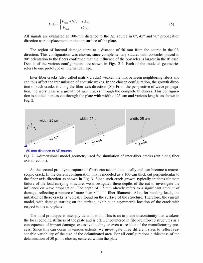
can thus affect the transmission of acoustic waves. In the chosen configuration, the growth direc-tion of such cracks is along the fiber axis direction (0°). From the perspective of wave propaga-tion, the worst case is a growth of such cracks through the complete thickness. This configura-tion is studied here as cut through the plate with width of 25 µm and various lengths as shown in Fig. 2.

Fig. 2. 3-dimensional model geometry used for simulation of inter-fiber cracks (cut along fiber axis direction).

As the second prototype, rupture of fibers can accumulate locally and can become a macro-scopic crack. In the current configuration this is modeled as a 100-µm thick cut perpendicular to the fiber axis direction as shown in Fig. 3. Since such crack growth typically initiates ultimate failure of the load carrying structure, we investigated three depths of the cut to investigate the influence on wave propagation. The depth of 0.5 mm already refers to a significant amount of damage, reflecting a rupture of more than 800,000 fiber filaments. Also, for bending loads, the initiation of these cracks is typically found on the surface of the structure. Therefore, the current model, with damage starting on the surface, exhibits an asymmetric location of the crack with respect to the mid-plane.

The third prototype is inter-ply delamination. This is an in-plane discontinuity that weakens the local bending stiffness of the plate and is often encountered in fiber-reinforced structures as a consequence of impact damage, excessive loading or even as residue of the manufacturing pro-cess. Since this can occur in various extents, we investigate three different sizes to reflect rea-sonable variability of the size of the delaminated area. For all configurations a thickness of the delamination of 50 µm is chosen, centered within the plate.

7.5 mm

20 mm

width: 25 µm

50 mm distance to AE source

z

xy

10 mm

width: 25 µm

5 mm

width: 25 µm

5

Fig. 3. 3-dimensional model geometry used for simulation of broken fibers (cut perpendicular to fiber axis direction).

Fig. 4. 3-dimensional model geometry used for simulation of inter-ply delamination (cut parallel to fiber axis direction).

Table 1. List of elastic properties used for finite element modeling.

Density [kg/m³] Elasticity Constants [GPa] T800/913 (unidirectional) 1550 C11=154.0

C12= C13=3.7 C22= C33=9.5 C23=5.2 C44=2.5 C66= C55=4.2

For accurate resolution of calculated signals, a maximum element size of 1.0 mm edge length

was chosen for tetrahedral mesh elements with quadratic order of the geometry shape functions. To resolve geometric details in narrow regions the mesh was locally refined down to a minimum edge length of 5 µm. The temporal resolution was chosen to be 100 ns and results were calculat-ed for the first 100 µs after signal excitation. Convergence of simulation results with respect to mesh resolution and temporal resolution was previously checked by subsequent refinement. To this end mesh resolution was increased to 0.5 mm edge length and temporal resolution was in-creased to 5 ns. Results of these calculations were found to have a coherence level ≥ 0.998 to the current settings within the frequency range between 1 kHz and 2 MHz. 4. Results

In the following, the influence of the modeled damage on the signal propagation is investi-gated. Figure 5 shows the Choi-Williams distribution (CWD) of the calculation result for signal

z

xy

0.500 mm

20 mm

0.250 mm

20 mm

0.125 mm

20 mm


z

xy

height:50 µm

20 mm

5 mm


height:50 µm

20 mm

10 mmheight:50 µm

20 mm

20 mm

6

propagation along the 0° axis of the unidirectional CFRP plate [Choi, 1989]. The CWD in Fig. 5-a uses a different color, frequency and time range than Fig. 5-b, which is used to emphasize the S0-mode at the initial part of the signal. To identify particular Lamb wave modes, the dispersion curves of the fundamental modes were calculated by the software package provided by [Zeyede, 2010]. As indicated by the superimposed dispersion curves for the S0-mode at 100 mm and 300 mm source distance, the S0-mode is reflected at the edge of the plate in x-direction and is detected more than once. The CWD result of the A0-mode shown in Fig. 3-b agrees well with the calculated result of the A0 dispersion curve for 100 mm distance. The small dips in the curve seen at 52 µs and 62 µs are caused by multiple reflections of the S0-mode, which has been re-flected at all edges of the plate at this time. The calculation results for the pure CFRP plate in Fig. 5 will act as a reference case to evaluate the influence of any damage modeled within the propagation path. A comparison of the calculated wave-fields will be made in section 5.

Fig. 5. Simulation results of signal propagation at 100 mm distance along 0° direction in unidi-rectional CFRP. Truncated time scale shows S0-mode (a) and full time scale shows A0-mode (b).

0200400600800

100012001400160018002000

(a)

Fre

quen

cy [k

Hz]

0.000

0.004000

0.008000

0.01200

0.01600

0.02000

CFRP Reference

edge reflection

0.00 0.01 0.02 0.03 0.04 0.05

-10-505

10

Dis

plac

emen

t [fm

]

Time [ms]

S0-mode (100mm) S0-mode (300mm)

0

200

400

600

800

1000

(b)

Fre

quen

cy [k

Hz]

0.000

4.000

8.000

12.00

16.00

20.00

CFRP Reference

0.000 0.025 0.050 0.075 0.100-0.10

-0.05

0.00

0.05

0.10

Dis

plac

emen

t [nm

]

Time [ms]

A0-mode (100mm) S0-mode (100mm)

7

4a. Inter-fiber cracks Inter-fiber cracks are one of the basic damage types found in fiber-reinforced composites.

These are cracks with propagation direction parallel to the fiber axis direction. Since the strength of the direction perpendicular to the fiber axis is the weak link between the fibers, this type of damage is observed frequently in composite structures. In the current configuration, the inter-fiber crack is modeled as crack-through process, i.e. the crack reaches from the top to the bottom of the plate. The length of the inter-fiber crack is varied between 5 mm and 20 mm to cover a broad range of macroscopic crack sizes.

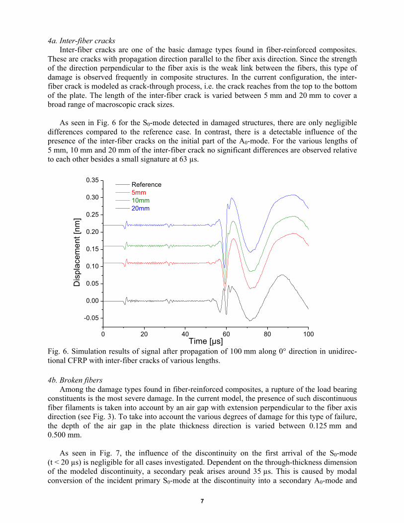
As seen in Fig. 6 for the S0-mode detected in damaged structures, there are only negligible

differences compared to the reference case. In contrast, there is a detectable influence of the presence of the inter-fiber cracks on the initial part of the A0-mode. For the various lengths of 5 mm, 10 mm and 20 mm of the inter-fiber crack no significant differences are observed relative to each other besides a small signature at 63 µs.

Fig. 6. Simulation results of signal after propagation of 100 mm along 0° direction in unidirec-tional CFRP with inter-fiber cracks of various lengths. 4b. Broken fibers

Among the damage types found in fiber-reinforced composites, a rupture of the load bearing constituents is the most severe damage. In the current model, the presence of such discontinuous fiber filaments is taken into account by an air gap with extension perpendicular to the fiber axis direction (see Fig. 3). To take into account the various degrees of damage for this type of failure, the depth of the air gap in the plate thickness direction is varied between 0.125 mm and 0.500 mm.

As seen in Fig. 7, the influence of the discontinuity on the first arrival of the S0-mode

(t < 20 µs) is negligible for all cases investigated. Dependent on the through-thickness dimension of the modeled discontinuity, a secondary peak arises around 35 µs. This is caused by modal conversion of the incident primary S0-mode at the discontinuity into a secondary A0-mode and

0 20 40 60 80 100

-0.05

0.00

0.05

0.10

0.15

0.20

0.25

0.30

0.35 Reference 5mm 10mm 20mm

Dis

plac

emen

t [nm

]

Time [µs]

8

into a secondary S0-mode (see Fig. 9 and Fig. 10, also [Sause, 2012d]). The later parts of the signal (t > 40 µs) are also affected by this interaction, which causes a superposition of the inci-dent A0-mode with the multiple reflections of the secondary modes. It is worth noting that the model is energy conservative. Still, the calculated amplitude of the signals is distinctly different. This is solely caused by the presence of the broken fibers, which cause a preferential scattering of the displacement field, which transfers energy from the in-plane displacement to the out-of-plane displacement.

Fig. 7. Simulation results of signal after propagation of 100 mm along 0° direction in unidirec-tional CFRP with broken fibers modeled with various dimensions. 4c Inter-ply delamination

Inter-ply delamination is one of the most common types of damage found in fiber-reinforced composites, since it is often caused by local impact or as residue of a manufacturing error. Dur-ing mechanical testing of fiber-reinforced structures, delamination can evolve step by step and can affect the elastic properties along the signal propagation path. Thus, the influence of delami-nation on the detected AE signals is of considerable interest. To resemble the variety of dimen-sions of inter-ply delamination, the size of the delaminated area in the in-plane direction was varied between 5 mm and 20 mm (see Fig. 4).

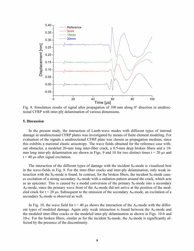
Figure 8 shows the calculated signals for all three inter-ply delamination sizes investigated

and the reference signal for comparison. For the S0-mode there are only negligible differences observed to the reference case. Since propagation of the S0-mode is dominated by the in-plane stiffness, this is explained by considering a multi-layer specimen composed of 950 µm CFRP and 50 µm air. The in-plane stiffness of such a plate is as close as 95 % of the stiffness of a pure 1000-µm CFRP plate. A larger influence is observed for the propagation behavior of the A0-mode. The shape and intensity of the A0-modes differ from the reference signal due to the change of local bending stiffness as introduced by the inter-ply delamination. With increasing size of the inter-ply delamination, the deviation compared to the reference case increases as well.

0 20 40 60 80 100

-0.05

0.00

0.05

0.10

0.15

0.20

0.25

0.30

0.35

0.40

0.45

0.50 Reference 0.125mm 0.250mm 0.500mm

Dis

plac

emen

t [nm

]

Time [µs]

9

Fig. 8. Simulation results of signal after propagation of 100 mm along 0° direction in unidirec-tional CFRP with inter-ply delamination of various dimensions. 5. Discussion

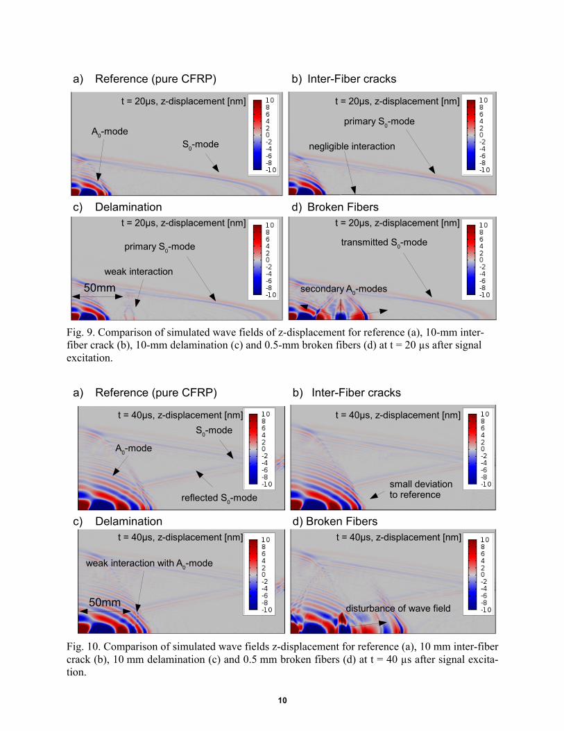
In the present study, the interaction of Lamb-wave modes with different types of internal damage in unidirectional CFRP plates was investigated by means of finite element modeling. For evaluation of the signals a unidirectional CFRP plate was chosen as propagation medium, since this exhibits a maximal elastic anisotropy. The wave fields obtained for the reference case with-out obstacles, a modeled 20-mm long inter-fiber crack, a 0.5-mm deep broken fibers and a 10-mm long inter-ply delamination are shown in Figs. 9 and 10 for two distinct times t = 20 µs and t = 40 µs after signal excitation.

The interaction of the different types of damage with the incident S0-mode is visualized best in the wave-fields in Fig. 9. For the inter-fiber cracks and inter-ply delamination, only weak in-teraction with the S0-mode is found. In contrast, for the broken fibers, the incident S0-mode caus-es excitation of a strong secondary A0-mode with a radiation pattern around the crack, which acts as an epicenter. This is caused by a modal conversion of the primary S0-mode into a secondary A0-mode, since the primary wave front of the A0-mode did not arrive at the position of the mod-eled crack for t < 20 µs. Subsequent to the emission of the secondary A0-mode, an excitation of a secondary S0-mode is observed as well.

In Fig. 10, the wave field for t = 40 µs shows the interaction of the A0-mode with the differ-

ent types of modeled damage. Again only weak interaction is found between the A0-mode and the modeled inter-fiber cracks or the modeled inter-ply delamination as shown in Figs. 10-b and 10-c. For the broken fibers, similar as for the incident S0-mode, the A0-mode is significantly af-fected by the presence of the discontinuity.

0 20 40 60 80 100

-0.05

0.00

0.05

0.10

0.15

0.20

0.25

0.30

0.35

0.40 Reference 5mm 10mm 20mm

Dis

plac

emen

t [nm

]

Time [µs]

10

Fig. 9. Comparison of simulated wave fields of z-displacement for reference (a), 10-mm inter-fiber crack (b), 10-mm delamination (c) and 0.5-mm broken fibers (d) at t = 20 µs after signal excitation.

Fig. 10. Comparison of simulated wave fields z-displacement for reference (a), 10 mm inter-fiber crack (b), 10 mm delamination (c) and 0.5 mm broken fibers (d) at t = 40 µs after signal excita-tion.

S0-modeA0-mode

primary S0-mode

negligible interaction

primary S0-mode transmitted S0-mode

secondary A0-modes

weak interaction

a) b)

c) d)

Reference (pure CFRP) Inter-Fiber cracks

Delamination Broken Fibers

t = 20µs, z-displacement [nm] t = 20µs, z-displacement [nm]


50mm

S0-mode

A0-mode

small deviation to reference

disturbance of wave field

weak interaction with A0-mode



reflected S0-mode

Reference (pure CFRP) Inter-Fiber cracks

Delamination

a) b)

c) d) Broken Fibers

50mm

11

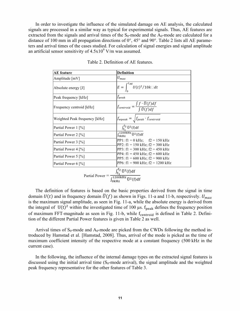
In order to investigate the influence of the simulated damage on AE analysis, the calculated signals are processed in a similar way as typical for experimental signals. Thus, AE features are extracted from the signals and arrival times of the S0-mode and the A0-mode are calculated for a distance of 100 mm in all propagation directions of 0°, 45° and 90°. Table 2 lists all AE parame-ters and arrival times of the cases studied. For calculation of signal energies and signal amplitude an artificial sensor sensitivity of 4.5x109 V/m was assumed.

Table 2. Definition of AE features.

AE feature Definition Amplitude [mV] 𝑈!"#

Absolute energy [J] 𝐸 = 𝑈 𝑡 ! 10𝑘�𝑑𝑡!!"

!

Peak frequency [kHz] 𝑓!"#$

Frequency centroid [kHz] 𝑓!"#$%&'( =𝑓 ∙ 𝑈(𝑓)𝑑𝑓𝑈 𝑓 𝑑𝑓

Weighted Peak frequency [kHz] 𝑓!"#$% = 𝑓!"#$ ∙ 𝑓!"#$%&'(

Partial Power 1 [%] !! ! !"!!!!

!! ! !"!"##$%&!"#$

PP1: f1 = 0 kHz; f2 = 150 kHz PP2: f1 = 150 kHz; f2 = 300 kHz PP3: f1 = 300 kHz; f2 = 450 kHz PP4: f1 = 450 kHz; f2 = 600 kHz PP5: f1 = 600 kHz; f2 = 900 kHz PP6: f1 = 900 kHz; f2 = 1200 kHz

Partial Power 2 [%]

Partial Power 3 [%]

Partial Power 4 [%]

Partial Power 5 [%]

Partial Power 6 [%]

Partial Power = !! ! !"!!

!!

!! ! !"!"##$%&!"#$

The definition of features is based on the basic properties derived from the signal in time

domain 𝑈 𝑡 and in frequency domain 𝑈 𝑓 as shown in Figs. 11-a and 11-b, respectively. 𝑈!"# is the maximum signal amplitude, as seen in Fig. 11-a, while the absolute energy is derived from the integral of U t ! within the investigated time of 100 µs. f!"#$ defines the frequency position of maximum FFT-magnitude as seen in Fig. 11-b, while f!"#$%&'( is defined in Table 2. Defini-tion of the different Partial Power features is given in Table 2 as well.

Arrival times of S0-mode and A0-mode are picked from the CWDs following the method in-

troduced by Hamstad et al. [Hamstad, 2008]. Thus, arrival of the mode is picked as the time of maximum coefficient intensity of the respective mode at a constant frequency (500 kHz in the current case).

In the following, the influence of the internal damage types on the extracted signal features is discussed using the initial arrival time (S0-mode arrival), the signal amplitude and the weighted peak frequency representative for the other features of Table 3.

12

Fig. 11. Extraction of features from acoustic emission signals in time (a) and frequency domain (b).

t0

tAE

threshold level

Umax

0.00 0.02 0.04 0.06 0.08 0.10

-0.010

-0.005

0.000

0.005

0.010

(a)

Am

plitu

de [m

V]

Time [ms]

13

Table 3. Values of AE features extracted from the calculated signals in various propagation di-rections. C

onfiguration

Arrival tim

e S0 [ µs]

Arrival tim

e A0 [µs]

Am

plitude [mV

]

Absolute energy [nJ]

Peak frequency [kH

z]

Weighted Peak fre-

quency [kHz]

Frequency centroid [kH

z]

Partial Power 1[%

]

Partial Power 2 [%

]

Partial Power 3 [%

]

Partial Power 4 [%

]

Partial Power 5 [%

]

Partial Power 6 [%

]

Reference 0° 1 9.2 81.6 342.5 23.4 39.1 124.5 396.5 59.5 13.3 13.7 7.0 10.9 1.6 45° 11 23.8 90.2 30.5 23.6 127.0 232.4 425.3 38.6 21.2 17.8 9.2 23.4 2.3 90° 21 33.5 44.6 24.9 23.6 293.0 504.9 870.0 16.0 18.4 17.9 8.9 2.2 15.5 Inter-fiber cracks 5mm-0° 2 9.3 91.7 388.2 55.6 29.3 72.3 178.4 77.6 12.8 4.3 1.7 11.8 1.5 5mm-45° 12 24.8 90.2 32.3 55.8 87.9 229.9 601.4 30.6 15.3 23.1 17.0 15.6 2.2 5mm-90° 22 35.6 37.0 26.5 55.8 117.2 234.2 468.2 20.9 23.6 24.1 14.3 2.3 1.5 10mm-0° 3 9.2 91.8 498.3 58.0 29.3 73.7 185.5 68.7 15.4 8.7 3.8 8.0 1.1 10mm-45° 13 24.7 90.2 31.4 58.2 87.9 223.7 569.3 40.6 21.6 18.0 9.4 13.6 2.4 10mm-90° 23 31.9 40.8 24.2 58.3 263.7 353.6 474.2 22.0 24.4 25.1 13.7 2.1 1.2 20mm-0° 4 8.9 91.5 556.4 64.1 29.3 71.7 175.7 66.3 17.0 9.6 4.2 8.5 0.9 20mm-45° 14 23.1 90.2 32.0 64.4 87.9 225.6 579.2 41.5 20.8 17.6 9.2 18.5 2.5 20mm-90° 24 29.3 40.6 30.4 64.4 263.7 338.7 435.0 19.9 23.0 24.4 13.3 3.6 0.9 Fiber breaks 0.125mm-0° 5 9.4 90.0 369.7 44.1 29.3 70.2 168.1 77.9 7.7 5.9 3.6 11.9 1.3 0.125mm-45° 15 25.6 90.2 29.8 44.3 87.9 229.1 597.3 42.2 16.9 18.1 8.4 19.0 2.5 0.125mm-90° 25 31.8 37.0 30.0 44.3 439.5 438.8 438.2 16.7 20.6 27.5 15.4 4.9 0.8 0.25mm-0° 6 9.4 90.0 533.7 54.0 19.5 64.8 214.9 63.0 13.3 11.1 6.8 16.5 0.9 0.25mm-45° 16 25.3 92.5 37.5 54.2 87.9 227.2 587.6 36.6 15.0 18.1 11.7 19.0 2.2 0.25mm-90° 26 31.7 36.9 29.7 54.3 439.5 423.6 408.3 17.0 20.0 25.0 17.0 6.0 1.0 0.5mm-0° 7 9.4 90.8 993.1 122.0 9.8 60.3 372.9 50.0 19.0 15.0 9.0 10.6 1.0 0.5mm-45° 17 23.7 92.5 45.3 122.0 87.9 220.5 553.1 37.3 15.1 22.9 12.3 21.0 1.9 0.5mm-90° 27 30.9 41.0 32.8 122.0 439.5 451.6 464.0 15.0 18.0 24.0 21.0 3.0 1.0 Delamination 5mm-0° 8 9.4 92.3 358.0 39.5 29.3 85.7 250.8 81.0 9.0 3.0 2.0 10.0 2.0 5mm-45° 18 24.6 92.5 34.1 39.7 97.7 249.3 636.7 40.9 19.0 17.1 10.2 27.0 2.9 5mm-90° 28 29.7 36.8 31.4 39.8 293.0 368.1 462.6 14.0 18.0 22.0 17.0 4.0 1.0 10mm-0° 9 9.4 102.0 322.1 35.4 39.1 128.3 421.6 76.0 11.0 4.0 3.0 19.9 3.0 10mm-45° 19 24.8 39.2 35.1 35.7 97.7 247.3 626.4 36.0 20.0 12.7 9.0 29.0 2.3 10mm-90° 29 32.0 68.6 24.6 35.8 293.0 384.0 503.3 16.0 19.0 20.0 15.0 4.0 1.4 20mm-0° 10 9.4 42.0 523.6 59.0 39.1 146.8 552.0 62.0 18.0 9.0 4.0 7.5 3.0 20mm-45° 20 24.2 90.2 40.7 59.4 87.9 226.2 582.2 42.6 22.5 18.0 6.8 19.0 2.6 20mm-90° 30 29.3 71.0 31.1 59.5 175.8 281.1 449.5 21.0 23.0 21.0 14.0 10.9 2.0

14

5a. Influence on arrival time In order to obtain valid source locations, a proper determination of the initial arrival time is a

key requirement for most of the currently used localization algorithms. The significant influence of the various internal damage types on the propagation behavior of the signals was already demonstrated in section 4. In Fig. 12, the extracted initial arrival times are shown for all damage configurations and the reference case in 0°, 45° and 90° propagation direction. The largest influ-ence of the internal damage types is found for the 90° propagation direction, which demon-strates, that the complete wave-field is affected by the presence of the damage and not solely the part of the wave propagating through the obstacle (0° direction).

Based on the maximum deviation of 4.2 µs to the reference case of the calculated arrival time

of the S0-mode in 90° propagation direction, a corresponding error of localization in the range of several centimeters can be expected. The estimation is based on the calculated group velocity of the S0-mode in 90° propagation direction.

A significantly larger influence was found for the arrival time of the A0 mode. Due to modal

conversion occurring at the internal damage, the arrival of the first detectable A0-mode is 48.6 µs ahead compared to the reference case in one configuration. However, this is not the arrival of the primary A0 mode as discussed before. For the majority of the cases studied, the arrival times of the A0 mode are within 10 µs difference to the reference case. Consequently, for localization methods using arrival times of both fundamental Lamb wave modes, the observed difference in arrival time of the A0 mode might have a large impact as well.

Fig. 12. Calculated arrival time of S0-mode for the various configurations of internal damage in comparison to the reference case for 0°, 45° and 90° propagation direction.

0 5 10 15 20 25 305

10

15

20

25

30

35

40

Reference case Inter-Fiber cracks Broken Fibers Inter-ply Delamination

90°

45°

S0 a

rriv

al ti

me

[µs]

configuration

0°

15

5b. Influence on signal features For source identification procedures one approach is the use of parameter-based pattern

recognition [Sause, 2010c, Sause, 2010a, Sause, 2012a]. Since cracks and delamination are likely to evolve between AE source positions and the position of detection during specimen loading, their influence on the transmitted Lamb waves has to be understood thoroughly.

From the list of calculated features given in Table 2, some were found to deviate more than

100 % from the reference case. One example is the signal amplitude values shown in Fig. 13 for each configuration, evaluated in 0°, 45° and 90° propagation directions. Compared to the refer-ence case (red), the signals passing through the damaged region experience large changes of their signal amplitude. This is due to the modal conversion at the damage position, and the scattering introduced by some of the damage types. These effects are not taken into account by the conven-tional definitions for calculation of signal amplitude or AE signal energies as given in Table 2. Except for configuration 7, the overall deviation of amplitude values was found to be within ± 0.25 V (i.e. ± 5 dBAE) to the reference case. Compared to the ± 3 dBAE recommendation of ASTM E 2191 for sensor replacement this amplitude range is well within typically encountered uncertainties of measurement setups used.

Fig. 13. Calculated signal amplitude of signals for the various configurations of internal damage in comparison to the reference case for 0°, 45° and 90° propagation direction.

The calculated weighted Peak-Frequency for the signals of different damage configurations and the reference case are shown in Fig. 14 for 0°, 45° and 90° propagation directions. Depend-ent on the propagation angle, different values for the weighted peak frequency are observed. This is caused by the asymmetric propagation of Lamb-wave modes in the unidirectional plate mod-eled herein. Similar to the signal amplitude, deviations compared to the reference case are up to 100 %. Again, features evaluated in all propagation directions are affected by the presence of the modeled damage types. The range of feature values seems unacceptably high in order to perform

0 5 10 15 20 25 300.000.010.020.030.040.050.060.07

0.30.40.50.60.70.80.91.0

Reference case Inter-Fiber cracks Broken Fibers Inter-ply Delamination

ampl

itude

[V]

configuration

16

valid source identification based on frequency features, since the modeled source type is identi-cal for all cases studied.

Fig. 14. Calculated weighted peak frequency of signals for the various configurations of internal damage in comparison to the reference case for 0°, 45° and 90° propagation direction.

However, for pattern recognition methods, there is a typical experimentally encountered dis-tribution range for an individual feature. This is demonstrated in Fig. 15. Here, the experimental-ly detected signal features of a double cantilever beam experiment including their classification into matrix cracking, interfacial failure and fiber breakage are shown. Details of the experimental setup are found in [Sause, 2010d, Sause, 2012b], while references [Sause, 2010c, Sause, 2012a] focus on the underlying methodology. The black data points are the resulting feature values of the current simulation work with black circles marking the signals propagation direction. For the current evaluation along one propagation direction, the feature range observed is quite compara-ble to the typical extent of one cluster observed for a particular failure mechanism (i.e. matrix cracking, interfacial failure or fiber breakage). Thus, the presence of a failure type, as modeled herein, is expected to increase the dimensions of the cluster belonging to a particular failure type.

6. Conclusions

Within this study the influence of internal damage in fiber-reinforced composites on signal propagation of Lamb waves was investigated. For the present study a unidirectional fiber-reinforced plate was studied, including embedded models for inter-fiber cracks, broken fibers and inter-ply delamination located in the 0° direction of the plate.

Overall, a significant influence on the signals from all damage types was observed that is well detectable with piezoelectric sensors, and thus a feasible approach for SHM utilizing guided wave monitoring.

0 5 10 15 20 25 300

100

200

300

400

500 Reference case Inter-Fiber cracks Broken Fibers Inter-ply Delamination

Wei

gted

Pea

k Fr

eque

ncy

[kH

z]

configuration

0°

45°

90°

17

Fig. 15. Diagram of weighted peak frequency vs. partial power 3 of experimental measurement of double cantilever beam specimen [Sause, 2010d] compared to positions of features extracted from simulated signals for 0°, 45° and 90° propagation direction (all configurations).

For AE analysis, the largest impact is expected for source localization routines, since the in-ternal damage types can act as virtual AE source caused by modal conversion effects. This sig-nificantly alters the emitted wave field of the original source and may even affect the initial arri-val time of the different wave modes, causing substantial errors during source localization.

Also, energetic features and frequency features extracted from the Lamb-wave signals are in-

fluenced by the presence of internal damage. In some configurations, the influence on a particu-lar feature value was found to be very significant. However, the overall range of values of the extracted features is comparable to ranges where pattern recognition approaches still can lead to valid classifications of source mechanisms. In contrast, the evaluation of signals with different observation angles relative to the source positions might cause a larger impact with respect to the accuracy of pattern recognition methods. Acknowledgment

I would like to thank Marvin A. Hamstad for the possibility to discuss AE sensing technolo-gies and signal propagation in fiber-reinforced polymers. Literature [Castaings, 2004] M. Castaings, C. Bacon, B. Hosten and M. V. Predoi (2004), J.

Acoust. Soc. Am., 115:3, 1125-1133. [Choi, 1989] H. Choi, W. Williams, IEEE Transactions on Acoustics, Speech and

Signal Processing, 37:6, 862-872.

0 100 200 300 400 500 600 700 800 900 10000

20

40

60

80

100

45°90°

Cluster 0 (Matrix cracking) Cluster 1 (Interface failure) Cluster 2 (Fiber breakage)

Par

tial P

ower

3 [%

]

Weighted Peak-Frequency [kHz]

0°

18

[Gary, 1994] J. Gary and M. A. Hamstad (1994), J. Acoustic Emission, 12:3-4, 157-170.

[Hamstad, 2002] M.A. Hamstad, A. O’Gallagher, J. Gary, J. Acoustic Emission, 12:3-4, 157-170.

[Hamstad, 2008] M.A. Hamstad, J. Acoustic Emission, 26, 40-59. [Lamb, 1917] H Lamb, ‘On Waves in an Elastic Plate’, Proceedings of the Royal

Society of London Series A Containing Papers of a Mathematical and Physical Character, Vol 93, pp 114-128, 1917.

[Lowe, 1995] M. Lowe, IEEE Transactions on Ultrasonics Ferroelectrics and Fre-quency Control, 42:4, 525-542.

[Raghavan, 2007] A. Raghavan, C. Cesnik,The Shock and Vibration Digest, 39, 91-114.

[Sause, 2010a] M. G. R. Sause and S. Horn (2010), J. Nondest. Eval., 29:2, 123-142. [Sause, 2010b] M. G. R. Sause and S. Horn (2010), J. Acoustic Emission, 28, 142-

154. [Sause, 2010c] M. G. R. Sause (2010), Identification of failure mechanisms in hy-

brid materials utilizing pattern recognition techniques applied to acoustic emission analysis, PhD-thesis, mbv-Verlag, Berlin.

[Sause, 2010d] M. G. R. Sause and S. Horn, Influence of Specimen Geometry on Acoustic Emission Signals in Fiber Reinforced Composites: FEM-Simulations and Experiments, 29th European Conference on Acoustic Emission Testing, Vienna 09/2010

[Sause, 2012a] M.G.R. Sause, A. Gribov, A.R. Unwin, S. Horn, Pat. Rec. Letters, 33:1, 17-23.

[Sause, 2012b] M.G.R. Sause, T. Müller, A. Horoschenkoff, S. Horn, Comp. Sci. Technol., 72, 167-174.

[Sause, 2012c] M.G.R. Sause, M.A. Hamstad, S. Horn, Sens. Act. A., 184, 64-71. [Sause, 2012d] M. G. R. Sause, S. Horn, Influence of Internal Discontinuities on

Ultrasonic Signal Propagation in Carbon Fiber Reinforced Plastics, 30thEuropean Conference on Acoustic emission Testing, Granada 09/2012

[Wang, 2007] L. Wang, F. Yuan, Comp. Sci. Technol., 67, 1370-1384. [Zeyede, 2010] R. Zeyede,Notes on orthotropic Lamb waves, Technion - Israel Insti-

tute of Technology, http://mercurial.intuxication.org/hg/elasticsim/


In-Flight Fatigue Crack Growth Monitoring in a Cessna T-303 Crusader Vertical Tail

Eric v. K. Hill1 and Christopher L. Rovik2

1 Aura Vector Consulting, 3041 Turnbull Bay Road, New Smyrna Beach, FL 32168 2 Toyota Technical Center, 8777 Platt Road, Saline, MI 48176

Abstract This research involved the in-flight monitoring of fatigue crack growth in the vertical tail of a Cessna T-303 Crusader twin-engine aircraft. A notched 7075-T6 aluminum aircraft channel beam support structure was cyclically tested in the laboratory. Acoustic emission (AE) data were taken during these fatigue tests, which were subsequently sorted into three failure mecha-nisms: fatigue cracking, plastic deformation, and rubbing noise. These data were then used to train a Kohonen self-organizing map (SOM) neural network. At this point, a similar channel beam support structure was installed as a redundant structural member between the ribs in the vertical tail of the T-303 aircraft. AE data were subsequently gathered from initial taxiing and takeoff to the final approach and landing. The AE data recorded during the in-flight tests were then classified using the laboratory trained SOM neural network into the three above mentioned mechanisms. From this it was determined that plastic deformation occurred throughout all re-gions of flight but was most prevalent during taxi operations, fatigue crack growth activity oc-curred mostly during flight operations -- particularly during roll and Dutch roll maneuvers -- while the mechanical rubbing noise occurred mainly during flight with very little occurring dur-ing taxi. The success of the SOM classification of failure mechanisms indicated that the proto-type in-flight structural health monitoring system for aging aircraft was highly successful at cap-turing fatigue crack growth data. It is envisioned that the application of such structural health monitoring systems in aging aircraft could warn of impending failure and allow for replacement of parts when needed rather than at conservatively calculated intervals. As such, continuation of this research should eventually help to minimize maintenance costs and extend the service lives of aging aircraft. Keywords: Aging aircraft, in-flight fatigue crack monitoring, Kohonen self-organizing map, neural network, structural health monitoring Introduction Fatigue Cracking in Aircraft Aircraft today typically are expected to last longer than automobiles. This is due to many factors, including the cost of the aircraft, government regulations, and the dramatic consequences of failure. There are many problems that arise from the fact that aircraft are expected to last so long. Perhaps the major source of problems, which is the subject of this research, is the presence and growth of fatigue cracks. The ability to repair damage from fatigue cracks has not been a problem, but the detection and monitoring of fatigue crack growth has proven to be a real chal-lenge. Fatigue cracking is the brittle fracture that results from cyclic loading below the yield strength of a normally ductile metal. The highly concentrated stresses at the crack tip result in the formation of a heart-shaped plastically deformed zone ahead of the crack. This plastic zone strain hardens with cyclic loading and fractures when the ductility of the metal has been exhaust-

20

ed, thereby extending the crack. This fatigue crack growth process repeats itself over and over again until final failure of the part. Aircraft experience different types of fatigue loadings. Takeoffs and landings are very fun-damental types of cyclic loadings on aircraft. Cabin pressurization is also a type of cyclic load-ing, since the fuselage of an aircraft is a large pressure vessel that undergoes a breathing process as the plane pressurizes and depressurizes to accommodate passengers at varying altitudes. Vi-bration due to atmospheric turbulence and engines is also a major cause of fatigue cracking in aircraft. Thus, all aircraft develop fatigue cracks over time. Detecting fatigue cracks in aircraft structures is important because, if left unchecked, the cracks will eventually reach critical length, at which point they progress to catastrophic failure within a relatively short period of time. As a structure with a crack is cycled, the crack will grow until it is stopped -- for instance by grain boundaries -- but it will then typically change direc-tions within a few cycles and continue to progress to failure. The affected parts must be replaced before this happens. Currently this is accomplished at conservatively calculated intervals based on linear elastic fracture mechanics. However, it would be beneficial to develop a system to monitor the growth of fatigue cracks so that replacements are installed only when needed, rather than at calculated intervals that are of necessity, highly conservative. Detecting Fatigue Cracks There are several nondestructive testing methods commonly used to detect fatigue cracks in aircraft. Two of the most common are eddy current testing and radiographic testing. The main disadvantages to eddy current and radiographic testing are that they are both time consuming and therefore very expensive. But more than that, these two techniques oftentimes require disassem-bly of the structure in question to obtain access for the inspection, and as such, crack growth monitoring is at best intermittent rather than continuous. The ability to detect a growing fatigue crack and identify its location is fundamental to reducing the maintenance costs associated with aircraft ownership and at the same time improving aircraft safety. Acoustic emission (AE) nondestructive testing has been employed previously for continuous in-flight monitoring of aircraft fatigue crack signals [1-5]. In order to detect fatigue crack growth in an in-flight environment, it is necessary to determine the characteristics of the cracking signal. The problem arises from the fact that amongst the crack signals, there also exist signals due to plastic deformation and mechanical noise. Neural networks have been employed herein to separate these signals and classify them as to the appropriate mechanism. The test bed used for the in-flight fatigue crack growth monitoring was the vertical tail of a Cessna T-303 Crusader aircraft shown in Fig. 1. It is interesting to note here that the crack growth data acquisition for this aircraft was prematurely terminated because of the unexpected discovery of fatigue cracks in its wing ribs. This resulted in the decision to sell the aircraft rather than repair it; consequently, the planned data acquisition from the controlled fatigue cracking in the vertical tail was cut short. Ironically, such an acoustic crack detection system as utilized in this research, when fully developed, could have monitored those wing rib fatigue cracks in flight to ensure safety while the airplane was being returned for repairs.

21

Fig. 1. Cessna T-303 Crusader test bed aircraft. The experimental research associated with this study consisted of two segments. The first segment dealt with the testing of a fatigue crack growth specimen in a controlled laboratory envi-ronment. The second segment of the research involved the testing of a similar specimen installed in the vertical tail of the Cessna T-303 Crusader test bed aircraft. The in-flight specimen was a redundant structure, as it was not installed to replace any structure of the aircraft but simply to provide a structure that could undergo fatigue cracking without compromising the structural in-tegrity of the aircraft. Data were taken during various flight regimes, including taxi, takeoff, steady level flight, rolls, and Dutch rolls. The purpose of the two roll maneuvers was to impose significant bending loads on the vertical tail which would hopefully induce fatigue crack growth in the notched portion of the redundant specimen. Acoustic Emission Acoustic emission nondestructive testing was the tool used in this research to monitor fatigue cracking. Acoustic emissions are typically referred to as sound waves, but more appropriately, they are the stress waves that propagate throughout a medium as a result of a sudden release of energy [6]. The purpose of this study was to identify and monitor the growth of fatigue cracks; therefore, the waveforms associated with a fatigue cracking were of particular interest here. The research presented herein was based on identifying and monitoring fatigue crack growth in the redundant internal structure mounted between the ribs in the vertical tail. A concurrent research project involved AE monitoring of fatigue cracking in the engine cowling of a Piper PA-28 Cadet general aviation aircraft [7]. The results of these two research projects will provide the basis for the development of an operational, in-flight acoustic emission fatigue crack growth monitoring system for aging aircraft. Experimental Procedure Data Acquisition and Digital Signal Processing Digital signal processing is the process by which an analog waveform is converted into a dis-crete approximation of the analog signal. An understanding of the data acquisition system is necessary in order to understand the process of converting an analog signal into a digital repre-sentation.

22

Fig. 2. AE data acquisition system. As shown in the block diagram of Fig. 2, included in the AE data acquisition system is a fil-ter for each transducer used. It is a critical first step to determine all possible sources of back-ground noise so that these sources, where possible, can be filtered out a priori from the rest of the signals. Many sources of background noise were identified for both the laboratory and the in-flight environment and are summarized in Table 1. The laboratory test involved testing a fatigue specimen attached to a cyclic MTS tensile test machine as well as a VTS shaker table. The many possible sources of background noise in the lab were identified and filtered out. For example, high frequency electromagnetic interference (EMI) signals can be filtered out using a low pass filter. The presence of mechanical noise was very obvious in the laboratory during the tests associ-ated with the MTS machine. The MTS machine operates using a hydraulic system to deliver a force to the collar to which the specimen was attached. Some of these concerns were alleviated by the fact that the hydraulic servo was mechanically isolated from the actual test platform by the use of hoses rather than mechanical connections. Nevertheless, there was still a significant amount of hydraulic noise that had to be filtered out. Also the fluorescent lighting in the lab emitted a 60 Hz wave, which can impact the data acquisition system through radiation and sim-ple electrical induction. Both of these noise sources were eliminated through the use of high-pass filters. There was also a significant amount of mechanical noise emanating from the structure itself. These sources of noise were mechanisms such as rivet fretting and bearing failure in the bolt holes. The goal of our test was not to eliminate these signals, as their presence in the airplane is unavoidable; hence, they were not filtered out. However, there were other sources of mechanical noise present, which were not necessarily directly associated with the test structure. Due to the fact that the MTS tensile test machine secures a specimen by using a hydraulically operated grip, there was noise associated with the plastic deformation between the specimen and the grip. A high-pass filter was used to eliminate as much of this mechanical noise as possible, while not removing noise associated with rivet fretting and bearing failure [8]. Similar mechanical noises were present in the VTS shaker table tests. Moreover, there was also a substantial amount of noise present during the in-flight test. There was EMI noise from the strobe light tail beacon. There was also mechanical noise from the control cables that run through the empennage to operate the control surfaces. In addition, the noise associated with turbulent airflow over the empennage was a source of continuous noise that was very difficult to eliminate.

23

Table 1. Sources of background noise.

Noise Source Noise Type Noise Source Noise TypeFluorescent Lights EMI Tail Beacon EMIMTS Hydraulics Hydraulic Noise Control Surfaces Mechanical Noise

Grip Rubbing Mechanical Noise Interface Rubbing Mechanical NoiseRivet Fretting Mechanical Noise Rivet Fretting Mechanical Noise

Bearing Failure Mechanical Noise Bearing Failure Mechanical Noise

Laboratory Test In-Flight Test

A graphical representation of AE activity is quite useful in qualitatively examining the data gathered during the tests. There are several combinations of the six parameters recorded, in ad-dition to the variants derived from these parameters, which are commonly used to determine the presence of various mechanisms in a data set (Fig. 3). Analysis of these plots provided evidence that there were at least three distinctly discernable mechanisms. The data acquisition software provided real-time analysis of the AE data. Thus, it was possi-ble to study the incoming signals as they occurred. This is quite beneficial for monitoring struc-tures. For example, in the AE analysis of the structural integrity of pressure vessels it is possible to determine from the real-time analysis of data that a leak is occurring and that failure is immi-nent [6]. Such information is invaluable because it allows the operator to relieve pressure before irreparable damage occurs. The same technology was beneficial for this research, as the goal was to identify and monitor in-flight fatigue crack growth in real time. The detection of a critical defect at the earliest possible time is the key to saving lives and property and minimizing maintenance costs.

Fig. 3. Graphical representation of AE data.

24

The four scatter plots that were used here to qualitatively discern the presence of different AE mechanisms are shown in Fig. 3. These include duration vs. amplitude (Fig. 3a), counts vs. energy (Fig. 3b), duration vs. counts (Fig. 3c), and hits vs. amplitude (Fig. 3d). The first three plots show what appear to be three clearly discernable mechanisms. Analysis of the fourth graph, hits vs. amplitude, would require classification and separation of the various source mech-anism groupings, which typically overlap in the amplitude domain. Neural Networks Neural networks get their name from the fact that they closely mimic the operation of the human brain, the most powerful computing device known to man. The key component of the human brain that facilitates the processing of data is the neuron. This biological neuron is a for-midable processor, composed of dendrites, soma, and axon [9]. Dendrites are the data collection components of the neuron, as they gather data from other neurons. The main purpose of the so-ma is to sum the incoming data; hence, the name soma, for sum. The axon is the transmitter of the neuron. Its purpose is to send a signal to other neurons. There are quite a few similarities between biological neurons and artificial neurons, which are at the heart of neural networks. Be-cause of the fact that a method for classification of signals was required, it was necessary to choose an artificial neural network that was well suited to the task. The Kohonen self-organizing map (SOM) was chosen because of its excellent classification ability even when several varia-bles (n-dimensional data) are involved. The Kohonen Self-Organizing Map (SOM) In order to understand how classification is accomplished, it is necessary to understand how a neural network operates. The most basic aspect of a neural network is that it accepts input data through input neurons. In the case of the Kohonen self-organizing map used for the fatigue crack analysis, the AE parameters recorded through digital signal processing were applied to the input neurons. The six input neurons are the AE quantification parameters: amplitude, duration, counts, energy, rise time, and counts-to-peak. The function of a SOM is to operate as a topological map, where the output of the map is a graphical representation of the input data. For the purpose of the classification performed in this analysis, the main concern was to distinguish fatigue cracking signals from plastic deformation and mechanical noise, the two other mechanisms present. Since the concern of this analysis was dealing with a small set of mechanisms, care was taken not to overcomplicate the classification layer of the SOM, because misclassification can result if too many choices are provided. There-fore, a small neural network consisting of a 1 × 3 Kohonen layer was used (Fig. 4), giving the network only three choices for classification. The output of the SOM provides a graphical representation of data in the form of an x-y scat-ter plot showing visual clustering of data. The ability to visualize the output data allows the component mechanisms to be readily identified. The only function served by the output layer is to generate the visual data; no computation is performed within this layer. The SOM depicted in Fig. 4 shows the three Kohonen or classification neurons. Neuron 1 is used to classify a signal as the desired fatigue crack Mechanism 1. All signals classified as Mechanism 2 are defined as plastic deformation signals, while the signals classified as Mecha-nism 3 represent mechanical noise, which includes rivet fretting and bearing failure.

25

Fig. 4. Sample Kohonen self-organizing map (SOM).

Training a Kohonen SOM In order for a neural network to be used for classification, it must first be trained. The con-nections between the input layer and the Kohonen layer represent weights that are used for train-ing [9]. Initially, the weights are set as a collection of random numbers ranging from 0 to 1. The weights are updated as the network learns. The updating of the weights is a mathematical func-tion relating to the minimum Euclidean distance between the input variables and a particular neu-ron. The weights are updated according to the composition of the vector stored within the Ko-honen neuron, after which the next set of input variables is processed. This process is continued until all of the training vectors have clustered into three clearly definable regions on the x-y plane, at which point network training is complete. Testing Data with a SOM Data from the laboratory tests were used to train the network. An analysis of the data pro-vided a reference set of what the AE parameter data from each mechanism “looked” like. The test data were then classified using the trained network. The data obtained from the AE software are time-ordered; therefore, the network classified signals in the order they were recorded. Dur-ing testing with the neural network, the weights are no longer updated; rather, they remain con-stant, and the AE signals are simply classified by the network from the six AE parameter input variables for each hit. Laboratory Setup The first segment of this research involved growing a fatigue crack in a controlled laboratory environment using a notched sample, which was monitored with two wideband AE transducers. The AE sensors used for this research were Physical Acoustics Corporation (PAC) WDIs, which contain built-in 60 dB preamplifiers. The specimen tested was constructed of 7075-T6 aluminum [10] and bent into a channel configuration. The AE transducers were mounted with hot melt glue in a 1/3 to 2/3 distance relationship on the structure. The purpose of this configuration was

26

to obviate the time difference that occurs due to the fact that it takes an AE signal from the stress concentration notch longer to reach Channel 2 than Channel 1. If the transducers were mounted at an equal distance from the stress concentration notch, the AE signals would tend to reach both transducers at the same time, thereby confusing the location analysis. MTS Test Machine An MTS test machine was used for the first laboratory fatigue test. One end of the specimen was attached to a rigid support structure. The other end of the specimen was secured to the low-er grip of the MTS machine (Fig. 5). The machine was programmed to displace a peak-to-peak distance of 12.7 mm at a frequency of 2 Hz. An amplitude threshold of 30 dB was set, and a se-ries of AE data files were recorded.

Fig. 5. MTS equipment setup. VTS Shaker Table For the second laboratory fatigue test, a VTS shaker table was used to cycle the specimen. One end of the specimen was firmly attached to a rigid support structure. The other end of the specimen was bolted to a vertical post attached to the table. The VTS machine, like the MTS machine, was programmed to displace a peak-to-peak distance of 12.7 mm at a frequency of 2 Hz, and the AE data acquisition and equipment setup was as described previously. A third labor-atory test was performed using the VTS shaker table with the equipment threshold set at both 10 dB and 30 dB in order to correlate the AE data taken at different threshold values. These corre-lations (discussed in reference [11]) allowed the data to be analyzed in order to sort out fatigue crack growth signals from plastic deformation and mechanical noise signals from both the labor-atory and the in-flight data. In-Flight Setup The second part of this analysis involved monitoring a fatigue specimen, similar to the labor-atory specimen, during flight. Like the laboratory specimen, the in-flight fatigue specimen was constructed of 7075-T6 aluminum bent into a channel configuration. Figure 8 shows the speci-men with two wideband AE transducers and installed in the vertical tail of the Cessna T-303 Crusader aircraft [11]. These transducers were wired into a portable computer running the real time data acquisition software. The industrial grade portable computer received power from two portable battery packs and not from the airplane electrical system.

27

Fig. 6. In-flight test setup. Acoustic emission data were recorded during a variety of in-flight maneuvers including taxi, takeoff, steady level flight, rolls, and Dutch rolls. However, the collection of data during in-flight tests was limited to a single flight. This limited data collection was due to the fact that fa-tigue cracks discovered in the wing ribs after the first test flight led to the sale of the aircraft. Another limitation in the ability to collect data arose from FAA regulations. Due to the fact that the installation of the fatigue specimen was deemed by the FAA to be an experimental modifica-tion, student pilots were prohibited from operating the aircraft. Moreover, because the installa-tion of the fatigue specimen was considered an experimental modification, extensive pre-installation tests were required. The FAA also required that a Designated Engineering Repre-sentative (DER) sign off on the proposed installation. Consequently, there was insufficient time to conduct the structural tests required for the installation of a fatigue specimen on an alternate aircraft. One other disappointment surfaced during the in-flight test phase. The amplitude threshold was set to 10 dB for the first test. It was expected that additional flights would be possible and would be conducted, like most of the laboratory data, at the higher 30 dB threshold. Since these flights were not conducted, the data collected were limited to the 10 dB set. This necessitated the previously mentioned third laboratory test in order to correlate the data taken at the 10 dB and 30 dB thresholds [11]. Once this was accomplished, it was found that the data collected dur-ing the in-flight test did indeed contain fatigue cracking signals.

Results The results obtained during the laboratory and in-flight tests were analyzed using both AE parameters and neural networks. The results from the laboratory test were used to train the neu-ral network. The data from the in-flight test were then tested in the trained neural network in

28

order to classify the signals as cracks, plastic deformation, or mechanical noise. The first step in the analysis of the results recorded during the laboratory tests was a study of the AE data. Source location is a very beneficial asset of AE testing. Depending upon the material and structure through which the wave propagates, there is a characteristic velocity at which the wave travels. The material used throughout the tests, 7075-T6 aluminum, is a relatively popular alloy in the aerospace industry. Since the material used throughout the tests was 0.040 inch thick sheet, the main concern was with Lamb waves, which are the stress waves that propagate in thin plates or sheets. One problem encountered in AE study is the attenuation of waves that propagate through a structure. The major concern involved with thin plates is dispersion. Dispersion causes not only the amplitude to diminish but also the shape of the waveform to change as different frequency components travel at different speeds. The velocity at which waves travel through a medium is the key to source location. The fun-damental velocity at which waves travel in thin plates is the plate wave velocity [12]. In order to calculate the plate wave velocity, the transverse or shear wave velocity, c2, was determined for 7075-T6 aluminum to be 3.10 mm/µs. The velocity of the symmetrical (extensional) Lamb wave is a function of transverse velocity and is calculated as 5.36 mm/µs for 1.02 mm plate. This value was verified to be reasonably accurate, in that when it was employed in the location analysis, it correctly indicated activity emanating from the approximate location of the stress concentration notch. A major consideration involved in the testing process is the determination of what a crack signal looks like. The purpose of conducting the laboratory tests was to determine the AE pa-rameters associated with fatigue cracking, plastic deformation, and mechanical noise. A method for determining these parameters had to be developed. Due to the design of the specimen, it was safe to assume that all of the crack signals would originate at the stress concentration notch in the center of the specimen. It was also assumed that there would be a great deal of plastic defor-mation originating from an area in close proximity to the stress concentration notch or the tip of the fatigue crack. By using source location, it was possible to look at signals originating from the center section only (Fig. 7). It was also reasonable to assume that all signals found in this location were either cracking signals or plastic deformation signals and not mechanical noise.

Fig. 7. Source location zone.

29

Fig. 8. Location plot of all mechanisms.

The first step in the analysis was to use acoustic emission processing to determine what a typical waveform representing each type of mechanism looked like. Linear location analysis was used to filter out mechanical noise by keeping only signals occurring in the center section of the specimen. It was possible to develop a location plot representing events vs. distance (Fig. 8). No-tice that the plot displays AE events and not individual hits. There was clear evidence of a higher number of events around the 3 inch mark. These events represent fatigue cracking and plastic deformation only. Any mechanical noise signals would show up at the far extremes of the plot. Source location proved to be an excellent tool for differentiating mechanisms that were pre-sent in a particular data set. Figure 9 shows a typical duration vs. amplitude plot containing all three mechanisms. Figure 10 is a plot of the exact same data, except that it was filtered using source location to contain only fatigue crack and plastic deformation signals from the center of the specimen. Therefore, it was possible to sort all the AE signals into three categories. In Fig. 10, the high amplitude signals are fatigue crack signals, and the lower amplitude signals are plas-tic deformation signals. The rest of the signals (Fig. 9), those having longer durations, are me-chanical noise. A brief understanding of AE parameters leads to the realization that plastic deformation sig-nals do not have the same AE parameters as cracking signals. Looking at only the signals con-centrated around the notch yields a better representation of the data of interest (Fig. 10). From this second plot it is evident that location analysis provides an effective means by which to iso-late these two mechanisms from mechanical noise. Here it appeared that 67 dB was the dividing line between fatigue cracking and plastic deformation. Thus, signals with an amplitude of 67 dB or lower were classified as plastic deformation, while those with an amplitude of 68 dB or great-er were classified as fatigue cracks.

30

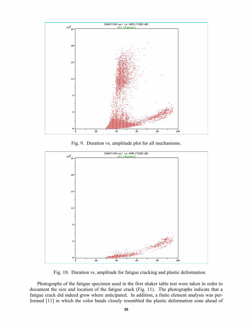
Fig. 9. Duration vs. amplitude plot for all mechanisms.

Fig. 10. Duration vs. amplitude for fatigue cracking and plastic deformation.

Photographs of the fatigue specimen used in the first shaker table test were taken in order to document the size and location of the fatigue crack (Fig. 11). The photographs indicate that a fatigue crack did indeed grow where anticipated. In addition, a finite element analysis was per-formed [11] in which the color bands closely resembled the plastic deformation zone ahead of

31

the crack tip. The plastic deformation zone is somewhat difficult to discern from the photograph of Fig. 11; however, its presence along with the presence of the crack reinforces the validity of the classification process.

(a) (b)

Fig. 11. Fatigue crack, before (a) and after (b) formation.

The above techniques were used to classify the signals received by the AE transducers in the laboratory tests. Reference [11] gives all of the details for each of the laboratory tests, plus ex-plaining the steps required to sort, train, test, and classify AE signals as fatigue cracking, plastic deformation, or mechanical noise. (This includes the correlation of data taken at the two differ-ent threshold values, 10 dB and 30 dB.) The correctly classified signals were subsequently used to train a neural network. The neural network was trained using the data recorded during the laboratory tests. The training file was made up of 300 signals. Of these 300 signals, there were equal numbers of cracking, plastic deformation, and mechanical noise -- 100 of each. These signals were gathered randomly with respect to time.

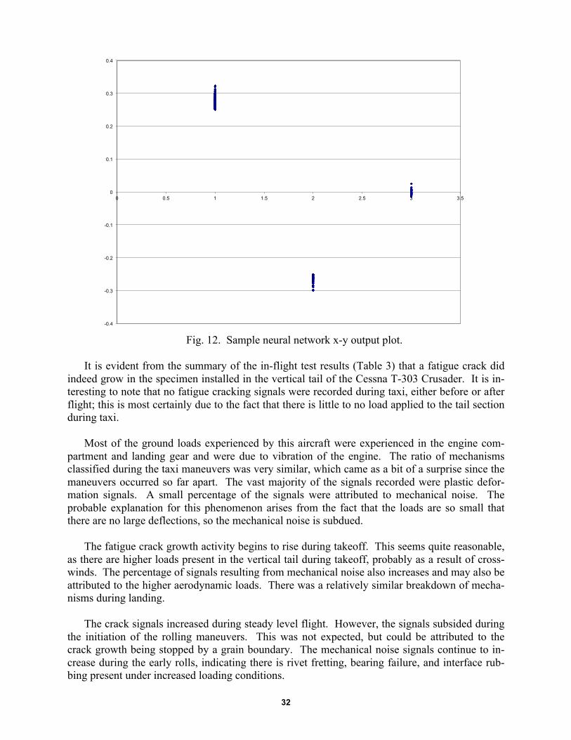
Once the neural network had been trained, it was possible to test the in-flight data by passing it through the trained network. All 15 in-flight data files were tested one at a time. The output of the neural network using the test data was graphed to provide a visual representation of the clas-sified mechanisms (Fig. 12). The output file contains three distinct regions, representing the three failure mechanisms. The first mechanism, fatigue cracking, is seen at the location x = 1 and y ≥ +0.212. The second mechanism, plastic deformation (PD), can be seen at x = 3 and –0.212 < y < +0.212. Finally, the third mechanism, mechanical noise (MN), is at x = 2 and y ≤ –0.212. The values on the x-y plane are the output values of the neural network and can perhaps be represented most simply by the y ranges given in Table 2.

Table 2. Neural network x-y output.

Mechanism Neural Network Output

Fatigue Cracking y ≥ +0.212Plastic Deformation -0.212 < y < +0.212Mechanical Noise y ≤ -0.212

Crack

32

Fig. 12. Sample neural network x-y output plot.

It is evident from the summary of the in-flight test results (Table 3) that a fatigue crack did indeed grow in the specimen installed in the vertical tail of the Cessna T-303 Crusader. It is in-teresting to note that no fatigue cracking signals were recorded during taxi, either before or after flight; this is most certainly due to the fact that there is little to no load applied to the tail section during taxi. Most of the ground loads experienced by this aircraft were experienced in the engine com-partment and landing gear and were due to vibration of the engine. The ratio of mechanisms classified during the taxi maneuvers was very similar, which came as a bit of a surprise since the maneuvers occurred so far apart. The vast majority of the signals recorded were plastic defor-mation signals. A small percentage of the signals were attributed to mechanical noise. The probable explanation for this phenomenon arises from the fact that the loads are so small that there are no large deflections, so the mechanical noise is subdued. The fatigue crack growth activity begins to rise during takeoff. This seems quite reasonable, as there are higher loads present in the vertical tail during takeoff, probably as a result of cross-winds. The percentage of signals resulting from mechanical noise also increases and may also be attributed to the higher aerodynamic loads. There was a relatively similar breakdown of mecha-nisms during landing. The crack signals increased during steady level flight. However, the signals subsided during the initiation of the rolling maneuvers. This was not expected, but could be attributed to the crack growth being stopped by a grain boundary. The mechanical noise signals continue to in-crease during the early rolls, indicating there is rivet fretting, bearing failure, and interface rub-bing present under increased loading conditions.

-0.4

-0.3

-0.2

-0.1

0

0.1

0.2

0.3

0.4

0 0.5 1 1.5 2 2.5 3 3.5

33

Table 3. Summary of In-Flight Results.

Maneuver Crack Events Crack % PD Events PD % MN Events MN %Taxi 0 0.0% 963 93.0% 73 7.0%

Takeoff 69 14.4% 250 52.3% 159 33.3%Flight 277 23.3% 515 43.3% 398 33.4%Flight 1 0.1% 782 66.1% 400 33.8%Flight 7 3.5% 104 52.5% 87 43.9%

Dutch Roll 10 3.9% 113 44.5% 131 51.6%Roll 40 5.1% 383 48.7% 364 46.3%Roll 212 71.9% 52 17.6% 31 10.5%

Dutch Roll 204 73.9% 42 15.2% 30 10.9%Flight 472 64.1% 160 21.7% 104 14.1%

Landing 11 2.3% 331 69.0% 138 28.8%Taxi 0 0.0% 895 93.7% 60 6.3%

During the second roll, the fatigue crack activity began to increase at a rapid rate, peaking during the final Dutch roll. The Dutch roll is a wig-wag maneuver that imposes tremendous aer-odynamic loads on the aircraft, especially the vertical tail. These increased loads were the main reason that the crack activity increased at such a high rate. This higher rate of crack activity was accompanied by a reduction in the presence of mechanical noise as well as plastic deformation. Returning to steady, level flight led to a reduction in the crack signals, followed by landing, where the fall-off continued. Conclusions The goal of this research was to develop an aircraft structural health monitoring system for keeping track of fatigue crack growth while in flight. It has been shown that it is indeed possible to monitor fatigue crack signals in a noisy in-flight environment using AE nondestructive testing techniques in combination with neural networks. In conclusion, this research successfully demonstrated a prototype in-flight AE fatigue crack monitoring system for aircraft structures. It is envisioned that the application of such structural health monitoring systems in aging aircraft could warn of impending failure and allow for replacement of parts when needed rather than at conservatively calculated intervals. Recommendations The next step in the development would be to incorporate the current research being done in back-propagation neural network (BPNN) fatigue life prediction such that it can be applied to the data gathered by in-flight aircraft structural health monitoring systems. Reasonably accurate BPNN fatigue life predictions have been obtained in aerospace bellows [14], notched tensile fa-tigue specimens [15-16], and bridge steel I-beams [17]. In each case, the entire acoustic AE am-plitude distribution for various ranges in the fatigue cyclic life (0-25%, 25-50%, and 50-75%) was input to a BPNN, and the associated fatigue life predictions were made with worst case er-rors of between 5-20% for the three different structures.

34

Analogous work has been done for low proof load (≤25% Pburst) burst pressure predictions in composite pressure vessels in which ±5% worst case errors have been obtained by using the ma-trix cracking only (since matrix cracking is a precursor to delamination and fiber breaks) portion of the AE amplitude distribution as input to the BPNN [18]. Hence, for the fatigue life predic-tion problem, it is recommended that the plastic deformation only data portion of the AE ampli-tude distribution be used as input to a BPNN (since plastic deformation is a precursor to both plane strain and plane stress fatigue crack growth), which should reduce the worst case error pre-dictions to a similar ±5% range. Such prediction accuracies would lead to minimized mainte-nance costs and extended service lives of aging aircraft, which is the ultimate goal of this re-search effort. Acknowledgements

The authors would like to extend a special thanks to fellow graduate student Mr. Samuel G. Vaughn III, whose help in conducting experiments and analyzing data increased the quality of this research. Master of Science in Aerospace Engineering thesis committee members Dr. James G. Ladesic, who contributed by acting as the FAA Designated Engineering Representative (DER) in making modifications to the airplane, and Dr. Frank J. Radosta for his guidance in the finite element analysis of the channel beam structure, must also be thanked. Finally, this materi-al was based upon original work performed by graduate student Mr. Robert J. Demeski and sup-ported by the National Science Foundation Grant # DMI-9503017 under an Embry-Riddle Aero-nautical University (Daytona Beach, Florida) subcontract to Martingale Research Corporation and Principal Investigator Mr. Harvey L. Bodine (now with Neuralytics, Richardson, TX). References 1. Cotta, R. and Levy, L. “Fail Safe Insurance for KC-135.” Aviation. October 1979. pp. 14-

15. 2. Parrish, B. “Acoustic Emission Techniques for In-Flight Structural Monitoring.” SAE

Technical Paper No. 801211. Society of Automotive Engineers, Warrendale, PA, 1980. pp. 1-4.

3. McBride, S.L. and Maclachlan, J.W. “Acoustic Emission Monitoring of Aircraft Structures.” Journal of Acoustic Emission. Vol. 4, April 1985. pp. 151-154.

4. Scala, C.M., Bowles, S.J. and Scott, L.G. “The Development of Acoustic Emission for Structural Integrity Monitoring of Aircraft.” Defense Technical Information Center Acces-sion No. ADA196264. Aeronautical Research Labs, Melbourne, Australia, 1988. pp. 1-35.

5. Granata, D.M., Kulowitch, P. and Scott, W.R. “In-Flight Acoustic Emission Monitoring of Crack Growth.” Review of Progress in Quantitative Nondestructive Testing: Vol. 13A. Edi-tors D.O. Thompson and D.E. Chementi. Plenum Press, 1994. pp. 461-468.

6. Pollock, A.A. "Acoustic Emission Inspection." Metals Handbook. Ninth Edition, Vol. 17, 1989. pp. 278-292.

7. Hill, E.v.K. and Vaughn III, S.G., “Fatigue Crack Monitoring of an Aircraft Engine Cowling in Flight,” Nondestructive Testing Handbook, Third Edition: Volume 6, Acoustic Emission Testing, American Society for Nondestructive Testing, Columbus, OH, 2005, pp. 367-376.

8. Spanner, J.C., Sr. "Acoustic Emission Noise." Nondestructive Testing Handbook (3rd ed.): Vol. 6, Acoustic Emission Testing. Technical Editors R.K. Miller and E.v.K. Hill. Editor P.O. Moore. Columbus, OH: American Society for Nondestructive Testing, 2005. pp. 41-44.

35

9. Fausett, L.V. Fundamentals of Neural Networks. Englewood Cliffs, NJ: Prentice-Hall, 1994. pp. 5-7, 169-175.

10. "Aluminum Reynolds 7075b Uns_A97075 75f Temper_T6 - Aircraft Structure." Cen-BASE/Materials, www.Online.Internet. 1995.

11. Rovik, C.L. “Classification of In-Flight Fatigue Cracks in Aircraft Structures Using Acoustic Emission and Neural Networks.” Master of Science in Aerospace Engineering Thesis. Em-bry-Riddle Aeronautical University, Daytona Beach, FL, 1998.

12. Egle, D.M. "Wave Propagation." Nondestructive Testing Handbook (3rd Edition): Vol. 6, Acoustic Emission Testing. Technical Editors R.K. Miller and E.v.K. Hill. Editor P.O. Moore. Columbus, OH: American Society for Nondestructive Testing, 2005. pp. 96-97.

13. Miller, R.K. "Fundamentals of Acoustic Emission Source Location." Nondestructive Test-ing Handbook (3rd Edition): Vol. 6, Acoustic Emission Testing. Technical Editors R.K. Mil-ler and E.v.K. Hill. Editor P.O. Moore. Columbus, OH: American Society for Nondestruc-tive Testing, 2005. pp. 126-127.

14. Ballard, D.L.W. and Hill, E.v.K. “Fatigue Life Prediction of Edge-Welded Metal Bellows using Neural Networks and Acoustic Emission Amplitude Data.” ASNT Fall Conference and Quality Test Show Paper Summaries. Columbus, OH: American Society for Nondestructive Testing, 1998. pp. 146-149.

15. Suleman, J., Hill, E.v.K., Villa, E. and Okur, M.A. “Neural Network Fatigue Life Prediction in Aluminum from Acoustic Emission Data.” Aging Aircraft 2009, The 12th Annual Joint AIAA/ASME/DoD/NASA Conference on Aging Aircraft, Kansas City, MO, May 2009. 29 pages.

16. Barsoum, F.F., Suleman, J., Korcak, A. and Hill, E.v.K. “Acoustic Emission Monitoring and Fatigue Life Prediction in Axially Loaded Notched Steel Specimens.” Journal of Acoustic Emission.” Vol. 27, 2009. pp 40-52.

17. Barsoum, F.F., Hill, E.v.K., Suleman, J., Korcak, A. and Zhang, Y. “Neural Network Fa-tigue Life Prediction in Notched Bridge Steel I-Beams from Acoustic Emission Amplitude Data.” Journal of Acoustic Emission. Vol. 29, 2011. pp. 251-259.

18. Hill, E.v.K., Iizuka, J., Kaba, I.K., Surber (now McCann), H.L. and Poon, Y.P. “Neural Network Burst Pressure Prediction in Composite Overwrapped Pressure Vessels Using Mathematically Modeled Acoustic Emission Failure Mechanism Data.” Research in Nonde-structive Evaluation, Vol. 23, 2012. pp. 89-103.


Acoustic Emission Monitoring of Composite Blade of NM48/750 NEG-MICON Wind Turbine

Dimitrios Papasalouros1, Nikolaos Tsopelas1, Athanasios Anastasopoulos1,

Dimitrios Kourousis1, Denja J. Lekou2 and Fragiskos Mouzakis2 1Mistras Group Hellas ABEE, El. Venizelou 7 & Delfon, 14452 Metamorphosis, Athens, Greece 2Centre for Renewable Energy Sources and Saving (CRES), 19th km Marathonos Avenue, 19009

Pikermi, Greece,

Abstract In-service monitoring of wind-turbine (W/T) blades during operation presents practical diffi-culties due to accessibility restrictions, nature of the material, size and geometry of the blades as well as power requirements. As a result, attempts for health monitoring of wind turbine blades are limited. In the present paper, health monitoring of the blades of an operating NEG-MICON NM48/750 with acoustic emission (AE) will be discussed. Included are W/T instrumentation and various other technical apparatus that was applied in order to overcome power limitations, re-mote monitoring set up, as well as development of software for automated statistical processing of AE data. The AE module was successfully operated and acquired data, under real operating conditions for more than six months. Results are presented from AE measurements acquired un-der different operating conditions, correlated with parametric data and analyzed with both linear location and advanced AE data processing techniques. Finally the paper discusses the system performance during its total installation time and operating conditions, demonstrating the fast integration into existing structures and its modularity to external systems and data exchange, making it a good candidate for real-time monitoring of industrial size wind generators. Keywords: Wind turbine blades, composite materials, health monitoring, automated AE data processing 1. Introduction Until recently, in-service monitoring of wind turbine blades has not received major attention due to many practical difficulties encountered, such as accessibility restrictions, nature of the material, size and geometry of the blades as well as power requirements. However, given the in-creased size of modern wind turbine (W/T) blades of lengths up to 75m on the latest wind gener-ators and their growing complexity and fabrication cost, blade monitoring is becoming more and more important to operators, since maintenance is difficult and the potential financial losses ac-cruing from unscheduled outages are increasingly growing, especially when off-shore W/T are concerned, where replacing a damaged blade is a major undertaking. In-service monitoring could detect structural degradation long before ultimate blade failure, and would allow the operator to decide whether a preventive maintenance should occur as soon as possible or whether the blade should be left turning until the next scheduled maintenance period.

Acoustic emission (AE) is highly effective in detecting and identifying damage in W/T blades and generally composites under load, and has proven its validity through numerous labor-atory tests including full-scale blade tests [1-7]. However, in-service monitoring experience of W/T blades was limited [8] until recently when a NEG-MICON NM48/750 W/T of Center for Renewable Energy Sources and Saving (CRES) wind farm was instrumented with a multichannel AE system for structural health monitoring of the W/T blades during operation [9-11]. The

37

system was successfully installed and operated for more than 6 months under real operating con-ditions, collecting a considerable amount of AE data, enabling evaluation of the system under different operating conditions.

In the present paper results from AE measurements acquired under different operating condi-

tions, correlated with parametric data and analyzed with both linear location and advanced data processing techniques will be presented. In addition, presentation includes W/T instrumentation and various other technical apparatus that was applied in order to overcome power limitations, as well as remote monitoring set up and development of software for automated statistical pro-cessing of AE data. Finally the paper discusses the system performance during its total installa-tion time and operating conditions, demonstrating the fast integration into existing structures and its modularity for connection to external systems and data exchange, making it a good candidate for real time monitoring of industrial size wind generators. 2. Instrumentation of an In-service Wind Turbine AE monitoring of W/T blades during operation poses several challenges and difficulties to be met by the condition monitoring system, not only due to the (inherent in composites) complex nature of the blade’s defects aimed to be detected, but also for a number of application-specific factors such as:

• the harsh environment and the conditions under which such a system will operate, • accessibility reasons for system installation in the hub and sensor mounting (e.g. on the

inside surface of the blades), • power issues for the system residing in the hub, and, most important, • the necessity for wireless data communication or telemetry posed by the rotation of the

blades. In addition, since AE may often be correlated to or caused by external parameters such as rota-tional speed, wind, loading, manipulations etc., the AE Condition Monitoring System (CMS) should be capable of real-time acquisition of such parameters, in order to enhance analysis and interpretation.

The AE CMS selected for this project meets the above requirements as it is a compact, multi-channel AE system (Micro-II by Physical Acoustics Corporation (PAC)), with low power con-sumption (below 100W) and versatile to be powered by dc input (occasionally available in the nacelle of mid-sized turbines – as opposed to standard 220Vac), relatively light weight in order to be quickly mounted on rotating parts and to minimize unbalancing forces due to its incorpora-tion inside the hub, and also having the capability of being remotely controlled as well as trans-mit the collected data through a wireless network (Fig. 1a). In addition, it can be loaded with up to 4 multi-channel AE boards (Fig. 1b), providing up to 32 active AE channels. Finally, for the purpose of enhanced data interpretation and correlation with test and loading conditions, it ac-cepts external signals such as wind velocity, rotation speed, torque, yaw angle, etc. from existing wind turbine instrumentation.

The AE sensors used were three PAC-R6I-AST with resonant frequency of 60 kHz and five PAC-R15I-AST with resonant frequency of 150 kHz. Both types of sensors incorporate integral amplifier allowing them to drive long cables without the need for a separate preamplifier and al-so minimize the RFI/EMI interference. In addition, they feature an Auto Sensor Test (AST) ca-pability allowing the sensors to act as pulsers and remaining as receivers simultaneously, ena-bling automated verification of each sensor coupling and performance at any time desired by the

38

user. AE sensors’ mounting was performed on the inner surface of one of the three blades (with the blades on the wind turbine) using special hold-down devices developed by CRES for the long term attachment of the sensors while sensor cables were connected and securely routed to the rotor’s hub.

(a)

(b) Fig. 1. (a) PAC Micro-II AE system installation inside the hub and (b) PCI-8 AE board.

Fig. 2. Schematic illustration of the structural condition monitoring AE system.

Using the eight AE sensors mentioned above, three different linear groups were considered, in

order to monitor three different areas of the blade. The first group, consisting of sensors (R15I-AST) corresponding to channels 1 and 2, was used to monitor the AE activity on the internal spar of the blade. The second sensor group, consisting of channel 3 to channel 5 (R15I-AST), was used to monitor the AE activity on the trailing side of the blade. Finally the third group, consist-ing of sensors corresponding to channels 6 to 8 (R6I-AST), was used to monitor the AE activity on the root. Sensor placement along the blade, as well as an illustration of the complete structural AE CMS, is shown in Fig. 2, while sample images of the sensors mounted using the specially developed hold-down fixtures are shown in Fig. 3 and Fig. 4.

VIA WIFI CONNECTION / VIRTUAL DESKTOP AT

CLOSE PROXIMITY

VIRTUAL DESKTOP ON REMOTE LOCATION TERMINALS / PERIODIC STATISTICS TO SCADA

1.22 m

0.5 m

0.75 m

0.75 m

1.0 m

PAC SAMOS MICRO II

WIRELESS ROUTER

CH6

CH7

CH8

STRAIN GAUGE

CH5

CH4 CH2

CH3 CH1

Max Strain

Position Min Strain

Position

39

(a) (b) Fig. 3. (a) Mounting of two AE sensors on the internal spar of the blade and (b) one of the three AE sensors mounted on the inner surface of the trailing side of the blade

(a) (b) Fig. 4. One of the two AE sensors mounted on the internal spar of the blade and (b) one of the three AE sensors mounted near blade’s root.

The system was powered with 12V dc through a slip-ring installed on the main shaft of the wind turbine by CRES personnel (Fig. 5a), since there was no power available inside the hub of the stall control wind turbine. However, this slip-ring is not needed on latest wind turbines since most of them provide power inside the hub. Finally, a strain gauge bridge for monitoring edge-wise bending moments was mounted on the outer surface of the blade and was connected to the parametric interface of the AE system (Fig. 5b). This would allow the exact information about the blades’ position during AE activity to be recorded, as well as an approximate estimation of the power output, enhancing the analysis of the AE data acquired by the system.

3. System Connection to SCADA

The AE CMS was connected through wireless connection provided by a wireless router posi-tioned in the base of the W/T tower to the Ethernet network available on the wind turbine and, through this, to the Internet. This way the system could be monitored from anyplace with internet access and it could also transmit the complete AE data acquired and/or only statistical data and alarms to the central monitoring system of the wind turbine. In addition, the AE system was able to send automated emails notifying about detected faults, exceeding thresholds or normal opera-tion of the system (Fig. 6a). A system upgrade could also enable notifications and alerts to be sent automatically through SMS.

(a)

40

(a) (b) Fig. 5. (a) Installation of the slip ring to supply power to the AE CMS. (b) Mounting of a strain gauge on the outer surface of the leading edge of the blade

In addition, through special software developed (Fig. 6b), the system was able to process in real-time the recorded AE data and automatically produce periodical statistics for all the time-driven (TDD) and hit-driven (HDD) data features, which were then sent over the wireless net-work to the central monitoring server.

(a) (b)

Fig. 6. (a) Setup of internet monitoring and automated email notifications. (b) Software interface setup for performing automated AE statistical processing. 4. AE Setup & Location of Simulated AE Sources & Events

In order to estimate the AE generated from the different monitored parts of the W/T blade the mounted sensors were grouped through the acquisition software in three separate linear location groups, as noted in Sec. 2. After sensor installation several tests were performed within the linear segments that were defined from the sensor topology. For these tests, Hsu-Nielsen (HN) sources [14] were applied between all sensor pairs and real time linear location capabilities of the acqui-sition software were verified. Figure 7 shows the results of the X position of the linear event lo-cation between sensors corresponding to channels 1 and 2 that define the monitoring area of the

41

spar, during introduction of artificial AE sources along the sensor line. Additionally, Fig. 8 shows located AE events at the monitoring area of trailing edge of the blade, within the linear span defined by channels 3 to 5. In both Figs. 7 and 8, attenuation in dB/m can be also estimated from the Amplitude (dBae) drop versus X position (m).

Fig. 7. Amplitude vs. Event Location (x - marks) and (#) Hits vs. X Event Location (Bars) for AE located HN source applied in spar area showing located events.

Fig. 8. Amplitude vs. Event Location (x - marks) and (#) Hits vs. X Event Location (Bars) for AE located HN source applied in trailing edge area. Color for channel of first hit. Red: Ch. 3, Green: Ch. 4, Blue: Ch. 5.

Overall, the location of simulated AE events has yielded accurate results, thus providing high

confidence that, if damage occurs and starts accumulating under operating conditions, the system will have the sensitivity to locate it within the monitored areas. Additional real-time location alarms can be set up from the system as output triggers in order to provide extra monitoring in-puts to any given central monitoring system. 5. Continuous Monitoring

System was successfully installed and operated via the connected networks. In total, more than six months of data under real time conditions were acquired. Statistically, this time period is long enough to capture a large variation of the W/T operating parameters and conditions, which may have different impact upon the AE of the inspected area. The AE module acquired more than 300 GB of data during its continuous operation. The system performance and operation were checked randomly during its total operating time, by different experienced AE operators, in different times from different local and international terminal locations in order to provide feed-back for its usability and performance. On-line data analysis was performed using the advanced AE analysis software NOESIS [13] installed in the same system, while the system was in data acquisition mode. The system’s behavior was found to be very reliable and stable in all cases,

Channel 2

Channel 1

42

even during prolonged periods of power loss or technical difficulties, in which cases the system always rebooted and resumed operation and acquisition when the power was restored. A presen-tation of the wind speed, generated power and wind direction variation during the last two months of system operation is shown in Fig. 9.

Fig. 9. Wind speed (m/sec), Average Generated Power (kW) of NEG – MICON 750 and Wind Direction (degrees) vs. Time (days) from October 13th to December 21st 2011 (69 days of 10 min statistical data from CRES). The color ranges of the data correspond to the average RPM of the wind turbine (0-22 RPM).

The additional color dimension in Fig. 9 represents the 10 minutes average rotational speed of the wind turbine rotor. The zero RPM values are colored green in order to show the periods that the generator was stopped either from a lack of wind, maintenance or other reasons. The blue color represents the low RPM operation (15 RPM) as well as any intermediate values that the generator RPM increases from zero to low RPM or low to high RPM (22 RPM). Finally the red color was used in order to identify the periods that the generation was operating in high RPM. It is worth noting that even when the generator was at stop position there is still AE from the blade due to the wind loading indicating the stochastic nature of loading and thus of the AE data. In addition, the distribution of Average Signal level (dB) in correlation with parametric values (Figs. 10 and 11) also highlights the stochastic nature of the data set. The attempt for a simplified analysis based on Time Driven Data alone did not result in information that can be connected with incipient damage.

6. AE Data Analysis

As previously mentioned, a simple review of Figs. 9, 10 and 11 should reveal the stochastic nature of loading and the weather operating conditions that the wind turbine was subjected to during the monitoring period. In order to overcome the limitations imposed from the simplified Time Driven data analysis, the complete AE data set was acquired and processed. During the to-tal time that the system was in acquisition, while installed inside the hub of the wind generator, the volume of acquired data exceeded 300 GB. This six-month period should be statistically suf-ficient to encapsulate the generated AE from the majority if not all the operating and loading conditions. This results in a unique and complete set of AE data that should reflect an actual op-eration of the wind turbine in larger installations.

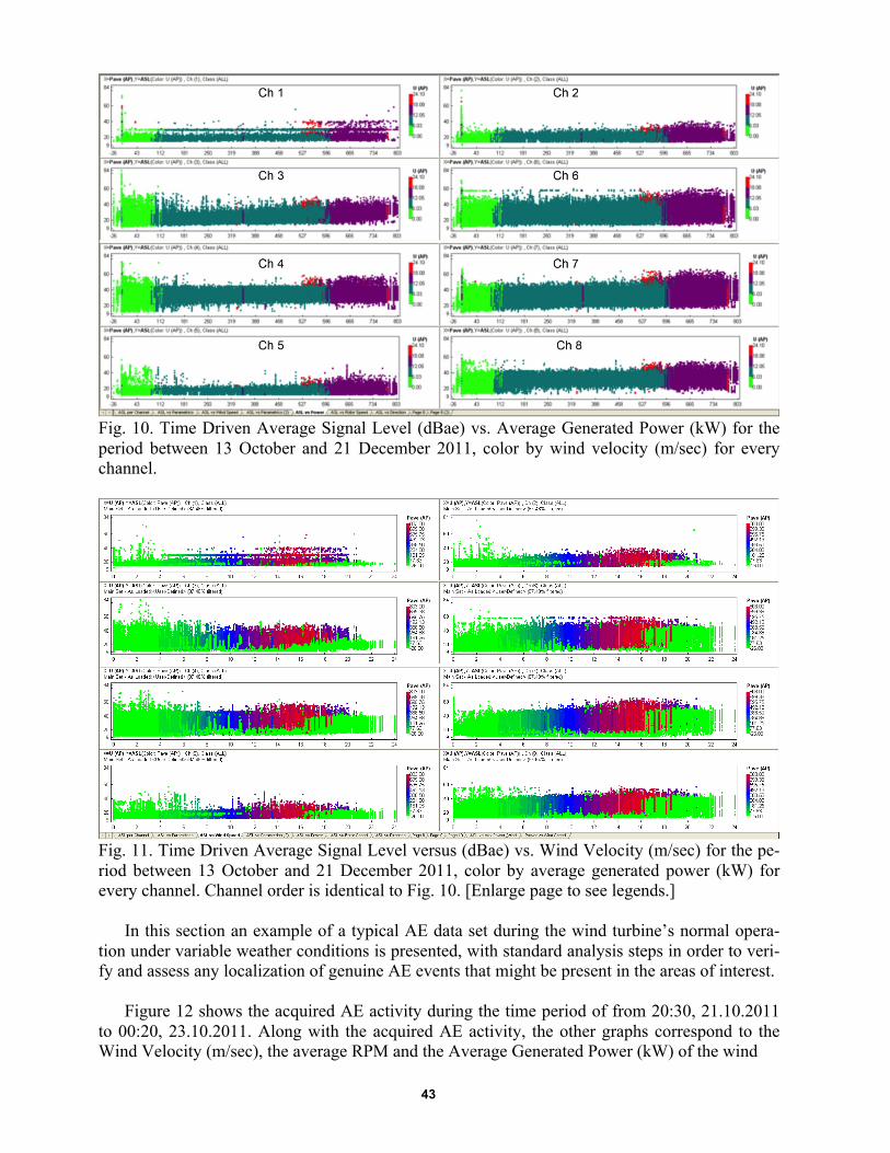
43

Fig. 10. Time Driven Average Signal Level (dBae) vs. Average Generated Power (kW) for the period between 13 October and 21 December 2011, color by wind velocity (m/sec) for every channel.

Fig. 11. Time Driven Average Signal Level versus (dBae) vs. Wind Velocity (m/sec) for the pe-riod between 13 October and 21 December 2011, color by average generated power (kW) for every channel. Channel order is identical to Fig. 10. [Enlarge page to see legends.]

In this section an example of a typical AE data set during the wind turbine’s normal opera-tion under variable weather conditions is presented, with standard analysis steps in order to veri-fy and assess any localization of genuine AE events that might be present in the areas of interest.

Figure 12 shows the acquired AE activity during the time period of from 20:30, 21.10.2011

to 00:20, 23.10.2011. Along with the acquired AE activity, the other graphs correspond to the Wind Velocity (m/sec), the average RPM and the Average Generated Power (kW) of the wind

44

turbine. The wind velocity, average RPM and generated power data were provided by CRES and correspond to average values over a 10-minute time period.

Fig. 12. From top to bottom: AE amplitude (dB) vs. time (sec), wind velocity (m/sec) vs. time (sec), rotational speed (RPM) vs. time (sec) & average power output (kW) vs. time (sec).

Fig. 13. First Hits of Located Events vs Time (sec). From top to bottom: Group of Channels 1-2 (Spar Area), Group 2 of Channels 3-5 (Trailing Edge Area), Group 3 Channels 6-8 (Root Area). The specific data set was selected in order to investigate and assess the generated AE, caused by the variable operating conditions. In the presented time segment, the wind generator goes from a complete stop to normal operation due to rising wind velocity. Periods of low RPM and high RPM are also visible along with the specific times that the rotational speed was changed from low to high. Additionally, the wind throughout the selected time span appears to have sig-nificant variations and the resulting AE activity especially during the last hour of the time

45

segment (specifically, 31 to 100 ks) is of interest due to the fact that an increasing trend is visible in AE activity while the wind velocity significantly drops and then rises up again. Figure 13 shows the located events per sensor group during the time segment under investigation. Linear location for each sensor group of the raw data of the specific time segment is performed and graphs of the located first hits of the monitored areas are generated (Fig. 14). The first hits of the located AE events from each monitored area (Spar, trailing edge & root) were easily separated using NOESIS [13] for their features to be compared with the simulated HN sources that were applied on the same monitored area. An X position distribution of the located AE events (first hits) from each monitored area is shown in Fig. 14.

Fig. 14. First Hits of Located Events vs. Event’s X Location (m). From top to bottom: Group of Channels 1-2 (Spar Area), Group 2 of Channels 3-5 (Trailing Edge Area), Group 3 Channels 6-8 (Root Area).

The following graphs (Fig. 15) show in blue the first hits of the located AE events on the monitored area of the spar during the 24 hour segment under analysis. Overlaped in red is the dataset of first hits of simulated HN sources. The red dataset (simulated sources) corresponds to the expected AE events that should be present in the case of actual damage in this monitored area. Direct comparison of both data sets reveals that the acquired data clusters have a good separation. The signatures obtained due to the stochastic wind loading and the estimated feature characteristics that correspond to HN sources show that an qualitative AE signal estimation can be made seperating the signals from the general wind loading and operation of the wind turbine with those corresponding to incipient damage.

By reviewing these graphs useful conclusions can be drawn. The located AE events when

compared with the simulated sources applied on the same areas appear to have similar durations and counts but an amplitude range lower and close to the low sensitivity limit of the system. The large volume of AE that is acquired by the equipment corresponds to many different phenomena during the operation of the wind turbine. For the specific case, only sources that have similar AE features to the simulated ones are of interest. In the specific area, a small amount of AE activity (~5 events out of more that 400,000 AE hits) can be considered relevant. Due to the fact that this activity corresponds to a full data set of approximately 24h, it can be also considered a very low AE activity. The aforementioned facts yield an approximation of the AE rates, amplitudes and features ranges that are to be expected during normal operation. These can be used to fine-tune

46

the AE system for minimal data acquisition (and therefore data volume efficiency) focused in the desired and expected parameters.

Fig. 15. Signature graphs of AE features (in 2D & 3D feature space), in blue are the located AE events in the spar area during the 24h time segment under analysis and in red the simulated HN sources. Circled Xs mark 5 relevant located AE events. Some outlier hits in red are also marked. [These markings become clearly visible by expanding this figure to 500%. Also see arrows.]

Fig. 16. Signature graphs of AE features (in 2D & 3D feature space), in blue are the located AE events in the trailing edge area during the 24h time segment under analysis and in red the simu-lated HN sources.

The same analysis is performed for the remaining two monitored areas of the trailing edge and the root section of the blade of the wind turbine. Figure 16 shows in blue the first hits of the located AE events on the monitored area of the trailing edge during the 24h segment under analysis. Overlaped in red is the dataset of first hits of simulated HN sources applied on the same area. The red dataset (simulated sources) corresponds to the expected AE events that could be present in the case of incipient damage in this monitored area. As in the previous case, good

47

cluster separation appears to exist using both two-dimensional and three-dimensional feature co-ordinates.

In the final case of the third monitored areas (root area), the clusters separation between nor-

mal turbine operation and simulated HN sources again appears to be good and to yield clear dis-tinction between the two feature areas of interest. Figure 17 shows in blue the 24h data from normal turbine operation and in red the HN simulated sources applied on the same area. As in all previous cases, these signatures can be used to fine-tune the system to acquire only the AE data of interest that should correspond to incipient damage.

Fig. 17. Signature graphs of AE features (in 2D & 3D feature space), in blue are the located AE events in the root area during the 24h time segment under analysis and in red the simulated HN sources. Selection of 191 relevant located AE events is shown. Additionally there is a clear clus-ter separation in 3d feature space 7. Conclusions Based on the large continuous monitoring period and the selected analysis period, the AE signa-tures of the normal operation of the wind turbine are obtained. Based on this large statistical AE data set and the AE signatures obtained from the simulated HN sources, a direct comparison is enabled on the corresponding monitored areas. This comparison can be used in order to maxim-ize the efficiency of continuous monitoring in various respects. One example is that the ranges of the estimated normal operation signatures based on multiple features can be set as alarm and/or front end filters. In this way the system is mainly focused to features space areas that have a higher likelihood to correlate with incipient damage while discarding all other (irrelevant) data, ensuring a more compact data set, thus greatly minimizing the data storage needs. In addition, due to the more compact data set, streaming of data will be more efficient as well.

The AE signatures of the normal operation of the wind turbine blade are estimated in this

case using representative 24h data. This data set was selected due to the fact that on the specific times all the different cases of variable wind velocity coexist. Therefore this can be considered as the limit case data since the wind turbine goes from a complete stop to low and high RPM and there is a significant wind velocity variation between low and high values. The previous figure shows the different AE signatures from located AE data from the monitored areas of the blade in

48

blue. In red, the HN simulated sources signatures are overlapped in order to enable an overall comparison between the signatures of the different areas. It appears that the AE signature for each area has a different and rather unique 2D cluster shape (Fig. 18).

Fig. 18. Signature graphs of AE features (in 2D feature space), in blue are the located AE events and in red the simulated HN sources. From left to right columns are the signatures of the spar, trailing edge and root area.

Finally, from the analysis of a selected part of a large AE data volume, acquired from a per-manently installed AE monitoring system on an operating wind turbine blade, promising results were observed, based on the direct comparison and dissimilarities between simulated sources and located AE signal signatures on the monitored areas. The comparison is established on the basis of the degree of dissimilarity between three standard AE features. The correlation of these fea-tures usually provides an initial estimation about the origin of AE caused by different phenome-na. The observations made can also be used for fine-tuning the real time response triggers of the system by setting up front end filters to issue alarms to any connected monitoring system. Addi-tionally, the endurance and modularity of newer AE acquisition systems was successfully demonstrated during actual daily operating conditions in the health monitoring of the NEG-MICON NM48/750 blade. Future work includes the demonstration and modularity of the system with other types of wind generators, as well as other real time analysis capabilities or during post processing by using modern AE software suites.

Long-term acquisition until actual damage on the blade is developed and verified will enable evaluation of system’s capability for real-time early damage identification and warning. The same may be, alternatively, achieved through installation of the system in already verified but non-critically damaged blades (preferably similar to the ones already monitored). Acknowledgements The research leading to these results has received funding from the European Community’s Sev-enth Framework Programme (FP7/2009-2013) under grant agreement no 239462.

49

References 1. Sutherland, H., Beattie, A., Hansche, B. et al. 1994. The Application of Non-Destructive

Techniques to the Testing of a Wind Turbine Blade, Sandia National Laboratories report, Ref: SAND93-1380.UC-261, New Mexico, U.S.A.

2. Anastasopoulos, A.A., Kourousis, D.A., Vionis P. and Kolovos, V. 1999. Acoustic Emission NDE of a Wind Turbine Blade during full scale testing. INSIGHT, Vol. 41, No 6.

3. Vionis, P.S., Anastasopoulos, A.A., Kolovos, V.K., Kouroussis, D.A., 1999. Non-Destructive Testing of Full Scale W/T Blade by means of Acoustic Emission Monitoring During Controlled Static Loading, Wind Energy for the Next Millennium, Proc. 1999 Euro-pean Wind Energy Conference, Acropolis Convention Centre, Nice, France, pp. 691-694.

4. Kouroussis, D., Anastasopoulos, A., Vionis, P., Kolovos, V. 2000. Unsupervised Pattern Recognition of Acoustic Emission from Full Scale Testing of a Wind Turbine Blade. J. Acoustic Emission, Vol. 18, pp 217-223, ISSN 0730-0050 Coden JACEDO.

5. Kouroussis, D., Anastasopoulos, A., Vionis, P., Kolovos, V. 2000. Acoustic Emission Moni-toring of a 12m Wind Turbine FRP Blade during Static and Fatigue Loading, in “Emerging Technologies in NDT”, Eds. Hemelrijck, D. Van, Anastasopoulos, A. A. and Philippidis, T., Balkema, pp. 59-66.

6. Anastasopoulos, A. A.,Kouroussis, D. A., Nikolaidis, V. N., Proust, A., Dutton, A. G., Blanch, M., Jones, L. E., Vionis, P., Lekou, D. J., Delft, D R V van, Joosse, P. A., Philippi-dis, T. P., Kossivas, T., Fernando, G., 2002. Structural Integrity Evaluation Of Wind Turbine Blades Using Pattern Recognition Analysis On Acoustic Emission Data. J. Acoustic Emis-sion, Vol. 20, pp. 229-237.

7. Lekou, D.J., Vionis, P., Joosse, P.A., Delft, D.R.V. van, Kouroussis, D., Anastasopoulos, A., Blanch, M.J., Dutton, A.G., Proust, A., 2003. Full-Scale Blade Testing Enhanced By Acous-tic Emission Monitoring. EWEC 2003 proceedings, European Wind Energy Conference and Exhibition, Madrid, Spain.

8. Blanch, M.J., Dutton, A.G., 2003. Acoustic Emission Monitoring of Field Tests of an operat-ing Wind Turbine, Damage Assessment of Structures, Proceedings of the 5th International Conference on Damage Assessment of Structures (DAMAS 2003), Southampton, UK.

9. Kourousis, D., Lekou, D., Tsopelas, N., Papasalouros, D., Mouzakis, F., Anastasopoulos, A. 2010. Health Monitoring of Wind Turbine Blades with Acoustic Emission, Proceedings of the 7th Νational Conference of the Hellenic Society of Non-Destructive Testing (HSNT), “The Contribution of Non Destructive Testing for the Safe of Small and Big Works and Con-structions”, NTUA, Athens, Greece.

10. Kourousis, D., Tsopelas, N., Ladis, I., Anastasopoulos, A., Lekou, D.J., Mouzakis, F., 2011. Health Monitoring of Wind Turbine Blades with Acoustic Emission, Proceedings of the Eighth International Conference on Condition Monitoring and Machinery Failure Preven-tion Technologies, BINDT – CM2011 Conference, 20-22 June 2011, Cardiff, UK.

11. Tsopelas, N., Kourousis, D., Ladis, I., Anastasopoulos, A., Lekou, D.J., Mouzakis, F., 2011.Health Monitoring of Operating Wind Turbine Blades with Acoustic Emission, Pro-ceedings of the 5th International Conference on Emerging Technologies in Non Destructive Testing, 19-21 September 2011, UOI, Ioannina, Greece, pp. 347-352.

12. “Development and Demonstration of a Novel Integrated Condition Monitoring System for Wind Turbines – NIMO”, Seventh Framework Programme of the European Community (2007-2013), http://www.nimoproject.eu/

13. NOESIS Ver. 5.2, Envirocoustics, User’s Manual. 14. ASTM E976, Standard Guide for Determining the Reproducibility of Acoustic Emission

Sensor Response.

Journal of Acoustic Emission Volume 31, · PDF fileJournal of Acoustic Emission Volume 31,...

Documents

Transcript of Journal of Acoustic Emission Volume 31, · PDF fileJournal of Acoustic Emission Volume 31,...