NBER WORKING PAPER SERIES

JOINT LIFE ANNUITIES AND ANNUITYDEMAND BY MARRIED COUPLES

Jeffrey R. Brown James M. Poterba

Working Paper 7199http://www.nber.org/papers/w7199

NATIONAL BUREAU OF ECONOMIC RESEARCH1050 Massachusetts Avenue

Cambridge, MA 02138June 1999

We are grateful to Peter Diamond, Michael Hurd, Larry Kotlikoff, Olivia Mitchell, Antonio Rangel, MarkWarshawsky and participants in the NBER Summer Institute on Aging for helpful comments, and to TIAA-CREF, the National Institute on Aging, the Social Security Administration, and the National ScienceFoundation for research support. All opinions expressed are those of the authors and not those of the NationalBureau of Economic Research.

© 1999 by Jeffrey R. Brown and James M. Poterba. All rights reserved. Short sections of text, not to

exceed two paragraphs, may be quoted without explicit permission provided that full credit, including © notice,is given to the source.Joint Life Annuities and Annuity Demand by Married CouplesJeffrey R. Brown and James M. PoterbaNBER Working Paper No. 7199June 1999JEL No. H55, J14

ABSTRACT

This paper explores the value of purchasing joint life annuities for married couples. It describes the

existing market for joint life annuities, and summarizes the range of annuity products that are currently

available to couples. It then considers the value that married couples would place on access to an

actuarially fair annuity market, and defines a measure of willingness-to-pay for annuities. This calculation

differs from the analogous one for a single individual for two reasons. First, joint-and-survivor life tables

differ from individual life tables. The life expectancy of the second-to-die in a married couple is

substantially greater than that for a single individual. Second, joint life annuities provide time-varying

payouts, because survivor benefit options permit the payout when both members of a couple are alive to

differ from that when one member has died. The paper develops a new annuity valuation model and applies

it to evaluate a married couple's utility gain from annuitization. The findings suggest that previous estimates

of the utility gain from annuitization, which applied to individuals, overstate the benefits of annuitization for

married couples. Since most potential annuity buyers are married, these findings may help to explain the

limited size of the private market for single premium annuities.

Jeffrey R. Brown James PoterbaKennedy School of Government Department of EconomicsHarvard University MIT E52-35079 John F. Kennedy St. Cambridge, MA 02139-4307Cambridge, MA 02138 and NBERand NBER poterba@mit.edubrown@nber.org

1

Annuities play an important role in the theory of consumer choice when there is uncertainty

about length of life. Yaari (1965) showed that an individual with a fixed stock of resources and an

uncertain lifetime should purchase an annuity contract to insure against the risk of outliving his resources.

More recent work shows that the gains to annuitization for individual life-cycle consumers can be

substantial. Mitchell, Poterba, Warshawsky, and Brown (1999) find that a typical 65-year old retired

male life cycle consumer would be willing to give up roughly one third of his wealth to gain access to an

actuarially fair nominal annuity market.

A number of studies have observed that despite the apparent benefits of annuitization, the

market for individual annuity contracts in the United States is very small. This has resulted in several

attempts to explain the limited flow of new annuity purchases. One group of empirical studies, including

Friedman and Warshawsky (1988, 1990) and Mitchell, et al. (hereafter MPWB) (1999), have

explored the extent of adverse selection in the individual annuity market. While annuitants are, on

average, significantly longer-lived than individuals in the population at large, the degree of adverse

selection does not seem sufficient to explain the absence of annuity purchases.

A second set of studies, surveyed in Laitner (1997) and Altonji, Hayashi, and Kotlikoff (1997),

have focused on intergenerational altruism as a potential explanation for limited annuity demand. This

work suggests that simple altruistic models do not provide a satisfactory explanation for observed

patterns of intergenerational transfers.

Yet a third group of studies has shown that while individuals rarely purchase annuity contracts, a

substantial fraction of their retirement resources is already annuitized. Auerbach, Kotlikoff, and Weil

(1992) show that when Social Security benefits, private defined benefit pension plan payments, and

Medicare benefits are added together, more than half of the resources of the current elderly in the

United States take the form of life-contingent payouts (annuities). This suggests that one reason

2

individuals do not purchase additional annuities is because they are already substantially annuitized.

The functioning of private annuity markets has recently attracted attention as part of the policy

debate on "individual accounts" alternatives to current pay-as-you-go, defined benefit Social Security

systems. A central policy design issue concerns the way a retiree could spread the resources

accumulated in an individual account over his, or his and his spouse's, remaining lifetime. While the

treatment of married couples is an important issue in Social Security program design, virtually all of the

previous research on annuities has focused on individuals rather than couples as decision-making units.

This paper presents new evidence on the structure of joint-life annuity products that insurers currently

offer, and it evaluates these annuity contracts from the standpoint of couples.

Two previous studies have investigated the post-retirement consumption behavior of married

couples as opposed to individuals. The first, by Kotlikoff and Spivak (1981), focused on the demand

for individual annuities by married rather than single persons. This paper showed that if married

individuals, or more generally those in an extended family, were able to contract to share resources over

their respective lifetimes, then the benefits of purchasing an individual annuity contract were smaller than

those for independent individuals. This result arises from the fact that risk sharing within families is a

partial substitute for risk sharing in an organized annuity market. Kotlikoff and Spivak (1981) did not

consider the demand for joint life annuities by married couples.

A second related study is Hurd’s (1999) investigation of optimal consumption by married

individuals when both members of the couple face uncertainty about length of life. This paper presents

new findings on how couples should structure their consumption in the absence of an annuity market.

Hurd's study shows that optimal consumption depends on the structure of the household utility function,

and it draws attention to the absence of an agreed-upon framework for modeling the joint decisions of

married couples.

3

Modeling difficulties should not obscure the key role that couples rather than single individuals

are likely to play in both public and private annuity markets. In the United States in 1995, 77 percent

of men and 43 percent of women over age 65 were married. Most individuals are members of married

couples at the beginning of their retirement years, the age at which annuity purchase is most likely. Not

surprisingly, given these demographic facts, LIMRA (1997) reports that married persons buy 77

percent of all annuity contracts, and 85 percent of single-premium contracts. Single-life annuity contracts

without any provisions for spouses or survivors are unusual. Period certain and joint-and-survivor

annuity contracts, both of which provide some spousal protection, are much more common.

In this paper, we explore two issues related to married couples' demand for private annuities.

First, we describe the range of joint life annuity products that is currently available. We show that

existing annuity products are much more complex than textbook level-premium, single-life annuities, and

that these products provide married couples with resource allocation options that cannot be achieved

with single-life annuity products alone. Second, we extend previous work on the amount that

individuals, or in our case married couples, would be prepared to pay to obtain access to an actuarially

fair annuity market. We specify a household utility function and explore the increase in household utility

that takes place when a couple is able to participate in an actuarially fair market for joint life annuities.

We then translate this increase in utility into an "annuity equivalent wealth," which is the amount of

additional wealth that a couple would need to be as well off without access to an annuity market as with

such access. This segment of our research extends the dynamic programming analysis of optimal

lifetime consumption in MPWB (1999) and Brown, Mitchell, and Poterba (1999) from an individual to

a couple. By focusing on joint annuity products, we consider a wider menu of annuity payout options

than previous studies.

The paper is divided into four sections. The first describes the structure of currently-available

4

joint annuity products. Section two presents our algorithm for evaluating the utility gains associated with

participating in an actuarially fair joint annuity market. Section three reports our basic results on the

“annuity equivalent wealth,” along with sensitivity tests for the impact of changing assumptions about

mortality rates and the degree of pre-existing annuitization. The fourth section concludes and suggests

several further research issues.

1. The Marketplace for Joint and Survivor Annuity Contracts

To analyze the role of joint life annuity contracts, it is important to recognize that a married

couple is concerned with four distinct states of the world. The first state is that in which both members

of the couple are alive, and income is used to support the consumption of both spouses. The three

other states are one in which the wife is a widow, one in which the husband is a widower, and one in

which both spouses are deceased. A couple that makes rational financial decisions will seek to

optimally allocate wealth across these four states. In the presence of a bequest motive, the couple may

choose to allocate some resources to the state in which both members of the couple are dead. Joint

annuities allow couples to make their income stream contingent on these survival states.

There are two primary types of joint annuity contracts. The first is a joint life annuity with a last

survivor payout rule. This rule specifies a periodic payment, typically monthly or quarterly, that the

annuitants will receive provided both of them are still alive. In addition, it specifies a fraction of this

payment, φ, that will be paid to the survivor after the death of one member of the couple. The fraction

φ is usually set at 1, 2/3, or ½, although LIMRA (1997) reports that insurance companies will provide

virtually any fractional survivor benefit at the request of the annuity buyer. In the special case of φ = 1,

the annuity provides a level payout stream from the time it is purchased until the death of the last

surviving spouse. This is sometimes referred to simply as a “joint and survivor annuity.”

5

To define an actuarially fair joint and survivor annuity with a last survivor provision, let A denote

the fixed nominal benefit that is paid as long as both members of the couple are alive, and let Sm,j denote

the probability that the husband in the annuity-purchasing couple survives for at least j months after

purchasing the annuity. In an analogous fashion, define Sf,j as the j-period survival probability for his

wife. The equation for actuarial fairness of the premium (P) associated with a joint and survivor annuity

contract is:

.iSSSSASSA = P jjfjmjmjfjfjmj=1 )1/())}1(*)1(*(****{ ,,,,,, +−+−+∑∞ φ (1)

We use i to denote the nominal, after-tax interest rate at which the insurance company discounts future

payouts.

The second type of joint life annuity policy is a joint life policy with a contingent survivor benefit.

The key distinction between this type of policy and a last survivor policy is that the contingent benefit

policy specifies one member of the couple as a primary annuitant. Provided the primary annuitant is

alive, the annuity payout is A per period. If the primary annuitant predeceases the secondary annuitant,

however, the payout declines to a fraction θ of the primary annuitant’s payment. If θ = 1 then the

contingent survivor annuity is equivalent to a last survivor annuity with φ = 1, but when θ < 1, the policy

differs from a last survivor policy with φ < 1. With a contingent survivor annuity, the order in which the

two annuitants die matters for the time profile of benefits, and thus the spouses are treated

asymmetrically with regard to the survivor benefit.

The condition that defines an actuarially fair joint life annuity with a contingent survivor benefit,

assuming for purposes of illustration that the husband is the primary annuitant, is:

.iSSASA = P jjfjmjmj=1 )1/(})1({ ,,, +∗−∗∗+∗∑∞ θ (2)

Contingent payout annuities are likely to be most attractive to individuals in couples with clear ideas

6

about their relative consumption needs. Because we do not have a solid basis for specifying such

consumption needs, we focus our analysis below on last survivor joint annuities.

Joint life annuities play a potentially important role in completing the market for life-contingent

claims. While a joint life annuity can be structured to perfectly replicate any combination of single life

annuities by adjusting the survivorship ratios, the reverse is not true. Standard single life annuities limit

the extent to which couples can allocate consumption across the four states of survival discussed above.

This can be illustrated by considering two potential allocations across survivorship states. First,

consider a couple whose optimal state-contingent allocation has either surviving spouse receive 50% of

the income that the couple has while both were alive. This is easily achieved through the use of single

life annuities by dividing the wealth in such a way that the annuity income generated for each spouse is

equal. Purchasing a joint and 50% survivor annuity can also achieve this.

Now consider a second couple that chooses for the surviving spouse to receive the same

income, after the death of the first-to-die-spouse, as the couple received when both were alive. A joint

and full (100%) survivor annuity can generate this stream. A portfolio of individual annuities cannot

replicate this income flow, however, since income contingent upon one life will cease upon the death of

the first-to-die spouse. A couple could use the payments from a pair of single life annuity payments to

purchase life insurance, and then use the proceeds of the life insurance on the first-to-die spouse to

purchase an additional annuity for the survivor after the death of the first spouse. However, in the

presence of transaction costs or any deviation from actuarial fairness in the life insurance market, this

may be an expensive way to replicate a joint life annuity.

Joint life annuities represent a relatively small share of the single premium immediate annuity

(SPIA) market, although they account for a very large fraction of the annuities written in conjunction

with defined benefit pension plans. In 1996, LIMRA (1997) reports that joint annuities accounted for

7

11 percent of SPIA premium payments. Of this 11 percent, 7 percent (64 percent of all joint annuity

premiums) went to purchase joint life annuities with a “period certain” payout. Joint life annuities were

only one third as important as single life annuities in the private market: 33 percent of SPIA premiums

were devoted to single life annuities, with the majority (24 percent) going to single-life contracts with

period certain provisions. Data from LIMRA (1997) also show that roughly half of the annuity

purchases in the individual annuity market are not for life-contingent payout streams, but for period

certain annuities. This under-recognized fact leads to frequent overstatement of the size of the private

annuity market in the United States.

Although joint annuities represent a small fraction of the single premium individual annuity

market, they represent a substantial fraction of the group annuity policies that are associated with private

defined benefit pension plans. This is partly a result of legislation. ERISA, enacted in 1974, includes

“Joint-and Survivor Annuity Requirements” which specify that pension plans must offer a default

annuitization option that provides at least a joint and one half survivor annuity. The expected present

discounted value of this option must be equal to that of a single life, individual worker annuity. ERISA

apparently increased the use of joint and survivor annuities. Holden (1997) reports that while 48.1% of

married men with pensions initiated prior to ERISA chose a survivor benefit, 63.9% of married men

initiating pensions after 1974 did so. The ERISA joint-and-survivor rule was amended in the 1984

Retirement Equity Act to require a spouse’s notarized signature when the survivor option is not selected.

Prior to this amendment, the worker could select a single life annuity without the spouse’s consent or

notification. We are not aware of any research that has evaluated how this legislative change affected

annuitization decisions.

2. “Annuity Equivalent Wealth”

8

To obtain an estimate of married couples' willingness to pay for actuarially fair joint annuities, we

extend the analytical approach of Brown, Mitchell, and Poterba (1999). We consider a couple with an

initial stock of wealth that they can fully annuitize in an actuarially fair joint annuity market. We compute

their expected joint utility from complete annuitization. Then, we close the annuity market, and calculate

the incremental amount of wealth that the couple would need to have, in the no-annuity case, to achieve

the same level of joint expected utility that they would have had with their actual wealth holdings and

access to the actuarially fair annuity market.

We note in passing that the "annuity equivalent wealth" is related to, but different from, the

"wealth equivalent" calculations reported in MPWB (1999). Those calculations ask how much wealth

an individual who does not initially have access to an annuity market would be prepared to give up in

order to obtain such access for his remaining wealth. When a household or individual does not have any

pre-existing annuity wealth, "annuity equivalent wealth" is simply the reciprocal of the "wealth

equivalent." The calculations in MPWB (1999) suggest that a 65 year old single man with no previously

annuitized income, i.e., no Social Security or pension annuities, would be willing to give up

approximately one-third of his wealth in return for the opportunity to buy an annuity. This "wealth

equivalent" of 0.67 would translate into an "annuity equivalent wealth" of 1.50. With pre-existing

annuities, however, the simple relationship between these two concepts breaks down, and we cannot

relate the various findings.

Two factors create a presumption that the annuity equivalent wealth for married couples will be

different from that for single individuals. First, the joint and survivor mortality curve facing a married

couple differs from individual life table facing a single individual. Because the mortality experience of

spouses is not perfectly correlated, the probability that at least one spouse will be alive after any number

of years is always higher than the survival probability for a single individual of the same age as either

9

member of the couple. The couple’s “life expectancy” is longer than that of either individual in the

couple.

Second, individuals and couples may have different time paths for their consumption needs. The

consumption needs of the couple may change when one member of the couple dies. The direction of

such a change is not clear a priori. While direct outlays on food, medical care, and other items may

decline when one spouse dies, if the surviving spouse needs to replace to other spouse's unpriced

contributions to home production, consumption outlays might actually increase.

Yagi and Nishigaki (1993) show that an individual will find a constant real consumption stream

to be optimal only under very specialized conditions. The conditions for such optimality on the part of a

couple are even more restrictive. Thus an annuity product that offers a constant payment, regardless of

which members of the couple are still alive, may be less attractive to a couple than a level-payout

annuity would be to an individual.

2.1 The Household Problem without Annuities

To evaluate the annuity equivalent wealth associated with joint and survivor annuities, we need

to model the optimal consumption behavior of married couples. We consider a setting in which the

utility of a married couple depends on the consumption of the husband (Cm) and the wife (Cf) according

to an additively separable utility function given by:

)()(),( mt

ftf

ft

mtm

ft

mt CCUCCUCCU λϕλ +++= . (3)

The parameter ϕ determines the relative weights of the husband’s and wife’s utility in the household

utility aggregate. Kotlikoff and Spivak (1981) used a similar specification in their analysis of the gains

from annuitization for married individuals. One could imagine using other utility functions to model

household behavior, or allowing for within-household bargaining by husbands and wives. Our analysis

10

focuses on the case of ϕ=1, which implies that Cm=Cf at all dates when both members of the couple are

alive.

We extend Kotlikoff and Spivak's (1981) analysis to consider complementarities in

consumption, or “consumption externalities,” between the two members of a couple. In particular we

allow the utility of the husband to depend on Cm +λCf, and we make a symmetric assumption for the

utility of the wife. When λ = 0, there is no jointness in consumption and only the husband’s (wife's)

consumption enters his (her) sub-utility function. When λ = 1, all consumption is joint, and the

consumption needs of a surviving spouse are the same as those of the couple.

Another way to model joint consumption is through the budget constraint rather than through the

utility function. Specifically, one can set λ=0 in (3) and allow (Cm+Cf)/(1+σ) = C, where C is total

consumption in the couple’s budget constraint and σ is the parameter controlling the degree of joint

consumption. In the special case we are considering, with ϕ=1 and Um = Uf, these approaches are

equivalent and σ =λ.

Varying the degree of jointness (λ) clearly affects the utility level of the couple, both with and

without annuities. In general, it also affects the marginal value of additional annuitization. In one

important special case, however, that of log utility with equal division of consumption within the couple

(ϕ=1), λ can be factored out of the objective function and it has no effect on behavior.

We focus in our analytical presentation on the case of λ = 0, though our numerical results also

consider varying degrees of joint consumption as well. We assume that the household utility function is

a weighted sum of the sub-utility functions for the husband and the wife, and we further assume that

each of these sub-utility functions exhibits constant relative risk aversion. Thus,

βλ β

−+=

−

1)(

),(1f

tmtf

tmtm

CCCCU and

βλ β

−+=

−

1)(

),(1m

tf

tmt

ftf

CCCCU . One important simplification

11

in our analysis is the assumption that within each couple, the risk aversion parameter γ is the same for

the husband and the wife. In this case it is straightforward to show that the wife’s share of total

household consumption will be 1/(1+ϕ-1/β). The assumption that the husband and wife have the same

sub-utility functions could be relaxed in future work, although there is limited empirical work that can be

used to calibrate these functions.

We assume that married couples attempt to maximize the expected present discounted value of

their joint utility over their remaining lifetimes. When couples cannot purchase annuities, they will

balance the marginal utility of current period consumption against the expected marginal utility of holding

additional resources at the end of the period. Formally, this gives rise to a stochastic dynamic

programming problem, in which the couple's value function depends on its current wealth. Each spouse

faces some risk of dying before the next period, so the couple's value function is more complex than that

of a single individual.

We use V(Wt) to denote the value function for a couple with wealth stock Wt at time t, and ρ to

denote the time preference rate for each member of the couple. We assume that both members of the

couple have the same discount rate. We let qm (or qf) denote the one-period mortality rate for the

husband (or wife). With probability (1-qm)(1-qf) both members of the couple survive until the next

period; in this case, the value function at t depends on the discounted value of the same value function

at t+1. If one member of the couple does not survive, however, then the appropriate value function for

the next period is either that associated with the husband, or that associated with the wife. We denote

these value functions by M() and F() respectively, and define them as:

( ) ( ) ( ) ( )( )ρ+

−+= +

1*1

max 1tmtm

tt

WMqCUWM (4)

and

12

( ) ( )( )ρ

ϕ+

−+= +

1*1

)(max)( 1tf

tftt

WFqCUWF (5)

The probability that the husband's value function applies is (1-qm)qf, while the probability that the wife's

value function applies is qm(1-qf). There is also a probability qmqf that neither member of the household

survives until the next period. We assume that the couple derives zero utility of wealth in this state; there

is no bequest motive. Generalizing our analysis to allow for intentional bequests would alter this

conclusion.

The foregoing considerations yield the couple's value function in period t:

V(Wt) = max Um(Cmt+λ Cf

t) + ϕ Uf(Cft+λ Cm

t) + (1+ρ)-1(1-qm)(1-qf)V(Wt+1)

+ (1+ρ)-1(1-qm)qfM(Wt+1) + (1+ρ)-1qm(1-qf) F(Wt+1) .

(6)

In this expression and the similar ones that follow, we suppress age subscripts on all of the mortality

rates. In fact, the value function is age-dependent.

When the couple does not have any pre-existing annuity income from a pension or Social

Security, its budget constraint when there is no private annuity market has two parts. The first is a non-

negativity constraint on wealth at all dates, Wt ≥ 0 at all t. The second is a recursive relationship that

describes the evolution of the couple's wealth:

Wt+1 = (Wt - Cmt - Cf

t )(1+r).

(7)

The parameter r is the after-tax return that the couple can earn on its investments.

Finding the consumption rule that determines consumption as a function of wealth in each period

is straightforward. In some special cases, the optimal consumption path can be solved for analytically.

In more general cases, however, it is not possible to obtain closed form solutions. We therefore rely on

13

a numerical stochastic dynamic programming algorithm to find the optimal consumption path. We use

“years” as the time period for the analysis, and we consider the optimal consumption problem for

households in which the husband is age 65. We further assume that no one lives beyond age 115, so

there is a fixed last period for our analysis.

To compute annuity equivalent wealth, we need to combine this approach to calculating the

couple's lifetime expected utility when it is not possible to purchase private annuities, with an analysis of

lifetime utility when such annuity purchases are possible. In the latter case, we assume that the couple

annuitizes all of its wealth, even though such a policy may not yield the highest possible level of lifetime

utility among all annuitization strategies.

The first step in our annuity equivalent wealth calculation is evaluating the value function when

the couple uses all of its wealth to purchase an annuity. We denote the private market annuity flows by

A’. Given our assumptions, when a couple uses all of its retirement wealth to purchase a private

annuity, it has no remaining non-annuitized wealth at the beginning of the retirement period. The couple

may, nevertheless, choose to save some of the income from annuity payouts early in the retirement

period, and accumulate a wealth stock in periods following the initial annuitization decision.

When the couple has an annuity policy that offers benefits {A’b, A’m, A’f} when both members

of the couple, the husband, or the wife are alive, respectively, the value function in (6) is replaced by

V(Wt; A’b, A’m, A’f)= max Um(Cmt + λ Cf

t) + ϕ Uf(Cft+ λ Cm

t)

+ (1+ρ)-1{(1-qm)(1-qf)V(Wt+1; A’b, A’m, A’f) + (1-qm)qfM(Wt+1; A’m) + qf(1-qf)F(Wt+1; A’f)}. (8)

The couple maximizes this value function subject to:

Wt+1 = (Wt + A’t – Cmt – Cf

t)(1+r). (9)

Once again, the non-negativity constraints on wealth at all dates apply to this problem. In addition, at

the beginning of retirement, when the couple has just purchased an annuity, W65 = 0.

14

We assume that joint and survivor annuities are priced in an actuarially fair fashion. The

couple's age-65 wealth stock before purchasing the annuity, which we denote as W*65, is related to the

private sector annuity payouts, {A’b, A’m, A’f}, by the equation:

.iSSASSASSA = W jjfjmmjmjffjfjmb=j

651,,,,,,

1156565 )1/()}1(**')1(**'**'{* −++−+−+∑ (10)

We consider several possible structures on annuity payouts, including a level nominal payout stream

while either member of the couple is still alive, and various options with survivor payouts that are less

than the payouts while both members of the couple are alive. The value function that results from this

calculation, assuming that the husband is 65 years old and that the couple chooses to fully annuitize any

retirement wealth, is V(0; A’b, A’m, A’f). The private sector annuity payouts are determined by (10)

and the wealth level that the couple had at the beginning of retirement.

The opening of an annuity market, which provides access to insurance that was not otherwise

available, will typically raise the couple’s utility level. For a couple with a wealth stock at retirement of

W*65, this typically implies that V(0; A’b, A’m, A’f) > V(W*65; 0, 0 ,0) where the feasible private

annuity choices are given by (10) above. However, there may be cases in which the structure of

payouts in the private annuity market is unattractive relative to the couple's prospective consumption

needs. In such cases, our requirement that the couple fully annuitize retirement assets if they participate

in the annuity market could make the couple worse off. Our calculations below, however, indicate that

this does not occur for most plausible parameter values.

The second step in the annuity equivalent wealth calculation involves finding how much more

retirement wealth the couple would need, if it did not have access to an annuity market, to obtain the

same expected utility that it would receive if it could fully annuitize it's actual retirement wealth (W*65).

We express the "annuity equivalent wealth" as a fraction of the couple's initial retirement wealth by

15

finding the value α for which

V(0; A’b, A’m, A’f)= V(αW*65; 0, 0, 0). (11)

We numerically search for the value α that satisfies this equality. Thus in the first stage of the annuity

equivalent wealth calculation, we evaluate a value function once, given a set of parameters, determine

the value on the left hand side of (11). In the second step of the calculation, we evaluate the value

function corresponding to the no-private-annuity case many times, until we find the wealth level, or

alternatively the value of α, that satisfies (11).

2.2 The Household Problem with Pre-Existing Annuities

When the couple receives some income from a pre-existing annuity, the recursive equation for

wealth evolution differs from the one specified above, and the value functions also differ. The wealth

evolution equation without the purchase of a private annuity now depends on the couple's pre-existing

annuity income, which can in turn depend on which members of the couple are alive. Recall that there

are potentially three different annuity payouts, depending on whether both spouses are alive (Ab), only

the husband survives (Am), or only the wife survives (Af). (Note that we use A' to denote privately

purchased annuities, and A to denote pre-existing annuities. It would be straightforward to generalize

the analysis to period-certain annuities, but we leave that for further work.)

The modified wealth accumulation equation with pre-existing annuities, but no privately

purchased annuities, is

Wt+1 = (Wt + At – Cmt - Cf

t)(1+r) (12)

where At denotes the couple's survivor-contingent annuity flow.

The value functions defined above now also depend on the pre-existing annuity income flows.

The new value function for the couple in the absence of privately-purchased annuities, the analogue of

(6), is:

16

V(Wt; Ab, Am, Af)= max Um(Cmt + λCf

t) + ϕ Uf(Cft + λCm

t) +

(1+ρ)-1{(1-qm)(1-qf)V(Wt+1; Ab, Am, Af) + (1-qm)qfM(Wt+1; Am) + qm(1-qf) F(Wt+1; Af)}. (13)

While finding the values of Cm and Cf that maximize this value function is more difficult than finding the

consumption choices that maximize equation (6), both problems can be solved using the same stochastic

dynamic programming techniques.

In choosing plausible parameters for pre-existing annuity payouts, we consider the expected

present discounted value (EPDV) of this annuity income as a share of the couple's wealth. For a couple

that consists of two 65-year-olds, this EPDV is:

.rSSASSASSA = EPDV jjfjmmjmjffjfjmbj=

651,,,,,,

11565 )1/()}1(**)1(****{ −++−+−+∑ (14)

(Note that in our analysis we assume that the return available to an insurance company equals the return

available to a couple (r = i).)

In our calculations below, we assume that half of the couple's wealth takes the form of pre-

existing annuities. We consider two cases with respect to survivor payouts, one in which a surviving

spouse receives half as much as the couple received when both members were alive (Af = Am = .5*Ab),

and one in which the survivor receives two thirds of the couple's benefit. We believe these cases

roughly span the current structure of Social Security and private pensions.

Computing annuity equivalent wealth in the presence of pre-existing annuities proceeds in the

same way as the calculation without pre-existing annuities. The couple's value function when it is

possible to purchase private annuities, and when there are also pre-existing annuities, is

V(Wt; Ab, Am, Af, A’b, A’m, A’f)= max Um(Cmt + λ Cf

t) + ϕ Uf(Cft+ λ Cm

t)

+ (1+ρ)-1{(1-qm)(1-qf)V(Wt+1; Ab, Am, Af, A’b, A’m, A’f)

17

+ (1-qm)qfM(Wt+1; Am, A’m)+ qf(1-qf) F(Wt+1; Af, A’f)}. (15)

The couple maximizes this value function subject to:

Wt+1 = (Wt + At+ A’t – Cmt – Cf

t)(1+r),

(16)

the non-negativity constraints on wealth at all dates, and the constraint that if the couple

purchases a private annuity, W65 = 0 at the beginning of retirement. The value function that results

from this calculation, assuming that the husband is 65 years old and that the couple chooses to fully

annuitize any retirement wealth, is V(0; Ab, Am, Af, A’b, A’m, A’f).

If the couple cannot purchase an annuity, the value function corresponding to joint utility

maximization is given by V(W*65; Ab, Am, Af). The annuity equivalent wealth parameter, α, is defined

implicitly in this case by:

V(0; Ab, Am, Af, A’b, A’m, A’f)= V(αW*65; Ab, Am, Af). (17)

As in the case without pre-existing annuities, we numerically search for the value α that satisfies this

equality.

Brown, Mitchell, and Poterba (1999) used the annuity equivalent wealth concept to describe

the relative value of different annuity schemes, such as level-payment nominal annuities, inflation-indexed

annuities, and escalating nominal annuities, for single individuals. The results of the calculation in (14)

can be compared with those findings to obtain some insight on the value of annuities to couples rather

than single individuals.

2.3 Calibration

To evaluate the annuity equivalent wealth from access to a joint annuity market, we need to

parameterize the value functions described above. This section discusses the choice of mortality rates

and risk aversion coefficients for our stochastic dynamic programs. Some parameters that are likely to

18

have an important effect on the value of an annuity, such as the degree of jointness in household

consumption, are difficult to calibrate based on the existing literature. For these parameters we will rely

on sensitivity analysis in reporting our results.

2.3.1 Mortality Rates

Specifying the mortality rates facing potential annuitants is an essential component of the annuity

equivalent wealth calculation. MPWB (1999) explain that there are two mortality tables that could be

used to value annuity payouts. The first is the population life table, which is compiled by the Social

Security Administration Office of the Actuary and describes the mortality experience of randomly

selected individuals in the population. The second is an “annuitant” mortality table, which more

accurately captures the mortality experience of individuals who have historically purchased annuity

contracts. In both cases it is essential to use a cohort mortality table which describes the mortality

experience at different ages for individuals who were born in a given year. (This is distinct from a

“period” mortality table that describes the mortality risk facing individuals of different ages in a given

year.) Since we are primarily interested in the annuity equivalent wealth for representative couples, we

use population cohort mortality tables in our calculations.

We noted above that a key difference between the annuitization choice for a couple and that for

an individual is that the joint-and-survivor mortality table differs from that for an individual. Figure 1

illustrates this point. It shows the probability that a male aged 65 will survive to various ages, that a

female aged 65 will survive to various ages, and the probability that at least one member of a married

couple, both of whom are 65, will survive to various ages. The survivor curve for the couple lies above

the individual survival curves, showing that the probability of at least one member of the couple surviving

to a given age is larger than that of either individual. For example, the probability of at least one

member of a 65-year-old couple living to age 80 is .86, compared with .54 for a single man. The

19

corresponding life expectancies are 15.7 years for the male, 19.4 years for the female, and 23.1 years

for the second-to-die spouse in a married couple.

The married couple survivor curve in Figure 1 lies above the individual survivor curves, and it

also has a different shape. There is less probability mass in the tails of the joint length-of-life distribution

than in the individual distributions. The standard deviation of the couple’s longest life expectancy is 7.8

years, which is lower than that for a man (9 years) or for a woman (9.5 years). This is potentially

important because an annuity is usually more valuable when there is greater uncertainty about remaining

life length.

2.3.2 Risk Aversion

The second important parameter in our analysis is the coefficient of relative risk aversion, which

determines the shape of the sub-utility functions for husbands and wives. A substantial literature in

macroeconomics has found levels of risk aversion near unity, which correspond to log utility. Laibson,

Repetto, and Tobacman (1998) survey much of this work. Mehra and Prescott (1985) note, however,

that much higher levels of risk aversion are needed to explain the large historical return premium of U.S.

equities over riskless bonds. In addition, recent survey work, such as that in Barsky, et al. (1997), also

suggests that household risk aversion levels are higher than unity. Therefore, we will consider a range of

values for risk aversion, including 1, 2, 5, and 10. Hurd (1989) shows that if consumers are highly risk

averse they will want to guard against having to consume at a low level if they were to live longer than

they expected. Similarly, couples will value annuitization more highly when the risk aversion parameter

(β) is larger.

3. Results of Annuity Equivalent Wealth Calculations

We compute the utility level that a married couple achieves when it uses all its wealth to

20

purchase an actuarially fair joint and survivor annuity, as well as the utility level associated with no

purchase of such an annuity. We then place these utility levels in perspective using the concept of

annuity equivalent wealth. We begin our analysis with a base case of a 65-year old husband with a 62-

year old wife, and with no consumption complementarities (λ=0). The three-year difference in the age

of the husband and wife is consistent with U.S. experience according to Social Security actuaries.

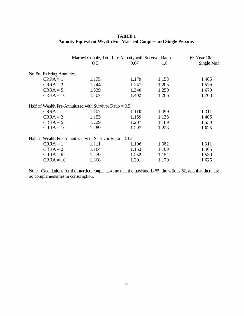
Table 1 presents our annuity equivalent wealth results for this “base case couple.” There are

two central findings. First, the value of annuitization is lower for the married couple than for a

"comparable" single individual. Second, the value of annuitization rises with risk aversion, and with the

age of the couple. These results parallel findings for single individuals.

Table 1 reports findings for various sets of parameter choices. The columns of the table show

alternative assumptions about φ, the ratio of survivor annuity income from the privately-purchased

annuity to the income received by the couple when both are alive. We consider the three most common

survivor benefit ratios of 1/2, 2/3, and 1. We also consider four different levels of risk aversion,

including a relative risk aversion coefficient of 1 (log utility), 2, 5, and 10.

The table also shows three different scenarios with regard to pre-existing annuity income. The

top panel corresponds to the case in which there is no pre-existing annuity. The middle panel assumes

the couple begins with half its wealth in a pre-existing real annuity that pays a survivor benefit equal to

one-half of the couple benefit. This is a stylized representation of the case in which both members of a

couple are entitled to equal Social Security benefits, and have half their wealth in Social Security. Upon

the death of the first spouse, the survivor will continue to receive only his or her own worker benefit. In

the bottom panel, we again assume that half of the couple's wealth is pre-annuitized, but now offer a

survivor payout equal to 67 percent of the couple’s benefit. This corresponds to a stylized case in

which the couple’s Social Security benefit consists of a primary worker benefit plus an additional 50

21

percent in dependent benefits. Upon the death of the first spouse, the Social Security benefit drops to

67 percent of the couple’s benefit.

The results in the first panel of Table 1 provide an illustration of our findings. When the

actuarially fair private annuity offers a joint life contract with a 50 percent survivor’s benefit to our base

case couple with log utility, access to annuitization is equivalent to a 17.5 percent increment to the

couple’s non-annuitized wealth. The annuity equivalent wealth, parameterized by α above, is 1.175.

Increasing risk aversion from 1 to 2 raises the annuity equivalent wealth from 1.175 to 1.244, and

further increases in risk aversion result in further increases in annuity equivalent wealth.

The results in the upper panel of Table 1 also suggest that the ratio of survivor benefits to

annuity payouts when both members of the couple are alive has a modest effect on annuity equivalent

wealth, at least at low levels of risk aversion. When the relative risk aversion coefficient is two, for

example, varying the survivor payout relative to the couple payout from 0.5 to 1.0 changes the annuity

equivalent wealth by only 0.044, i.e. 4.4 percent of initial non-annuitized wealth. All of the annuities that

we consider provide a constant nominal payout stream, so different survivor payout structures partly

affect the degree to which real benefits decline over time. Without consumption complementarities, the

survivor ratio of 0.67 provides the highest annuity valuation for most levels of risk aversion, though 0.5

is preferred for a risk aversion coefficient of 10. As can be seen, full survivor benefits are not optimal

for any of the levels of relative risk aversion that we consider. This is because upon the death of the first

spouse, the income required to provide the survivor with a given level of consumption declines.

Providing full survivor benefits gives too much income to the survivor at the expense of too low a

consumption level when both spouses are alive.

The final column of Table 1 provides a comparison to the case of a single male, age 65, who

maximizes an individual utility function and who does not have opportunities to pool risk within a

22

marriage. For all levels of risk aversion, the annuity equivalent wealth for couples is significantly lower

than that for single individuals. The difference between individual annuity valuation, and annuity valuation

by a married couple, is partly explained by the fact that risk sharing takes place within couples. If one

member of the couple lives an unexpectedly long life, there is some probability of inheriting resources

from an earlier-to-die spouse. This provides some mortality insurance, even without a formal annuity

contract.

The results in the two lower panels of Table 1 indicate how our findings change when the couple

has access to a pre-existing annuitized income stream such as Social Security or a defined benefit

pension plan. We assume that the pre-existing annuity benefit is indexed to inflation. Comparing the

results to the top panel, we see that the couple’s annuity equivalent wealth (now computed as a multiple

of initially non-annuitized wealth) declines when half of the couple's wealth is already annuitized. The

annuity equivalent wealth when the couple has some pre-existing annuity income is the ratio of the

couple’s non-annuitized wealth that would be required to make them as well off as if they were fully

annuitized. For all levels of risk aversion, and for all combinations of survivor benefits, the annuity

equivalent wealth is lower when the couple has some pre-annuitized wealth. This suggests that pre-

existing annuities reduce the demand for additional private annuities.

Table 2 explores the sensitivity of the results to alternative assumptions about the degree of

“jointness” in consumption. This table continues with our base case couple that consists of a 65-year

old man married to a 62-year old woman, but it now allows λ, the consumption complementarity

parameter, to vary. The first column again reports results for the case of no jointness (λ=0). The

second column assumes that half of all consumption is joint (λ=.5) and the third column assumes

complete jointness in consumption (λ=1). The jointness parameter λ does not affect the annuity

equivalent wealth in the case of log utility, so Table 2 reports results for risk aversion values of 2, 5, and

23

10. We restrict our attention to the case without pre-existing annuities, the case considered in the first

panel of Table 1, to focus on the effect of the private annuity survivor ratio. We vary the survivor ratio

on the privately purchased nominal annuity from 0.4 to 1.0 in increments of 0.1.

The jointness parameter clearly affects the desired survivor ratio. Without consumption

externalities, a survivor benefit ratio of 0.6 is preferred to the other ratios considered for all levels of risk

aversion that we consider. The preferred survivor ratio rises with the jointness parameter, with full

survivor benefits being preferred in the case of full consumption externalities (λ=1). Full jointness means

that a surviving widow, for example, needs just as much total income as she and her husband needed

when he was alive to sustain a given level of consumption. With full jointness in consumption, two can

consume for the price of one, so the death of a spouse does not reduce a household’s expenses.

Survivor benefits are more attractive when there are positive consumption externalities within a couple.

Table 3 explores the effect of the age of the husband and wife on the annuity equivalent wealth.

The table considers two levels of risk aversion, 1 and 5, but it confines attention to λ=0 and the case in

which the privately purchased annuity has a survivor benefit ratio of 0.67. We present results both for

the case of no pre-existing annuity wealth, and for the case in which half of wealth is pre-annuitized with

a survivor ratio of 0.5. The table shows that the annuity equivalent wealth increases with the age of

either spouse. Gaining access to annuities for two 70 year olds with log utility and no pre-existing

annuities is equivalent to a 24.2% increase in their wealth, compared to only 11.7% for two 55 year

olds. These age effects arise due to differences in mortality risk faced by the individuals. The rate of

return on an actuarially fair annuity consists of a mortality premium that is a function of the mortality

hazard. Older couples face higher mortality probabilities, and thus have more to gain from annuitization

than do younger couples.

24

4. Conclusions and Future Directions

This paper presents new results on the market for joint annuities and on the utility gains available

to married couples who are able to participate in actuarially fair annuity markets. A couple consisting of

a 65 year old man and a 62 year old woman find access to actuarially fair joint and survivor annuities

roughly equivalent to an 18% increase in non-annuitized wealth, assuming log utility. Their valuation of

annuities is even higher if risk aversion is higher or if the spouses are older at the date of annuitization.

We confirm previous findings for single individuals that suggest that pre-existing annuity wealth reduces

the demand for additional annuitization.

The results suggest that married couples value the opportunity to purchase joint and survivor

annuity products less than single individuals value the opportunity to purchase single life annuities.

Moreover, at high levels of risk aversion, annuity design features such as the relationship between the

annuity payouts for surviving spouses and the benefits paid to the couple when both members were alive

can have an important impact on the couple's valuation of the annuity.

Our estimates of the amount that couples would be prepared to pay to obtain joint and survivor

annuity products can be contrasted with the estimates of the expected present discounted value (EPDV)

of joint and survivor annuity payouts in Mitchell, Poterba, Warshawsky, and Brown (1999). Those

estimates suggested that for a 65 year old couple, the EPDV of the average annuity in the marketplace

is 84 percent of its initial premium. Because couples find annuities less valuable than single individuals,

couples may find that these “load factors” in the private marketplace are significant enough to deter

them from annuitizing their resources. Given the importance of married couples in the population age

groups that are most likely annuity buyers, this may help to explain the rather limited size of the annuity

market.

25

One of the important issues that we have not considered is the possible relationship between

mortality risk of married individuals. Frees, Carriere, and Valdez (1996) document a “broken heart

effect” in the mortality of married couples: conditional on the death of one spouse, the mortality risk of

the surviving spouse rises. Their calculations suggest that this effect reduces the expected discounted

value of joint and survivor annuity payouts by about five percent relative to what they would be without

this effect.

A second issue that we have not considered is the impact of bequest motives on the demand for

joint and survivor annuities. To the extent that couples value wealth that is left behind to their heirs, this

may lessen the value of annuitization. Jousten (1998) discusses in detail how one can model the utility of

gifts and bequests for the case of an individual life-cycle consumer. This analysis can be extended to the

couples’ context. We have not done this because there is remarkably little empirical guidance regarding

the parameterization of the utility of bequest function. One study that estimated the necessary utility

parameters for a bequest motive, Hurd (1987), estimated it for individuals and found the marginal utility

of bequests to be statistically indistinguishable from zero. Further work exploring the impact of bequests

in a couple’s context is left for future research.

A related issue that could explain the limited demand for private annuities is the potentially

important role of medical expense uncertainty. Both individuals and couples may be concerned about

the risk of future uninsured medical expenses (e.g., long-term care needs), and they may

correspondingly be reluctant to annuitize their resources. This explanation for limited annuity demand

has not yet been quantified, however, or evaluated using a well-calibrated model for health needs and

consumption demands.

A final issue for further study concerns the nature of the utility functions for men and women in

married couples. There is some evidence, for example from asset allocation patterns in defined benefit

26

plans, that women are more conservative investors than men are. If this reflects higher risk aversion,

then it may be appropriate to modify our assumption that men and women have the same preferences,

and hence sub-utility functions, in our analysis. More generally, it is possible that the couple's joint utility

function, which results from bargaining between the husband and the wife, is more complex than our

analysis suggests. Further progress in modeling the behavior of couples is likely to await clear empirical

evidence that bears on these issues.

27

REFERENCES

Auerbach, Alan, Laurence Kotlikoff, and David Weil (1992). "The Increasing Annuitization of theElderly: Estimates and Implications for Intergenerational Transfers, Inequality, and NationalSaving," NBER Working Paper 4182, Cambridge, MA.

Barsky, Robert B., F. Thomas Juster, Miles S. Kimball, and Matthew D. Shapiro (1997). “PreferenceParameters and Behavioral Heterogeneity: An Experimental Approach in the Health andRetirement Survey.” Quarterly Journal of Economics 107(May, 537-580.

Brown, Jeffrey (1999). “Private Pensions, Mortality Risk, and the Decision to Annuitize.” MITmimeograph.

Brown, Jeffrey R., Olivia S. Mitchell, and James M. Poterba. (1999). "The Role of Real Annuities andIndexed Bonds in an Individual Accounts Retirement Program." NBER Working Paper No.7005.

Frees, Edward W., Jacques Carriere, and Emiliano Valdez (1996), “Annuity Valuation with DependentMortality,” Journal of Risk and Insurance 63: 229-261.

Friedman, Benjamin, and Mark Warshawsky (1988). “Annuity Prices and Saving Behavior in theUnited States.” In Z. Bodie, J. Shoven, and D. Wise, eds., Pensions in the U.S. Economy(Chicago: University of Chicago Press), 53-77.

Friedman, Benjamin, and Mark Warshawsky (1990). ”The Cost of Annuities: Implications for SavingBehavior and Bequests.” Quarterly Journal of Economics 105: 135-154.

Holden, Karen (1997). “Women as Widows under a Reformed Social Security System,” in Prospectsfor Social Security Reform (Philadelphia: Pension Research Council, The Wharton School,University of Pennsylvania).

Hubbard, R. Glenn (1987). “Uncertain Lifetimes, Pensions, and Individual Saving.” In Z. Bodie, J.Shoven, and D. Wise, eds., Issues in Pension Economics. Chicago: University of ChicagoPress, 175-206.

Hurd, Michael (1987). “Savings of the Elderly and Desired Bequests,” American Economic Review77: 298-312.

Hurd, Michael (1989). “Mortality Risk and Bequests,” Econometrica 57: 779-813.

Hurd, Michael (1999). “Mortality Risk and Consumption by Couples,” NBER Working Paper 7048. Cambridge, MA.

Jousten, Alain (1998). The Economics of Gifts and Bequests. Ph.D. dissertation, MIT EconomicsDepartment, Cambridge MA.

28

Juster, F. Thomas and John Laitner (1990). "The TIAA-CREF Data Base: A Special Purpose Data Setfor the Analysis of Life-Cycle Saving Behavior," working paper, Institute for Social Research atthe University of Michigan.

King, Francis (1996). "Trends in the Selection of TIAA-CREF Life-Annuity Income Options, 1978-1994," TIAA-CREF Research Dialogues, Issue 48.

Kotlikoff, Laurence J. and Avia Spivak (1981). “The Family as an Incomplete Annuities Market”.Journal of Political Economy 89: 372-391.

Laibson, David, Andrea Repetto, and Jeremy Tobacman (1998). “Self Control and Saving forRetirement.” Brookings Papers on Economic Activity. 1.

Laitner, John (1997). “Intergenerational and Interhousehold Economic Links.” In Mark Rosenzweigand Oded Stark, eds., Handbook of Population and Family Economics: Volume 1A. (Amsterdam: North Holland).

Laitner, John and F. Thomas Juster (1996). "New Evidence on Altruism: A Study of TIAA-CREFRetirees," American Economic Review 86: 893-908.

LIMRA International (1996). “The 1995 Individual Annuity Market - Sales and Assets”. AnnuityResearch. Hartford: LIMRA International.

LIMRA International (1997). “Product Design Series: Immediate Annuities.” Annuity Research. Hartford: LIMRA International.

Mehra, Rajnish and Edward Prescott (1985). “The Equity Premium: A Puzzle.” Journal of MonetaryEconomics 15, 145-161.

Mitchell, Olivia, James Poterba, Mark Warshawsky, and Jeffrey Brown (1999). "New Evidence onthe Money's Worth of Individual Annuities," American Economic Review (forthcoming).

Yaari, Menahem E. (1965). “Uncertain Lifetime, Life Insurance, and the Theory of the Consumer,” Review of Economic Studies 32: 137-150.

Yagi, Tadashi, and Yasuyuki Nishigaki, 1993, “The Inefficiency of Private Constant Annuities,” Journalof Risk and Insurance 60(3): 385-412.

</ref_section>

29

TABLE 1Annuity Equivalent Wealth For Married Couples and Single Persons

Married Couple, Joint Life Annuity with Survivor Ratio 65 Year Old

0.5 0.67 1.0 Single Man

No Pre-Existing AnnuitiesCRRA = 1 1.175 1.179 1.158 1.465CRRA = 2 1.244 1.247 1.205 1.576CRRA = 5 1.339 1.340 1.250 1.679CRRA = 10 1.407 1.402 1.266 1.703

Half of Wealth Pre-Annuitized with Survivor Ratio = 0.5CRRA = 1 1.107 1.110 1.099 1.311CRRA = 2 1.153 1.159 1.138 1.405CRRA = 5 1.229 1.237 1.189 1.530CRRA = 10 1.289 1.297 1.223 1.625

Half of Wealth Pre-Annuitized with Survivor Ratio = 0.67CRRA = 1 1.111 1.106 1.082 1.311CRRA = 2 1.164 1.153 1.109 1.405CRRA = 5 1.279 1.252 1.154 1.530CRRA = 10 1.368 1.301 1.170 1.625

Note: Calculations for the married couple assume that the husband is 65, the wife is 62, and that there areno complementaries in consumption.

30

TABLE 2Effect of Consumption Complementary, Measured by λ, on Annuity Equivalent Wealth

CRRA = 2 λ=0 λ=.5 λ=1Survivor Ratio =

.4 1.201 1.153 1.120

.5 1.230 1.190 1.165

.6 1.244 1.213 1.194

.7 1.248 1.225 1.213

.8 1.236 1.231 1.228

.9 1.222 1.226 1.2291.0 1.205 1.217 1.230

CRRA = 5 λ=0 λ=.5 λ=1Survivor Ratio =

.4 1.312 1.152 1.057

.5 1.339 1.216 1.142

.6 1.345 1.256 1.197

.7 1.335 1.274 1.233

.8 1.313 1.280 1.256

.9 1.284 1.277 1.2681.0 1.250 1.264 1.272

CRRA = 10 λ=0 λ=.5 λ=1Survivor Ratio =

.4 1.388 1.035 < 1

.5 1.407 1.175 1.021

.6 1.412 1.255 1.131

.7 1.394 1.293 1.204

.8 1.354 1.298 1.249

.9 1.308 1.293 1.2721.0 1.266 1.280 1.278

Notes: All calculations assume that the couple does not have any pre-existing annuity wealth. Theparameter λ indicates the degree of consumption complementarity; see text for further discussion. Calculations are for a married couple in which the husband is 65, and the wife is 62.

31

TABLE 3Effect of Age Differentials on a Couple’s Annuity Equivalent Wealth

Age of Husband

Age of Wife 55 60 65 70

CRRA = 1, Privately Purchased Annuity with Survivor Ratio = 0.67, No Pre-Existing Annuities

55 1.117 1.131 1.146 1.160 60 1.133 1.151 1.170 1.188 65 1.150 1.171 1.194 1.215 70 1.168 1.193 1.217 1.242

CRRA=1, Privately Purchased Annuity with Survivor Ratio 0.67, Half of Wealth Pre-Annuitized withSurvivor Ratio 0.5

55 1.070 1.082 1.094 1.103 60 1.082 1.095 1.105 1.118 65 1.094 1.104 1.118 1.132 70 1.103 1.117 1.131 1.146

CRRA = 5, Privately Purchased Annuity with Survivor Ratio = 0.67, No Pre-Existing Annuities

55 1.216 1.243 1.261 1.283 60 1.253 1.281 1.320 1.339 65 1.286 1.334 1.366 1.411 70 1.322 1.374 1.433 1.475

CRRA=5, Privately Purchased Annuity with Survivor Ratio 0.67, Half of Wealth Pre-Annuitized withSurvivor Ratio 0.5

55 1.161 1.178 1.184 1.193 60 1.181 1.193 1.216 1.252 65 1.193 1.221 1.265 1.291 70 1.215 1.265 1.294 1.326

Notes: All calculations assume that there are no consumption complementarities between the husband andthe wife.

32

Figure 1: Individual and Joint Survival

0

0.2

0.4

0.6

0.8

1

1 5 9

13

17

21

25

29

33

37

41

45

49

53

Pro

b(S

urv

ival

)

Male 65

Female 65

Joint 65/65