John Methven, Department of Meteorology - ECMWF · John Methven, Department of Meteorology. ......

© University of Reading 2007 www.reading.ac.uk

ECMWF Annual Seminar

Diagnostics of the Extratropics

John Methven, Department of Meteorology

Diagnostics vs prognostics

Diagnosis: determine properties of current state (of atmosphere) given observations now and in recent past. Involve eqns relating variables at one instant in time.

Prognosis: forecast properties based on a diagnosis of the current state. Integrating eqns with time derivatives.

There are endless ways of diagnosing the atmosphere (e.g., correlating temperature in Reading with surface pressure in Iceland).

But, the most useful diagnostics are those which relate to conceptual and theoretical models of the way in which atmosphere evolves.

Even if a complex numerical model is required to produce an accurate forecast, powerful diagnostics enable us to anticipate what will happen next and to understand model failings.

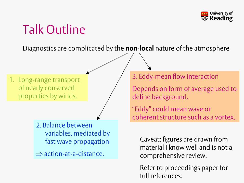
Talk Outline

Diagnostics are complicated by the non-local nature of the atmosphere

1. Long-range transport of nearly conserved properties by winds.

2. Balance between variables, mediated by fast wave propagation

action-at-a-distance.

3. Eddy-mean flow interaction

Depends on form of average used to define background.

“Eddy” could mean wave or coherent structure such as a vortex.

Caveat: figures are drawn from material I know well and is not a comprehensive review.

Refer to proceedings paper for full references.

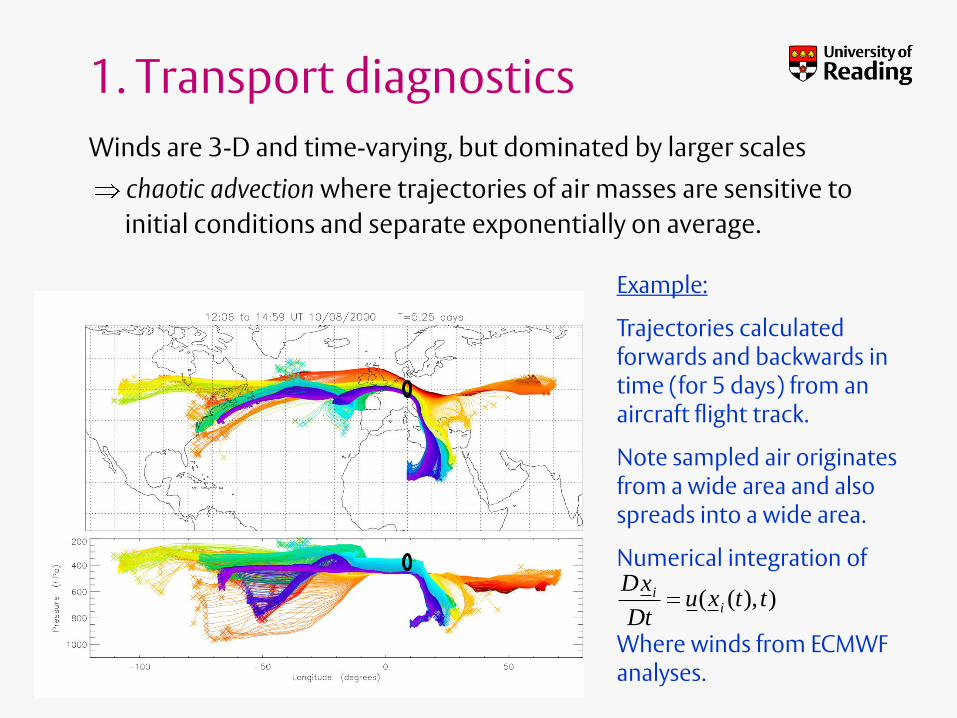
1. Transport diagnostics

Winds are 3-D and time-varying, but dominated by larger scales

chaotic advection where trajectories of air masses are sensitive to

initial conditions and separate exponentially on average.

Example:

Trajectories calculated forwards and backwards in time (for 5 days) from an aircraft flight track.

Note sampled air originates from a wide area and also spreads into a wide area.

Numerical integration of

Where winds from ECMWF analyses.

( ( ), )ii

Dxu x t t

Dt

Are trajectories predictable?

Can observe chemical and thermodynamic tracers with aircraft to establish air-mass identities.

BUT need to forecast air-mass trajectories in order to direct aircraft to intercept the same air several times over a long range.

Motivation for the ITCT-Lagrangian 2K4 Experiment which took place within the framework of the ICARTT campaign in summer 2004:

Sample polluted air masses leaving the continental BL.

Follow across Atlantic since no emissions after USA.

Deduce chemical transformation en route.

Scale of problem requires several coordinated research aircraft.

JGR, ICARTT special issue

Fehsenfeld et al [2006] – campaign overview

Methven et al [2006] – Lagrangian experiment

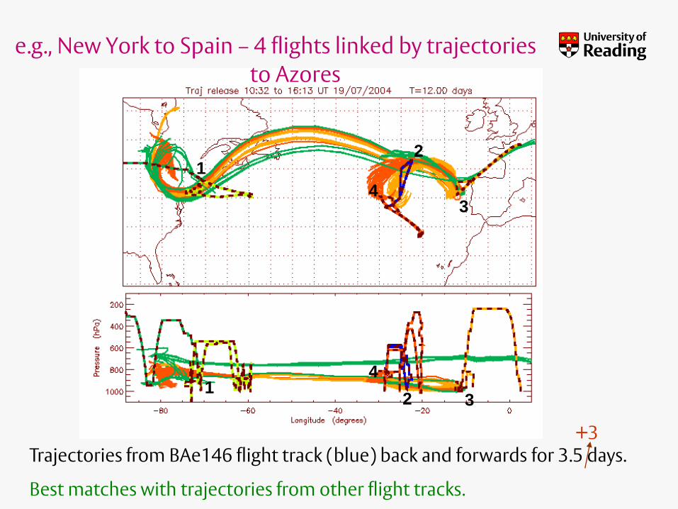
e.g., New York to Spain – 4 flights linked by trajectories

12

3

Trajectories from BAe146 flight track (blue) back and forwards for 3.5 days.

Best matches with trajectories from other flight tracks.

2 31

4

4

+3

to Azores

Did the aircraft sample the sameair mass many times?

Two independent matching methods:

1. Trajectory models driven by met. analyses2. Hydrocarbon fingerprints (bottled air samples)

Search for coincident matches:two samples with matching HC fingerprint are also linked by matching trajectories.

Quality of matches assessed using independent observations of thermodynamic tracers

Lagrangian match quality evaluated with temperature and humidity observations

Coincident HC/FLEXPART matches

Hydrocarbon matches

Pairing random time points

Trajectory matches

Coincident matches strongly peaked (almost adiabatic)

New York -Ireland.Mixing and cooling in North Atlantic MBL.

Latent heat release (ascent).

Trajectory-only matches good in theta. Analysis close to obs.

Coincident HC/traj matches

Matching HCs alone does not make a Lagrangian match

D /Dt D e/Dt

NY-Spain-Azores photochemistry simulationO

zon

e →

Nit

ric

acid

→C

O →

NO

→

Time →

USA day 0

Azores day 4

Spainday 7

Azores day 10

Long-lived

Short-lived

(absent at night)

Less reactive but sensitive to deposition

Why are trajectory calculations so accurate?

trajectories

Chaotic advection tracer “cascades” to small scales.

Occurs even though winds are dominated by large scales.

Can we use low resolution winds?

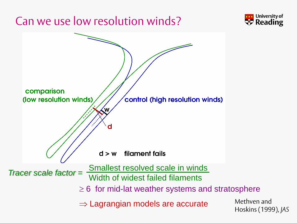
Can we use low resolution winds?

Tracer scale factor =Smallest resolved scale in winds

Width of widest failed filaments

6 for mid-lat weather systems and stratosphere

Lagrangian models are accurate Methven and Hoskins (1999), JAS

Reverse domain filling trajectories

Finescale tracer structure can be diagnosed by calculating many back trajs from a dense 3-D grid and colouring each grid-point by value of tracer at origin.

e.g., Sutton et al [1994], JAS

Back trajectories from points A, S and E on section XY

Sampled using MRF aircraft in 2000. Methven et al [2003], JGR

Meteosat WV chan dry intrusion

X Y

S

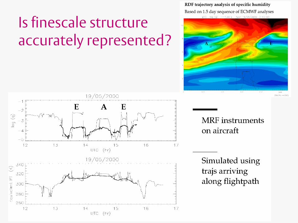
Is finescale structure accurately represented?

Allowing for non-conservation

• RDF trajectory reconstructions assume tracer conservation.

• Strong gradients arise as air masses of different origins are brought together by strain flow (tracers are long-lived relative to Lagrangian decorrelation timescale ~1 day in mid-lats).

• As trajectory length in time increases, RDF structure becomes increasingly finescale until unrealistic.

• Relevant trajectory length is determined by non-conservative processes following air-masses.

Next level of sophistication is to use simple models along trajs.

Application for water vapour. (e.g., Sherwood [1996], J.Clim.; Pierrehumbert and Roca [1998], GRL)

Advection-condensation model (1)

qmin = min[ qsat ] (occurs at t=-τ min)

qtraj = min[ q(-T), qmin ]

Back trajectories from

coordinates of radiosonde.

T, q interpolated from analyses to

trajectory coords.

RHtraj.

RHanalysis

100hPa

RHtraj

RHanalysis

100hPa

black areas

grey areas

Cau, Methven and Hoskins (2005), JGR, 110, d06110

Sonde observations of RH in TOGA COARE expt

Dry events simulated using trajectories

Advection-condensation model (2)

qtraj = qsat at last condensation, t=-τ last

qtraj = q(-T) if saturation does not occur

Model allowing for re-

moistening implicit in

analyses

Cau, Methven and Hoskins (2007), J.Climate

Time since last condensation

Time since min(qsat)

along any traj

Time since last

condensation event for

dry air masses

min(qsat) equally likely to occur at any time along a traj.

Last condensation most likely 2-3 days before dry event.

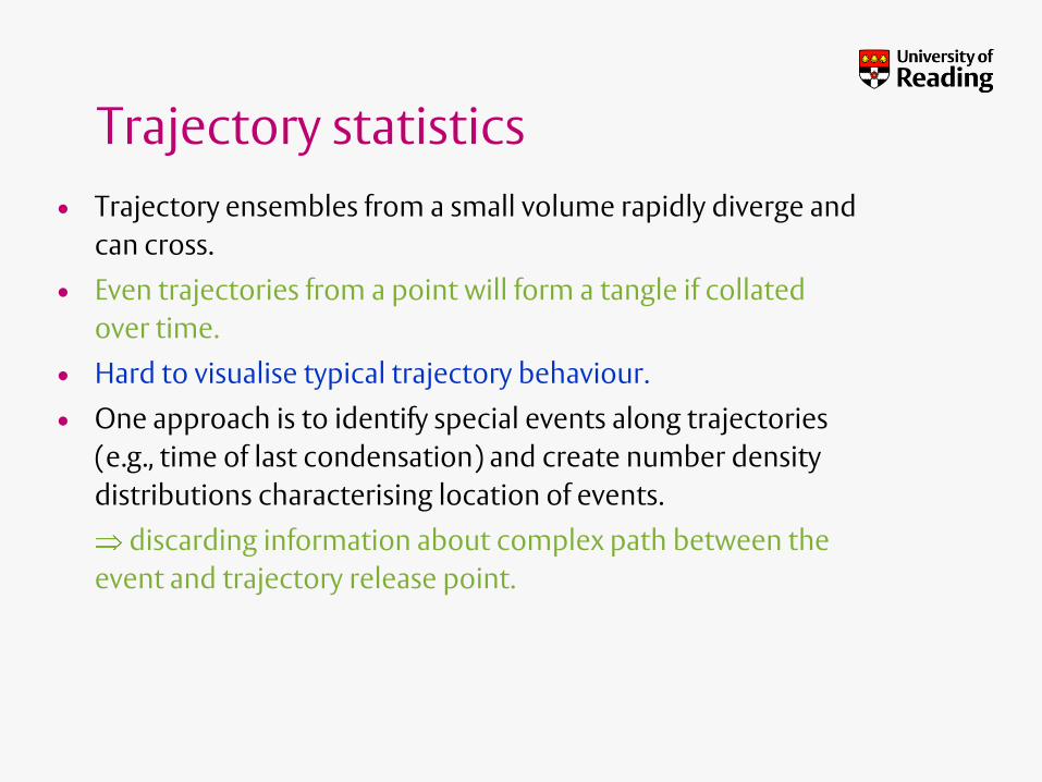
Trajectory statistics

• Trajectory ensembles from a small volume rapidly diverge and

can cross.

• Even trajectories from a point will form a tangle if collated

over time.

• Hard to visualise typical trajectory behaviour.

• One approach is to identify special events along trajectories

(e.g., time of last condensation) and create number density

distributions characterising location of events.

discarding information about complex path between the

event and trajectory release point.

Preferred regions for condensation

Dry regions in subtropics

Number density of dry events

(RH<20%) at all levels during

Jan 1993.

Integrates to one over sphere.

Zero outside 40S-40N band.

Number density of last

condensation events.

“Density of origin” for dry air

arriving in 40S-40N band.

Far from uniformly distributed

and often in extratropics.

Origins for isolated dry regions

Dry regions are isolated by boxes.

Contours show corresponding density of origin.

Many contributors to each dry region.

Destination of air saturating in isolated regions

Condensation events within isolated boxes.

Contours show arrival locations of these dry air masses.

Each condensation region contributes to one/two dry regions.

Transport processes linking dry air to its origins

Descending air

behind cyclones.

Transient events in

storm tracks.

Air descending

into lower trop

around A/C

Nearly steady jet minimum.

Descent crossing equatorward flank

of jet exit from UT.

Ascent into jet entrance in UT, then

radiative descent in jet.

Stagnation in UT over

tropical Atlantic

1. Conclusions on Transport

Trajectory calculations are surprisingly accurate.

Verification with observations is difficult, but possible using tracers.

Trajectories are sufficiently predictable to conduct Lagrangian aircraft experiment.

Finescale tracer structure can be reproduced using reverse domain filling trajectory calculations for 3D domains – used forecast mode during aircraft campaigns.

Simple advection-condensation models enable diagnosis of the water vapour distribution and the “origin” of unsaturated air.

Number density distributions are useful reduction of Lagrangian information.

e.g., Fueglistaler et al (2005), JGR characterise entry of dry air into stratosphere.

If small Rossby number, Ro=V/(fL), the last two terms dominate

Geostrophic flow e.g., zonally symmetric flow

Define geostrophic streamfunctionGeostrophic flow components are then

2. Balance in the Extratropics

Geostrophic balance

Horizontal components of momentum equation

(use planar approx. Valid if L/a«1 where a=Earth’s radius)

0

'g

r

p

f

1Dv pfu

Dt yy-component

1g

pu

f y

g

guy

g

gvx

Hydrostatic balance

Consider vertical momentum equation:

2

0

1 'g gu b

z z y f y

1Dw pg

Dt z

0

' '

r

Dw g p

Dt z

0

0

''

ggb f

z

Anelastic approximation. ’/ « 1 and H H

Buoyancy

Hydrostatic approximation. H/L « 1

2

0

1 'g gv b

z z x f x

Together with geostrophic balance we obtainthermal wind balance which is fundamental in atmosphere and ocean.

Predicting geostrophic flow evolution

Geostrophic and hydrostatic balance are diagnostic

- the time derivatives have been neglected.

Flow evolution depends on ageostrophic flow: ag g

ag g

ag

u u u

v v v

w w

0 0( ) 0ag

Dvf f u f u

Dt

Quasi-geostrophic theory is obtained at next order and predicts vorticity evolution:

and evolution of buoyancy:

0 0

( )1( ) r

g g

r

wD f y f

z

2' 0gD b N w

Vortex stretching increases absolute

vorticity following geostrophic flow

Advection of reference buoyancy

downwards increases buoyancy

following geostrophic flow

g g gD u vt x y

Define geostrophic

material derivative

e.g.,

QG potential vorticity

Vorticity and buoyancy evolution both depend on vertical motion, w.

Eliminating w from the two equations gives:

0gD q

Meaning that QG potential vorticity, q, is conserved following the geostrophic flow, where

2 2 2

00 2 2 2

1g g g

r

r

fq f y

x y z N z

Given distribution of q and boundary conditions, can invert PV

' ( )gq q f L to find1( ')g L q

Solution of QG system is to advect QGPV contours with the geostrophic flow (like a tracer) over one time-step. Then invert the new PV distribution to infer new flow and buoyancy:

g

guy

g

gvx

0'g

b fz

Action-at-a-distanceAssuming density and N are constants and re-scaling the height

coordinate so that 0( / )z N f z

2 2 22

22 2' g gq

x y z

Poisson equation. Other examples from physics:

q’=point charge; =electric field potential

q’=force at a point on drum; =drum skin displacement

Means that a point PV anomaly induces flow far away.

The induced streamfunction is symmetrical about point in re-scaled coordinates.

natural aspect ratio 0

100L N

H f

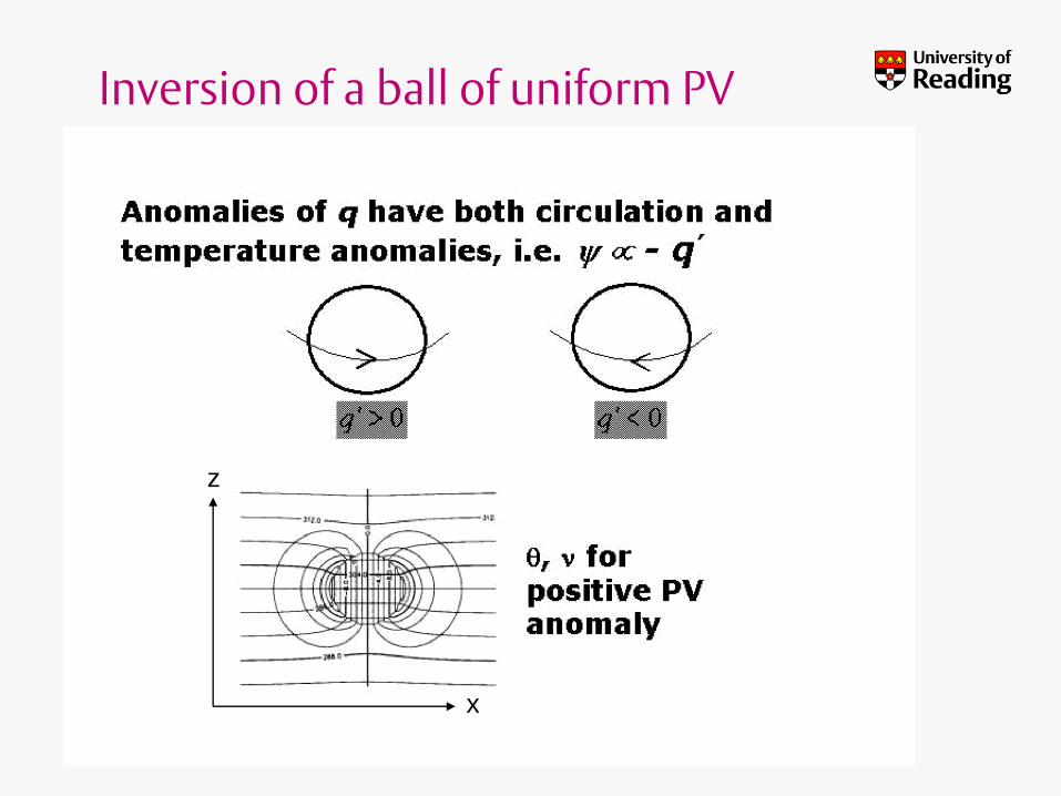
Inversion of a ball of uniform PV

x

z

Rossby waves

Rossby waves propagate on horizontal PV gradients.

low PV

high PV

0y

q

Air displaced to south carries high PV and forms +ve q’

q’>0 induces cyclonic circulation

advects air southwards on western flank

wave pattern propagates westwards

2

1p

qc u

k yPhase speed: Fig: Hoskins, McIntyre and Robertson

(1985), QJ

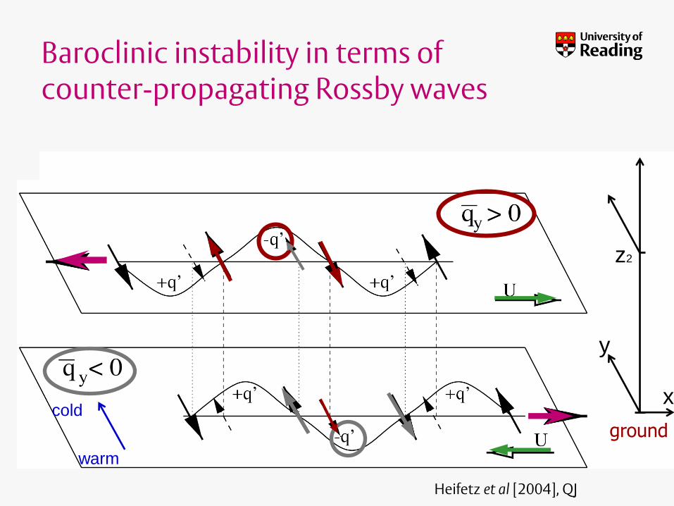
Baroclinic instability in terms of counter-propagating Rossby waves

ground

z2

y

x

warm

cold

Heifetz et al [2004], QJ

PV diagnostics

Ertel PV is conserved by the unapproximated dynamical equations

following adiabatic, frictionless flow.

• Pragmatic approach is to calculate Ertel PV as diagnostic from model

variables

approximately follows motion of air along surfaces of constant

potential temperature (isentropic surfaces)

imagine the flow and stratification anomalies associated with PV

anomalies and they way in which they would influence evolution

• More quantitatively make a balance approximation and invert the

PV distribution or portions of it.

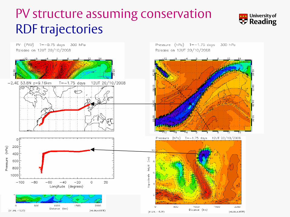
PV structure assuming conservationRDF trajectories

Air mass: history of ascent

Change in pressure along trajectory before arrival over UKGreen/blue=ascent

1.75 days travel

0.75 days travel

w = warm conveyor belt of cyclone over UK

w

w

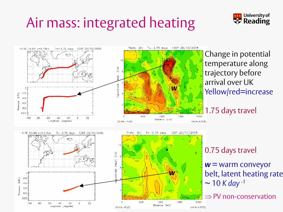
Air mass: integrated heating

w

w

0.75 days travel

w = warm conveyor belt, latent heating rate ~ 10 K day -1

PV non-conservation

Change in potential temperature along trajectory before arrival over UKYellow/red=increase

1.75 days travel

Sensitivity of model PV to representation of diabatic processes

Experiments running the global and 12km LAM versions of the Met Office Unified Model

(Jeffrey Chagnon, NCAS-weather)

Same case as RDF example. Shown 4 days prior to forecast bust over Europe identified by Thomas Jung.

Same cross-section taken.

Global vs mesoscale model PV

Tracking non-conservative changes in PV

• New set of diagnostics has been developed by Bob Plant (Reading)

based on a Lagrangian decomposition of the PV field.

• Full PV conservation equation can be written:

p

p

DqS

Dtwhere Sp denotes the Lagrangian tendency resulting from one physical process in model

• Tracers qp are initialised as zero but experience only one of the Sp

terms as well as being advected by the semi-Lagrangian scheme.

each tracer shows accumulated contribution of one process to PV.

passive p

p

q q q

Global vs mesoscale model PV

Accumulated PV tracers for the effects of convection and large-scale rain parameterisations in LAM model.

PV error on 315 K(forecast - analysis)

III:EnsemblesTypical forecast errors in upper-level PV field

[pvu]

from Marco Didone and Huw Davies, ETH, Zurich

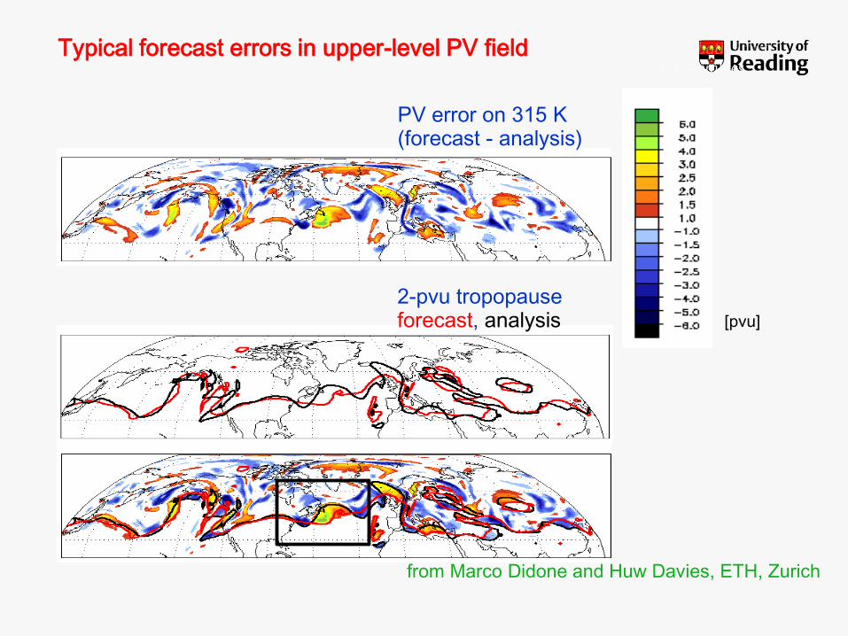
from Marco Didone and Huw Davies, ETH, Zurich

PV error on 315 K(forecast - analysis)

III:EnsemblesTypical forecast errors in upper-level PV field

[pvu]

2-pvu tropopauseforecast, analysis

analysis forecastpvu

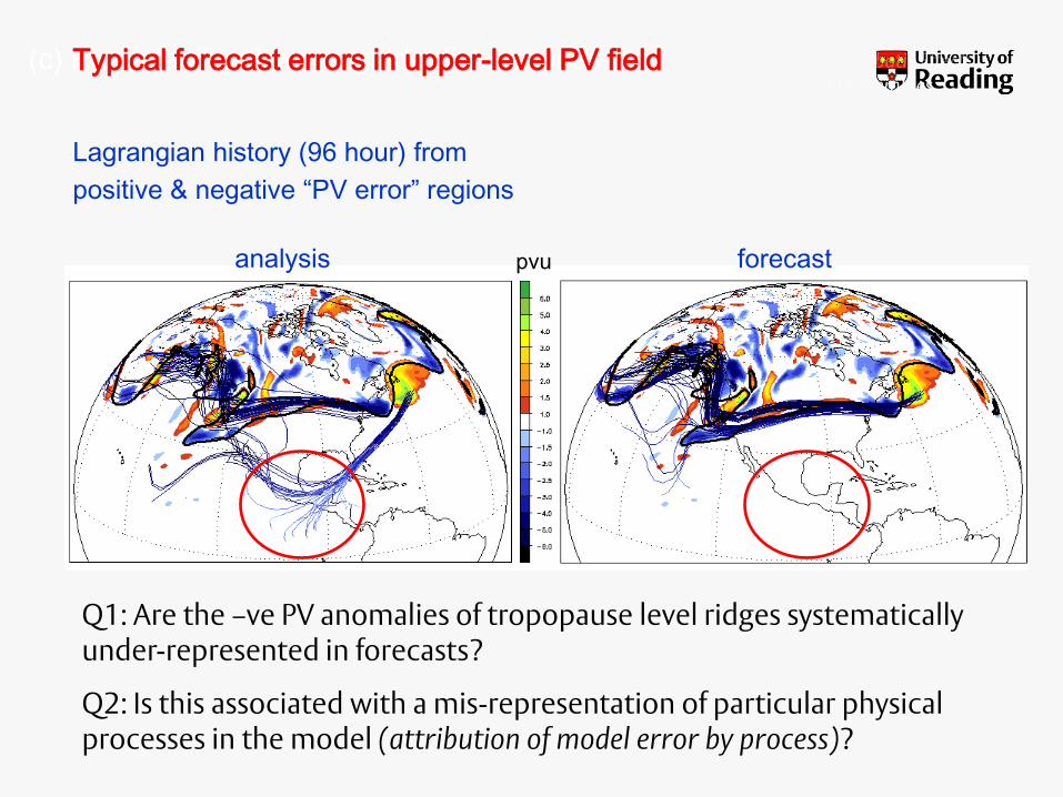
(c) Predictability & wave-guide disturbancesIII:Ensembles

Typical forecast errors in upper-level PV field

Lagrangian history (96 hour) from

positive & negative “PV error” regions

Q1: Are the –ve PV anomalies of tropopause level ridges systematically under-represented in forecasts?

Q2: Is this associated with a mis-representation of particular physical processes in the model (attribution of model error by process)?

T-NAWDEX

THORPEX- North Atlantic Waveguide and Downstream Impact Experiment

Has been proposed by the THORPEX working group Predictability and

Dynamical Processes for the European THORPEX Science Plan.

Its overarching scientific goal is to investigate in detail the

physical processes that are primarily responsible for degradation in 1-7

day forecast skill in global prediction systems and of their representation in

NWP models.

An international field experiment is proposed for autumn 2012 observing

diabatic processes within Atlantic weather systems.

Piecewise PV inversion (PPVI)

• The PV diagnostics discussed so far relate only to the material

conservation property of PV.

• If one believes that a localised PV anomaly has been mis-

represented, it would be desirable to find the consequent impact.

• PPVI involves isolating a PV anomaly and inverting it to obtain

associated flow and temperature anomalies (assuming an

appropriate form of balance).

• These diagnostically related anomalies are then subtracted from the

full fields, and the modified state is integrated to find new forecast.

Davis and Emanuel (1991), MWR

Hakim, Keyser and Bosart (1996), MWR

-6 days

A

B

C

D

Rossby wave

PV

reservoir

E blocking

PVU

PPVI example: composite of events leading

to a cut-off low in Eastern Atlantic

Peter Knippertz (Leeds), Luise Frohlich and Florian Maier (Mainz)

latitu

de

system-relative longitude

–180 –150 –120 –90 –60 –30 0 +30 +60 +90 +120 +150 +180

-4 days

AB

C

DE

Intensification of

Rossby wave

PVU

COMPOSITE STUDY

System-relative composite of PV anomalies in 400–100 hPa

North Atlantic, winter half year (Oct.–Mar.), 87 systems

latitu

de


–180 –150 –120 –90 –60 –30 0 +30 +60 +90 +120 +150 +180

-3 days

A

B

C

D

FE

Development of

negative PV anomaly F

deformation of

PV reservoir

PVU

COMPOSITE STUDY



latitu

de


–180 –150 –120 –90 –60 –30 0 +30 +60 +90 +120 +150 +180

-2 days

A

BC F

E

D

D*

Development of

PV streamer

PVU

COMPOSITE STUDY



latitu

de


–180 –150 –120 –90 –60 –30 0 +30 +60 +90 +120 +150 +180

-1 days

A

BC

FE

D

D*

merging of C & D

cut-off of D*

PVU

COMPOSITE STUDY



latitu

de


–180 –150 –120 –90 –60 –30 0 +30 +60 +90 +120 +150 +180

+0 days

AB

C

D

FE

D*Rossby-

wave breaking

PVU

COMPOSITE STUDY



latitu

de


–180 –150 –120 –90 –60 –30 0 +30 +60 +90 +120 +150 +180

PV at 320 K

1200 UTC

05 January 2002

(+36h)

Control simulation

6.0

5.0

4.0

3.0

2.0

1.5

1.0

0.5

0

PVU

CF E

D

D*

B

B C

D

F E

D*

Global model

(GME) of the

German Weather

Service (DWD)

PPVI SENSITIVITY EXPERIMENTS

PV at 320 K at 0000 UTC 04 January 2002 (+00h)

6.0

5.0

4.0

3.0

2.0

1.5

1.0

0.5

0

Control simulation

PVU

Modified

initial conditions C

C F

ED

D* C F

ED

D*

PV inversion



6.0

5.0

4.0

3.0

2.0

1.5

1.0

0.5

0

PVU

CF E

D

D*

C FE

D

D*

B B

Control simulationModified

initial conditions C



6.0

5.0

4.0

3.0

2.0

1.5

1.0

0.5

0

PVU

Modified

initial conditions E

ED

E

D

Control simulation



6.0

5.0

4.0

3.0

2.0

1.5

1.0

0.5

0

PVU

Modified

initial conditions E

CF E

D

D*C F

ED

D*BB

Control simulation



6.0

5.0

4.0

3.0

2.0

1.5

1.0

0.5

0

PVU

C F

ED

D*

No latent heating

C F

ED

D*

Control simulation

PROCESS SENSITIVITY EXPERIMENT


6.0

5.0

4.0

3.0

2.0

1.5

1.0

0.5

0

PVU

CF

E

D

D*

BCF E

D

D*

B

Control simulation No latent heating

PROCESS SENSITIVITY EXPERIMENT

Most important prerequisite for

formation of D* is dipole D & E.

Rossby wave (B&C) & latent

heating are of secondary

importance.

Further tests and different case

studies will show how robust

this result is.

Existence of stable precursors

up to 6 days ahead suggests

some degree of predictability.

BC

D

FE

D*

latent

heating

SUMMARY OF PPVI STUDY

2. Balanced flow diagnostics

• Diagnose PV from primitive equation model, rather than integrate an explicitly balanced model.

• PV evolution is dominated by advection along isentropic surfaces.

• Finescale PV structure can be reconstructed using RDF trajectories.

• Integrated effects of non-conservative processes in a model can be diagnosed using PV tracers reveals differences between models.

• Piecewise PV inversion can be a useful tool

– However, sense behind spatially isolating a PV anomaly is debatable when part of a wave rather than cut-off vortex.

• Egger (2008), JAS; Methven and de Vries (2008), JAS

– Revising forecasts by PV modification on the basis of water vapour channel satellite imagery gives mixed results in forecast skill.

• Demirtas and Thorpe (1999), MWR; Swarbrick (2001), Met. Apps.

3. Mean flow and eddies

Theories describing the evolution of disturbances, including waves and

vortices, include a “basic state” upon which the disturbance evolves.

However, the atmosphere is complex with large-amplitude time-

varying disturbances. The “background state” must be identified

with some form of average. Candidates are:

1. Time average (at fixed points)

Cannot evolve!

The averaged state is not a solution on its own, and “interactions” with

waves contrive to make it steady.

e.g., local emissions could dominate the averaged state.

2. Zonal average (Eulerian)

Adiabatic eddy fluxes

Zonal average fluctuates as rapidly as the waves.

(Eulerian) Zonal Average

z

Space and Time Filtering

Can the background be extracted by a spatial or temporal filter?

BUT, no spectral gap. More similar to a power law scale invariance.

Wave-background partition depends on filter “scale interaction” is artificial.

By itself the filtered state is not a solution to the primitive equations.

Nastrom and Gage

(1985), JAS, 42, 950.

Scaling of wind and

temperature covariance

from regular aircraft

measurements (GASP).

k

An alternative in tracer relative coordinates

Example of a 2D tracer field Its background state

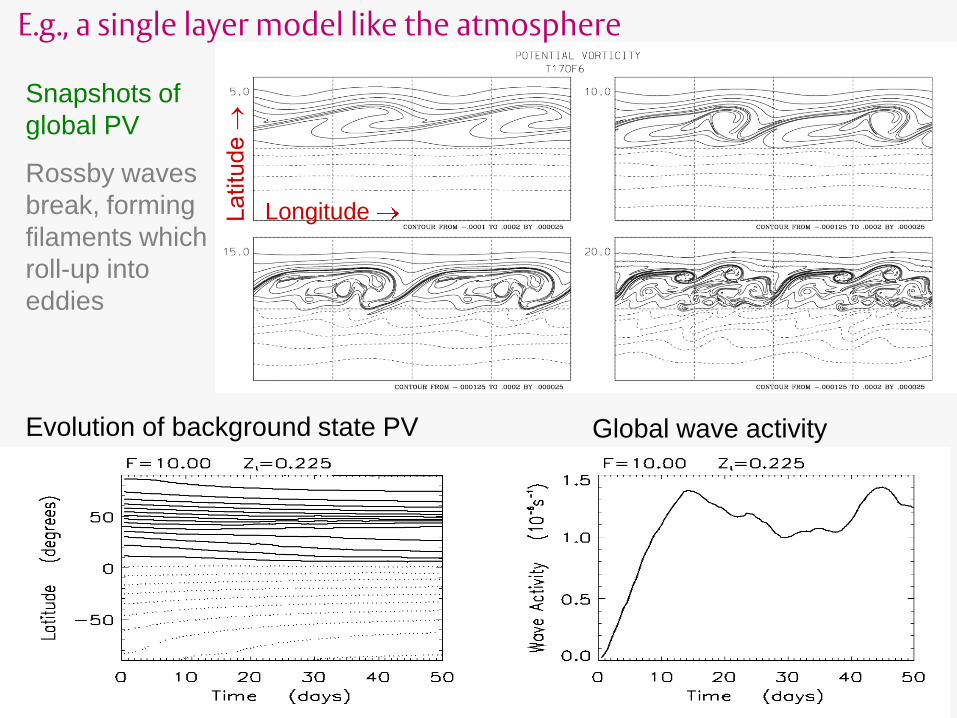
Evolution of background state PV Global wave activity

Snapshots of

global PV

Rossby waves

break, forming

filaments which

roll-up into

eddies

Longitude

E.g., a single layer model like the atmosphere

Modified Lagrangian Mean

• Background state PV is zonally symmetric.

• Obtained by adiabatic rearrangement from wavy 2D state, such that the

area enclosed by each PV contour is conserved.

• Equivalent latitude = latitude at the southern edge of a polar cap with

area matching the area enclosed by wavy PV contour.

– Used by stratospheric community to diagnose ozone, water etc in polar

vortex relative frame (McIntyre, 1980; Norton, 1994; Lary et al, 1995).

• A 2D MLM state can be found by re-arrangement of 3D wavy state

conserving mass and circulation enclosed by PV contours.

• Can only evolve through non-conservative processes, so slowly varying.

' '' 0

q q qu v

t x y

21 '' ' 0

2y

qv q

t qx q’ and take zonal average

. 0A

Ft

Taylor identity

Conservation law

Wave activity conservation

Theory of wave-mean flow interaction hinges on wave activity

conservation laws. Linear QG version obtained from PV eqn:

A = wave activity density F = Eliassen-Palm flux

0

2

' '' ',

f v bF u v

N

Similar conservation law is obtained for large-amplitude disturbances in the primitive equations, but only if background defined by the MLM state (Haynes, 1988, JAS).

Rossby wave packets

Flux of wave activity in latitude-height section is associated with group

velocity of Rossby wave packets, by formula:

gF c A

Wave activity increases where wave packets converge.

Ray tracing technique calculates paths of packets from group velocity.

Packet transports wave momentum great distances.

Considering the vorticity equation on a pressure level, Rossby waves are forced by the Rossby wave source, S:

Hayes [1977], Proc. Roy. Soc. London Edmon, Hoskins and McIntyre [1980], JAS

. .( )v v St

Sardeshmukh and Hoskins (1988), JAS

Teleconnection patterns

Some rays are followed frequently because Rossby wave forcing

occurs in same place and ray determined by flow.

forcing

2

1 3

213

Stationary Rossby wave response to forcing in W. Pacific [Ambrizzi and Hoskins, 1993]

Correlation of height of 500hPa surface with time series at P.

Wallace and Gutzler [1981] called it the Pacific North American pattern.

An example of a teleconnection pattern

Linking extreme seasons to teleconnection

patterns: e.g.,UK, Autumn 2000

Mike Blackburn, NCAS-climate

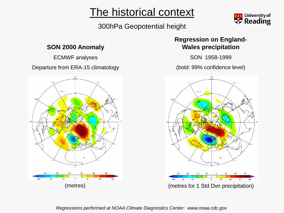
The historical context

Regressions performed at NOAA Climate Diagnostics Center: www.noaa.cdc.gov

Regression on England-

Wales precipitation

SON 1958-1999

(bold: 99% confidence level)

(metres for 1 Std Dvn precipitation)

SON 2000 Anomaly

ECMWF analyses

Departure from ERA-15 climatology

(metres)

300hPa Geopotential height

Tropical forcing from south America?

ECWMF Operational Analyses

Anomalies from 1979-1993 ERA-15 average

200hPa Velocity Potential

NCEP CDAS/Reanalysis

Anomalies from 1979-1995 average

October 2000

November 2000

NCEP images from the Climate Diagnostics Bulletin

Barotropic model: response to idealised forcing

Model configuration:

• SON climatology basic state

• Idealised convergence forcing

• Compare response (streamfunction)

with analyses

Barotropic model

Streamfunction anomaly

Day 15 (~steady state)

Analyses – SON 2000


ECMWF analyses

Anomaly from ERA-15

(metres)

Regression on England-

Wales precipitation


SON 1958-1999

(bold: 99% confidence level)

(metres for 1 Std Dvn precipitation)

Barotropic model response

Streamfunction anomaly

Convergence forcing (45W;5N), -fD

SON climate 300hPa basic state

(Interval 2*106 m2s-1)

Coherent (nonlinear) structures:Tracking cyclones

Vorticity variance (band pass filtered) versus cyclone tracking as diagnostic of stormtracks

Hoskins and Hodges [2002], JAS

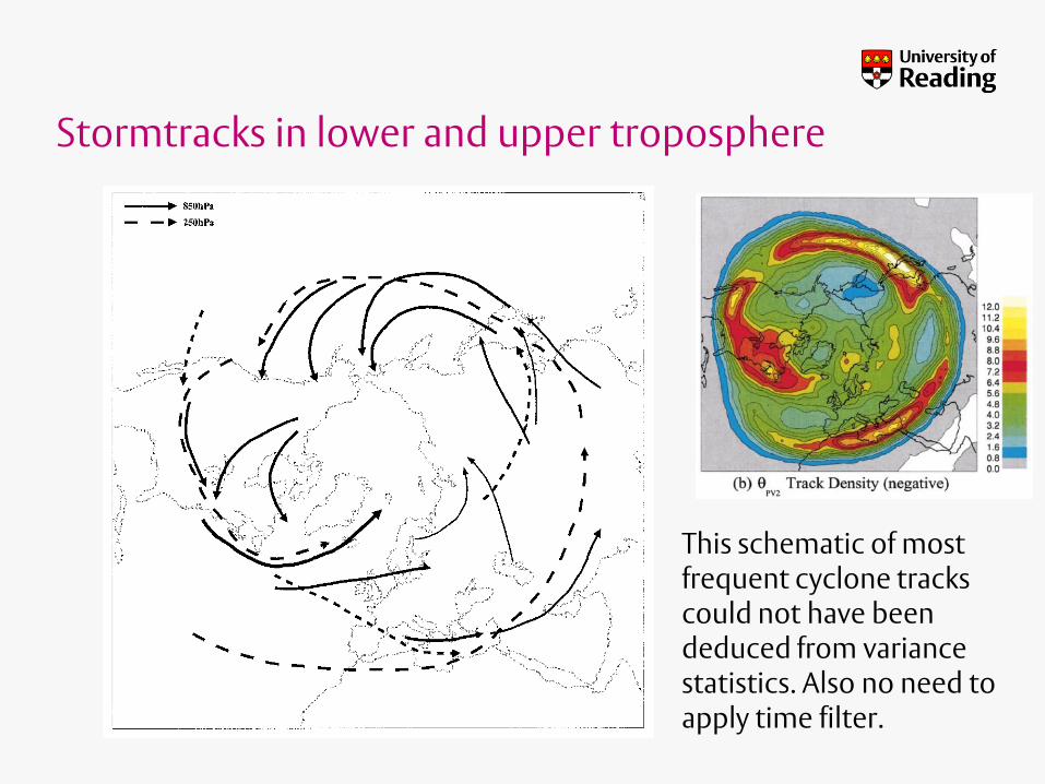
Stormtracks in lower and upper troposphere

This schematic of most frequent cyclone tracks could not have been deduced from variance statistics. Also no need to apply time filter.

Creating cyclone compositesDiagnosing climate model deficiencies

HiGEM climate model (version of UM)

ERA40 compositec

Jen Catto, Len Shaffrey and Kevin Hodges

Cyclone tracks in ensemble forecastsLizzie Froude, ESSC, submitted to Weather and Forecasting

Using Kevin Hodges’ cyclone tracking algorithm on ensemble forecasts from different centres archived on TIGGE database @ ECMWF.

Example of the control forecasts for one cyclone collated from 9 operational centres.

Bias in intensity and speed

Forecasts from most centres underestimate cyclone intensity (except ECMWF, CMA, CMC).

Cyclones propagate too slowly in forecasts (feature of all centres).

• Diagnosis of eddies and their effects on background flow depends

critically on method used to define background state.

• Modified Lagrangian Mean state seems like a better way forward

than Eulerian zonal or time average.

• Wave activity conservation laws provide crucial diagnostics of

Rossby wave packet propagation and teleconnections.

• Extreme seasons often related to persistent almost stationary

Rossby wave patterns (teleconnections). Can exist in the absence of

forcing, and Rossby wave “source” depends on wave, so cause and effect

becomes muddy.

• Cyclone tracking is valuable tool being used to evaluate models and

ensemble forecast skill.

3. Conclusions on mean flow and eddies

Summing up: Nature of the atmosphere

2. Balance and PV

• PV anomalies induce flow at-a-distance.

• Inversion to obtain vertical motion or overturning circulations is also non-local.

1. Transport

• Thermodynamic and chemical tracers carried vast distances

Complex source-receptor relationships.


• Waves forced in one location can propagate across globe and break/dissipate far away wave-transport.

• Eddies affect one another via the influence they have on the mean state.

Beware regional budgets: action-at-a-distance, wave propagation and mass transport all create complex interplay between a region and its surroudings.

Summing up: Suitable Diagnostics

2. Balance and PV

• PV as tracer and tracers for accumulated non-conservative effects

• PV error diagnostics

• Piecewise PV inversion and PV modification of forecasts

1. Transport

• Trajectories and tracer fields

• Advection-condensation models


• Equivalent latitude coordinates for tracer diagnostics.

Modified Lagrangian mean state

• Teleconnections, Rossby wave source and wave activity flux.

• Cyclone tracking and composite analysis.

John Methven, Department of Meteorology - ECMWF · John Methven, Department of Meteorology. ......

Documents

Transcript of John Methven, Department of Meteorology - ECMWF · John Methven, Department of Meteorology. ......