JHEP06(2020)085

Published for SISSA by Springer

Received: April 21, 2020

Accepted: May 19, 2020

Published: June 12, 2020

Islands in Schwarzschild black holes

Koji Hashimoto, Norihiro Iizuka and Yoshinori Matsuo

Department of Physics, Osaka University,

1-1 Machikaneyama, Toyonaka, Osaka 560-0043, Japan

E-mail: koji@phys.sci.osaka-u.ac.jp, iizuka@phys.sci.osaka-u.ac.jp,

matsuo@het.phys.sci.osaka-u.ac.jp

Abstract: We study the Page curve for asymptotically flat eternal Schwarzschild black

holes in four and higher spacetime dimensions. Before the Page time, the entanglement

entropy grows linearly in time. After the Page time, the entanglement entropy of a given

region outside the black hole is largely modified by the emergence of an island, which

extends to the outer vicinity of the event horizon. As a result, it remains a constant value

which reproduces the Bekenstein-Hawking entropy, consistent with the finiteness of the von

Neumann entropy for an eternal black hole.

Keywords: Black Holes, Black Holes in String Theory

ArXiv ePrint: 2004.05863

Open Access, c© The Authors.

Article funded by SCOAP3.https://doi.org/10.1007/JHEP06(2020)085

JHEP06(2020)085

Contents

1 Introduction and our strategy 1

2 No island, no entropy bound 6

3 Island saves the entropy bound 7

3.1 Close look at the black hole 7

3.2 View from a distance 8

4 Higher dimensions 10

5 Page time and scrambling time 12

A Early time growth of the entropy 15

B Geodesic distance and extremal volume 16

1 Introduction and our strategy

The information paradox [1] is the most fundamental problem in quantum gravity. The

Hawking radiation behaves as thermal radiation [2], which implies that the entanglement

entropy outside the black hole is monotonically increasing. On the other hand, quantum

mechanics requires that the entanglement entropy goes to zero at the end of the evapora-

tion since it must be the pure state. The time evolution of the entanglement entropy is

described by the so-called Page curve [3, 4]. Thus, the information loss paradox is trans-

lated to the problem how the Page curve is reproduced for the entanglement entropy of

the Hawking radiation.

Recently it was proposed that the Page curve emerges from the effect of islands [5–8].

Regarding the state of the Hawking radiation as that in a region R outside the black hole,

the density matrix of R is normally defined by taking the partial trace over the states in

R, which is the complementary region of R. According to the prescription of the minimal

quantum extremal surface [9–11], states in some regions in R, which are called islands

I(⊂ R), should be excluded from the states to be traced out. Thus, the entanglement

entropy of the Hawking radiation R is effectively given by that of states in R∪I. Explicitly,

the entanglement entropy of the Hawking radiation is give by

S(R) = min

ext

[Area(∂I)

4GN+ Smatter(R ∪ I)

], (1.1)

by using the prescription of the quantum extremal surface.

– 1 –

JHEP06(2020)085

The island rule was first proposed as a result of the conjectured quantum extremal

surface prescription, and recently the island rule was derived by using the replica method for

the gravitational path integral. When one applies the replica trick [14–16] to gravitational

theories, one can fix only the boundary conditions of the replica geometries, and new

saddles, where bulk wormholes are connecting different copies of spacetime, need to be

taken into account. These new saddles, called replica wormholes, lead to islands [12, 13].

In the semi-classical limit of gravity, the partition function of the geometry with replicas

is dominated by that giving the minimum entanglement entropy. In this way, the replica

trick for gravitational theories leads to the same formula (1.1) as the quantum extremal

surface prescription.

Since the replica wormhole is merely a consequence of the replica trick in models with

gravitation, the island conjecture is expected to be applicable to any black hole. So far,

among recent works [5–8, 12, 13, 17–27], the island rule has been studied mainly in two

spacetime dimensions,1 which offer a tractable treatment of the entanglement entropy of the

Hawking radiation. In this paper, we make one more step for general black holes. We study

the effect of islands in the Schwarzschild black holes, in asymptotically flat spacetime in

generic dimensions. Needless to say, the asymptotically flat four-dimensional Schwarzschild

black hole is the first solution historically [29] and the simplest and the most interesting

black hole. We start with the four-dimensional case.

The gravitational part of the action is given by the Einstein-Hilbert action with the

Gibbons-Hawking term,

I = Igravity + Imatter , (1.2)

Igravity =1

16πGN

∫Md4x√−g R+

1

8πGN

∫∂M

d3x√−hK , (1.3)

where GN is the Newton constant.2 Our goal in this paper is to show that the entanglement

entropy of the Hawking radiation of the Schwarzschild black hole follows a Page curve once

islands are taken into account. The Schwarzschild black hole metric we consider is

ds2 = − r − rh

rdt2 +

r

r − rhdr2 + r2dΩ2 (1.4)

with the horizon radius rh. Its temperature is

TH =1

β=

1

4πrh. (1.5)

In the following we summarize our analyses and necessary ingredients for them. First,

we will apply the quantum extremal surface (or equivalently, the replica wormhole) pre-

scription to gravity theory with matter fields. We do not resort to holographic correspon-

dences, nor to embedding into higher-dimensional (AdS) spacetime, nor to coupling with

an auxiliary system to absorb the radiation. We will use the global two-sided geometry.

1See ref. [28] for the study of islands in higher dimensions.2It is straightforward to generalize the analysis to gravity with higher curvature terms, but we focus

only on the dominant contributions.

– 2 –

JHEP06(2020)085

Before we proceed, we comment on the formula (1.1). The formula (1.1) consists of

two terms; the gravitational part3 of the generalized entropy, Sgravity, which is proportional

to the total area (or volume for D > 4) of the boundaries of an island, ∂I, as [30–33]

Sgravity =Area(∂I)

4GN, (1.6)

and the matter entanglement entropy Smatter on the region I and R in the curved back-

ground. Note that the formula given by eq. (1.6) is consistent with our action (1.3). Note

also that without islands, the gravitational entropy of an island, I, vanishes.

Unlike two-dimensions, in four-dimensions, it is well-known that the matter entangle-

ment entropy has area-like divergences, which depend on the short distance cut-off [36, 37].

Therefore, this yields the following divergence for the matter entropy

Smatter(R ∪ I) =Area(∂I)

ε2+ S

(finite)matter (R ∪ I) , (1.7)

where ε is the short distance cut-off scale.4 This divergence can be absorbed by the renor-

malization of the Newton constant as [38]

1

4G(r)N

=1

4GN+

1

ε2, (1.8)

where GN is bare Newton constant and G(r)N is renormalized Newton constant. In this

respect, if we regard GN in the formula (1.1) as the renormalized Newton constant, then

the leading cut-off dependent divergence of Smatter(R∪ I) in eq. (1.7) is already taken into

account, and therefore Smatter(R ∪ I) yields only a finite contribution, i.e. S(finite)matter (R ∪ I);

therefore our proposal formula in higher dimensions is

S(R) = min

ext

[Area(∂I)

4G(r)N

+ S(finite)matter (R ∪ I)

]. (1.9)

By evaluating the formula (1.9) as the prescription of the minimal quantum extremal

surface in higher dimensions, in this paper, we will derive the Page curve. For the finite

matter entropy contribution, S(finite)matter (R∪ I), we will use eq. (1.11) and eq. (1.12). This can

be understood as follows.

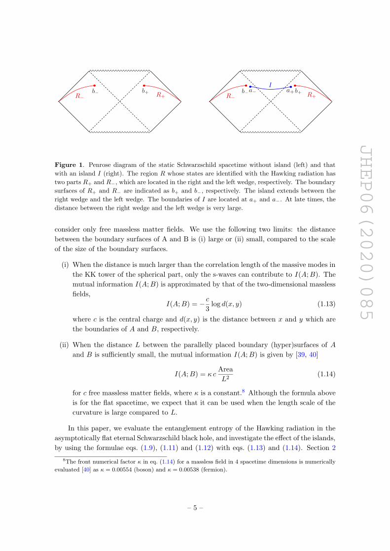
The region for the Hawking radiation R in the Schwarzschild spacetime is the union

of two regions R+ and R− which are located in the right and left wedges in the Penrose

diagram, respectively (see figure 1). The distance between R+ and R− becomes very large

at late times (see appendix B), therefore at late times, the entanglement entropy of the

Hawking radiation without islands is expected to be very large and the configuration with

islands is expected to give the dominant contribution.

3The gravitational part of the generalized entropy contains the term proportional to the area of ∂R. It

comes from the effect that the region R is separated from the other and is irrelevant to the entropy of the

Hawking radiation. In fact, it exists even in the case of the empty flat spacetime (without black holes) as

far as we consider bulk gravitational theories.4Similarly we have area-divergence coming from the boundary of R, which is irrelevant and we will

neglect in this paper.

– 3 –

JHEP06(2020)085

First, we consider the configuration without islands. The matter entanglement entropy

we will evaluate is that of separated two regions R+ and R− (see figure 1 Left). In this

case, the finite contributions of the matter entanglement entropy is, S(R+ ∪ R−) minus

S(R+)+S(R−), which is essentially the minus of the mutual information I(R+;R−).5 This

is because the leading contributions of the entanglement entropy of each region, S(R+)

and S(R−), are the divergences of the form (1.7), proportional to the area of the boundary

surface. Hence these cut-off dependent leading boundary-area divergences are already taken

into account by the renormalized Newton constant and do not contribute to S(finite)matter (R∪I).6

Thus, in the case of no island, the finite part of the matter entanglement entropy is given

in terms of the mutual entropy as

S(finite)matter (R ∪ I) = S

(finite)matter (R) = −I(R+;R−) (without island) (1.11)

Next, we consider the configuration with an island I. At late times, each of two

boundaries of I is much closer to the boundary of R in the same wedge, than to the

boundaries of R and I in the other wedge (see figure 1 Right).7 The correlation between

the left and right wedges is negligible since the neighboring boundary (hyper)surfaces

of different regions behaves like charges with opposite sign. Thus the total entanglement

entropy is well dominated by that in each side separately. In fact, in the case with an island,

a symmetric configuration will give the minimal entropy. We may consider only the right

wedge, since the contributions from the right and left wedges will be equal to each other, so

in total it is twice of the contribution of only the right wedge. The finite contributions of the

matter entanglement entropy from only the right wedge is S(R+ ∪ I) minus S(R+) +S(I),

which is essentially the minus of the mutual information I(R+; I). Therefore, in the case

with an island, the finite part of the matter entanglement entropy is given as

S(finite)matter (R ∪ I) = −2I(R+, I) (with an island I) (1.12)

In this paper, for the finite matter entropy contribution, S(finite)matter (R ∪ I) for eq. (1.9), we

use eq. (1.11) and eq. (1.12).

The generic expression for the mutual information I(A;B) in curved spacetimes is not

known, so we need to make some assumptions and take some limits. In this paper, we

5The mutual information I(A;B) is given by,

I(A;B) ≡ −S(A ∪B) + S(A) + S(B) . (1.10)

6There are higher order corrections to the area terms of the entanglement entropy, which are also

renormalized into the higher order gravitational constants.7The distance between the right and the left boundaries is characterized by the volume of an extremal

surface connecting the boundaries. The calculation of that extremal surface resembles that of a holographic

complexity (“complexity = volume” conjecture [34, 35]). As shown in appendix B, at late times, the

volume of the three-dimensional extremal surface in the analytically continued Schwarzschild geometry

grows linearly in time. The section of this extremal surface is at most 4πb2 where b is the value of the radial

coordinate of the Schwarzschild geometry, thus the extremal three-dimensional surface is a long cylinder

at late times. This means that the four-dimensional matter free fields can be treated as a two-dimensional

massless fields which are the lowest mode in the KK towers.

– 4 –

JHEP06(2020)085

b+<latexit sha1_base64="(null)">(null)</latexit><latexit sha1_base64="(null)">(null)</latexit><latexit sha1_base64="(null)">(null)</latexit><latexit sha1_base64="(null)">(null)</latexit>

b<latexit sha1_base64="(null)">(null)</latexit><latexit sha1_base64="(null)">(null)</latexit><latexit sha1_base64="(null)">(null)</latexit><latexit sha1_base64="(null)">(null)</latexit>

R+<latexit sha1_base64="(null)">(null)</latexit><latexit sha1_base64="(null)">(null)</latexit><latexit sha1_base64="(null)">(null)</latexit><latexit sha1_base64="(null)">(null)</latexit>

R<latexit sha1_base64="(null)">(null)</latexit><latexit sha1_base64="(null)">(null)</latexit><latexit sha1_base64="(null)">(null)</latexit><latexit sha1_base64="(null)">(null)</latexit>

b+<latexit sha1_base64="(null)">(null)</latexit><latexit sha1_base64="(null)">(null)</latexit><latexit sha1_base64="(null)">(null)</latexit><latexit sha1_base64="(null)">(null)</latexit>

b<latexit sha1_base64="(null)">(null)</latexit><latexit sha1_base64="(null)">(null)</latexit><latexit sha1_base64="(null)">(null)</latexit><latexit sha1_base64="(null)">(null)</latexit>

a<latexit sha1_base64="(null)">(null)</latexit><latexit sha1_base64="(null)">(null)</latexit><latexit sha1_base64="(null)">(null)</latexit><latexit sha1_base64="(null)">(null)</latexit> a+<latexit sha1_base64="(null)">(null)</latexit><latexit sha1_base64="(null)">(null)</latexit><latexit sha1_base64="(null)">(null)</latexit><latexit sha1_base64="(null)">(null)</latexit>

I<latexit sha1_base64="(null)">(null)</latexit><latexit sha1_base64="(null)">(null)</latexit><latexit sha1_base64="(null)">(null)</latexit><latexit sha1_base64="(null)">(null)</latexit>

R+<latexit sha1_base64="(null)">(null)</latexit><latexit sha1_base64="(null)">(null)</latexit><latexit sha1_base64="(null)">(null)</latexit><latexit sha1_base64="(null)">(null)</latexit>

R<latexit sha1_base64="(null)">(null)</latexit><latexit sha1_base64="(null)">(null)</latexit><latexit sha1_base64="(null)">(null)</latexit><latexit sha1_base64="(null)">(null)</latexit>

Figure 1. Penrose diagram of the static Schwarzschild spacetime without island (left) and that

with an island I (right). The region R whose states are identified with the Hawking radiation has

two parts R+ and R−, which are located in the right and the left wedge, respectively. The boundary

surfaces of R+ and R− are indicated as b+ and b−, respectively. The island extends between the

right wedge and the left wedge. The boundaries of I are located at a+ and a−. At late times, the

distance between the right wedge and the left wedge is very large.

consider only free massless matter fields. We use the following two limits: the distance

between the boundary surfaces of A and B is (i) large or (ii) small, compared to the scale

of the size of the boundary surfaces.

(i) When the distance is much larger than the correlation length of the massive modes in

the KK tower of the spherical part, only the s-waves can contribute to I(A;B). The

mutual information I(A;B) is approximated by that of the two-dimensional massless

fields,

I(A;B) = − c3

log d(x, y) (1.13)

where c is the central charge and d(x, y) is the distance between x and y which are

the boundaries of A and B, respectively.

(ii) When the distance L between the parallelly placed boundary (hyper)surfaces of A

and B is sufficiently small, the mutual information I(A;B) is given by [39, 40]

I(A;B) = κ cArea

L2(1.14)

for c free massless matter fields, where κ is a constant.8 Although the formula above

is for the flat spacetime, we expect that it can be used when the length scale of the

curvature is large compared to L.

In this paper, we evaluate the entanglement entropy of the Hawking radiation in the

asymptotically flat eternal Schwarzschild black hole, and investigate the effect of the islands,

by using the formulae eqs. (1.9), (1.11) and (1.12) with eqs. (1.13) and (1.14). Section 2

8The front numerical factor κ in eq. (1.14) for a massless field in 4 spacetime dimensions is numerically

evaluated [40] as κ = 0.00554 (boson) and κ = 0.00538 (fermion).

– 5 –

JHEP06(2020)085

shows that the entropy without the island grows linearly in time at late times. In section 3

we include the island and the extremization about the location of it results in the time-

independent behavior of the entropy. We treat two cases: section 3.1 for the entanglement

region R close to the horizon, and section 3.2 for R far away from the horizon. Both

cases show that the emergent island extends to the outer vicinity of the horizon, and the

total entropy at late times is almost twice the Bekenstein-Hawking entropy formula. For

simplicity the calculations are given for D = 4 spacetime dimensions, and in section 4 we

show that all results are qualitatively the same in generic higher dimensions. Finally in

section 5 we draw the Page curve and discuss the Page time and the scrambling time. From

now on, we write the renormalized Newton constant simply as GN.

2 No island, no entropy bound

In this section we evaluate the entanglement entropy at late times, in the case of the

absence of the island. For the two-dimensional s-wave approximation to make sense, all

the points in eq. (1.13) need to be well-separated, compared to the scale of the radius of

the sphere. In the absence of the island, we have only two points which are the boundaries

of the entanglement regions at the right R and the left R (see figure 1 Left). So, at late

time, we can use the formulas (1.11) and (1.13) as

Smatter =c

3log d(b+, b−) (2.1)

where b+ and b− stand for the boundaries of the entanglement regions in the right and

the left wedges of the Schwarzschild geometry. Here (t, r) = (tb, b) for b+ and (t, r) =

(−tb + iβ/2, b) for b−, respectively.9 Following a conformal map, we find that the matter

part of the entanglement entropy in the Schwarzschild geometry is

Smatter =c

6log

(U(b−)− U(b+)) (V (b+)− V (b−))

W (b+)W (b−). (2.2)

Here the Schwarzschild metric in the Kruskal coordinates is given by

ds2 = −dUdVW 2

+ r2dΩ2 , (2.3)

where we have defined the coordinates as

r∗ = r − rh + rh logr − rh

rh, (2.4)

U ≡ −e−t−r∗2rh = −

√r − rh

rhe− t−(r−rh)

2rh , V ≡ et+r∗2rh =

√r − rh

rhet+(r−rh)

2rh . (2.5)

The conformal factor W of the Schwarzschild black hole geometry is

W =

√r

4rh

UV

r − rh=

√r

4r3h

er−rh2rh . (2.6)

9The imaginary part iβ/2 of time t implies that it is in the left wedge, which means that U and V in

the Kruskal coordinates have extra minus sign, as seen in the following.

– 6 –

JHEP06(2020)085

Then, the total entanglement entropy is calculated as

S =c

6log

[16r2

h(b− rh)

bcosh2 tb

2rh

]. (2.7)

As we mentioned the two-dimensional approximation is valid for late time, tb b (>

rh), so the above result is approximated as

S ' c

6

tbrh, (2.8)

which grows linearly in time.

At the late times wherec t

rh

r2h

GN, (2.9)

this entropy becomes much larger than the black hole entropy. This contradicts with the

finiteness of the von Neumann entropy for a finite-dimensional black hole system. In such

a case, an island is expected to emerge. In the next section, we calculate the entanglement

entropy with a single island and show that in fact the Page curve is reproduced once we

take into account the effects of an island.

3 Island saves the entropy bound

In this section we calculate the entanglement entropy with a single island. The configura-

tion is shown in figure 1 Right. To capture the entropy of the full degrees of freedom of

the radiation, the entanglement region R had better be close to the event horizon. So first

we consider such a case of looking at the black hole closely, b − rh rh, in section 3.1.

Then later in section 3.2 we consider the other case when the boundary of the region R is

far away from the horizon, that is, a view from a distance.

3.1 Close look at the black hole

Let us consider the case b − rh rh, the close look at the black hole from the region

R. The boundaries of the island I, a±, are located at (t, r) = (ta, a) for a+ and (t, r) =

(−ta + iβ/2, a) for a−. It is plausible that ta = tb would extremize the entropy, and in

this subsection we assume it. We also assume that at late times, due to the fact that the

left wedge and the right wedge are separated by the volume growing linear in time (see

appendix B), we just need to focus on the right-hand side of the Penrose diagram for the

calculation of the entropy (and the final result is twice of it). Then the total entropy is

S ' 2πa2

GN− 2κc

4πb2

L2, (3.1)

where the distance between the end point of the island I and that of the entanglement

region R is the geodesic distance,

L =

∫ b

a

dr√1− rh

r

. (3.2)

– 7 –

JHEP06(2020)085

We need to extremize the entropy with respect to a which is the location of the bound-

ary of the island. Physically, when we regard the entropy S as a potential energy for a

particle located at r = a, this extremization is due to the harmonic (gravitational) poten-

tial 2πa2

GNand the attractive potential −2κc4πb2

L2 which pushes the particle closer to r = b.

The entropy formula (1.14) is valid only if L a, which is fine because we here consider

the case b− rh rh (and resultantly a− rh rh).

In that case, the geodesic distance (3.2) is

L ' 2√rh

(√b− rh −

√a− rh

). (3.3)

To minimize the entropy (3.1) with respect to a, we change the variable to x ≡√

a−rhrh

,

and consider the equation ∂S∂x = 0 which is equivalent to

x

(√b− rh

rh− x

)3

=κcGN

2r2h

, (3.4)

where approximations x 1 and b ≈ rh are taken into account. This equation has at most

two solutions for x. The minimization occurs at a smaller x solution, satisfying x√

b−rhrh

,

and with the fact that the right-hand side of eq. (3.4) is very small, we find the location of

the island as

a = rh +(κcGN)2

4(b− rh)3. (3.5)

So the boundary of the island is located very close to, and slightly outside of, the black

hole horizon.

Substituting this expression to the total entropy, we find

S =2πr2

h

GN− 2πκ c

rh

b− rh. (3.6)

We find a very natural interpretation of this result. First of all, this is constant, as opposed

to the late time result without the island, eq. (2.8). Therefore, the configuration with the

island is preferred, and the entropy stops growing at late times. The first term in eq. (3.6)

is exactly (twice of) the Bekenstein-Hawking entropy formula [2, 41]. The second term is

the effect of the quantum matter.

3.2 View from a distance

Next, let us consider the case when the boundary r = b of the entanglement region R is

far away from the horizon, b rh. In this case, we assume that the s-wave approximation

is valid,10 and use the matter entropy formula (1.13) for calculating the total entropy.

10The length scale of the angular sphere at r = b is b, while the distance between a (> rh) to b is smaller

than b. So this would cause a problem for adopting the two-dimensional formula (1.13). Here, since the

Hawking radiation observed at an asymptotic observer is dominated by the s-wave, we assume the use of

the two-dimensional formula (1.13).

– 8 –

JHEP06(2020)085

The entanglement entropy for the conformal matter is given by

Smatter =c

3log

d(a+, a−)d(b+, b−)d(a+, b+)d(a−, b−)

d(a+, b−)d(a−, b+). (3.7)

Using the Kruskal coordinates given in section 2, the total entanglement entropy is calcu-

lated as

S =2πa2

GN+c

6log

[28r4

h(a− rh)(b− rh)

abcosh2 ta

2rhcosh2 tb

2rh

]

+c

3log

cosh(r∗(a)−r∗(b)

2rh

)− cosh

(ta−tb2rh

)cosh

(r∗(a)−r∗(b)

2rh

)+ cosh

(ta+tb2rh

) , (3.8)

where

coshr∗(a)− r∗(b)

2rh=

1

2

[√a− rh

b− rhea−b2rh +

√b− rh

a− rheb−a2rh

]. (3.9)

The island is expected to show up near the black hole horizon, so we assume a ∼ rh and

check if this approximation is correct or not, later. For a ∼ rh, the second term in the

right-hand side of eq. (3.9) dominates, so we ignore the first term.

Let us consider the late time behavior. We take the late time approximation11

1

2

√b− rh

a− rheb−a2rh cosh

ta + tb2rh

. (3.10)

We also consider the approximation

coshta − tb

2rh 1

2

√b− rh

a− rheb−a2rh (3.11)

which will be checked to be satisfied later. Then the entanglement entropy (3.8) is approx-

imated as12

S =2πa2

GN+c

6log

[28r4

h(a− rh)(b− rh)

abcosh2 ta

2rhcosh2 tb

2rh

]− c

3log

[1

2

√a− rh

b− rhea−b2rh cosh

ta + tb2rh

]− 2c

3

√a− rh

b− rhea−b2rh cosh

ta − tb2rh

=2πa2

GN+c

6log

[16r4

h(b− rh)2

abeb−arh

]− 2c

3

√a− rh

b− rhea−b2rh cosh

ta − tb2rh

. (3.14)

11In appendix A, we study the early time behavior and find that there is no saddle point for the location

of the island, meaning that the island is not generated.12At late times, the distance between the right wedge and the left wedge is very large, so we have

d(b+, b−) ' d(a+, a−) ' d(b±, a∓) d(b±, a±) , (3.12)

and the entanglement entropy of the matter is approximated as

Smatter =c

3log [d(a+, b+)d(a−, b−)] . (3.13)

This simplified expression indeed results in the expression same as eq. (3.14).

– 9 –

JHEP06(2020)085

This allows a local minimum at

a ' rh +(cGN)2

144π2r2h(b− rh)

erh−brh cosh2 ta − tb

2rh, (3.15)

and with that value of a the total entropy (3.14) is calculated as

S =2πr2

h

GN+c

6log

[16r3

h(b− rh)2

beb−rhrh

]− c2GN

36πrh(b− rh)erh−brh cosh2 ta − tb

2rh. (3.16)

We vary this expression for ta and find that ta = tb extremizes it. For ta = tb, the value of a

given in eq. (3.15) in fact satisfies eq. (3.11). The late time condition (3.10) is rewritten as

rh logrh(b− rh)

cGN tb . (3.17)

Then in eq. (3.16) we put ta = tb and ignore higher order terms in GN, to obtain the final

expression of the entanglement entropy

S =2πr2

h

GN+c

6

[log

(16r3

h(b− rh)2

b

)+b− rh

rh

]. (3.18)

This does not grow in time. The interpretation of this result is the same as in the result of

the close look, eq. (3.6). The first term, which emerged as a result of the island, provides

the Bekenstein-Hawking entropy formula [2, 41] for the four-dimensional Schwarzschild

black hole.

So summarizing the close look result (3.6) and the distant look result (3.18), we have

confirmed that the island shows up at late times and the entropy growth disappears. The

boundary of the island is located very close to the event horizon, and in fact the island

provides the renowned Bekenstein-Hawking entropy of the Schwarzschild black hole.

4 Higher dimensions

The arguments presented in this paper can go through for the case of Schwarzschild black

holes in higher spacetime dimensions, D ≥ 4. In this section, we provide results in generic

D dimensions, and find that the results obtained in section 2 and section 3 are universal.

The Schwarzschild metric in D dimensions is

ds2 = −f(r)dt2 +dr2

f(r)+ r2dΩ2

D−2 , f(r) ≡ 1−rD−3

h

rD−3. (4.1)

The area of the (D− 2)-sphere at radius r is rD−2ΩD−2, where ΩD−2 is the volume of the

unit (D − 2)-sphere.

First, we look at the case with no island. Similarly to section 2, the Kruskal coordinates

are given13 just by generalizing the factor f(r). We arrive at the expression for the total

entropy at late times,

S ' c

6(D − 3)

tbrh. (4.4)

13The Kruskal coordinates in the right wedge are

U ≡ − exp

[−(D − 3)

t− r∗2rh

], V ≡ exp

[(D − 3)

t+ r∗2rh

], (4.2)

– 10 –

JHEP06(2020)085

For D = 4 this reproduces eq. (2.8). There is no physical difference; the entropy grows

linearly in time.

Next, we consider the entanglement entropy with the island. For the close look at

the black hole as in section 3.1, instead of the four-dimensional formula (1.14), we use the

D-dimensional formula

I(A;B) = κD cArea

LD−2. (4.5)

Here the constant κD also depends on D. The total entropy with the island contribution is

S ' ΩD−2

2GNaD−2 − 2κD c

ΩD−2 bD−2

LD−2(4.6)

with the distance in the short distance approximation b, a ' rh,

L ' 2√D − 3

√rh

(√b− rh −

√a− rh

). (4.7)

We minimize S by varying the location a of the boundary of the island, and find

a = rh +(κD cGN)2

r2D−5h

26−2D(D − 3)D−2

(rh

b− rh

)D−1

. (4.8)

So the island is located very close to the black hole horizon. The total entanglement entropy

is found as

S =ΩD−2

2GNrD−2

h − ΩD−2κD c 23−D(D − 3)(D−2)/2

(rh

b− rh

)(D−2)/2

. (4.9)

This reproduces eq. (3.6) for D = 4. Again, the contribution of the Bekenstein-Hawking

entropy emerges as the island contribution, and there exists a small contribution from the

matter field (the second term).

We can also work out the higher dimensional case for the view at a distance given in

section 3.2. The total entanglement entropy with the island at late times is

S ' ΩD−2

2GNaD−2 +

c

6

[log

[24r4

hf(b)f(a)

(D − 3)4

]+ 2(D − 3)

r∗(b)− r∗(a)

2rh

]− 2c

3exp

[(D − 3)

r∗(a)− r∗(b)2rh

]cosh

[(D − 3)

ta − tb2rh

]. (4.10)

The location of the boundary of the island is again found to be very close to the horizon,

a = rh +(cGN)2

r2D−5h

(2

3(D−2)ΩD−2

)2

exp

[(3−D)

(b

rh−1+g

(b

rh

))]cosh2

[(D−3)

ta − tb2rh

],

(4.11)

with r∗ ≡∫ rdr/f(r), giving the metric of the form (2.3) with

W ≡ (D − 3)

2rh√f(r)

exp

[(D − 3)

r∗2rh

]. (4.3)

– 11 –

JHEP06(2020)085

where we have defined14

g(x)≡−x4−D

D−42F1

(1,D−4

D−3,

2D−7

D−3;x3−D

)− 1

D−3

(γ+log(D−3)+

Γ′((D−4)/(D−3))

Γ((D−4)/(D−3))

).

Substituting eq. (4.11) to the total entropy, we find again ta = tb extremizes it, and the

final expression for the entanglement entropy is

S ' ΩD−2

2GNrD−2

h +c

6

[log

[24r4

hf(b)

(D−3)3

]+ (D−3)

(b

rh−1+g

(b

rh

))]. (4.12)

The first term of this late-time expression of the entanglement entropy is the Bekenstein-

Hawking entropy which emerged from the island. This eq. (4.12) shares the same structure

as eq. (4.9).

5 Page time and scrambling time

In this paper, we have calculated the entanglement entropy of the Hawking radiation of the

asymptotically flat eternal Schwarzschild black hole in D (≥ 4) spacetime dimensions, for

the configuration without islands and that with an island. We can summarize the findings,

eqs. (2.8), (4.4), (3.6), (3.18), (4.9), and (4.12), as follows. The entanglement entropy of

a given region R outside of the horizon linearly grows with time t for the configuration

without islands;

S =c

6(D − 3)

t

rh, (5.1)

where rh is the Schwarzschild radius and c is the number of massless matter fields. For the

case with an island at late times, the saddle point analysis for the boundary of the island

a shows that it emerges at the outer vicinity of the horizon,

a = rh +O

((cGN)2

r2D−5h

). (5.2)

The resultant entanglement entropy for the region R is15

S = 2SBH +O(c) , (5.3)

where SBH is the Bekenstein-Hawking entropy of the Schwarzschild black hole, SBH ≡Area(r = rh)/4GN, which is time-independent at late times. O(c) effects arise from the

quantum effects by the matters.

Generally, the dominant contribution to the entanglement entropy comes from the con-

figuration with a minimum entropy. Thus, for the eternal Schwarzschild black holes, at early

14The function g(x) reduces to log(x− 1) at D = 4. The complicated form of g(x) is just because of the

Kruskal coordinates in higher dimensions.15In this paper we have assumed the dimensionless quantity cGN/r

D−2h 1. This applies to our universe,

since the number of massless fields c is not very large, while the Newton constant GN, or equivalently, the

Planck length is much smaller than the typical scale of realistic black holes. Therefore, the higher order

terms in eq. (5.2) and similar expressions are negligible.

– 12 –

JHEP06(2020)085

t<latexit sha1_base64="(null)">(null)</latexit><latexit sha1_base64="(null)">(null)</latexit><latexit sha1_base64="(null)">(null)</latexit><latexit sha1_base64="(null)">(null)</latexit>

S<latexit sha1_base64="(null)">(null)</latexit><latexit sha1_base64="(null)">(null)</latexit><latexit sha1_base64="(null)">(null)</latexit><latexit sha1_base64="(null)">(null)</latexit>

0<latexit sha1_base64="(null)">(null)</latexit><latexit sha1_base64="(null)">(null)</latexit><latexit sha1_base64="(null)">(null)</latexit><latexit sha1_base64="(null)">(null)</latexit>

2SBH<latexit sha1_base64="3DpQsgfPoG+Y/PQUuPdo8PrXNAY=">AAACbnichVHLSsNAFD2Nr1pfVUEEEYtFcVUmVVFciW5cqrVVaEtJ4lRD8yKZFmrxB9yLC0FREBE/w40/4MJPEDdCBTcuvEkDoqLeMJkzZ+65c+aO6hi6Jxh7jEht7R2dXdHuWE9vX/9AfHAo59lVV+NZzTZsd0dVPG7oFs8KXRh8x3G5YqoG31Yrq/7+do27nm5bW6Lu8KKp7Fl6WdcUQVQ+nSk1Cq6ZWFk7LMWTLMWCSPwEcgiSCGPdjl+jgF3Y0FCFCQ4LgrABBR59echgcIgrokGcS0gP9jkOESNtlbI4ZSjEVui/R6t8yFq09mt6gVqjUwwaLikTmGIP7IY12T27ZU/s/ddajaCG76VOs9rScqc0cDSaeftXZdIssP+p+tOzQBmLgVedvDsB499Ca+lrByfNzNLmVGOaXbJn8n/BHtkd3cCqvWpXG3zzFDF6APl7u3+CXDolz6bmN+aSyyvhU0QxhknMUL8XsIw1rCMbdOwYZziPvEgj0rg00UqVIqFmGF9CmvkAE6eNrA==</latexit>

tPage<latexit sha1_base64="fZwSt3NTB4OYv5pJ4u+6AGbzQuY=">AAACb3ichVHLSgMxFD0dX7W+qi4UBCmWim5K6gPFVdGNyz6sClbKzBjr0HkxkxZq6Q/4Abpw4QNExM9w4w+46CeIK6ngxoW30wHRot6Q5OTknpuTRLF1zRWMNQJSV3dPb1+wPzQwODQ8Eh4d23atsqPynGrplrOryC7XNZPnhCZ0vms7XDYUne8opY3W/k6FO65mmVuiavN9Qy6a2qGmyoKovCjU8o4RSclFXi+EoyzOvIh0goQPovAjZYVvkccBLKgowwCHCUFYhwyX2h4SYLCJ20eNOIeQ5u1z1BEibZmyOGXIxJZoLNJqz2dNWrdqup5apVN06g4pI4ixJ3bHmuyR3bNn9vFrrZpXo+WlSrPS1nK7MHIymX3/V2XQLHD0pfrTs8AhVj2vGnm3PaZ1C7WtrxyfNbNrmVhtll2zF/J/xRrsgW5gVt7UmzTPnCNEH5D4+dydYHshnliML6eXosl1/yuCmMIM5ui9V5DEJlLI0bk2TnGBy8CrNCFNS5F2qhTwNeP4FtL8JwSKjpg=</latexit>

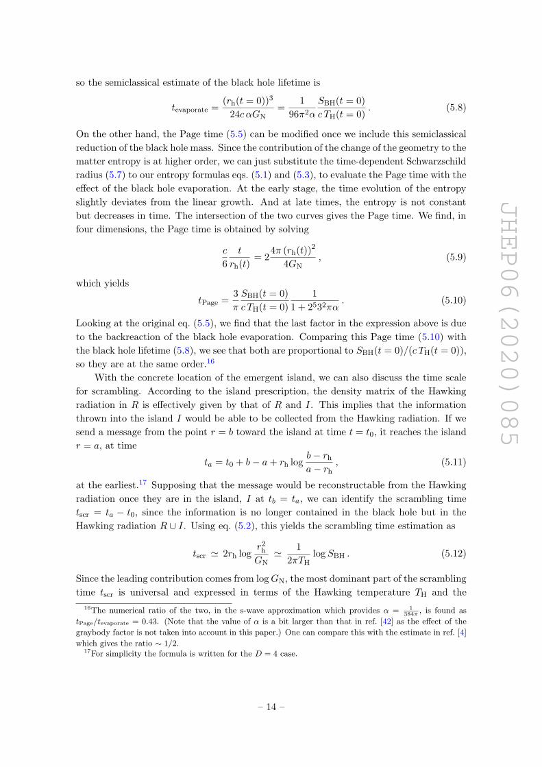
Figure 2. The Page curve for the eternal Schwarzschild black hole. In this plot we ignore terms of

higher order in cGN/rD−2h , which are small compared to tPage or SBH.

times the entanglement entropy is given by that of the configuration without the island,

then at late times it is by the one with the island. So the dominant configurations switch at

the time identified with Page time tPage, at which the time evolution of the entanglement

entropy drastically changes: the linear growth is replaced by a time-independent constant,

see figure 2. Equating the asymptotic constant value of the entropy (5.3) with the entropy

without the island (4.4), we find the Page time for the eternal Schwarzschild black hole,

tPage =3ΩD−2

(D − 3)

rD−1h

cGN+O (rh) . (5.4)

Although the higher order corrections would depend on b, which is the boundary location of

the entanglement region R, the leading term is universal. Using the Hawking temperature

TH = (D−3)4πrh

, the universal term is written as

tPage =3

π

SBH

c TH. (5.5)

After the Page time, the entropy is given by 2SBH for the Hawking radiation in the both

sides of the Penrose diagram. Thus the entanglement entropy for the Hawking radiation

observed only in a single side approximately agrees with SBH, as expected.

Let us compare the Page time with a semiclassical estimate of the lifetime of the black

hole [42]. In four dimensions, the radiation power reduces the mass M of the black hole as

dM

dt= − cα

G2NM

2(5.6)

where α is a constant dependent on the spin of the radiating particle. Solving this gives a

time-dependent Schwarzschild radius as

rh(t) = rh(t = 0)

[1− 24cα

GN t

(rh(t = 0))3

]1/3

, (5.7)

– 13 –

JHEP06(2020)085

so the semiclassical estimate of the black hole lifetime is

tevaporate =(rh(t = 0))3

24c αGN=

1

96π2α

SBH(t = 0)

c TH(t = 0). (5.8)

On the other hand, the Page time (5.5) can be modified once we include this semiclassical

reduction of the black hole mass. Since the contribution of the change of the geometry to the

matter entropy is at higher order, we can just substitute the time-dependent Schwarzschild

radius (5.7) to our entropy formulas eqs. (5.1) and (5.3), to evaluate the Page time with the

effect of the black hole evaporation. At the early stage, the time evolution of the entropy

slightly deviates from the linear growth. And at late times, the entropy is not constant

but decreases in time. The intersection of the two curves gives the Page time. We find, in

four dimensions, the Page time is obtained by solving

c

6

t

rh(t)= 2

4π (rh(t))2

4GN, (5.9)

which yields

tPage =3

π

SBH(t = 0)

c TH(t = 0)

1

1 + 2532πα. (5.10)

Looking at the original eq. (5.5), we find that the last factor in the expression above is due

to the backreaction of the black hole evaporation. Comparing this Page time (5.10) with

the black hole lifetime (5.8), we see that both are proportional to SBH(t = 0)/(c TH(t = 0)),

so they are at the same order.16

With the concrete location of the emergent island, we can also discuss the time scale

for scrambling. According to the island prescription, the density matrix of the Hawking

radiation in R is effectively given by that of R and I. This implies that the information

thrown into the island I would be able to be collected from the Hawking radiation. If we

send a message from the point r = b toward the island at time t = t0, it reaches the island

r = a, at time

ta = t0 + b− a+ rh logb− rh

a− rh, (5.11)

at the earliest.17 Supposing that the message would be reconstructable from the Hawking

radiation once they are in the island, I at tb = ta, we can identify the scrambling time

tscr = ta − t0, since the information is no longer contained in the black hole but in the

Hawking radiation R ∪ I. Using eq. (5.2), this yields the scrambling time estimation as

tscr ' 2rh logr2

h

GN' 1

2πTHlogSBH . (5.12)

Since the leading contribution comes from logGN, the most dominant part of the scrambling

time tscr is universal and expressed in terms of the Hawking temperature TH and the

16The numerical ratio of the two, in the s-wave approximation which provides α = 1384π

, is found as

tPage/tevaporate = 0.43. (Note that the value of α is a bit larger than that in ref. [42] as the effect of the

graybody factor is not taken into account in this paper.) One can compare this with the estimate in ref. [4]

which gives the ratio ∼ 1/2.17For simplicity the formula is written for the D = 4 case.

– 14 –

JHEP06(2020)085

Bekenstein-Hawking entropy SBH. This expression is valid in general dimensions, D ≥ 4.

The scrambling time obtained is proportional to 1/TH logSBH, as predicted first in ref. [43].

Several comments are in order. In this paper, we have studied only the configuration

without islands and that with an island. Configurations with more islands also might

contribute to the entanglement entropy. As the configuration with a single island agrees

with the entropy of the black hole, those with more islands would not have dominant

contributions at late times. They would contribute around the Page time, so that the

sharp change of the time evolution of the entanglement entropy may be smoothed away.

One remaining problem, which is important in the viewpoint of information, is how

the information in the island is transported to the Hawking radiation. We have found that

the expected Page curve is reproduced by the effect of the island, and the entanglement

entropy of the Hawking radiation agrees with that of the black hole. However these do

not tell how the information is restored concretely. Further study of islands will reveal the

mystery of the black hole information paradox.

Acknowledgments

K. H. would like to thank Sotaro Sugishita for discussions on ref. [44]. N. I. would like to

thank Takanori Anegawa for various helpful discussions on related project [27]. This work

is supported in part by JSPS KAKENHI Grant Number JP17H06462 (K.H.), JP18K03619

(N.I.).

A Early time growth of the entropy

In this appendix we study the early time growth of the entanglement entropy. At the very

early stage of the time evolution, the geodesic distance between the two points is short

compared to the scale of the area, so we can use the short distance formula (1.14).

In the formula (1.14) the separation L between the two regions R is approximated by

the geodesic distance in two-dimensional part of the Schwarzschild spacetime. At the short

distance expansion it should coincide18 with d in section 2,

L ' 4rh

√b− rh

rhcosh

t

2rh. (A.1)

For this L to be smaller than the scale of the area ∼ r2h, we need t rh log rh

b−rh and thus

b− rh rh.

Substituting eq. (A.1) to eq. (1.14), we find the total entropy,

S = − π2κc

4(brh− 1)

cosh2 t2rh

. (A.2)

This grows as ∼ t2 at early time 0 ≤ t rh log rhb−rh .

18We check indeed it coincides, see appendix B.

– 15 –

JHEP06(2020)085

So, together with the result given in section 2, we find that the total entanglement

entropy grows in time, when we do not include the contribution from the island. At early

times it grows as t2, and at late times it grows linearly in time.

Now, let us consider if we need to include the contribution from the island, at early

times. We look at the early time behavior of eq. (3.8).19 Suppose

1

2

√b− rh

a− rheb−a2rh cosh

ta + tb2rh

, coshta − tb

2rh(A.3)

which is valid at early times, ta, tb rh. The entanglement entropy (3.8) is approximated

as

S =2πa2

GN+c

6log

[28r4

h(a− rh)(b− rh)

abcosh2 ta

2rhcosh2 tb

2rh

]− 4c

3

√a− rh

b− rhea−b2rh cosh

ta2rh

coshtb

2rh. (A.4)

The location of the boundary of the island, r = a, is determined by minimization of

eq. (A.4). However, we find no saddle point, as seen in the following way. Writing a-

dependent terms in eq. (A.4) by x ≡√

(a− rh)/rh, eq. (A.4) is roughly written as

S ∼r2

h

GNx2 + c log x− cx . (A.5)

So, the saddle point equation has the structure

0 =∂S

∂x=

r2h

GNx+

c

x− c . (A.6)

For GNc/r2h 1, this does not allow a solution for x. Since there is no minimum for the

entropy as we vary a, we conclude that at early times the island is not generated.

B Geodesic distance and extremal volume

In appendix A, we have argued that the length scale d used in section 2 is equal to the sep-

aration L between the two regions R, given by the geodesic distance in the two-dimensional

part of the Schwarzschild spacetime,

L =

∫dt

√−(

1− rh

r

)+(

1− rh

r

)−1r2 . (B.1)

Here we show that it is indeed the case.

By integrating the equation of motion of eq. (B.1), or equivalently, since the Hamilto-

nian must be constant, we obtain a conservation law

λ =(1− rh

r )√−(1− rh

r

)+(1− rh

r

)−1r2

, (B.2)

19For the two-dimensional approximation to work, the geodesic distance between a− and a+ needs to be

large compared to rh. Looking at the formula (A.1), this means cosh ta √

a−rhrh

. When a is close enough

to rh, this is satisfied for any ta.

– 16 –

JHEP06(2020)085

where λ is a constant. By solving eq. (B.2), we find dt/dr as

dt

dr=

1(1− rh

r

)√1 + λ−2

(1− rh

r

) . (B.3)

We refer the “reversing” point r = 0 as (0, r0), then we have

t =

∫ b

r0

dr(1− rh

r

)√√√√(1− r0

rh

)(1− r0

r

) , (B.4)

and the integration constant is determined as λ2 = rhr0− 1. Now, early time corresponds

to r0 ' rh, so we define r0 = rh(1 + α) and b = rh(1 + β), and consider the parameter

regions α 1 and β 1. The latter is natural as we need a shorter distance. In this

approximation, we find that eq. (B.4) is solved for a relation between α and t as

β − α = β cosh2 t

2rh. (B.5)

The geodesic distance (B.1) to which the expression for r is substituted, is

L = 2

∫ b

r0

dr

√r0

rh

1√1− r0

r

. (B.6)

Since 0 < r0 < rh < b, the integrands above are divergent at r = rh, but the divergence

can be regularized by cutting out the region rh − ε < r < rh + ε with ε rh. In the

approximation β 1, we find

L ' 4rh

√β − α = 4rh

√β cosh

t

2rh. (B.7)

In the second equality we substituted eq. (B.5). This indeed coincide with eq. (A.1).

Another issue which we would like to settle here is the assumption we have used in

section 3.1: the growth of the volume V (t) of the extremal surface between the boundary

at b+ and that at b−. The calculation of V (t) is quite similar to that of the holographic

complexity [44], except that we are now working in the Schwarzschild spacetime. Following

the method developed in ref. [44], after a straightforward calculations similar to the above,

we find

V =

∫ b

r0

drr4√

r4f(r)− r40f(r0)

, t =

∫ b

r0

dr−√−r4

0f(r0)

f(r)√r4f(r)− r4

0f(r0). (B.8)

with f(r) ≡ 1 − rh/r. If we drop r4 and r40 from the expression above, they reduce to

eq. (B.6) and eq. (B.4). These equations give V (r0) and t(r0) where r0 is the value of r at the

“reversing” point. So, eliminating r0, we obtain V (t). Numerically, we can easily find that

V (t) grows linearly in time at late times, as in the case of the holographic complexity [44].

Open Access. This article is distributed under the terms of the Creative Commons

Attribution License (CC-BY 4.0), which permits any use, distribution and reproduction in

any medium, provided the original author(s) and source are credited.

– 17 –

JHEP06(2020)085

References

[1] S.W. Hawking, Breakdown of predictability in gravitational collapse, Phys. Rev. D 14 (1976)

2460 [INSPIRE].

[2] S.W. Hawking, Particle creation by black holes, Commun. Math. Phys. 43 (1975) 199

[Erratum ibid. 46 (1976) 206] [INSPIRE].

[3] D.N. Page, Information in black hole radiation, Phys. Rev. Lett. 71 (1993) 3743

[hep-th/9306083] [INSPIRE].

[4] D.N. Page, Time dependence of Hawking radiation entropy, JCAP 09 (2013) 028

[arXiv:1301.4995] [INSPIRE].

[5] G. Penington, Entanglement wedge reconstruction and the information paradox,

arXiv:1905.08255 [INSPIRE].

[6] A. Almheiri, N. Engelhardt, D. Marolf and H. Maxfield, The entropy of bulk quantum fields

and the entanglement wedge of an evaporating black hole, JHEP 12 (2019) 063

[arXiv:1905.08762] [INSPIRE].

[7] A. Almheiri, R. Mahajan, J. Maldacena and Y. Zhao, The Page curve of Hawking radiation

from semiclassical geometry, JHEP 03 (2020) 149 [arXiv:1908.10996] [INSPIRE].

[8] A. Almheiri, R. Mahajan and J. Maldacena, Islands outside the horizon, arXiv:1910.11077

[INSPIRE].

[9] S. Ryu and T. Takayanagi, Holographic derivation of entanglement entropy from AdS/CFT,

Phys. Rev. Lett. 96 (2006) 181602 [hep-th/0603001] [INSPIRE].

[10] V.E. Hubeny, M. Rangamani and T. Takayanagi, A covariant holographic entanglement

entropy proposal, JHEP 07 (2007) 062 [arXiv:0705.0016] [INSPIRE].

[11] N. Engelhardt and A.C. Wall, Quantum extremal surfaces: holographic entanglement entropy

beyond the classical regime, JHEP 01 (2015) 073 [arXiv:1408.3203] [INSPIRE].

[12] G. Penington, S.H. Shenker, D. Stanford and Z. Yang, Replica wormholes and the black hole

interior, arXiv:1911.11977 [INSPIRE].

[13] A. Almheiri, T. Hartman, J. Maldacena, E. Shaghoulian and A. Tajdini, Replica wormholes

and the entropy of Hawking radiation, JHEP 05 (2020) 013 [arXiv:1911.12333] [INSPIRE].

[14] C.G. Callan Jr. and F. Wilczek, On geometric entropy, Phys. Lett. B 333 (1994) 55

[hep-th/9401072] [INSPIRE].

[15] C. Holzhey, F. Larsen and F. Wilczek, Geometric and renormalized entropy in conformal

field theory, Nucl. Phys. B 424 (1994) 443 [hep-th/9403108] [INSPIRE].

[16] P. Calabrese and J. Cardy, Entanglement entropy and conformal field theory, J. Phys. A 42

(2009) 504005 [arXiv:0905.4013] [INSPIRE].

[17] H.Z. Chen, Z. Fisher, J. Hernandez, R.C. Myers and S.-M. Ruan, Information flow in black

hole evaporation, JHEP 03 (2020) 152 [arXiv:1911.03402] [INSPIRE].

[18] Y. Chen, Pulling out the island with modular flow, JHEP 03 (2020) 033 [arXiv:1912.02210]

[INSPIRE].

[19] C. Akers, N. Engelhardt, G. Penington and M. Usatyuk, Quantum maximin surfaces,

arXiv:1912.02799 [INSPIRE].

– 18 –

JHEP06(2020)085

[20] H. Liu and S. Vardhan, A dynamical mechanism for the Page curve from quantum chaos,

arXiv:2002.05734 [INSPIRE].

[21] D. Marolf and H. Maxfield, Transcending the ensemble: baby universes, spacetime wormholes

and the order and disorder of black hole information, arXiv:2002.08950 [INSPIRE].

[22] V. Balasubramanian, A. Kar, O. Parrikar, G. Sarosi and T. Ugajin, Geometric secret sharing

in a model of Hawking radiation, arXiv:2003.05448 [INSPIRE].

[23] A. Bhattacharya, Multipartite purification, multiboundary wormholes and islands in

AdS3/CFT2, arXiv:2003.11870 [INSPIRE].

[24] H. Verlinde, ER = EPR revisited: on the entropy of an Einstein-Rosen bridge,

arXiv:2003.13117 [INSPIRE].

[25] Y. Chen, X.-L. Qi and P. Zhang, Replica wormhole and information retrieval in the SYK

model coupled to Majorana chains, arXiv:2003.13147 [INSPIRE].

[26] F.F. Gautason, L. Schneiderbauer, W. Sybesma and L. Thorlacius, Page curve for an

evaporating black hole, JHEP 05 (2020) 091 [arXiv:2004.00598] [INSPIRE].

[27] T. Anegawa and N. Iizuka, Notes on islands in asymptotically flat 2d dilaton black holes,

arXiv:2004.01601 [INSPIRE].

[28] A. Almheiri, R. Mahajan and J.E. Santos, Entanglement islands in higher dimensions,

arXiv:1911.09666 [INSPIRE].

[29] K. Schwarzschild, On the gravitational field of a mass point according to Einstein’s theory,

Sitzungsber. Preuss. Akad. Wiss. Berlin (Math. Phys. ) 1916 (1916) 189 [physics/9905030]

[INSPIRE].

[30] T. Faulkner, A. Lewkowycz and J. Maldacena, Quantum corrections to holographic

entanglement entropy, JHEP 11 (2013) 074 [arXiv:1307.2892] [INSPIRE].

[31] A. Lewkowycz and J. Maldacena, Generalized gravitational entropy, JHEP 08 (2013) 090

[arXiv:1304.4926] [INSPIRE].

[32] X. Dong, A. Lewkowycz and M. Rangamani, Deriving covariant holographic entanglement,

JHEP 11 (2016) 028 [arXiv:1607.07506] [INSPIRE].

[33] X. Dong and A. Lewkowycz, Entropy, extremality, Euclidean variations and the equations of

motion, JHEP 01 (2018) 081 [arXiv:1705.08453] [INSPIRE].

[34] D. Stanford and L. Susskind, Complexity and shock wave geometries, Phys. Rev. D 90

(2014) 126007 [arXiv:1406.2678] [INSPIRE].

[35] L. Susskind and Y. Zhao, Switchbacks and the bridge to nowhere, arXiv:1408.2823

[INSPIRE].

[36] L. Bombelli, R.K. Koul, J. Lee and R.D. Sorkin, A quantum source of entropy for black

holes, Phys. Rev. D 34 (1986) 373 [INSPIRE].

[37] M. Srednicki, Entropy and area, Phys. Rev. Lett. 71 (1993) 666 [hep-th/9303048] [INSPIRE].

[38] L. Susskind and J. Uglum, Black hole entropy in canonical quantum gravity and superstring

theory, Phys. Rev. D 50 (1994) 2700 [hep-th/9401070] [INSPIRE].

[39] H. Casini and M. Huerta, Entanglement and alpha entropies for a massive scalar field in two

dimensions, J. Stat. Mech. 0512 (2005) P12012 [cond-mat/0511014] [INSPIRE].

– 19 –

JHEP06(2020)085

[40] H. Casini and M. Huerta, Entanglement entropy in free quantum field theory, J. Phys. A 42

(2009) 504007 [arXiv:0905.2562] [INSPIRE].

[41] J.D. Bekenstein, Black holes and entropy, Phys. Rev. D 7 (1973) 2333 [INSPIRE].

[42] D.N. Page, Particle emission rates from a black hole: massless particles from an uncharged,

nonrotating hole, Phys. Rev. D 13 (1976) 198 [INSPIRE].

[43] Y. Sekino and L. Susskind, Fast scramblers, JHEP 10 (2008) 065 [arXiv:0808.2096]

[INSPIRE].

[44] D. Carmi, S. Chapman, H. Marrochio, R.C. Myers and S. Sugishita, On the time dependence

of holographic complexity, JHEP 11 (2017) 188 [arXiv:1709.10184] [INSPIRE].

– 20 –