
Jemena Gas Networks ABN 87 003 004 322 Mr Alex Oeser · PDF filedetailed report from NERA...
41
Jemena Gas Networks (NSW) Ltd ABN 87 003 004 322 Level 14 1 O’Connell Street Sydney NSW 2000 Locked Bag 5001 Royal Exchange Sydney NSW 1225 T +61 2 9270 4500 F +61 2 9270 4501 www.jemena.com.au 22 December 2009 Mr Alex Oeser Alternative approaches to the determination of the cost of capital Independent Pricing and Regulatory Tribunal PO Box Q290 QVB Post Office NSW 1230 Email: [email protected] Jemena Gas Networks – Submission on IPART Discussion Paper Dear Mr Oeser Jemena Gas Networks (NSW) Limited (JGN) appreciates this opportunity to make a submission to the Independent Pricing and Regulatory Tribunal (IPART) on its recent discussion paper titled Alternative approaches to the determination of the cost of equity. In its access arrangement proposal submitted to the AER on 25 August 2009 1 , JGN demonstrated the Fama-French three-factor model meets all the requirements of the national gas rules and law and demonstrably provides a more accurate estimate of the cost of equity than the Sharpe-Lintner capital asset pricing model (CAPM). As Appendix 9.1 of its access arrangement information, JGN submitted to the AER a detailed report from NERA Economic Consulting in which NERA evaluated the Fama-French three-factor model and computed an estimate of the cost of equity for an Australian gas distributor using it. Accordingly, this submission focuses on IPART’s comments on the empirical validity of the CAPM and, in particular, reference to a recent working paper by Da, Guo and Jagannathan (the Jagannathan paper). IPART cites the working paper as one example of the ongoing debate over empirical support for the CAPM and quotes one conclusion from the paper that ‘the empirical evidence is not sufficient to abandon the CAPM in favour of other models’. JGN considers that it is important that any new academic research that IPART relies is subject to appropriate critical analysis and is considered in light of all available 1 JGN’s access arrangement proposal can be found at http://www.aer.gov.au/content/index.phtml/itemId/730683 .
Transcript of Jemena Gas Networks ABN 87 003 004 322 Mr Alex Oeser · PDF filedetailed report from NERA...
Jemena Gas Networks (NSW) Ltd
ABN 87 003 004 322
Level 14 1 O’Connell Street
Sydney NSW 2000 Locked Bag 5001 Royal Exchange
Sydney NSW 1225 T +61 2 9270 4500 F +61 2 9270 4501
www.jemena.com.au
22 December 2009 Mr Alex Oeser Alternative approaches to the determination of the cost of capital Independent Pricing and Regulatory Tribunal PO Box Q290 QVB Post Office NSW 1230 Email: [email protected] Jemena Gas Networks – Submission on IPART Discussion Paper Dear Mr Oeser Jemena Gas Networks (NSW) Limited (JGN) appreciates this opportunity to make a submission to the Independent Pricing and Regulatory Tribunal (IPART) on its recent discussion paper titled Alternative approaches to the determination of the cost of equity. In its access arrangement proposal submitted to the AER on 25 August 20091, JGN demonstrated the Fama-French three-factor model meets all the requirements of the national gas rules and law and demonstrably provides a more accurate estimate of the cost of equity than the Sharpe-Lintner capital asset pricing model (CAPM). As Appendix 9.1 of its access arrangement information, JGN submitted to the AER a detailed report from NERA Economic Consulting in which NERA evaluated the Fama-French three-factor model and computed an estimate of the cost of equity for an Australian gas distributor using it. Accordingly, this submission focuses on IPART’s comments on the empirical validity of the CAPM and, in particular, reference to a recent working paper by Da, Guo and Jagannathan (the Jagannathan paper). IPART cites the working paper as one example of the ongoing debate over empirical support for the CAPM and quotes one conclusion from the paper that ‘the empirical evidence is not sufficient to abandon the CAPM in favour of other models’. JGN considers that it is important that any new academic research that IPART relies is subject to appropriate critical analysis and is considered in light of all available
1 JGN’s access arrangement proposal can be found at http://www.aer.gov.au/content/index.phtml/itemId/730683.

evidence. To assist IPART in this regard, JGN commissioned NERA to provide its opinion on:
• the extent to which the Jagannathan paper provides support for the current approach adopted by Australian regulators to estimate the cost of equity
• whether the arguments presented in the paper should change NERA’s
opinion that the Fama-French three-factor model complies with the requirements of rule 87 of the National Gas Rules.
In its opinion, NERA concludes that regulators should be hesitant in relying on the Jagannathan paper because:
• the paper relies on ‘aged betas’ to analyse required returns, which is a method that has limited academic support
• the paper does not provide a convincing explanation of why the CAPM
misprices value stocks
• the paper eliminates a large number of stocks from its analysis, which means that it cannot be used to support valid conclusions on the performance of other alternative cost of equity models, including the Fama-French three factor model.
NERA also concludes that the paper ‘does not provide support for the approach adopted by Australian regulators to estimating the cost of equity for regulated firms’. Moreover, NERA finds that the Jagannathan paper strengthens their view that factors in additional to beta are required to ’correctly measure the return on the equity of a benchmark business’, such as those factors provided by the Fama-French three-factor model. NERA’s paper confirms JGN’s view that the Fama-French three-factor model meets all the requirements of the national gas rules and law and demonstrably provides a more accurate estimate of the cost of equity than the Sharpe-Lintner CAPM. We attach NERA’s report on the Jagannathan paper, which is prepared in accordance with the Federal Court Guidelines for Expert Witnesses. JGN encourages IPART to review NERA’s report and take it into consideration. While JGN welcomes IPART’s willingness to evolve economic regulation in Australia, the AER is the relevant regulator for JGN’s access arrangement. Accordingly, JGN is engaged extensively with the AER on matters associated with the cost of capital. We encourage IPART to examine the submissions that both JGN and Jemena Electricity Networks (Vic) Ltd (JEN) have recently made to the AER on the subject in particular on the cost of equity and gamma.2 Should you wish to discuss this submission please contact Sandra Gamble, Group Manager Regulatory, on (02) 9270 4512 or by email at [email protected]. 2 JGN’s recent submissions can be found at http://www.aer.gov.au/content/index.phtml/itemId/730683 and http://www.aer.gov.au/content/index.phtml/itemId/731705. JEN’s recent submission can be found at http://www.aer.gov.au/content/index.phtml/itemId/732544.

Yours sincerely
Sandra Gamble Group Manager Regulatory Attach.

21 December 2009
Review of Da, Guo and Jagannathan Empirical Evidence on the CAPM A report for Jemena Gas Networks
Project Team
Simon Wheatley
Brendan Quach
Greg Houston
NERA Economic Consulting Darling Park Tower 3 201 Sussex Street Sydney NSW 2000 Tel: +61 2 8864 6500 Fax: +61 2 8864 6549 www.nera.com
Da, Guo and Jagannathan Contents
NERA Economic Consulting
Contents
Executive Summary i
1. Introduction 1
1.1. Statement of Credentials 2
2. Theoretical Framework 3
2.1. Summary 3 2.2. Real options and the CAPM 3 2.3. The conditional CAPM 4 2.4. Existing evidence on the conditional CAPM 6
3. Data and Methodology 10
3.1. Summary 10 3.2. Excluded data 10 3.3. Aged betas 11
4. Empirical Evidence 13
4.1. Summary 13 4.2. Roll’s critique 13 4.3. Time-series tests 14 4.4. Cross-sectional tests 15 4.5. Industry returns 18 4.6. Tests on low-capex stocks 21
5. Conclusions 23
Appendix A. Terms of Reference 26
A.1. Background 26 A.2. Scope of Work 27 A.3. Information to be Considered 27 A.4. Deliverables 28 A.5. Timetable 29

Da, Guo and Jagannathan List of Tables
NERA Economic Consulting
List of Tables
Table 2.1 Unconditional alpha per month for an array of values for ρ, σβ and σγ. 9 Table 4.1 Regressions of excess returns on beta 16 Table 4.2 Summary of existing evidence on the CAPM 18 Table 4.3 Cross-sectional regressions for 10 maximum book-to-market dispersion
portfolios 20 Table 4.4 Cross-sectional regressions for low-capex and high-capex stocks 22

Da, Guo and Jagannathan List of Figures
NERA Economic Consulting
List of Figures
Figure 2.1 Return and beta in the Da, Guo and Jagannathan example. 7

Da, Guo and Jagannathan Executive Summary
NERA Economic Consulting i
Executive Summary
In November 2009, the Australian Energy Regulator (AER) released its draft decision on ActewAGL Access arrangement proposal for the ACT, Queanbeyan and Palerang gas distribution network: 1 July 2010 – 30 June 2015 (the “ActewAGL draft decision”). The ActewAGL draft decision concludes that the Sharpe-Lintner CAPM is:1
‘…the best available predictor of returns from a capital asset, and it is particularly accurate under the circumstances applying to the benchmark efficient business’
A similar conclusion was reached by the NSW Independent Pricing and Regulatory Tribunal (IPART), which released a discussion paper on the Alternative approaches to the determination of the cost of equity in November 2009 (the “IPART discussion paper”). Both the AER and IPART cite an April 2009 National Bureau of Economic Research working paper authored by Da, Guo and Jagannathan entitled CAPM for Estimating the Cost of Equity Capital: Interpreting the Empirical Evidence as supporting their conclusions.
In this paper we review the arguments that Da, Guo and Jagannathan make and the empirical evidence that they produce.
Da, Guo and Jagannathan argue that the CAPM is a useful tool for valuing projects without real options. They acknowledge that the CAPM misprices value stocks. However, they argue that it does so because the stocks have real options whose betas vary substantially over time. We point out that:
• Evidence provided by Lewellen and Nagel (2006) and Petkova and Zhang (2005) indicates that variation through time in the betas of value and growth stocks cannot explain why the CAPM misprices these stocks to the extent that it does. Their evidence indicates that there is not enough variation in the betas of the stocks to explain why the CAPM so badly underestimates the returns to value stocks.
If the CAPM holds it should correctly price all stocks, not just those with few real options. Without a convincing explanation of why the CAPM prices value stocks so badly, regulators should be cautious in relying on the advice that Da, Guo and Jagannathan provide – that it is safe to use the CAPM to estimate the returns required of stocks with few real options.
Da, Guo and Jagannathan eliminate a substantial number of smaller firms from their sample. We point out that:
• Many of these stocks may also be value stocks since value stocks tend to be those with low market capitalisations. The Sharpe-Lintner CAPM is known to misprice low market capitalisation and value stocks, and so excluding these stocks may reduce the apparent evidence against the CAPM. Excluding the stocks may also reduce the apparent benefit to using the Fama-French three-factor model since the model does a better job of pricing the stocks of small firms and value stocks than does the Sharpe-Lintner CAPM.
1 See ActewAGL draft decision, page 63.

Da, Guo and Jagannathan Executive Summary
NERA Economic Consulting ii
The elimination of a large number of stocks from the Da, Guo and Jagannathan study means that it cannot be used to draw a valid conclusion on the performance of the Fama-French three factor model.
In much of their empirical work Da, Guo and Jagannathan follow Hoberg and Welch (2007) and use betas computed from data that excludes the recent past. They do so because they believe that investors may be slow to recognise changes in betas. They call these betas ‘aged’ betas. We point out that:
• Hoberg and Welch have withdrawn their work from circulation because they ‘no longer believe that the theory (of slow recognition by investors) is correct.’2 We also note that Australian regulators do not employ aged betas and instead estimate risk by conventional methods that recognise recent changes in beta.
There is limited academic support for the use of ‘aged betas’ and this is a further reason for regulators to be hesitant in relying on the conclusions of the Da, Guo and Jagannathan study.
Da, Guo and Jagannathan show an almost linear relation, across all stocks, between return and beta provides which may be construed as support for the Sharpe-Lintner CAPM. We point out that:
• An almost linear relation between return and beta does not imply that the Sharpe-Lintner CAPM is correct. The Sharpe-Lintner CAPM does not just imply that there should be a linear relation between return and beta. The model predicts that there should be a particular linear relation. For example, the model implies that a zero-beta portfolio should earn a return equal to the risk-free rate. Although evidence that Da, Guo and Jagannathan produce indicates that a strong positive relation exists, across all stocks, between return and beta, their evidence rejects the Sharpe-Lintner CAPM. They find that a zero-beta portfolio earns a return that is on average significantly above the risk-free rate and that MRP overestimates the reward for bearing systematic risk. Thus their evidence indicates that the Sharpe-Lintner CAPM underestimates the returns to low-beta assets and overestimates the returns to high-beta assets.
In other words, the Da, Guo and Jagannathan study does not provide support for the approach adopted by Australian regulators to estimating the cost of equity for regulated firms. Further, the results of the Da, Guo and Jagannathan working paper suggest that the return required by firms with an equity beta of 0.8 should be about 100 basis points higher per annum than the Sharpe-Lintner CAPM predicts.
Da, Guo and Jagannathan conjecture that the book-to-market effect is a within-industries effect and not an across-industries effect. In other words, they argue that although the Sharpe-Lintner CAPM may not hold at the individual stock level, the model may hold at the industry or sector level. We point out that:
• The evidence that Da, Guo and Jagannathan provide does not support their conjecture. While it may be true for many industries there are as many stocks with positive HML
2 See http://welch.econ.brown.edu/academics/.

Da, Guo and Jagannathan Executive Summary
NERA Economic Consulting iii
exposures as there are stocks with negative HML exposures, it may not be true of all industries. For example, US and Australian regulated energy utilities sectors have a positive exposure to the Fama-French HML factor. As a result, the Fama-French model provides a better fit for the data than does the Sharpe-Lintner CAPM.
Finally, we point out that:
• While Da, Guo and Jagannathan provide evidence, for stocks that they believe have few real options, of a positive relation between return and beta, they also provide evidence for stocks of a negative relation between return and size, conditional on beta and a positive relation between return and book-to-market, again, conditional on beta. The CAPM says that no other variable other than beta should explain the cross-section of returns. So their evidence indicates that the CAPM does not hold even for those stocks that they believe have few real options. Instead their evidence indicates that additional factors besides beta are required to price these stocks correctly.
Rather than weakening our opinion that additional factors besides beta are required to correctly measure the return required on the equity of a benchmark business, we find that the results that Da, Guo and Jagannathan provide strengthen our view that additional factors, such as those provided by the Fama-French three-factor model, are required.
Both IPART and the AER rely on the conclusions of Da, Gou and Jagannathan to support their conclusion that the CAPM is the ‘best model’ to estimate the cost of equity for regulated companies. Nonetheless, we show that there are significant theoretical, methodological and empirical issues with the Da, Gou and Jagannathan working paper. We expect that these issues will be raised by participants in the peer review process that must precede the publication of any paper in a recognized economics or finance journal. We feel that the issues must be resolved by the authors, however, before a regulator can rely on the conclusions of the study.
Most importantly, we find that the Da, Gou and Jagannathan working paper does not provide sufficient reason to change our opinion that the Fama- French three factor model complies with the requirements of rule 87 of the National Gas Rules.

Da, Guo and Jagannathan Introductionntroduction
NERA Economic Consulting 1
1. Introduction
This report has been prepared for Jemena Gas Networks NSW (JGN) by NERA Economic Consulting (NERA). JGN is the major gas distribution service provider in New South Wales, delivering approximately 100 petajoules of natural gas to over one million homes, businesses and large industrial consumers.
JGN submitted its revised access arrangement proposal to the Australian Energy Regulator (AER) on the 25 August 2009. The revised access arrangement will cover the period 2010/11 to 2014/15 (July to June financial years). In its access arrangement review submission, JGN proposed a rate of return that incorporated a cost of equity estimated using the Fama-French three-factor model.
Since JGN submitted its revised access arrangement process, the AER released its draft decision on ActewAGL Access arrangement proposal for the ACT, Queanbeyan and Palerang gas distribution network: 1 July 2010 – 30 June 2015 (the “ActewAGL draft decision”). The ActewAGL draft decision concludes that the Sharpe-Lintner CAPM:3
‘is the best available predictor of returns from a capital asset, and it is particularly accurate under the circumstances applying to the benchmark efficient business’
The NSW Independent Pricing and Regulatory Tribunal (IPART) recently drew a similar conclusion, in a discussion paper entitled the Alternative approaches to the determination of the cost of equity in November 2009 (the “IPART discussion paper”). Both the AER and IPART cite an April 2009 National Bureau of Economic Research (NBER) working paper authored by Da, Guo and Jagannathan entitled CAPM for Estimating the Cost of Equity Capital: Interpreting the Empirical Evidence as supporting their conclusions.
This report summarises the arguments put forward by Da, Guo and Jagannathan (2009), reviews the existing evidence that bears on whether the arguments are likely to be empirically relevant, explains the method they use to test the validity of their arguments, and discusses whether their empirical results provide support for the continued use of the Sharpe-Lintner CAPM by the AER.
The remainder of this report is structured as follows:
§ Section 2 – examines the theoretical arguments that Da, Guo and Jagannathan make for the use of the CAPM to evaluate projects without real options;
§ Section 3 – evaluates the likely impact on tests of the CAPM of the substantial cuts to the data that Da, Guo and Jagannathan make and evaluates the reasonableness of assuming, as they do, that investors are slow to recognise changes in beta;
§ Section 4 – considers what one can infer from the empirical results that Da, Guo and Jagannathan report; and
§ Section 5 – concludes.
3 See ActewAGL draft decision, page 63.
Da, Guo and Jagannathan Introductionntroduction
NERA Economic Consulting 2
Appendix A reproduces the terms of reference for this report.
1.1. Statement of Credentials
This report has been jointly prepared by Simon Wheatley, Brendan Quach and Greg Houston.4
Simon Wheatley is a Special Consultant with NERA, and was until recently a Professor of Finance at the University of Melbourne. Since the beginning of 2008, Simon has applied his finance expertise in investment management and consulting outside the university sector. Simon’s expertise is in the areas of testing asset-pricing models, determining the extent to which returns are predictable and individual portfolio choice theory. Prior to joining the University of Melbourne, Simon taught finance at the Universities of British Columbia, Chicago, New South Wales, Rochester and Washington.
Brendan Quach is a Senior Consultant at NERA with ten years experience as an economist, specialising in network economics and competition policy in Australia, New Zealand and Asia Pacific. Since joining NERA in 2001, Brendan has advised a wide range of clients on regulatory finance matters, including approaches to estimating the cost of capital for regulated infrastructure businesses.
Greg Houston is a Director of NERA and head of its Australian operations, while also serving on the Board of Directors and the Management Committee of National Economic Research Associates Inc. Greg has twenty years experience in the economic analysis of markets and the provision of expert advice in litigation, business strategy, and policy contexts. Greg has directed a wide range of competition, regulatory and financial economics assignments since joining NERA in 1989, and has acted as expert witness in finance, competition antitrust and regulatory proceedings before the courts, in various arbitration and mediation processes, and before regulatory and judicial bodies in Australia, Fiji, New Zealand, the Philippines, Singapore and the United Kingdom.
In preparing this report, each of the joint authors (herein after referred to as either ‘we’ or ‘our’) confirms that we have made all the inquiries we believe are desirable and appropriate and no matters of significance that we regard as relevant have, to our knowledge, been withheld from this report. We have been provided with a copy of the Federal Court guidelines Guidelines for Expert Witnesses in Proceedings in the Federal Court of Australia dated 5 May 2008. We have reviewed those guidelines and this report has been prepared consistently with the form of expert evidence required by those guidelines.
4 If requested a complete curriculum vitae can be provided on each of the authors.
Da, Guo and Jagannathan Theoretical Frameworkntroduction
NERA Economic Consulting 3
2. Theoretical Framework
2.1. Summary
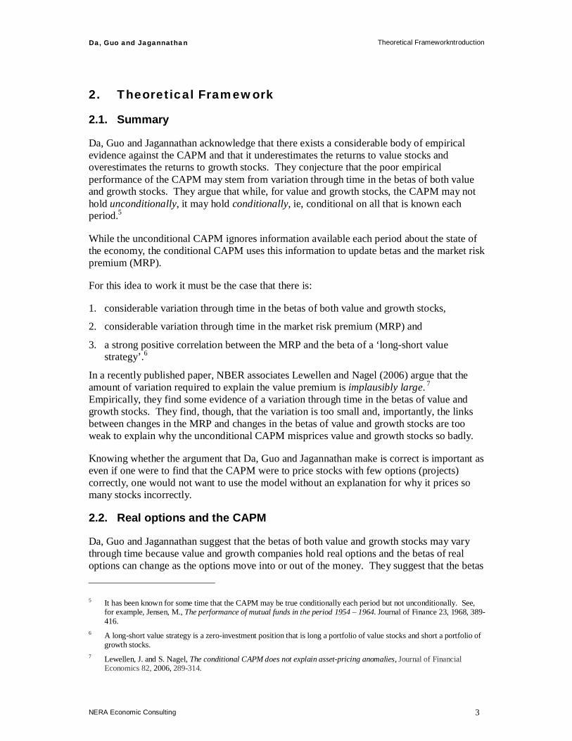
Da, Guo and Jagannathan acknowledge that there exists a considerable body of empirical evidence against the CAPM and that it underestimates the returns to value stocks and overestimates the returns to growth stocks. They conjecture that the poor empirical performance of the CAPM may stem from variation through time in the betas of both value and growth stocks. They argue that while, for value and growth stocks, the CAPM may not hold unconditionally, it may hold conditionally, ie, conditional on all that is known each period.5
While the unconditional CAPM ignores information available each period about the state of the economy, the conditional CAPM uses this information to update betas and the market risk premium (MRP).
For this idea to work it must be the case that there is:
1. considerable variation through time in the betas of both value and growth stocks,
2. considerable variation through time in the market risk premium (MRP) and
3. a strong positive correlation between the MRP and the beta of a ‘long-short value strategy’.6
In a recently published paper, NBER associates Lewellen and Nagel (2006) argue that the amount of variation required to explain the value premium is implausibly large. 7 Empirically, they find some evidence of a variation through time in the betas of value and growth stocks. They find, though, that the variation is too small and, importantly, the links between changes in the MRP and changes in the betas of value and growth stocks are too weak to explain why the unconditional CAPM misprices value and growth stocks so badly.
Knowing whether the argument that Da, Guo and Jagannathan make is correct is important as even if one were to find that the CAPM were to price stocks with few options (projects) correctly, one would not want to use the model without an explanation for why it prices so many stocks incorrectly.
2.2. Real options and the CAPM
Da, Guo and Jagannathan suggest that the betas of both value and growth stocks may vary through time because value and growth companies hold real options and the betas of real options can change as the options move into or out of the money. They suggest that the betas 5 It has been known for some time that the CAPM may be true conditionally each period but not unconditionally. See,
for example, Jensen, M., The performance of mutual funds in the period 1954 – 1964. Journal of Finance 23, 1968, 389-416.
6 A long-short value strategy is a zero-investment position that is long a portfolio of value stocks and short a portfolio of growth stocks.
7 Lewellen, J. and S. Nagel, The conditional CAPM does not explain asset-pricing anomalies, Journal of Financial Economics 82, 2006, 289-314.
Da, Guo and Jagannathan Theoretical Frameworkntroduction
NERA Economic Consulting 4
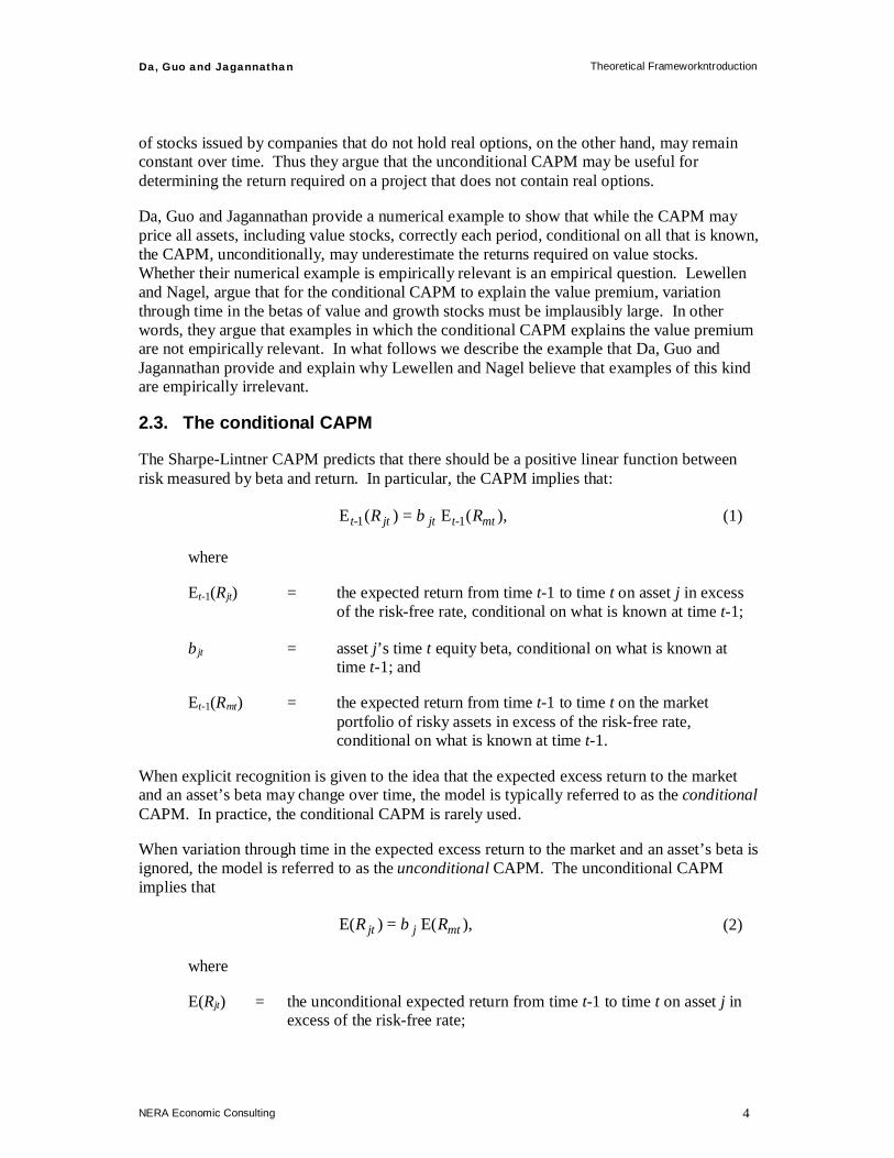
of stocks issued by companies that do not hold real options, on the other hand, may remain constant over time. Thus they argue that the unconditional CAPM may be useful for determining the return required on a project that does not contain real options.
Da, Guo and Jagannathan provide a numerical example to show that while the CAPM may price all assets, including value stocks, correctly each period, conditional on all that is known, the CAPM, unconditionally, may underestimate the returns required on value stocks. Whether their numerical example is empirically relevant is an empirical question. Lewellen and Nagel, argue that for the conditional CAPM to explain the value premium, variation through time in the betas of value and growth stocks must be implausibly large. In other words, they argue that examples in which the conditional CAPM explains the value premium are not empirically relevant. In what follows we describe the example that Da, Guo and Jagannathan provide and explain why Lewellen and Nagel believe that examples of this kind are empirically irrelevant.
2.3. The conditional CAPM
The Sharpe-Lintner CAPM predicts that there should be a positive linear function between risk measured by beta and return. In particular, the CAPM implies that:
),(E)(E 11 mtt-jtjtt- RR β= (1)
where
Et-1(Rjt) = the expected return from time t-1 to time t on asset j in excess of the risk-free rate, conditional on what is known at time t-1;
βjt = asset j’s time t equity beta, conditional on what is known at time t-1; and
Et-1(Rmt) = the expected return from time t-1 to time t on the market portfolio of risky assets in excess of the risk-free rate, conditional on what is known at time t-1.
When explicit recognition is given to the idea that the expected excess return to the market and an asset’s beta may change over time, the model is typically referred to as the conditional CAPM. In practice, the conditional CAPM is rarely used.
When variation through time in the expected excess return to the market and an asset’s beta is ignored, the model is referred to as the unconditional CAPM. The unconditional CAPM implies that
),E()E( mtjjt RR β= (2)
where
E(Rjt) = the unconditional expected return from time t-1 to time t on asset j in excess of the risk-free rate;

Da, Guo and Jagannathan Theoretical Frameworkntroduction
NERA Economic Consulting 5
βj = asset j’s unconditional beta; and
E(Rmt) = the unconditional expected return from time t-1 to time t on the market portfolio of risky assets in excess of the risk-free rate.
In practice, the unconditional CAPM is the version of the model that is typically used. For example, Australian regulators use a version of the CAPM in which the expected excess return to the market and the unconditional beta of the equity of a benchmark business remain constant within a period covered by an access arrangement.
A casual analysis might suggest that if the conditional CAPM were to hold period by period, then the unconditional CAPM would also have to be true. However, this is not the case. Set aside for the moment differences between unconditional betas and the means of their conditional counterparts. A comparison of (1) with (2) indicates that, if the conditional CAPM (1) is true, the unconditional CAPM (2) will be true only if βjt and Et-1(Rmt) do not covary with one another. This is because the expectation of the product of two random variables will only equal the product of the expectations of the two variables if the two variables are uncorrelated with one another. If instead βjt and Et-1(Rmt) covary positively (negatively) with one another, the unconditional CAPM (2) will underestimate (overestimate) the unconditional return required on asset j. So the error with which the unconditional CAPM measures the return required on an asset, that is, the asset’s unconditional alpha, will be, approximately:8
))(ECov( 1 mtt-jtUj R,βα = (3)
It is known that the unconditional CAPM underestimates the returns required on value stocks. For the conditional CAPM to price these stocks correctly period by period, it must be the case that the betas of value stocks covary positively with the MRP. Da, Guo and Jagannathan provide a numerical example to show how this might occur. We describe this example next.
Da, Guo and Jagannathan provide a two-period binomial example in which the conditional CAPM holds each period but in which the beta of a value stock increases when the MRP rises and falls as the MRP falls. The beta of the value stock changes through time because value firms are assumed to have real options whose betas change through time. The fact that the distribution of returns is binomial means that at the end of the first period there are only two outcomes one need consider. In the example, the risk-free rate is 2.47 percent per period but the required return on the market portfolio, which is 5 percent in the first period, can either fall to 3.5 percent or rise to 6.5 percent in the second period.
Figure 2.1 illustrates how the example works. The upper left panel shows that in the first period the conditional CAPM correctly prices the value option. The option has a beta above one and so the return required on the option exceeds the 5 percent return required on the 8 Jagannathan, R., and Z. Wang, The conditional CAPM and the cross-section of expected returns, Journal of Finance 51,
1996, 3–53. Lewellen, J. and S. Nagel, The conditional CAPM does not explain asset-pricing anomalies, Journal of Financial Economics 82, 2006, 289-314.
Da, Guo and Jagannathan Theoretical Frameworkntroduction
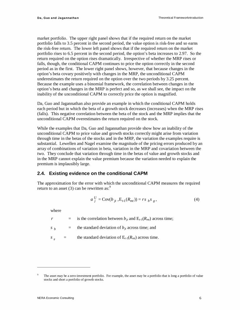
NERA Economic Consulting 6
market portfolio. The upper right panel shows that if the required return on the market portfolio falls to 3.5 percent in the second period, the value option is risk-free and so earns the risk-free return. The lower left panel shows that if the required return on the market portfolio rises to 6.5 percent in the second period, the option’s beta increases to 2.97. So the return required on the option rises dramatically. Irrespective of whether the MRP rises or falls, though, the conditional CAPM continues to price the option correctly in the second period as in the first. The lower right panel shows, however, that because changes in the option’s beta covary positively with changes in the MRP, the unconditional CAPM underestimates the return required on the option over the two periods by 3.25 percent. Because the example uses a binomial framework, the correlation between changes in the option’s beta and changes in the MRP is perfect and so, as we shall see, the impact on the inability of the unconditional CAPM to correctly price the option is magnified.
Da, Guo and Jagannathan also provide an example in which the conditional CAPM holds each period but in which the beta of a growth stock decreases (increases) when the MRP rises (falls). This negative correlation between the beta of the stock and the MRP implies that the unconditional CAPM overestimates the return required on the stock.
While the examples that Da, Guo and Jagannathan provide show how an inability of the unconditional CAPM to price value and growth stocks correctly might arise from variation through time in the betas of the stocks and in the MRP, the variation the examples require is substantial. Lewellen and Nagel examine the magnitude of the pricing errors produced by an array of combinations of variation in beta, variation in the MRP and covariation between the two. They conclude that variation through time in the betas of value and growth stocks and in the MRP cannot explain the value premium because the variation needed to explain the premium is implausibly large.
2.4. Existing evidence on the conditional CAPM
The approximation for the error with which the unconditional CAPM measures the required return to an asset (3) can be rewritten as:9
,R, mtt-jtUj γβσρσβα == ))(ECov( 1 (4)
where
ρ = is the correlation between βjt and Et-1(Rmt) across time;
βσ = the standard deviation of βjt across time; and
γσ = the standard deviation of Et-1(Rmt) across time.
9 The asset may be a zero-investment portfolio. For example, the asset may be a portfolio that is long a portfolio of value
stocks and short a portfolio of growth stocks.

Da, Guo and Jagannathan Theoretical Framework
NERA Economic Consulting 7
Figure 2.1 Return and beta in the Da, Guo and Jagannathan example.10
10 Note: F is the risk-free asset, M, the market portfolio and V the value option
0.00
0.02
0.04
0.06
0.08
0.10
0.12
0.14
0.16
0.0 0.5 1.0 1.5 2.0 2.5 3.0 3.5
MEA
N R
ETU
RN
BETA
CONDITIONAL: FIRST PERIOD
M
V
F
0.00
0.02
0.04
0.06
0.08
0.10
0.12
0.14
0.16
0.0 0.5 1.0 1.5 2.0 2.5 3.0 3.5
MEA
N R
ETU
RN
BETA
CONDITIONAL: SECOND PERIOD, HIGH EQUITY PREMIUM
M
V
F
0.00
0.02
0.04
0.06
0.08
0.10
0.12
0.14
0.16
0.0 0.5 1.0 1.5 2.0 2.5 3.0 3.5
MEA
N R
ETU
RN
BETA
CONDITIONAL: SECOND PERIOD, LOW EQUITY PREMIUM
MF, V
0.00
0.02
0.04
0.06
0.08
0.10
0.12
0.14
0.16
0.0 0.5 1.0 1.5 2.0 2.5 3.0 3.5
MEA
N R
ETU
RN
BETA
UNCONDITIONAL : BOTH PERIODS
M
V
F

Da, Guo and Jagannathan Theoretical Framework
NERA Economic Consulting 8
Thus the error with which the unconditional CAPM measures the required return to an asset will be higher, all else constant, the higher the correlation between the beta of the asset βjt and the market risk premium Et-1(Rmt) across time, the higher the standard deviation of βjt across time and the higher the standard deviation of Et-1(Rmt) across time. Lewellen and Nagel compute the approximate error with which the unconditional CAPM will price an asset for an array of values for these parameters and we reproduce their results below.
They consider two values for the correlation between the beta of the asset βjt and the market risk premium Et-1(Rmt):
60.=ρ and ..01=ρ
All else constant, a value for the correlation coefficient of one provides an upper bound on the error with the unconditional CAPM measures the required return to an asset. They consider three values for the standard deviation of βjt across time:
5030 .,. == ββ σσ and ..70=βσ
If the mean of the distribution of βjt across time were to be zero, then a value for the standard deviation of 0.5 would imply that approximately 95 percent of the time βjt lies between minus one and one. Thus a standard deviation of 0.5 allows for a substantial variation in beta.
Finally, they consider five values for the standard deviation of Et-1(Rmt) across time:
40302010 .,.,.,. ==== γγγγ σσσσ and ..50=γσ
If the mean of the distribution of Et-1(Rmt) across time were to be 0.5 percent per month, then a value for the standard deviation of 0.5 would imply that approximately 95 percent of the time Et-1(Rmt) lies between –0.5 percent per month and 1.5 percent per month or between approximately –6 percent per annum and 18 percent per annum. Thus a standard deviation of 0.5 allows for very large changes in the MRP across time.
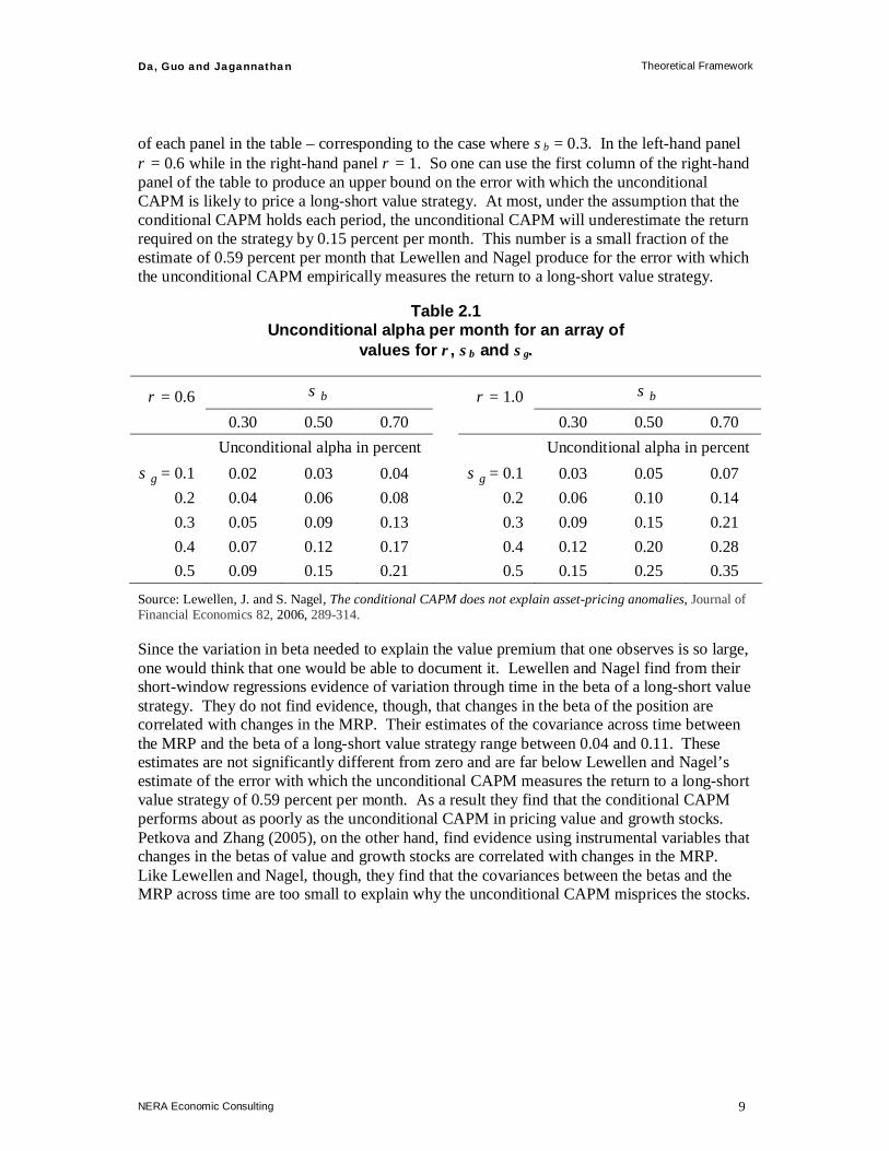
Table 2.1 shows the error with which the unconditional CAPM measures the monthly return required on an asset under the assumption that the conditional CAPM holds each period for various combinations of the parameters. To put the numbers into perspective, Lewellen and Nagel estimate that the error with which the unconditional CAPM measures the return to a long-short value strategy is 0.59 percent per month. Again, a long-short value strategy is a zero-investment position that is long a portfolio of value stocks and short a portfolio of growth stocks. Table 2.1 shows that even with the most extreme combination of parameters, the error with which the unconditional CAPM measures the return required on an asset does not exceed 0.35 percent per month.
Lewellen and Nagel use daily data and short-window regressions to estimate time series of conditional betas for value and growth portfolios. These time series suggest that a reasonable estimate of the standard deviation of the beta of a long-short value strategy is 0.25. Table 2.1 considers three values for σβ: 0.3, 0.5 and 0.7. Evidence that σβ does not exceed 0.25 indicates that, for a long-short value strategy, one can limit one’s attention to the first column
Da, Guo and Jagannathan Theoretical Framework
NERA Economic Consulting 9
of each panel in the table – corresponding to the case where σβ = 0.3. In the left-hand panel ρ = 0.6 while in the right-hand panel ρ = 1. So one can use the first column of the right-hand panel of the table to produce an upper bound on the error with which the unconditional CAPM is likely to price a long-short value strategy. At most, under the assumption that the conditional CAPM holds each period, the unconditional CAPM will underestimate the return required on the strategy by 0.15 percent per month. This number is a small fraction of the estimate of 0.59 percent per month that Lewellen and Nagel produce for the error with which the unconditional CAPM empirically measures the return to a long-short value strategy.
Table 2.1 Unconditional alpha per month for an array of
values for ρ, σβ and σγ.
ρ = 0.6 βσ ρ = 1.0 βσ
0.30 0.50 0.70 0.30 0.50 0.70 Unconditional alpha in percent Unconditional alpha in percent
γσ = 0.1 0.02 0.03 0.04 γσ = 0.1 0.03 0.05 0.07 0.2 0.04 0.06 0.08 0.2 0.06 0.10 0.14 0.3 0.05 0.09 0.13 0.3 0.09 0.15 0.21 0.4 0.07 0.12 0.17 0.4 0.12 0.20 0.28 0.5 0.09 0.15 0.21 0.5 0.15 0.25 0.35
Source: Lewellen, J. and S. Nagel, The conditional CAPM does not explain asset-pricing anomalies, Journal of Financial Economics 82, 2006, 289-314.
Since the variation in beta needed to explain the value premium that one observes is so large, one would think that one would be able to document it. Lewellen and Nagel find from their short-window regressions evidence of variation through time in the beta of a long-short value strategy. They do not find evidence, though, that changes in the beta of the position are correlated with changes in the MRP. Their estimates of the covariance across time between the MRP and the beta of a long-short value strategy range between 0.04 and 0.11. These estimates are not significantly different from zero and are far below Lewellen and Nagel’s estimate of the error with which the unconditional CAPM measures the return to a long-short value strategy of 0.59 percent per month. As a result they find that the conditional CAPM performs about as poorly as the unconditional CAPM in pricing value and growth stocks. Petkova and Zhang (2005), on the other hand, find evidence using instrumental variables that changes in the betas of value and growth stocks are correlated with changes in the MRP. Like Lewellen and Nagel, though, they find that the covariances between the betas and the MRP across time are too small to explain why the unconditional CAPM misprices the stocks.

Da, Guo and Jagannathan Data and Methodology
NERA Economic Consulting 10
3. Data and Methodology
3.1. Summary
Da, Guo and Jagannathan (2009) use NYSE-AMEX-NASDAQ data but exclude from their sample a substantial number of the stocks of small firms. Many of these stocks may also be value stocks since value stocks tend to be stocks with low market capitalisations. The Sharpe-Lintner CAPM is known to misprice low market capitalisation stocks and value stocks and so excluding these stocks may reduce the apparent evidence against the model. Excluding these stocks may also lower the apparent benefit to using the Fama-French three-factor model since the model does a better job of pricing the stocks of small firms and value stocks than does the Sharpe-Lintner CAPM.
In many of their tests, Da, Guo and Jagannathan follow Hoberg and Welch (2007) and use betas computed from data that excludes the recent past.11 They do so because they believe that investors may be slow to recognise changes in betas. They call these betas ‘aged’ betas. The theoretical justification for the idea of using aged betas is weak. So weak, in fact, that Hoberg and Welch have withdrawn their work from circulation. 12 Since one can use high-frequency data to improve the precision with which one estimates a stock’s beta, it is difficult to see why investors should be slow to recognise changes in the parameter. Even if one were to believe that investors are slow to recognise changes in a stock’s beta, there is no theory to indicate exactly how slow investors might be to recognise changes. Thus one must in some way use the data to infer the extent to which investors are slow to recognise changes. Doing so, however, complicates inference.
These issues would normally be raised by a referee or referees before publication and Da, Guo and Jagannathan would have opportunities to respond. In the absence of a pre-publication peer review, however, we do not see how one can rely on the results in Da, Guo and Jagannathan’s paper without additional analysis being undertaken to address the issues we raise.
3.2. Excluded data
Instead of testing directly whether variation in the MRP and the betas of value and growth stocks can explain the poor performance of the unconditional CAPM, Da, Guo and Jagannathan test whether the unconditional CAPM can correctly price the stocks of firms they believe hold few real options. They use data from the Center for Research in Security Prices (CRSP) from 1932 to 2007 to conduct these tests but they make several cuts to the data. In what follows we describe the cuts that they make and evaluate the likely impact of the cuts on tests of the CAPM and of the Fama-French three-factor model.
At the end of each June, Da, Guo and Jagannathan use a number of screens to eliminate stocks from their sample. First, they eliminate firms with a market capitalisation less than the NYSE 10th percentile breakpoint. Second, they eliminate firms whose price is less than five 11 Hoberg, G. And I. Welch, Aged and recent market betas in securities pricing, Working paper withdrawn from
circulation, Brown University, 2007. 12 See http://welch.econ.brown.edu/academics/.
Da, Guo and Jagannathan Data and Methodology
NERA Economic Consulting 11
dollars. Third, they eliminate firms whose returns over the prior 12 months place them in the top or bottom momentum deciles. Fourth, they eliminate firms listed for less than three years.
Da, Guo and Jagannathan state that after applying these filters, their sample still contains 75 per cent of the universe of CRSP stocks by market capitalisation. This statement, though, does not imply that they only remove 25 percent of the stocks that the CRSP database contains. Their cuts are likely to eliminate around 30 percent of firms prior to the addition of AMEX stocks to the CRSP database in 1962, a larger fraction of firms between 1962 and the introduction of NASDAQ firms to the database in 1972 and an even larger fraction of firms from there on. The cuts are likely to eliminate large numbers of AMEX and NASDAQ stocks from their sample because they employ the NYSE 10th percentile breakpoint to cut small firms and the typical AMEX firm and typical NASDAQ firm are smaller than the typical NYSE firm. Since value firms are often small firms, they may also eliminate many value firms. Cutting small firms and value firms from their sample may improve the apparent performance of the Sharpe-Lintner CAPM since there is ample evidence that the model misprices the stocks of small firms and value firms. Conversely, cutting small firms and value firms from their sample may reduce the apparent benefit to using the Fama-French three-factor model since the model does a better job of pricing the stocks of small firms and value stocks.
On the other hand, eliminating recent past losers and winners may improve the apparent performance of both the Sharpe-Lintner CAPM and the Fama-French model because both models misprice portfolios of recent past losers and winners.
The methodology for testing linear pricing models like the Sharpe-Lintner CAPM and the Fama-French model is well established and, for the most part, Da, Guo and Jagannathan use conventional methods. The method they use for computing betas to be employed in cross-sectional tests of the models, though, is unusual and may have an impact on the inferences they draw and so we discuss the method in some detail.
3.3. Aged betas
A line of research in finance suggests that investors are slow to learn about the behaviour of returns. Da, Guo and Jagannathan suggest that for this reason one should use estimates of beta computed from data that exclude the most recent two years’ worth of returns. They cite for support of this idea a paper by Hoberg and Welch. Unfortunately, Hoberg and Welch have withdrawn their work from circulation because they ‘no longer believe that the theory (of slow recognition by investors) is correct.’13 The withdrawal of their paper from circulation makes understanding what was their original rationale for computing ‘aged betas’ difficult. It also makes it difficult to know why they chose to exclude two years’ worth of data and not less data or more data.
There are good reasons why one would expect investors not to be slow to recognise changes in risk. It is well known that, while it is difficult to estimate precisely the mean return to a portfolio, it is less difficult to estimate precisely the risk of the portfolio. It is also well
13 See http://welch.econ.brown.edu/academics/.

Da, Guo and Jagannathan Data and Methodology
NERA Economic Consulting 12
known that, while the use of high-frequency data cannot help one to produce a sharper estimate of the mean return to a portfolio, the use of high-frequency data can help one produce a sharper estimate of the risk of the portfolio. So it should be easier for investors to recognise changes in risk than changes in the returns required on assets.
To see this, consider a portfolio whose annual return is distributed with a mean of 12 percent and a standard deviation of 24 percent. The sample mean of the return to the portfolio on an annual basis computed from a sample of 10 years will be distributed with a mean of 12 percent and a standard deviation of 7.6 percent. This will be true, approximately, whether one uses 10 years’ worth of annual, monthly, weekly or daily data to compute the sample mean on an annual basis. In other words, the use of high-frequency data will not help one to produce a sharper estimate of the mean. The sample standard deviation on an annual basis computed from a sample of 10 years’ worth of annual (daily) data, on the other hand, will be approximately distributed with a mean of 24 percent and a standard deviation of 5.4 (0.3) percent. Thus one can increase the precision with which one estimates the standard deviation by using high-frequency data. Although here, for simplicity, risk is measured by standard deviation of return, the same argument will apply for risk measured by beta. Thus, while it may be difficult for an investor to recognise changes in mean returns, it should be considerably less difficult for an investor to recognise changes in risk measured either by beta or standard deviation of return.
Consistent with this analysis, the AER argues in the ActewAGL draft decision that investor perceptions of market volatility have undergone substantial changes over the last year.14 Changes over such a short period of time are difficult to reconcile with the idea that investors are slow to recognise changes in risk.
Even if one were to accept the idea, though, that investors are slow to recognise changes in risk, one faces the difficulty of determining exactly how slow investors are to recognise changes. Since theory provides little guide, one must in some way use the data to determine the pace at which investors recognise changes in risk. Using the data to determine the pace at which investors recognise changes, however, complicates inference. For example, if one has searched over windows for computing betas to meet some criterion, then inference must reflect the fact. The criterion might be to maximize the R-squared from a cross-sectional regression of return on beta. If one conducts a comprehensive search, one may be able to provide what appears to be convincing evidence of a strong relation between return and beta. The significance of the results that one reports, though, should reflect the extent of the search one has conducted. There is no indication that the inference that Da, Guo and Jagannathan draw reflects the search that Hoberg and Welch may have conducted over windows for estimating betas.
14 See ActewAGL draft decision, page 65.

Da, Guo and Jagannathan Empirical Evidence
NERA Economic Consulting 13
4. Empirical Evidence
4.1. Summary
Da, Gou and Jagannathan (2009) report evidence that indicates that across all of the stocks in their sample the Sharpe-Lintner CAPM does not hold. In particular, they provide evidence that the return to a zero-beta asset exceeds on average the risk-free rate and that the market price of risk is below the mean excess return to the market portfolio. In other words, consistent with many others, they find evidence that the Sharpe-Lintner CAPM underestimates the returns to low-beta assets. Since the AER views the equity of a benchmark gas distribution business as a low-beta asset, this evidence suggests that the use of the Sharpe-Lintner CAPM by the AER will produce an underestimate of the return the market requires on the equity.
It could be argued that a high R-squared from a cross-sectional regression of return on beta provides support for the Sharpe-Lintner CAPM. This would be untrue. A high R-squared from a cross-sectional regression of return on beta does not mean that the Sharpe-Lintner CAPM is correct. This is because the statistic does not measure whether the restrictions the model imposes on the intercept and slope coefficient from the regression are satisfied.
Da, Guo and Jagannathan conjecture that the book-to-market effect is a within-industries effect and not an across-industries effect. So they argue that although the Sharpe-Lintner CAPM may not hold at the individual stock level, the model may hold at the industry or sector level. The evidence that Da, Guo and Jagannathan provide, however, does not support their conjecture.
Da, Gou and Jagannathan report evidence that indicates that the Sharpe-Lintner CAPM does not hold for stocks that they believe have few real options – stocks of firms with low capex. They find that in a cross-sectional regression of return on beta, size and book-to-market that size and book-to-market matter. In other words, contrary to the predictions of the CAPM, they find that variables other than beta can explain the cross-section of returns. This evidence suggests that additional factors beyond an asset’s beta are required to measure the return the market requires on the asset. The Fama-French model provides such additional factors.
4.2. Roll’s critique
Da, Guo and Jagannathan conduct two types of tests: time-series tests and cross-sectional tests. Before we do so, however, we address Roll’s critique since Handley has raised the issue several times. 15
The Sharpe-Lintner CAPM predicts that the market portfolio will be mean-variance efficient. Theory suggests that the market portfolio should consist of all assets, not just stocks. Thus theory suggests that the market portfolio should include bonds, real estate and human capital. Measuring the returns to assets other than stocks, though, can be difficult. Corporate bonds are often infrequently traded, the quality of real estate traded changes through time in ways
15 Handley, John, A Note on the Valuation of Imputation Credits: Report for the Australian Energy Regulator, 12
November 2008.

Da, Guo and Jagannathan Empirical Evidence
NERA Economic Consulting 14
that are difficult to gauge and human capital is rarely traded. For these reasons, most academic work and most practitioners use the return to an index of stocks as a proxy for the return to the market portfolio.
While the use of a stock index as a proxy for the market portfolio is almost uniform, Roll (1977) emphasizes that the CAPM does not imply that a stock index should be mean-variance efficient.16 The CAPM implies only that the market portfolio should be efficient. So a test of the mean-variance efficiency of an index of stocks cannot be viewed as a test of the CAPM. A different issue concerns us, though, than that which concerns Roll. The issue that concerns us is whether an empirical version of the CAPM produces accurate estimates of required returns. The issue that concerns Roll, but not us here, is whether the CAPM itself is true. A test of the mean-variance efficiency of a stock index can be viewed as a test of whether the empirical version of the model that the AER uses produces accurate estimates of returns. This is the issue that concerns us. A test of the mean-variance efficiency of a stock index cannot be viewed as a test of the model itself. In other words, we think that Roll is right. Discovering whether the model is really true, though, is not an issue that concerns us here.
For simplicity, from henceforth, when we refer to a test of the CAPM, we refer to a test of the empirical version of the model that practitioners use and not necessarily the model itself.
4.3. Time-series tests
Time-series tests of the Sharpe-Lintner CAPM use regressions of the form
,jtmtjjjt RR εβα ++= (5)
where
Rjt = is the return from time t-1 to time t on asset j in excess of the risk-free rate;
αj = asset j’s alpha – the error with which the CAPM measures the return required on asset j;
βj = asset j’s equity beta;
Rmt = the return from time t-1 to time t on the market portfolio of risky assets in excess of the risk-free rate; and
εjt = a regression disturbance.
If the CAPM is true
.allfor0:H0 jj =α
Time series tests of the Fama-French model work in a similar way.
16 Roll, Richard, A critique of the asset pricing theory’s tests: Part I, Journal of Financial Economics 4, 1977, pages 129-
176.

Da, Guo and Jagannathan Empirical Evidence
NERA Economic Consulting 15
Da, Guo and Jagannathan use 10 portfolios formed on the basis of prior beta estimates to test the Sharpe-Lintner CAPM and Fama-French model. The time-series tests of the model that they conduct that use these portfolios reject both models. They find, consistent with the evidence that Lewellen, Nagel and NBER associate Shanken (2008) provide, that both models underestimate the returns to low-beta stocks.17 Time-series tests that they conduct that use portfolios formed on the basis of aged betas, on the other hand, reject neither model. It is likely, though, that had they tested the two models against, not a vague alternative, but zero-beta versions of the models, they would have rejected the Sharpe-Lintner CAPM and Fama-French model. This is because, even with portfolios formed on the basis of aged betas, their evidence suggests that both the Sharpe-Lintner CAPM and Fama-French model underestimate the returns to low-beta stocks.
As Da, Guo and Jagannathan point out, portfolios formed on the basis of prior beta estimates display little variation in their exposures to the Fama-French HML and SMB factors.18 So tests that use the portfolios are unlikely to uncover evidence that the Fama-French model offers an improvement over the Sharpe-Lintner CAPM. The advantage of the Fama-French model over the Sharpe-Lintner CAPM is that it can better measure the returns required on portfolios formed on the basis of size and book-to-market.
4.4. Cross-sectional tests
Da, Guo and Jagannathan also conduct cross-sectional tests of the Sharpe-Lintner CAPM and the Fama-French model. The cross-sectional tests that they conduct of the Sharpe-Lintner CAPM use Fama-MacBeth regressions of the form
,210 jtjttjtttjt ZR ηδβδδ +++= (6)
where
δ0t = the regression intercept;
δ1t = a regression parameter;
δ2t = a vector of regression parameters;
Zjt = a vector of regressors known at time t-1; and
ηjt = a regression disturbance.
If the Sharpe-Lintner CAPM is true, then on average δ0t and δ2t should be zero. δ0t should be zero because the Sharpe-Lintner CAPM says that the mean excess return on a zero-beta asset
17 Lewellen, J., S. Nagel and J. Shanken, A skeptical appraisal of asset pricing tests, Journal of Financial Economics, forthcoming.
18 HML is the return to a zero-investment position that is long a portfolio of value stocks and short a portfolio of growth
stocks. SMB is the return to a zero-investment position that is long a portfolio of low market capitalisation stocks and short a portfolio of high market capitalisation stocks.

Da, Guo and Jagannathan Empirical Evidence
NERA Economic Consulting 16
should be zero. δ2t should be zero because the Sharpe-Lintner CAPM says that only beta should explain the cross-section of excess returns. Conditional on beta, no other variables should be useful in explaining the cross-section of returns. δ1t should on average equal the MRP.
Cross-sectional tests of the Fama-French model work in a similar way.
Da, Guo and Jagannathan also report the R-squared of each cross-sectional regression. As Lewellen, Nagel and Shanken emphasise, however, the R-squared from a cross-sectional regression of return on risk is an unreliable measure of the ability of a pricing model to correctly price assets. One reason it is an unreliable measure is that the statistic does not depend on whether the restrictions placed on the means of the regression parameters δ0t, δ1t and δ2t hold. So it is possible for the R-squared from a cross-sectional regression of return on beta to be high when the Sharpe-Lintner CAPM is false. Indeed we will emphasize that some of the results that Da, Guo and Jagannathan report indicate that there is a strong relation between return and beta but that simultaneously one can reject the Sharpe-Lintner CAPM. It is also possible for the R-squared from a cross-sectional regression of return on beta to be low when the Sharpe-Lintner CAPM is true.
The cross-sectional tests that Da, Guo and Jagannathan conduct, are reproduced below in Table 4.1 the results of Panel D of their Table 2.
Table 4.1 Regressions of excess returns on beta19
Beta
Zero-beta excess return
Price of risk
R-squared
Conventional 0.63 0.19 38.80 (4.14) (0.67) Aged 0.40 0.33 80.99 (2.39) (1.27) Source: Da, Guo and Jagannathan, CAPM for Estimating the Cost of Equity Capital: Interpreting the Empirical Evidence, 2009, NBER Working Paper, Table 2, Panel D.
The cross-sectional results indicate that the Sharpe-Lintner CAPM can be rejected using either conventional or aged betas. The model can be rejected because the zero-beta excess return is significantly positive whether conventional or aged betas are used.
To understand the implications of these results for estimating required returns, consider an asset that has, like the equity of a benchmark gas distribution business, a beta of 0.8. The mean excess return to a value-weighted portfolio of NYSE-AMEX-NASDAQ stocks in excess of the one-month bill rate from 1932 to 2007 is 0.73 percent per month according to Ken French’s web site. This figure matches precisely an estimate computed using the aged 19 The zero-beta excess return and the price of risk are in percent per month. t test statistics are in parentheses.

Da, Guo and Jagannathan Empirical Evidence
NERA Economic Consulting 17
regression in Table 4.1. With this value for the market price of risk, the return required on an asset with a beta of 0.8 must be, if the Sharpe-Lintner CAPM is true, 0.8 × 0.73 = 0.58 percent per month. The aged results from Table 4.1, on the other hand, indicate that the return required on the asset should be 0.40 + 0.8 × 0.33 = 0.66 percent per month. In other words, the aged results indicate that the return required should be about 100 basis points higher per annum than the Sharpe-Lintner CAPM predicts. In other words, the results indicate that the Sharpe-Lintner CAPM underestimates the returns to low-beta assets.
It would be tempting to incorrectly attribute the high R-squared in Table 4.1 for the aged equity beta as a sign that the Sharpe CAPM is a good predictive tool. The R-squared from a cross-sectional regression of return on beta does not measure the ability of the Sharpe-Lintner CAPM to correctly price assets. Again, the statistic does not depend on whether the restrictions the model places on the parameters of the regression are true or false. A strong relation between return and beta, that is, a high R-squared, does not imply that the Sharpe-Lintner CAPM is correct. Similarly a weak relation between return and beta, that is, a low R-squared, does not imply that the Sharpe-Lintner CAPM is false.
The cross-sectional results that Da, Guo and Jagannathan report also indicate, consistent with the evidence that Lewellen, Nagel and Shanken provide, that the Fama-French model underestimates the returns required on low-beta assets. Thus the use of the Fama-French model to estimate the return required on an asset with a beta of 0.8 will tend to produce an estimate that is too low.
As Da, Guo and Jagannathan point out, portfolios formed on the basis of prior beta estimates display little variation in their exposures to the Fama-French HML and SMB factors. So, again, tests that use the portfolios are unlikely to uncover evidence that the Fama-French model offers an improvement over the Sharpe-Lintner CAPM. Consistent with this analysis, Da, Guo and Jagannathan find little evidence of a relation between the returns to the beta-sorted portfolios and their exposures to the Fama-French factors.
The results of the tests, though, should not be interpreted as evidence that the additional explanatory power of the Fama–French factors is small. The tests are designed in such a way as to hide the ability of the Fama-French model to correctly price the stocks of small firms and value stocks. They are also designed in such a way as to hide the inability of the Sharpe-Lintner CAPM to correctly price these stocks. Tests that use portfolios sorted on the basis of size and book-to-market produce very different results.20
The results in Table 4.1 mask a well known difference between the relation between return and beta in the earlier part of the period that Da, Guo and Jagannathan examine and the relation in the later part. In the earlier part of their sample the existing evidence indicates that there is a positive relation between return and beta. The evidence indicates, though, that there is little relation between the two variables in the later part of the sample. Table 4.2 summarizes the existing evidence and illustrates that in the period since 1963 the zero beta excess return is positive and statistically significant and there is an insignificant negative
20 Fama, Eugene and Kenneth French, The capital asset pricing model: Theory and evidence, Journal of Economic
Perspectives 18, 2004, pages 25-46.

Da, Guo and Jagannathan Empirical Evidence
NERA Economic Consulting 18
relation between risk and return. In other words, the post-1963 evidence indicates that the CAPM substantially underestimates the returns required on low-beta stocks.
While we do not suggest that the positive relation between return and beta documented in the earlier part of the sample is unimportant, the absence of a relation between return and beta over the last 40 or 50 years makes it difficult to be enthusiastic about using the CAPM.
Table 4.2 Summary of existing evidence on the CAPM21
Study
Period
Zero-beta excess return
Price of risk
Fama and MacBeth (1973) 1935-1968 0.48 0.85 (0.19) (0.33) Campbell (2004) 1929-1963 0.23 0.51 (0.28) (0.46) Lewellen, Nagel and Shanken (2008) 1963-2004 0.73 -0.11 (0.23) (0.28) Campbell (2004) 1963-2001 0.69 -0.07 (0.26) (0.34) Sources: Fama, E and J. MacBeth, Risk, return, and equilibrium: Empirical tests, Journal of Political Economy 71, pages 607-636.
Campbell, J. And T. Vuolteenaho, Bad beta, good beta, American Economic Review 94, pages 1249-1275.
Lewellen, J., S. Nagel and J. Shanken, A skeptical appraisal of asset pricing tests, Journal of Financial Economics, forthcoming.
4.5. Industry returns
Tests of the Sharpe-Lintner CAPM and Fama-French model that Fama and French (1993) conduct use portfolios formed on the basis of size and book-to-market.22 Fama and French use portfolios formed on the basis of size and book-to-market because it is known that the Sharpe-Lintner CAPM is unable to correctly price the portfolios. Forming portfolios in this way also creates a large variation across the portfolios in their exposures to the Fama-French SMB and HML factors. Besides forming portfolios on the basis of prior estimates of beta, Da, Guo and Jagannathan also form portfolios on the basis of industry membership and book-to-market.
21 The zero-beta excess return and price of risk are in percent per month. Standard errors are in parentheses. 22 Fama, Eugene and Kenneth French, Common risk factors in the returns to stocks and bonds, Journal of Financial
Economics 33, 1993, pages 3-56.

Da, Guo and Jagannathan Empirical Evidence
NERA Economic Consulting 19
Da, Guo and Jagannathan conjecture that the book-to-market effect is a within-industries effect and not an across-industries effect. They argue that although the Sharpe-Lintner CAPM may not hold at the individual stock level, the model may hold at the industry level. If the Sharpe-Lintner CAPM were to hold at the industry level, then the model would be the ideal tool for determining the return required on the equity of a benchmark business. The evidence that Da, Guo and Jagannathan provide, however, does not support their conjecture – although, as we shall explain, this is not the way in which they interpret their evidence.
The conjecture that Da, Guo and Jagannathan make is essentially that deviations from the Sharpe-Lintner CAPM at the stock level may be difficult to detect in industry portfolios because in any industry portfolio there may be as many stocks whose returns are underestimated by the CAPM as stocks whose returns are overestimated. If their conjecture is correct, then tests of the CAPM that use industry portfolios may lack power. In other words, tests that use industry portfolios may have difficulty rejecting the CAPM when it is false. So it may not be a good idea to rely on tests that use industry portfolios. This is because while it may be true for many industries that there are as many stocks whose returns are underestimated by the CAPM as stocks whose returns are overestimated, it may not be true of all industries.
It may also be the case that for many industries there are as many stocks with positive HML exposures as there are stocks with negative HML exposures. Thus there may be less variation across industry portfolios in HML exposures than across individual stocks. If this is true, then tests of the Sharpe-Lintner CAPM against the alternative that the Fama-French model is true that use industry portfolios may lack power. In other words, tests that use industry portfolios may have difficulty rejecting the CAPM in favour of the Fama-French model when the CAPM is false and the Fama-French model is true. So, again, it may not be a good idea to rely on tests that use industry portfolios. This is because while it may be true for many industries that there are as many stocks with positive HML exposures as there are stocks with negative HML exposures, it may not be true of all industries.
Evidence consistent with these arguments is provided by NERA (2009). 23 In that paper we examine the returns to portfolio of a US regulated energy utilities and find that while there is evidence that the Sharpe-Lintner CAPM significantly underestimates the return required on the portfolio, there is no evidence that the Fama-French model does so. We find that regulated energy utilities, like their Australian counterparts, have a positive exposure to the Fama-French HML factor. While the Sharpe-Lintner CAPM provides no compensation for this exposure, the Fama-French model does. For this reason, the Fama-French model provides a better fit for the data than does the Sharpe-Lintner CAPM.
To test their conjecture that the book-to-market effect is a within-industries effect and not an across-industries effect, Da, Guo and Jagannathan form 10 industry portfolios and then split each of these 10 portfolios into three book-to-market terciles. From each industry they choose one book-to-market tercile in such a way as to maximize the variation in book-to-market across the 10 portfolios chosen. They argue that if the book-to-market effect is a
23 NERA, Cost of equity - Fama-French three-factor model, Report prepared for Jemena, 7 August 2009.

Da, Guo and Jagannathan Empirical Evidence
NERA Economic Consulting 20
within-industries effect and not an across-industries effect, then the Sharpe-Lintner CAPM should price the 10 portfolios correctly and there should be no benefit to using the Fama-French model. Again, they conduct time series and cross-sectional tests.
Their results indicate that while they form portfolios in such a way as to maximize the variation across portfolios in book-to-market, there is a substantially smaller variation across the portfolios in their exposures to the Fama-French SMB and HML factors than is true across the 25 portfolios that Fama and French form on the basis of size and book-to-market. For example, none of the Da, Guo and Jagannathan portfolios have an absolute exposure to the SMB factor above 0.5 while 14 (56 percent) of the Fama-French portfolios have an absolute exposure above 0.5. Only 2 (20 percent) of the Da, Guo and Jagannathan portfolios have an absolute exposure to the HML factor above 0.5 while 9 (36 percent) of the Fama-French portfolios have an absolute exposure above 0.5.
Da, Guo and Jagannathan time-series tests indicate that both the Sharpe-Lintner and Fama-French models misprice the 10 industry portfolios. Of the three portfolios that have the highest exposure to the HML factor, the Sharpe-Lintner CAPM significantly underestimates the returns required on two while the Fama-French model prices the portfolios correctly. Of the three portfolios with the lowest exposure to the HML factor, the Fama-French model significantly overestimates the returns required on two while the Sharpe-Lintner CAPM prices the portfolios correctly.
Their cross-sectional tests indicate that one can reject the Sharpe-Lintner CAPM. We reproduce their Panel D, Table 3 as Table 4.3 below. While Da, Guo and Jagannathan report t test statistics, we report standard errors that we compute from the estimates and test statistics that they report, for reasons that we will make clear.
Table 4.3 Cross-sectional regressions for 10 maximum book-to-market dispersion
portfolios24
Exposure Intercept Market SMB HML
0.06 0.88
(0.26) (0.37)
0.73 0.08 0.10 0.62 (0.32) (0.40) (0.36) (0.27)
Source: Da, Guo and Jagannathan, CAPM for Estimating the Cost of Equity Capital: Interpreting the Empirical Evidence, 2009, NBER Working Paper, Table 3, Panel D.
Table 4.3 shows that in a cross-sectional regression of excess return on market, SMB and HML exposures, that uses the 10 industry portfolios, there is a significant relation only between a portfolio’s return and its HML exposure. The table also indicates that the return to 24 Estimates have been multiplied by 100. Standard errors are in parentheses.

Da, Guo and Jagannathan Empirical Evidence
NERA Economic Consulting 21
a zero-beta portfolio exceeds on average the risk-free rate. Both these pieces of evidence are inconsistent with the Sharpe-Lintner CAPM. The second piece of evidence is also inconsistent with the Fama-French model, but is consistent with the evidence that Lewellen, Nagel and Shanken provide. Again, Lewellen, Nagel and Shanken find that the Fama-French model underestimates the returns required on low-beta assets. So the use of the Fama-French model to estimate the return required on an asset with a beta of 0.8, for example, will tend to produce an estimate that is too low.
The interpretation that Da, Guo and Jagannathan place on their evidence on page 22 of their paper is that:
The loading on HML does seem to drive out the CAPM beta. However, the CAPM betas and the factor loadings on HML are highly correlated across the 10 portfolios. As a result, a problem of multicollinearity emerges. As a potential sign of such a problem, the intercept in the three-factor model is now significantly different from zero. In other words, the small improvement of the three-factor model over the standard CAPM in the cross-sectional analysis here has to be interpreted with caution.
Multicollinearity arises when there is an approximate linear relation between one regressor and another regressor or other regressors. The correlation between the market exposures and the HML exposures that Da, Guo and Jagannathan report for the 10 industry portfolios is 0.69. While there is no formal guide as to how close approximate the relation between two regressors must be before multicollinearity becomes a problem, a correlation this low would not normally be expected to give rise to a problem.
Peter Kennedy’s A guide to econometrics provides a clear discussion of the impact of multicollinearity.25 Multicollinearity does not give rise to bias but can lead to large standard errors. Table 4.3 indicates that the standard error on the market exposure rises from 0.37 to just 0.40 with the inclusion in the regression of the two Fama-French exposures. This strongly suggests that multicollinearity is not a problem. The large and significant intercept is not a sign of multicollinearity – because multicollinearity does not give rise to bias – but a sign that both the Fama-French model, like the Sharpe-Lintner CAPM, underestimates the returns required on low-beta assets.
4.6. Tests on low-capex stocks
The central hypothesis of Da, Guo and Jagannathan’s work is that value and growth stocks have real options whose betas change over time in such a way as to ensure that the unconditional CAPM misprices the stocks. To test this hypothesis they do not test directly whether changes in the betas of value and growth stocks over time can explain the inability of the unconditional CAPM to correctly price the stocks. Instead, they test whether the model can correctly price the stocks of firms that they believe do not hold real options – firms with low capital expenditure.
The results in Table 4.4 indicate that the unconditional CAPM can be rejected for both low-capex stocks and for high-capex stocks. The CAPM says that, conditional on beta, no other variables should be useful in explaining the cross-section of returns. The results in Table 4.4,
25 Kennedy, P., A guide to econometrics, Wiley-Blackwell, 2008.

Da, Guo and Jagannathan Empirical Evidence
NERA Economic Consulting 22
though, indicate that, conditional on an asset’s aged beta, size and book-to-market are useful in explaining the cross-section of returns.
However, the AER’s interpretation of the results is different. It states that:26
… even though the Sharpe–Lintner CAPM has limitations it still remains a well accepted model that explains the risk–return relationship. Recent academic research continues to support the Sharpe–Lintner CAPM as the best available predictor of returns from a capital asset, and it is particularly accurate under the circumstances applying to the benchmark efficient business.
This interpretation does not match the results that Da, Guo and Jagannathan report. Again, the results that Da, Guo and Jagannathan report indicate that the Sharpe-Lintner CAPM misprices firms that they believe have few real options.
The results that Da, Guo and Jagannathan provide indicate that besides an asset’s beta, size and book-to-market are useful in predicting the return on the stock of a company with few real options. Da, Guo and Jagannathan do not include as regressors in the cross-sectional tests that they conduct an asset’s exposure to the Fama-French SMB and HML factors. However, it is likely that, as Davis, Fama and French (2000) find, they would observe that if they replaced size and book to market with these exposures, the exposures like the characteristics would be useful in explaining the cross-section of returns as the Fama-French model predicts should be the case.27
Table 4.4 Cross-sectional regressions for low-capex and high-capex stocks28
Capex Aged beta Size Book-to-market Lowest 4.23 (1.82) 4.69 -1.23 4.33 (2.27) (-1.99) (3.08) Highest 0.75 (0.23) 1.26 -0.53 0.39 (0.44) (-0.87) (2.27)
26 See ActewAGL draft decision, page 63. 27 Davis, J., E. Fama, and K. French, Characteristics, covariances, and average returns: 1929-1997, Journal of Finance
55, 2000, 389–406. 28 Estimates have been multiplied by 100. t test statistics are in parentheses.

Da, Guo and Jagannathan Conclusions
NERA Economic Consulting 23
5. Conclusions
In a recent NBER working paper, Da, Guo and Jagannathan (2009) argue that the CAPM is a useful tool for valuing projects without real options. They acknowledge that the CAPM misprices value stocks. They argue, though, that the reason that it does so is because the stocks have real options whose betas vary substantially over time.
In this paper we review the arguments that Da, Guo and Jagannathan make and the empirical evidence that they produce. We point out that:
• Evidence provided by Lewellen and Nagel (2006) and Petkova and Zhang (2005) provide indicates that variation through time in the betas of value and growth stocks cannot explain why the CAPM misprices these stocks to the extent that it does. Their evidence indicates that there is not enough variation in the betas of the stocks to explain why the CAPM so badly underestimates the returns to value stocks.
If the CAPM holds it should correctly price all stocks, not just those with few real options. Without a convincing explanation of why the CAPM prices value stocks so badly, regulators should be cautious in relying on the advice that Da, Guo and Jagannathan provide – that it is safe to use the CAPM to estimate the returns required of stocks with few real options.
Da, Guo and Jagannathan eliminate a substantial number of smaller firms from their sample. We point out that:
• Many of these stocks may also be value stocks since value stocks tend to be those with low market capitalisations. The Sharpe-Lintner CAPM is known to misprice low market capitalisation and value stocks, and so excluding these stocks may reduce the apparent evidence against the CAPM. Excluding the stocks may also reduce the apparent benefit to using the Fama-French three-factor model since the model does a better job of pricing the stocks of small firms and value stocks than does the Sharpe-Lintner CAPM.
The elimination of a large number of stocks from the Da, Guo and Jagannathan study means that it cannot be used to draw a valid conclusion on the performance of the Fama-French three factor model.
In much of their empirical work Da, Guo and Jagannathan follow Hoberg and Welch (2007) and use betas computed from data that excludes the recent past. They do so because they believe that investors may be slow to recognise changes in betas. They call these betas ‘aged’ betas. We point out that:
• Hoberg and Welch have withdrawn their work from circulation because they ‘no longer believe that the theory (of slow recognition by investors) is correct.’29 Since one can use high-frequency data to improve the precision with which one estimates a stock’s beta, it is difficult to see why investors should be slow to recognise changes in the parameter.
29 See http://welch.econ.brown.edu/academics/.

Da, Guo and Jagannathan Conclusions
NERA Economic Consulting 24
There is limited academic support for the use of ‘aged betas’ and this is a further reason for regulators to be hesitant in relying on the conclusions of the Da, Guo and Jagannathan study.
Da, Guo and Jagannathan show an almost linear relation, across all stocks, between return and beta which may be construed as support for the Sharpe-Lintner CAPM. We point out that:
• An almost linear relation between return and beta does not imply that the Sharpe-Lintner CAPM is correct. The Sharpe-Lintner CAPM does not just imply that there should be a linear relation between return and beta. The model predicts that there should be a particular linear relation. For example, the model implies that a zero-beta portfolio should earn a return equal to the risk-free rate. Although evidence that Da, Guo and Jagannathan produce indicates that a strong positive relation exists, across all stocks, between return and beta, their evidence rejects the Sharpe-Lintner CAPM. They find that a zero-beta portfolio earns a return that is on average significantly above the risk-free rate and that the MRP overestimates the reward for bearing systematic risk. Thus their evidence indicates that the Sharpe-Lintner CAPM underestimates the returns to low-beta assets and overestimates the returns to high-beta assets.
In other words, the Da, Guo and Jagannathan study does not provide support for the approach adopted by Australian regulators to estimating the cost of equity for regulated firms. The results of the Da, Guo and Jagannathan working paper suggest that the return required by firms with an equity beta of 0.8 should be about 100 basis points higher per annum than the Sharpe-Lintner CAPM predicts.
Da, Guo and Jagannathan conjecture that the book-to-market effect is a within-industries effect and not an across-industries effect. In other words, they argue that although the Sharpe-Lintner CAPM may not hold at the individual stock level, the model may hold at the industry or sector level. We point out that:
• The evidence that Da, Guo and Jagannathan provide does not support their conjecture. While it may be true for many industries there are as many stocks with positive HML exposures as there are stocks with negative HML exposures, it may not be true of all industries. For example, US and Australian regulated energy utilities sectors have a positive exposure to the Fama-French HML factor. As a result, the Fama-French model provides a better fit for the data than does the Sharpe-Lintner CAPM.
Finally, we point out that:
• While Da, Guo and Jagannathan provide evidence, for stocks that they believe have few real options, of a positive relation between return and beta, they also provide evidence for those stocks of a negative relation between return and size, conditional on beta and a positive relation between return and book-to-market, again, conditional on beta. The CAPM says that no other variable other than beta should explain the cross-section of returns. So their evidence indicates that the CAPM does not hold even for those stocks that they believe have few real options. Instead their evidence indicates that additional factors besides beta are required to price these stocks correctly.
Da, Guo and Jagannathan Conclusions
NERA Economic Consulting 25
Rather than weakening our opinion that additional factors besides beta are required to correctly measure the return required on the equity of a benchmark business, we find that the results that Da, Guo and Jagannathan provide strengthen our view that additional factors, such as those captured in the Fama-French three-factor model, are required.
Both IPART and the AER rely on the conclusions of Da, Gou and Jagannathan to support their conclusion that the CAPM is the ‘best model’ to estimate the cost of equity for regulated companies. Nonetheless, we show that there are significant theoretical, methodological and empirical issues with the Da, Gou and Jagannathan working paper. We expect that these issues will be raised by participants in the peer review process that must precede the publication of any paper in a recognized economics or finance journal. We feel that the issues must be resolved by the authors, however, before a regulator can rely on the conclusions of the study.
Most importantly, we find that the Da, Gou and Jagannathan working paper does not provide sufficient reason to change our opinion that the Fama- French three factor model complies with the requirements of rule 87 of the National Gas Rules.

Da, Guo and Jagannathan Appendix A
NERA Economic Consulting 26
Appendix A. Terms of Reference
A.1. Background
Jemena Gas Networks (JGN) is the major gas distribution service provider in New South Wales (NSW). JGN owns 24,000 kilometres of natural gas distribution system, delivering approximately 100 petajoules of natural gas to over one million homes, businesses and large industrial consumers across NSW. Jemena Asset Management (JAM) undertakes the majority of JGN’s operating, maintenance, and capital works activity.
JGN submitted its revised access arrangement proposal to the Australian Energy Regulator (AER) on the 25 August 2009. The revised access arrangement will cover the period 2010/11 to 2014/15 (July to June financial years).
As part of its access arrangement review submission, JGN proposed a rate of return that incorporated a cost of equity estimated using the Fama-French three-factor model. JGN submitted that the proposed rate of return complies with rule 87 of the NGR, ie:
(1) The rate of return on capital is to be commensurate with prevailing conditions in the market for funds and the risks involved in providing reference services.
(2) In determining a rate of return on capital:
(a) it will be assumed that the service provider:
(i) meets benchmark levels of efficiency; and
(ii) uses a financing structure that meets benchmark standards as to gearing and other financial parameters for a going concern and reflects in other respects best practice; and
(b) a well accepted approach that incorporates the cost of equity and debt, such as the Weighted Average Cost of Capital, is to be used; and a well accepted financial model, such as the Capital Asset Pricing Model, is to be used.
Since JGN submitted its regulatory proposal the NSW Independent Pricing and Regulatory Tribunal (IPART) released a discussion paper on the Alternative approaches to the determination of the cost of equity in November 2009 (the “IPART discussion paper”). Further the Australian Energy Regulatory has also released its draft decision on ActewAGL Access arrangement proposal for the ACT, Queanbeyan and Palerang gas distribution network: 1 July 2010 – 30 June 2015, November 2009 (the “ActewAGL draft decision”).
Both the IPART discussion paper and the ActewAGL draft decision conclude that the Sharpe-Lintner Capital Asset Pricing Model (CAPM) is the best model to estimate the cost of equity in the regulatory context. In reaching this conclusion IPART and the AER cites the National Bureau of Economic Research working paper of Da, Guo and Jagannathan entitled

Da, Guo and Jagannathan Appendix A
NERA Economic Consulting 27
CAPM for Estimating the Cost of Equity Capital: Interpreting the Empirical Evidence, April 2009.
The Jagannathan et al paper is used by the regulators as empirical support for the continued use of the CAPM. JGN understands that as an NBER working paper the Jagannathan et al paper has not yet been subject the same level of scrutiny as papers published in leading finance or economic journals.
Accordingly, JGN is seeking an expert opinion regarding the conclusions contained in the Jagannathan et al working paper. Further, JGN is also seeking an expert opinion on whether the Jagannathan et al working paper supports the current approach adopted by Australian regulators to estimated the cost of equity for regulated businesses by reference to the CAPM.
A.2. Scope of Work
The independent expert will provide an opinion on the theory underpinning the Jagannathan et al working paper, including but not limited to:
§ the proposition that the outperformance of value stocks relative to the CAPM can be explained by variation through time in the market risk premium and equity betas; and
§ the use of aged betas to test the validity of the CAPM over time;
§ the data set employed in the Jagannathan et al working paper;
§ the extent to which the Jagannathan et al working paper provides support for the approach adopted by Australian regulators (as exemplified in the AER WACC parameter review ) to estimate the cost of equity; and
§ whether the arguments presented in the Jagannathan et al working paper should change NERA’s opinion that the Fama-French three-factor model complies with the requirements of rule 87 of the NGR.
A.3. Information to be Considered
The advice is expected to draw upon the following information:
• IPART’s November 2009 discussion paper ‘Alternative approaches to the determination of the cost of equity’;
• AER’s November 2009 draft decision ‘ActewAGL Access arrangement proposal for the ACT, Queanbeyan and Palerang gas distribution network: 1 July 2010 – 30 June 2015’;
• the AER’s May 2009 ‘Final Decision for Review of the weighted average cost of capital (WACC) parameters for electricity transmission and distribution’;
• the National Gas Law and the National Gas Rules in relation to the economic regulation gas networks;
• relevant published academic research; and • such information that, in the advisor’s opinion, should be taken into account to address
the questions outlined above.
Da, Guo and Jagannathan Appendix A
NERA Economic Consulting 28
A.4. Deliverables
At the completion of its review the expert will provide an independent expert report which:
§ is of a professional standard capable of being submitted to the AER and/or IPART;
§ summarises the expert’s experience and qualifications and includes the expert’s curriculum vitae;
§ identifies any person and their qualifications, who assisted in preparing the report or in carrying out any research or test for the purposes of the report;
§ summarises JGN’s instructions and attaches these terms of reference;
§ includes a bibliography outlining all reference sources;
§ is prepared in accordance with the Federal Court Guidelines for Expert Witnesses set out in Attachment 130; and
§ (without limiting the points above) carefully sets out the facts that the expert has assumed in putting together his or her report and the basis for those assumptions.
The expert report will include the findings for each of the parts defined in the scope of works (Section 2). The expert is required to present the review findings to the JGN access arrangement review steering committee.
30 Available at: http://www.fedcourt.gov.au/how/prac_direction.html.

Da, Guo and Jagannathan Appendix A
NERA Economic Consulting 29
A.5. Timetable
The independent expert will deliver the final report to JGN by 17 July 2009 and make a brief presentation (5 to 10 minutes) of the review findings at a Due Diligence committee meeting to be scheduled in mid July 2009. The deliverables and their due dates are shown in the table below.
Deliverable Due Date
Draft report 11 December 2009
JGN feedback 14 December 2009
Final report 17 December 2009
At the completion of this phase of work, the expert will provide an opinion report which:
§ provides a summary of their opinions;
§ sets out their findings for each of the parts defined in the scope of works (Section 2);
§ includes detailed reasons for these opinions;
§ fully documents the methodology used in detail and discusses the results obtained;
§ lists the facts, matters and assumptions on which their opinions are based and the source of those facts, matters and assumptions, and lists all reference material and information on which they have relied; and
§ list any limitations, incomplete matters or qualifications to the expert’s opinion.

NERA Economic Consulting Darling Park Tower 3 201 Sussex Street Sydney NSW 2000 Tel: +61 2 8864 6500 Fax: +61 2 8864 6549 www.nera.com
NERA Australia Pty Ltd, ABN 34 092 959 665