Section 1.2: Probability and Decisions

Jared S. MurrayThe University of Texas at Austin

McCombs School of BusinessOpenIntro Statistics, Chapters 2.4.1-3.

Decision Tree Primer Ch. 1 & 3 (on Canvas under Pages)

1

Probability and Decisions

I So you’ve tested positive for a disease. Now what?

I Let’s say there’s a treatment available. Do you take it?

I What additional information (if any) do you need?

I We need to understand the probability distribution of

outcomes to assess (expected) returns and risk

2

Probability and Decisions

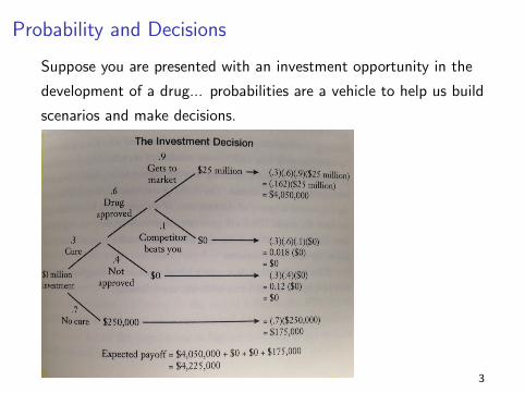
Suppose you are presented with an investment opportunity in the

development of a drug... probabilities are a vehicle to help us build

scenarios and make decisions.

3

Probability and Decisions

We basically have a new random variable, i.e, our revenue, with

the following probabilities...

Revenue P(Revenue)

$250,000 0.7

$0 0.138

$25,000,000 0.162

The expected revenue is then $4,225,000...

So, should we invest or not?

4

Back to Targeted Marketing

Should we send the promotion ???

Well, it depends on how likely it is that the customer will respond!!

If they respond, you get 40-0.8=$39.20.

If they do not respond, you lose $0.80.

Let’s assume your “predictive analytics” team has studied the

conditional probability of customer responses given customer

characteristics... (say, previous purchase behavior, demographics,

etc)

5

Back to Targeted Marketing

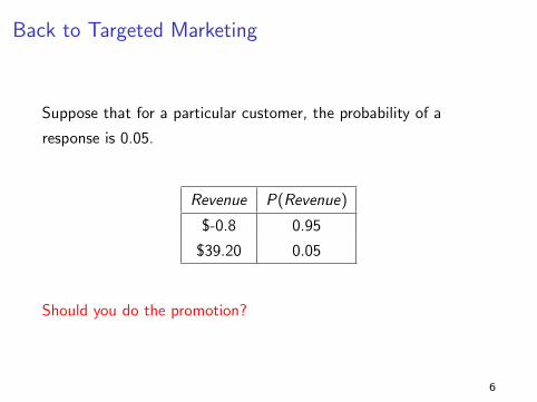
Suppose that for a particular customer, the probability of a

response is 0.05.

Revenue P(Revenue)

$-0.8 0.95

$39.20 0.05

Should you do the promotion?

6

Probability and Decisions

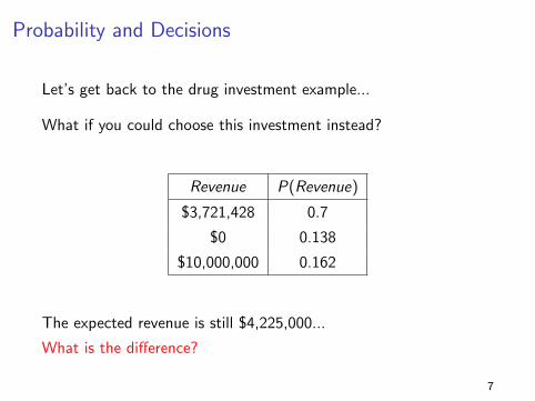
Let’s get back to the drug investment example...

What if you could choose this investment instead?

Revenue P(Revenue)

$3,721,428 0.7

$0 0.138

$10,000,000 0.162

The expected revenue is still $4,225,000...

What is the difference?

7

Mean and Variance of a Random Variable

The Mean or Expected Value is defined as (for a discrete X with n

possible outcomes):

E (X ) =n∑

i=1

Pr(X = xi )× xi

We weight each possible value by how likely they are... this

provides us with a measure of centrality of the distribution... a

“good” prediction for X !

8

Example: Mean and Variance of a Binary Random Variable

Suppose

X =

{1 with prob. p

0 with prob. 1− p

E (X ) =n∑

i=1

Pr(xi )× xi

= 0× (1− p) + 1× p

E (X ) = p

Another example: What is the E (Revenue) for the targeted

marketing problem?

9

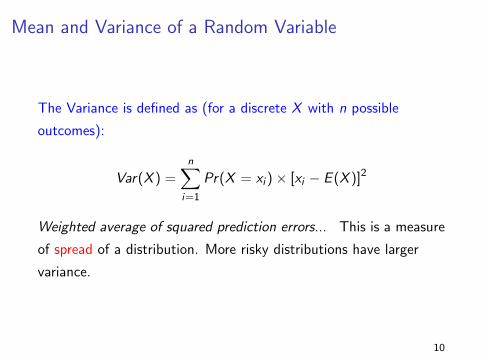
Mean and Variance of a Random Variable

The Variance is defined as (for a discrete X with n possible

outcomes):

Var(X ) =n∑

i=1

Pr(X = xi )× [xi − E (X )]2

Weighted average of squared prediction errors... This is a measure

of spread of a distribution. More risky distributions have larger

variance.

10

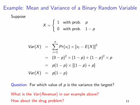
Example: Mean and Variance of a Binary Random Variable

Suppose

X =

{1 with prob. p

0 with prob. 1− p

Var(X ) =n∑

i=1

Pr(xi )× [xi − E (X )]2

= (0− p)2 × (1− p) + (1− p)2 × p

= p(1− p)× [(1− p) + p]

Var(X ) = p(1− p)

Question: For which value of p is the variance the largest?

What is the Var(Revenue) in our example above?

How about the drug problem? 11

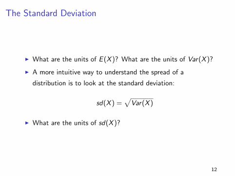
The Standard Deviation

I What are the units of E (X )? What are the units of Var(X )?

I A more intuitive way to understand the spread of a

distribution is to look at the standard deviation:

sd(X ) =√

Var(X )

I What are the units of sd(X )?

12

Mean, Variance, Standard Deviation: Summary

What to keep in mind about the mean, variance, and SD:

I The expected value/mean is usually our best prediction of

an uncertain outcome. (“Best” meaning closest in distance to

the realized outcome, for a particular measure of distance)

I The variance is often a reasonable summary of how

unpredictable an uncertain outcome is (or how risky it is to

predict)

I The standard deviation (square root of the variance) is

another reasonable summary of risk that is on a meaningful

scale.

13

Why expected values?

I When you have a repeated decision problem (or many

decisions to make), make decisions to maximize your

expected utility

I Utility functions provide a numeric value to outcomes; those

with higher utilities are preferred

I Profit/payoff is one utility function. More realistic utilities

allow for risk taking/aversion, but the concepts are the same.

14

Decision Trees

A convenient way to represent decision problems:

I Time proceeds from left to right.

I Branches leading out of a decision node (usually a square)

represent the possible decisions.

I Probabilities are listed on probability branches, and are

conditional on the events that have already been observed

(i.e., they assume that everything to the left has already

happened).

I Monetary values (utilities) are shown to the right of the end

nodes.

I EVs are calculated through a “rolling-back” process.

15

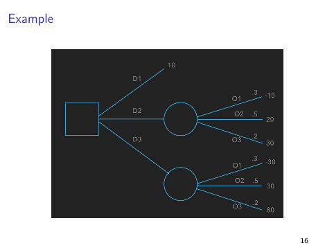
Example

16

Rolling back: Step 1

Calculate the expected value at each probability node:

E (Payoff | D2) = .3(−10) + .5(20) + .2(30) = 1317

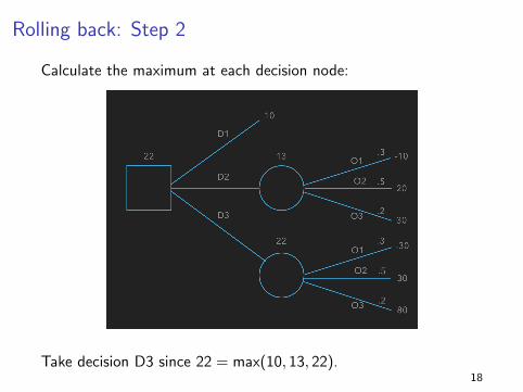
Rolling back: Step 2

Calculate the maximum at each decision node:

Take decision D3 since 22 = max(10, 13, 22).18

Sally Ann Soles’ Shoe Factory

Sally Ann Soles manages a successful shoe factory. She is

wondering whether to expand her factory this year.

I The cost of the expansion is $1.5M.

I If she does nothing and the economy stays good, she expects

to earn $3M in revenue, but if the economy is bad, she

expects only $1M.

I If she expands the factory, she expects to earn $6M if the

economy is good and $2M if it is bad.

I She estimates that there is a 40 percent chance of a good

economy and a 60 percent chance of a bad economy.

Should she expand?

19

E (expand) = (.4(6) + .6(2))− 1.5 = 2.1

E (don’t expand) = (.4(3) + .6(1)) = 1.8

Since 2.1 > 1.8, she should expand, right? (Why might she choose

not to expand?) 20

Sequential decisions

She later learns after she finishes the expansion, she can assess the

state of the economy and opt to either:

(a) expand the factory further, which costs $1.5M and will yield

an extra $2M in profit if the economy is good, but $1M if it is

bad,

(b) abandon the project and sell the equipment she originally

bought, for $1.3M – obtaining $1.3M, plus the payoff if she

had never expanded, or

(c) do nothing.

How has the decision changed?

21

Sequential decisions

22

Expected value of the option

The EV of expanding is now

(.4(6.5) + .6(2.3))− 1.5 = 2.48.

If the option were free, is there any reason not to expand?

What would you pay for the option? How about

E (new)− E (old) = 2.48− 2.1 = 0.38,

or $380,000?

23

What Is It Worth to Know More About an Uncertain

Event?

24

Value of information

I Sometimes information can lead to better decisions.

I How much is information worth, and if it costs a given

amount, should you purchase it?

I The expected value of perfect information, or EVPI, is the

most you would be willing to pay for perfect information.

25

Typical setup

I In a multistage decision problem, often the first-stage decision

is whether to purchase information that will help make a

better second stage decision

I In this case the information, if obtained, may change the

probabilities of later outcomes

I In addition, you typically want to learn how much the

information is worth

I Information usually comes at a price. You want to know

whether the information is worth its price

I This leads to an investigation of the value of information

26

Example: Marketing Strategy for Bevo: The Movie

UT Productions has to decide on a marketing strategy for it’s new

movie, Bevo. Three major strategies are being considered:

I (A) Aggressive: Large expenditures on television and print

advertising.

I (B) Basic: More modest marketing campaign.

I (C) Cautious: Minimal marketing campaign.

27

Payoffs for Bevo: The Movie

The net payoffs depend on the market reaction to the film.

28

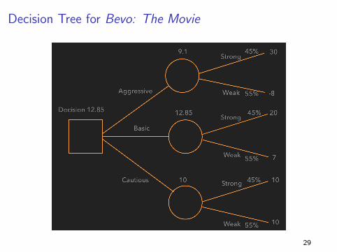
Decision Tree for Bevo: The Movie

29

Expected Value of Perfect Information (EVPI)

How valuable would it be to know what was going to happen?

I If a clairvoyant were available to tell you what is going to

happen, how much would you pay her?

I Assume that you don’t know what the clairvoyant will say and

you have to pay her before she reveals the answer

EVPI = (EV with perfect information) - (EV with no information)

30

Finding EVPI with a payoff table

The payoffs depend on the market reaction to the film:

I With no information, the Basic strategy is best: EV =

0.45(20) + 0.55(7) = 12.85

I With perfect info, select the Agressive strategy for a Strong

reaction and the Cautious strategy for a Weak reaction: EV =

0.45(30) + 0.55(10) = 19

I EVPI = 19− 12.85 = 6.15 31

Finding EVPI with a decision tree

I Step 1: Set up tree without perfect information and calculate

EV by rolling back

I Step 2: Rearrange the tree the reflect the receipt of the

information and calculate the new EV

I Step 3: Compare the EV’s with and without the information

32

Finding EVPI with a decision tree

33

What about imperfect information?

Suppose that Myra the movie critic has a good record of picking

winners, but she isn’t clairvoyant. What is her information worth?

34

The decision tree with imperfect information

How does this compare with the perfect information tree?We need to get the relevant conditional probabilities... 35

How good is the information?

Suppose that Myra the movie critic has a good record of picking

winners.

I For movies where the audience reaction was strong, Myra has

historically predicted that 70% of them would be strong.

I For movies where the audience reaction was weak, Myra has

historically predicted that 80% of them would be weak.

Remember that the chance of a strong reaction is 45% and of a

weak reaction is 55%.

36

Suppose S and W means the audience reaction was strong or

weak, respectively, and PS and PW means that Myra’s prediction

was strong or weak, respectively. Let’s translate what we know:

I For movies where the audience reaction was strong, Myra has

historically predicted that 70% of them would be strong.

P(PS |S) = .7, P(PW |S) = .3

I For movies where the audience reaction was weak, Myra has

historically predicted that 80% of them would be weak.

P(PW |W ) = .8, P(PS |W ) = .2

I The chance of a strong reaction is 45% and of a weak

reaction is 55%.

P(S) = .45, P(W ) = .55

37

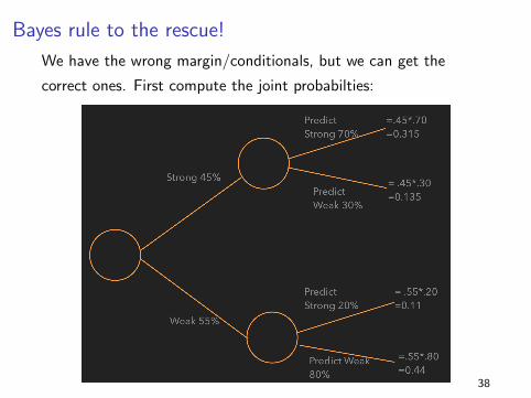
Bayes rule to the rescue!

We have the wrong margin/conditionals, but we can get the

correct ones. First compute the joint probabilties:

38

What distributions do we need?

The sequence is (Myra predicts) → (We decide)

First uncertain outcome in the new tree is Myra’s prediction, so we

need P(PS) and P(PW ) = 1− P(PS):

P(PS) = P(PS | S)P(S) + P(PS |W )P(W ) = (0.315+0.11) = 0.425

39

What conditionals do we need?

The sequence is (Myra predicts) → (We decide)

Next uncertain outcome is the true market response, so we need

P(S | PS) and P(W | PW ):

P(S | PS) =P(PS | S)P(S)

P(PS)= 0.315/0.425 = 0.741

P(W | PW ) =P(PW |W )P(W )

P(PW )= 0.44/(1− 0.425) = 0.765

40

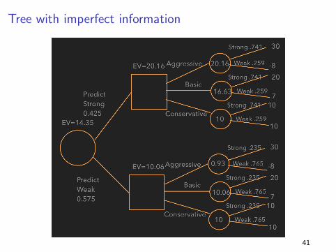
Tree with imperfect information

41

Myra’s information is worth paying for

It changes the decision and adds 14.35− 12.85 = 1.5 in value.

(Compare this to the 6.15 the clairvoyant’s prediction was worth.)

42

Things to remember about the value of information

I Perfect information is more valuable that any imperfect

information

I Information cannot have negative value

43

Decision trees: Summary

I Useful framework for simplifying some probability &

expectation calculations.

I “Under the hood” they are simply applications of conditional

probability and expectation!

I Specialized software exists for complicated trees (e.g.

Pallisade PrecisionTree in Excel or the free Radiant R

package) but the concepts are the same.

44

Combining random variables

We’ve seen how the expected value (our best prediction) and

variance/standard deviation (how risky our best prediction is)

help us think about uncertainty and make decisions in simple

scenarios

We need some more tools for thinking about multiple random

variables (sources of uncertainty)

45

Covariance

I A measure of dependence between two random variables...

I It tells us how two unknown quantities tend to move together:

Positive → One goes up (down), the other tends to go up

(down). Negative → One goes down (up), the other tends to

go up (down).

I If X and Y are independent, Cov(X ,Y ) = 0 BUT

Cov(X ,Y ) = 0 does not mean X and Y are independent

(more on this later).

The Covariance is defined as (for discrete X and Y ):

Cov(X ,Y ) =n∑

i=1

m∑j=1

Pr(xi , yj)× [xi − E (X )]× [yj − E (Y )]

I What are the units of Cov(X ,Y ) ?

46

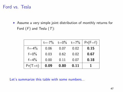
Ford vs. Tesla

I Assume a very simple joint distribution of monthly returns for

Ford (F ) and Tesla (T ):

t=-7% t=0% t=7% Pr(F=f)

f=-4% 0.06 0.07 0.02 0.15

f=0% 0.03 0.62 0.02 0.67

f=4% 0.00 0.11 0.07 0.18

Pr(T=t) 0.09 0.80 0.11 1

Let’s summarize this table with some numbers...

47

Example: Ford vs. Tesla

t=-7% t=0% t=7% Pr(F=f)

f=-4% 0.06 0.07 0.02 0.15

f=0% 0.03 0.62 0.02 0.67

f=4% 0.00 0.11 0.07 0.18

Pr(T=t) 0.09 0.80 0.11 1

I E (F ) = 0.12, E (T ) = 0.14

I Var(F ) = 5.25, sd(F ) = 2.29, Var(T ) = 9.76, sd(T ) = 3.12

I What is the better stock?

48

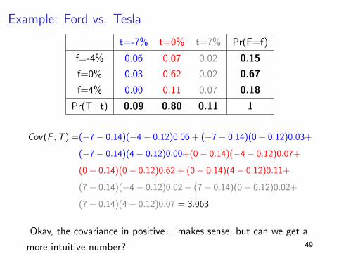
Example: Ford vs. Tesla

t=-7% t=0% t=7% Pr(F=f)

f=-4% 0.06 0.07 0.02 0.15

f=0% 0.03 0.62 0.02 0.67

f=4% 0.00 0.11 0.07 0.18

Pr(T=t) 0.09 0.80 0.11 1

Cov(F ,T ) =(−7− 0.14)(−4− 0.12)0.06 + (−7− 0.14)(0− 0.12)0.03+

(−7− 0.14)(4− 0.12)0.00+(0− 0.14)(−4− 0.12)0.07+

(0− 0.14)(0− 0.12)0.62 + (0− 0.14)(4− 0.12)0.11+

(7− 0.14)(−4− 0.12)0.02 + (7− 0.14)(0− 0.12)0.02+

(7− 0.14)(4− 0.12)0.07 = 3.063

Okay, the covariance in positive... makes sense, but can we get a

more intuitive number? 49

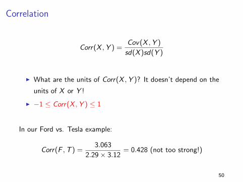
Correlation

Corr(X ,Y ) =Cov(X ,Y )

sd(X )sd(Y )

I What are the units of Corr(X ,Y )? It doesn’t depend on the

units of X or Y !

I −1 ≤ Corr(X ,Y ) ≤ 1

In our Ford vs. Tesla example:

Corr(F ,T ) =3.063

2.29× 3.12= 0.428 (not too strong!)

50

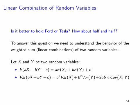
Linear Combination of Random Variables

Is it better to hold Ford or Tesla? How about half and half?

To answer this question we need to understand the behavior of the

weighted sum (linear combinations) of two random variables...

Let X and Y be two random variables:

I E (aX + bY + c) = aE (X ) + bE (Y ) + c

I Var(aX +bY +c) = a2Var(X )+b2Var(Y )+2ab×Cov(X ,Y )

51

Linear Combination of Random Variables

Applying this to the Ford vs. Tesla example...

I E (0.5F + 0.5T ) = 0.5E (F ) + 0.5E (T ) =

0.5× 0.12 + 0.5× 0.14 = 0.13

I Var(0.5F + 0.5T ) =

(0.5)2Var(F ) + (0.5)2Var(T ) + 2(0.5)(0.5)× Cov(F ,T ) =

(0.5)2(5.25) + (0.5)2(9.76) + 2(0.5)(0.5)× 3.063 = 5.28

I sd(0.5F + 0.5T ) = 2.297

so, what is better? Holding Ford, Tesla or the combination?

52

Risk Adjustment: Sharpe Ratio

The Sharpe ratio is a unitless quantity used to compare

investments:

(average return) - (return on a risk-free investment)

standard deviation of returns

Idea: Standardize the average excess return by the amount of risk.

(“Risk adjusted returns”)

Ignoring the risk-free investment, what are the Sharpe ratios for

Ford, Tesla, and the 50-50 portfolio?

53

Linear Combination of Random Variables

More generally...

I E (w1X1 + w2X2 + ...wpXp + c) =

w1E (X1) + w2E (X2) + ...+ wpE (Xp) + c =∑p

i=1 wiE (Xi ) + c

I Var(w1X1 + w2X2 + ...wpXp + c) = w21 Var(X1) + w2

2 Var(X2) +

...+w2pVar(Xp)+2w1w2×Cov(X1,X2)+2w1w3Cov(X1,X3)+

... =∑p

i=1 w2i Var(Xi ) +

∑pi=1

∑j 6=i wiwjCov(Xi ,Xj)

where w1,w2, . . . ,wp and c are constants

54