Jared Michael Darius - Liberty University
87
Running head: INNOVATIVE FORMULA SAE SUSPENSION DESIGN 1 The Design of an Innovative Automotive Suspension for Formula SAE Racing Applications Jared Michael Darius A Senior Thesis submitted in partial fulfillment of the requirements for graduation in the Honors Program Liberty University Spring 2019
Transcript of Jared Michael Darius - Liberty University

Running head: INNOVATIVE FORMULA SAE SUSPENSION DESIGN 1
The Design of an Innovative Automotive Suspension
for Formula SAE Racing Applications
Jared Michael Darius
A Senior Thesis submitted in partial fulfillment
of the requirements for graduation
in the Honors Program
Liberty University
Spring 2019

INNOVATIVE FORMULA SAE SUSPENSION DESIGN 2
Acceptance of Senior Honors Thesis
This Senior Honors Thesis is accepted in partial
Fulfillment of the requirements for graduation from the
Honors Program of Liberty University.
___________________________
Hector Medina, Ph.D.
Thesis Chair
___________________________
Thomas Eldredge, Ph.D.
Committee Member
___________________________
Timo Budarz, Ph.D.
Committee Member
___________________________
James H. Nutter, D.A.
Honors Director
___________________________
Date
INNOVATIVE FORMULA SAE SUSPENSION DESIGN 3
Abstract
This thesis details an analytical approach to an innovative suspension system design for
implementation to the Formula SAE collegiate competition. It focuses specifically on
design relating to geometry, mathematical modeling, energy element relationships, and
computer analysis and simulation to visualize system behavior. The bond graph approach
is utilized for a quarter car model to facilitate understanding of the analytical process,
then applied to a comparative analysis between two transverse half car models. The
second half car model contains an additional transverse linkage with a third damper, and
is compared against the baseline of the first half car model without the additional linkage.
The transverse third damper is an innovative design said to improve straight-line tire
contact during single-sided disturbance, help mitigate the adverse effects of squat and
dive, while not inhibiting the function of the anti-roll bar in cornering capability.
Additional work is done investigating an optimization of suspension geometry through
mathematical modeling in MATLAB of a four-bar linkage system. This code helps
visualize the complex motion of the upright and calculates the wheel camber rate and
variation to compare against tire data analysis to match maximum tire performance
characteristics with camber angle.
INNOVATIVE FORMULA SAE SUSPENSION DESIGN 4
Table of Contents
Chapter 1: Introduction/Background ............................................................................................... 6
Literature Review....................................................................................................................... 13
Transverse 3rd damper integration .......................................................................................... 13
Magnetorheological damper integration ................................................................................ 16
Chapter 2: Geometry Considerations ............................................................................................. 20
Tire Data Analysis ..................................................................................................................... 20
Roll center .............................................................................................................................. 26
Four-bar linkage motion analysis ........................................................................................... 29
Chapter 3: Energy and Behavioral Considerations ........................................................................ 35
Conventional Quarter Car Model Analysis ................................................................................ 36
Schematic ............................................................................................................................... 36
Bond Graph ............................................................................................................................ 37
Derivation of state space equations and matrix...................................................................... 37
Conventional Transverse Half Car Model Analysis .................................................................. 45
Schematic ............................................................................................................................... 46
Bond Graph ............................................................................................................................ 46
Derivation of state space equations and matrix...................................................................... 47
Introduction to Koenigsegg Design ........................................................................................... 54
Koenigsegg Design Transverse Half-Car Model Analysis ........................................................ 55
Schematic ............................................................................................................................... 55
Bond Graph ............................................................................................................................ 55
Derivation of state space equations and matrix...................................................................... 56
Discussion ...................................................................................................................................... 60
Semi-Active System Control with Magnetorheological Dampers ................................................. 61
Conclusion ..................................................................................................................................... 66

INNOVATIVE FORMULA SAE SUSPENSION DESIGN 5
Limitations and Future Work ......................................................................................................... 67
References ...................................................................................................................................... 68
Appendix A ................................................................................................................................ 70
Mass Spring Damper System: 2nd Order Differential Equation Development: ..................... 70
Appendix B ................................................................................................................................ 74
MATLAB Code Generated for Four-Bar Linkage Analysis .................................................. 74
Appendix C ................................................................................................................................ 77
MATLAB Code Generated for Dynamic Systems Vehicle Response Analysis .................... 77
Appendix D ................................................................................................................................ 87
Hand Calculations and Derivations of Dynamic Systems Analysis ...................................... 87
INNOVATIVE FORMULA SAE SUSPENSION DESIGN 6
Innovative Formula SAE Suspension Design
Chapter 1: Introduction/Background
Undoubtedly, suspension systems are critical to the dynamic performance of a
race car. From the word’s roots, it means literally to “suspend,” or keep something raised
from the ground. This is exactly what vehicle suspension systems do; the body and
chassis of a vehicle is kept suspended from the ground through a series of linkages and
connections to energy storage and dissipative elements, which control the contact
between the tires and the ground. In other words, springs (energy storage) and dampers
(energy dissipation) are mounted between the vehicle’s frame and control arms to
translate the weight of the vehicle through these elements and into the wheels, which
push down against the ground and by Newton’s 3rd law push back up against the wheels
to keep the car suspended. However, there is more to a suspension system than simply
keeping something raised above the ground – if this were the case then we could simply
use fixed non-compliant connections between the wheels and the frame to keep the frame
from dragging on the ground. The disadvantage of such a system comes when the wheels
hit a bump or pothole, and the entirety of that force is translated directly into the frame,
likely causing fracture and failure. To avoid this, springs were placed in the connection
between wheels and chassis so that when hitting a bump, some of that impact energy goes
into compressing and extending the springs which minimizes the energy absorption
required by the frame. Still, this caused another issue of riding discomfort as the springs
freely oscillate up and down until enough energy is naturally dissipated to return back to
a steady-state equilibrium position (which can take quite a while). Thus, another element
INNOVATIVE FORMULA SAE SUSPENSION DESIGN 7
was added to quickly dissipate the energy that causes prolonged oscillation – the damper.
However, not just any configuration of these elements will suffice; there are specific
ratios and combinations of mass, spring stiffness, and damping coefficients that yield a
comfortable riding experience and maintain the optimal contact patch between each of
the tires and the road.
In researching how to design a racing vehicle’s suspension system, nearly every
source has something different to say about how and where to begin. A vehicle’s
suspension system is the most important subsystem of a dynamic performance racing
vehicle. To narrow the scope of this investigation, this research is focused on ways in
which the suspension system of a FSAE racing vehicle can be optimized. Thus, the
results of this investigation may be directly applied to the design of Liberty University’s
Formula SAE team. The suspension system is where the rubber meets the road, so the
design is focused on best controlling that physical interface across a range of loading
conditions. In dynamic racing applications, as the sprung mass of the vehicle chassis and
driver are being accelerated they produce a reactive force that must be balanced and
utilized to both maintain and increase traction and contact with the road, to maximize the
ability of the wheels to keep a secure grip and maintain as high a speed as possible
without sliding off the track.
As such, a suspension system is designed with two primary purposes in mind; first
to accelerate from a stop to top speed and decelerate to a stop as quickly as possible in a
straight line, and second to maintain the highest speed possible through a turn. In the first
of these, the goal is to allow the vehicle’s inertia to cause a controlled “squat” on the

INNOVATIVE FORMULA SAE SUSPENSION DESIGN 8
power producing wheels as the effective center of mass is shifted towards the rear wheels
producing a greater normal force over the rear wheels to increase the possible force of
friction before slipping. For the second of these, the goal is similar, in that the inertia and
momentum of the sprung mass must be controlled from excessive roll when changing
yaw as the vehicle travels through a turn (See Figure 1).
Figure 1: Axis definition and nomenclature of rotational movements about each axis.
When turning, the center of mass is effectively shifted towards the outside of the
turn, putting more normal force on those outside wheels (called load transfer). If
excessive this can be dangerous, and potentially cause the vehicle to either slip from the
track or roll completely if the center of mass is displaced beyond the limits of the outer
wheels from too much side loading. The degree of body roll is controlled by the stiffness
of the springs and anti-roll bar (essentially a torsional spring) in the suspension, while the
dampers are designed to control a rapid and hard-hitting force like a bump or pothole in
the road, to dissipate the energy of the oscillatory result of a wheel displacement due to
the nature of springs. Both of these energy components (the springs and dampers) in a

INNOVATIVE FORMULA SAE SUSPENSION DESIGN 9
vehicle’s suspension system are of critical importance to control the vehicle’s dynamic
behavior. Frequency response analysis may be done with a variety of input parameters to
find coefficients that are best optimized for the vehicle’s performance. Such analysis is
demonstrated in the latter sections of this investigation. However, another important
component of suspension design is the system geometry, providing the lengths and
connection angles of the linkages between wheels and chassis. The conventional
suspension system referenced here is the common double wishbone suspension, pictured
in Figure 2, as found in most performance vehicles. It is acknowledged that there is a
plethora of various types of suspension such as MacPherson Strut, leaf spring, and
trailing arm to name a few, but within the field of racing the double wishbone is the most
widely implemented design.
Figure 2: Double wishbone suspension system, partial car model.
Upper Wishbone Arm
Lower Wishbone Arm
Spring
Damper
See
Fig
ure
3
Coilover
INNOVATIVE FORMULA SAE SUSPENSION DESIGN 10
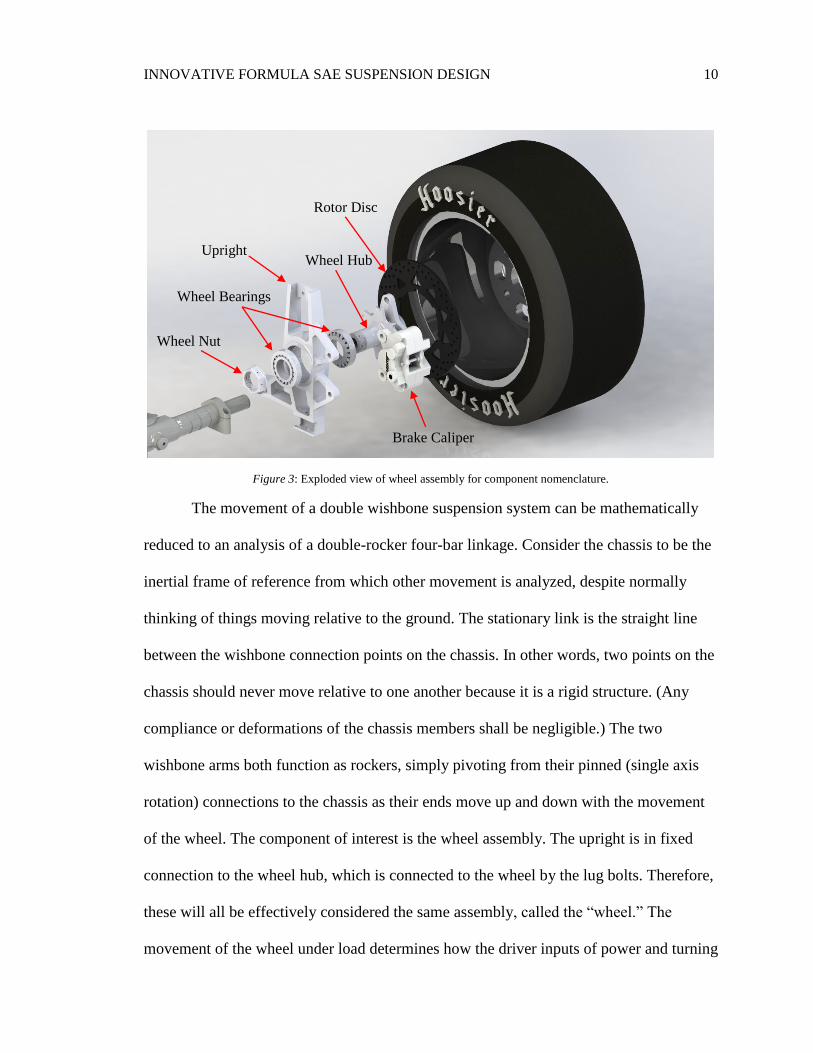
Figure 3: Exploded view of wheel assembly for component nomenclature.
The movement of a double wishbone suspension system can be mathematically
reduced to an analysis of a double-rocker four-bar linkage. Consider the chassis to be the
inertial frame of reference from which other movement is analyzed, despite normally
thinking of things moving relative to the ground. The stationary link is the straight line
between the wishbone connection points on the chassis. In other words, two points on the
chassis should never move relative to one another because it is a rigid structure. (Any
compliance or deformations of the chassis members shall be negligible.) The two
wishbone arms both function as rockers, simply pivoting from their pinned (single axis
rotation) connections to the chassis as their ends move up and down with the movement
of the wheel. The component of interest is the wheel assembly. The upright is in fixed
connection to the wheel hub, which is connected to the wheel by the lug bolts. Therefore,
these will all be effectively considered the same assembly, called the “wheel.” The
movement of the wheel under load determines how the driver inputs of power and turning
Brake Caliper
Wheel Hub Upright
Wheel Bearings
Wheel Nut
Rotor Disc

INNOVATIVE FORMULA SAE SUSPENSION DESIGN 11
connect to the road to provide feedback and give direction to the driver’s movements.
Unless a double wishbone suspension geometry is designed to be a perfect parallelogram,
the wheel must change its angle as it translates up and down, as demonstrated by the
four-bar linkage analysis. Therefore, the wheel is in complex movement, both translating
and rotating relative to the chassis. This has a direct effect on camber angle (See Figure
4), which is a key parameter within the calculations of a wheel’s contact patch. The
contact patch ultimately determines the maximum friction force capable of being
transmitted between the tire and road before slipping.
Figure 4: Visual depiction of camber angle.
Generally, it is most desirable for a vehicle to have neutral camber in wheel
alignment for even tread wear and maximum contact patch area during normal driving.
However, given that racing is not normal driving, a perfectly neutral camber is not always
desirable because it does not yield a maximum contact patch area when the driver takes
very hard turns and the wheels are displaced according to their suspension geometry path.
In fact, it is better to create negative camber on the wheels on the outside of a turn, as the
wheel is forced upward by the increased effective load it is supporting through its springs
causing them to compress. The precise desired angle of negative camber is more difficult

INNOVATIVE FORMULA SAE SUSPENSION DESIGN 12
to calculate, but it is important to visualize the path of the wheel and camber angle
throughout projected wheel displacement (See Figure 5).
Figure 5: Depiction of jounce and rebound relative to spring compression and extension.
Therefore, I created a program in MATLAB (see Four-bar Linkage Motion
Analysis Section) that could plot the movement of a four-bar linkage through a range of
movement, inputting custom lengths of all the links. In this way, with the design of the
FSAE vehicle in mind, dimensions directly relating to desired variables of the vehicle
could be tested and manipulated. These included track width, ride height, and chassis
frame members to design where the suspension components could be mounted, and what
their corresponding lengths should be to have a desired complex path demonstrated by
the wheel through jounce primarily, but also in rebound of the wheel.
With all the interacting factors that need to be considered during suspension
design, it makes suspension optimization a challenging and rewarding field when done
right. Further, given the many interdependent variables that may be altered, it leaves

INNOVATIVE FORMULA SAE SUSPENSION DESIGN 13
room for seemingly infinite design possibilities, always leaving room for improvement
and development.
Literature Review
Transverse 3rd damper integration. Certainly the most ambitious innovation to
racing vehicle design discussed here is the implementation of a third damper mounted
transversely between both the front and rear pairs of wheels. This design was pioneered
by Koenigsegg; a company whose mission is to take areas of compromise in vehicle
design and find ways to minimize or eliminate such compromise. In suspension design,
nearly everything is a tradeoff. Koenigsegg saw one of these areas, in which superior
cornering capability came at the cost of driver comfort and straight-line traction – and
decided to do something about it.
There are many types of vehicle racing. As a result, the racing vehicle is designed
very differently to optimize the conditions it is subjected to. For example, a drag racer
and a Formula 1 vehicle are each very successful in straight-line and dynamic circuit
tracks respectively, but put one in the other’s race, and it will fail miserably against the
competition. An engineer’s job is to utilize physics and mathematics, with a scientific
approach, to understand as much as possible about the materials and forces at play to
make the greatest use of the strengths and minimize the weaknesses in a design. The
incorporation of a third damper is most effective in the design of a suspension intended
for a more dynamic circuit – like those raced by Formula 1 vehicles. This racing setting
demands that a vehicle be able to corner exceptionally well, but it cannot come at the cost
of general traction and driver comfort, which is critical in endurance events.

INNOVATIVE FORMULA SAE SUSPENSION DESIGN 14
A traditional approach to this trade-off dilemma is to tune the stiffness of the anti-
roll bar, finding a sweet spot based on mathematical modeling and on-track testing so that
it is as stiff as allowable without too much compromise in traction. This traction
compromise comes from the fact that the anti-roll bar is the only direct connection
between two otherwise independently suspended wheels, serving to force both wheels to
move in the same direction to reduce the body roll generated by one wheel being forcibly
compressed on the outside of a turn when cornering from lateral load transfer. As this
outside wheel is compressed under greater load, a torsion is generated in the anti-roll bar,
which is then applied to the inside wheel, compressing it as well and therefore allowing
the chassis to come back closer to the road on the inside and balance out the roll.
However, as useful as it is to balance out roll in a corner as one wheel imparts a
force on the other through the torsion of the anti-roll bar, this same tendency is
detrimental to traction in a straight line when bumps on the track surface cause wheel
displacements on one side of the vehicle that are then also imparted to the other side.
When this happens, a wheel is being unnecessarily “lifted” from the road when the
opposite wheel hits a bump. (More realistically the wheel is not fully lifted from the
pavement, there is only a reduction in the vertical load applied to the wheel.) Such a
reduction in vertical load means that the maximum possible friction force between the
tire and road is significantly reduced, because 𝑓𝑓 = 𝜇𝑁 and 𝑁 is directly proportional to
𝑓𝑓 (where 𝑓𝑓 is the friction force, 𝜇 is the friction coefficient, and 𝑁 is the normal force).
A third damper, however, mounted transversely across the width of the vehicle
similarly to the anti-roll bar establishes a second connection between the two otherwise
INNOVATIVE FORMULA SAE SUSPENSION DESIGN 15
independently suspended wheels. This time, there is an energy dissipating effect from the
damper, as a force imparted on either wheel is translated by a pushrod into a
displacement of the piston within the damper cylinder, effectively converting the kinetic
energy from the motion of the wheel into heat as the viscous damping fluid is forced
through the capillary holes of the piston head creating viscous friction within the fluid.
The damping coefficient of energy dissipation is controllable by the viscosity of the
damping fluid, either by filling the chamber with different fluids, or utilizing a fluid
whose viscosity can be altered. Magnetorheological fluids are capable of this by the
introduction of a magnetic field within the fluid to change viscosity, and will be
discussed in the following section.
With an energy dissipating element, the disturbances felt from one wheel to
another are greatly reduced, while cornering capability is not impeded. The damper
responds effectively to rapid displacements as the damping force is proportional to the
velocity of the internal piston, and permits the anti-roll bar to accomplish its purpose in
more sustained displacements such as those of cornering. Therefore, a stiff anti-roll bar
may be implemented to improve cornering capability, while the negative effects of
opposite wheel displacements and loss of traction are mitigated by the dissipation of
those forces through the transversely mounted third damper, and driver comfort and road-
feel are also improved. Further, with the implementation of magnetorheological fluid and
sensor feedback for automated and calculated control of the damping coefficient, the
control of the entire suspension system is taken to a new level, and vehicle handling is
more capable than ever before.

INNOVATIVE FORMULA SAE SUSPENSION DESIGN 16
Magnetorheological damper integration. Conventional dampers are constructed with
two basic components, the piston and cylinder. (See Figure 6) Though there are many
variations of form, including monotube, twin tube, internal bypass and more, it serves the
same purpose. The damper’s function is to dissipate energy, as a displacement force
either in tension or compression from the kinetic energy of wheel movement displaces
the piston, and is converted into heat within the hydraulic fluid by way of viscous
friction. That heat then slowly moves out into the environment by conduction to
connected parts or is carried away into the air as forced convection removes heat energy.
Figure 6: Cutaway view of conventional damper, twin-tube model.
As the piston is displaced within the hydraulic fluid, it increases pressure within
the hydraulic fluid on the compression side. This pressure is allowed to reach equilibrium
with the side opposite the piston by designing tight passages for the hydraulic fluid to
flow either around the sides of the piston at the walls of the cylinder, or through small

INNOVATIVE FORMULA SAE SUSPENSION DESIGN 17
holes in the piston head. It takes significant energy to force a viscous fluid through these
tight passages, and the viscous shearing happening within the fluid heats it up.
Dampers exist to control the repeated oscillations that would otherwise be present
from suspending the chassis on springs. Engineers tune the damping coefficient to a
specific value to establish an underdamped, critically damped, or overdamped system. A
simplified model of the system behavior can be easily interpreted from the plots of a
second order differential equation of the following form:
𝐹(𝑥) = 𝑚�̈� + 𝑏�̇� + 𝑘𝑥 (1)
In which 𝑚 represents the sprung mass, 𝑏 is the damping coefficient, and 𝑘 is the spring
constant. A derivation of this mass-spring-damper model is given in Appendix A for
further exploration, but the plot shown by Figure 7 reveals the behaviors possible by
tuning these three coefficients. The parameter zeta taken from that derivation is the
damping ratio, defined such that the system is critically damped when zeta equals one.
𝜁 =𝑏
𝑏𝑐=
𝑏
2𝑚𝜔𝑛=
𝑏
2𝑚√𝑘𝑚
(2)
Figure 7: Oscillatory behavior control of mass-spring-damper system by tuning of zeta parameter.
INNOVATIVE FORMULA SAE SUSPENSION DESIGN 18
Realistically however, this tuning process can be very laborious and time consuming to
make even small changes. Damping coefficients may be changed either by altering the
viscosity of the hydraulic fluid or altering the passages through which it must travel when
under pressure from the piston. This means disassembling the damper to either drain and
replace the hydraulic fluid for one with a different viscosity, or exchanging washers on
the piston head to change fluid flow through the passages. With sufficient data from field
testing we are able to very precisely predict and measure these damping coefficients.
However, there exists a much more versatile means of changing the behavior of a
damper.
Magnetorheological fluid is a fluid with iron particles in it that responds to a
magnetic stimulus, changing shape and/or viscosity. Engineers have implemented the use
of magnetorheological fluid within dampers by adding iron particles to hydraulic fluid,
such that when a magnetic field is induced within the fluid, it causes these iron particles
to align themselves. This particle alignment increases the viscosity of the fluid by making
it more resistant to deformation by shear stress. The magnetic field is generated by a coil
of wire running perpendicular to the length of the cylinder that has electric current sent
through it. Ampere’s Law dictates that the magnitude of the magnetic field generated
around a current carrying wire is proportional to the current in the wire. In this way, as
magnetorheological fluid viscosity is proportional to the strength of the magnetic field, so
it is also proportional to the magnitude of the current sent through the wires. This kind of
damper is pictured in Figure 8.

INNOVATIVE FORMULA SAE SUSPENSION DESIGN 19
Figure 8: Cutaway view of magnetorheological damper functionality.
Each year more sensors are being placed on various components within a vehicle
to have their data fed through the vehicle’s ECU for automatic adjustments based on
programmed code. The capacity for rapid tuning and real-time adjustment has
revolutionized the racing industry. With magnetorheological dampers, the effective
damping coefficient can be changed a fraction of a second after hitting a bump, or as the
brakes are being pressed to work against vehicle dive. In fact, Koenigsegg has their
dampers networked so as to be able to make remote adjustments to any of their cars at
any time wherever they are in the world, quickly enough to aid the vehicle as it races
along a track. Hydraulic fluid viscosity adjustments as rapid as current may be sent
through a wire is changing the way the racetrack is approached to optimize every second
of tire contact with the road through accelerations, corners, banks, and more.
Fluid
Flow
Fluid
Flow
INNOVATIVE FORMULA SAE SUSPENSION DESIGN 20
Further, to demonstrate the superior adjustability of magnetorheological dampers,
magnetorheological dampers have been designed with current carrying wires wound in
opposite directions and timed such that the residual coil inductance from the magnetic
field generated by the first coil is negated by the second. For example, the first coil
carrying electric current induces a magnetic field, aligning iron particles in the fluid.
When the viscosity is desired to be lower however, power is decreased or shut off to the
first coil, but it takes a fraction of a second for the magnetic field to dissipate due to
residual eddy currents caused by inductance, meaning that those aligned iron particles are
not yet released from their positions in the fluid so the viscosity takes time to drop down
to a lesser value. These eddy currents are counteracted by adding a second coil to the
damper so that as the first is being shut off, the second set activates and produces a
magnetic field in the opposite direction working to immediately disrupt the field that
existed and scatter the aligned ferrous particles, only activating long enough to disrupt the
effects of inductance from the first coil and then shutting off before realigning the
particles within a new magnetic field orientation.
Chapter 2: Geometry Considerations
Tire Data Analysis
A racing vehicle’s suspension system was stated as the subsystem where the
rubber meets the road, and that is exactly the location where the definition of suspension
geometry must begin. Professional racing teams spend substantial money on tire testing
with carefully calibrated machines. The data from tire testing can be analyzed to
determine the optimum orientation of the tire for given loading scenarios, which then

INNOVATIVE FORMULA SAE SUSPENSION DESIGN 21
determine how the wheel path should be constrained by the placement of suspension
linkages. For example, in a cornering scenario if the outside front wheel is considered, it
experiences a greater vertical load (due to load transfer from centripetal acceleration), as
well as a significant lateral load which directly correlates to the friction force that keeps
the wheel from sliding on the pavement. Many racing tires can increase their lateral load
capacity in a corner if there is some negative camber gain to angle the tire against the
pavement. However, too much camber can be even worse than none at all. A number of
years ago the Tire Test Consortium (TTC) was founded to provide a database for
Formula SAE students to access and retrieve this data to analyze for suspension design.
This database details exactly the test procedures that govern each set of data for proper
interpretation, and includes more than a dozen variables. It is the student’s job to select a
tire compound and dimensions, and get to work analyzing hundreds of thousands of lines
of data to make useful plots that will tell how the tire can best perform in the expected
racing conditions. The first of these plots is Slip Angle vs. Lateral Load. Slip angle is
understood according to Figure 9 as the angle difference between the steered intended
angle, and the actual traveled angle due to tire deformation at the contact patch.
Figure 9: Definition of slip angle; a result of applied lateral load deforming the tire at the contact patch.
INNOVATIVE FORMULA SAE SUSPENSION DESIGN 22
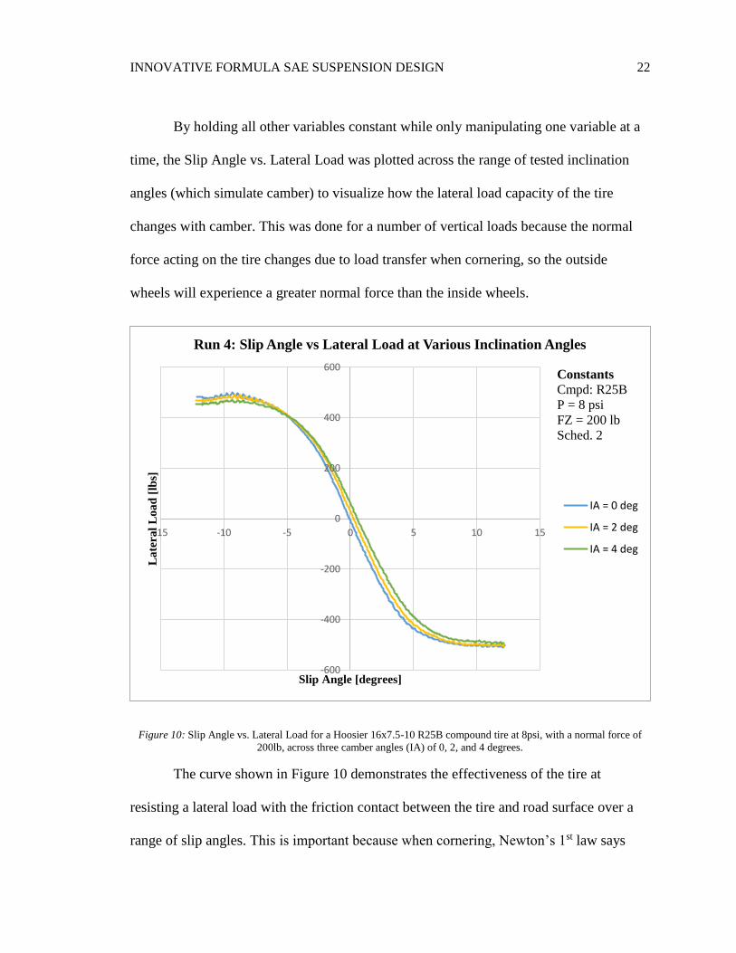
By holding all other variables constant while only manipulating one variable at a
time, the Slip Angle vs. Lateral Load was plotted across the range of tested inclination
angles (which simulate camber) to visualize how the lateral load capacity of the tire
changes with camber. This was done for a number of vertical loads because the normal
force acting on the tire changes due to load transfer when cornering, so the outside
wheels will experience a greater normal force than the inside wheels.
Figure 10: Slip Angle vs. Lateral Load for a Hoosier 16x7.5-10 R25B compound tire at 8psi, with a normal force of
200lb, across three camber angles (IA) of 0, 2, and 4 degrees.
The curve shown in Figure 10 demonstrates the effectiveness of the tire at
resisting a lateral load with the friction contact between the tire and road surface over a
range of slip angles. This is important because when cornering, Newton’s 1st law says
-600
-400
-200
0
200
400
600
-15 -10 -5 0 5 10 15
La
tera
l L
oa
d [
lbs]
Slip Angle [degrees]
Run 4: Slip Angle vs Lateral Load at Various Inclination Angles
IA = 0 deg
IA = 2 deg
IA = 4 deg
Constants
Cmpd: R25B
P = 8 psi
FZ = 200 lb
Sched. 2

INNOVATIVE FORMULA SAE SUSPENSION DESIGN 23
that the vehicle will tend to continue going straight, unless accelerated towards the center
of curvature dictated by turning the steering wheel. The centripetal force generated that
pushes the car towards the center of curvature is the friction force acting between the tires
and road surface. The greater the friction capacity at this contact patch, the more
centripetal force can be generated to take turns at higher speeds. The negatively sloped
linear portion in the middle means that the tire is effectively resisting lateral loads; for
small slip angles the tire linearly increases in lateral load capacity. However, when the
curve begins to plateau at either end, this shows that the lateral load capacity of the tire is
tapering to its limit at high slip angles, so when the curve goes flat the tire has lost grip on
the road and will begin to slide across the pavement because the frictional force is not
enough to resist the lateral load from centripetal acceleration. In Figure 10 one can
clearly see that with different camber angles, the curve changes slightly and lateral load
capacity changes. In fact, it appears in this plot that the camber angle of zero (refer to
Figure 4) has the greatest peak lateral load capacity, but in the linear range the higher
camber angles have a greater lateral load. However, the answer is far from being
reached; these tires must be tested for various compounds, pressures, and normal forces
at the very least before being able to determine the desired camber change with wheel
travel for the suspension geometry. Figure 11 shows the comparison between two
different tire compounds, R25B and LCO, of the same tire dimensions.

INNOVATIVE FORMULA SAE SUSPENSION DESIGN 24
Figure 11: Comparison of R25B and LCO tire compounds at 8psi, camber of 2 degrees, and 200lb normal force.
According to Figure 11, it would appear that the LCO compound is the clear
winner with the higher peak lateral load capacity in the same conditions. However,
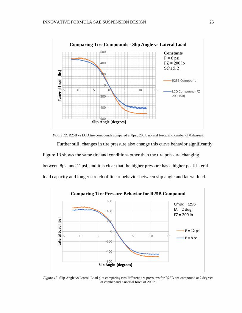
Figure 12 plots the same two tires with the same pressure and normal force, simply at a
camber of zero degrees, and the R25B compound takes the lead with a higher peak lateral
load capacity and a longer stretch of linear behavior in the curve.
-600
-400
-200
0
200
400
600
-15 -10 -5 0 5 10 15
La
tera
l L
oa
d [
lbs]
Slip Angle [degrees]
Comparing Tire Compounds - Slip Angle vs Lateral Load
LCO Compound
R25B Compound
FZ = 200 lbP = 8 psiIA = 2 deg
INNOVATIVE FORMULA SAE SUSPENSION DESIGN 25
Figure 12: R25B vs LCO tire compounds compared at 8psi, 200lb normal force, and camber of 0 degrees.
Further still, changes in tire pressure also change this curve behavior significantly.
Figure 13 shows the same tire and conditions other than the tire pressure changing
between 8psi and 12psi, and it is clear that the higher pressure has a higher peak lateral
load capacity and longer stretch of linear behavior between slip angle and lateral load.
Figure 13: Slip Angle vs Lateral Load plot comparing two different tire pressures for R25B tire compound at 2 degrees
of camber and a normal force of 200lb.
-600
-400
-200
0
200
400
600
-15 -10 -5 0 5 10 15
La
tera
l L
oa
d [
lbs]
Slip Angle [degrees]
Comparing Tire Compounds - Slip Angle vs Lateral Load
R25B Compound
LCO Compound (FZ200,150)
Constants
P = 8 psi
FZ = 200 lb
Sched. 2
-600
-400
-200
0
200
400
600
-15 -10 -5 0 5 10 15
Late
ral L
oad
[lb
s]
Slip Angle [degrees]
Comparing Tire Pressure Behavior for R25B Compound
P = 12 psi
P = 8 psi
Cmpd: R25BIA = 2 degFZ = 200 lb

INNOVATIVE FORMULA SAE SUSPENSION DESIGN 26
Therefore, without detailing the entirety of the tire analysis process, the previous
few plots should be sufficient to demonstrate the complexity in objectively defining the
desired camber rate in relation to vertical and lateral loads. Once sufficient analysis has
been done to make an argument for a specific camber rate limitation based on expected
wheel travel, the control arms in a double-wishbone system must then be designed
accordingly to yield such a camber rate with the expected wheel travel occurring during
lateral load transfer of cornering. The resulting camber at the maximum jounce position
during a cornering scenario must be a summation of both the ideal camber from slip
angle vs lateral load curves to maximize lateral load capacity, as well as the angle of
body roll resulting from the difference in spring compression on opposite sides of the car.
In this way, if the tire data shows peak lateral load capacity at 1.5 degrees of camber, and
the body rolls 1 degree in cornering from load transfer, the suspension geometry should
provide a total camber of 2.5 degrees at the wheel deflection expected in the same
cornering scenario.
Roll center. The roll center is the location about which the sprung mass will
rotate when experiencing body roll when cornering, and is one of the first things that
must be defined when designing suspension geometry. The ratio of the height of the roll
center relative to the height of the vehicle’s center of gravity determines the percentage of
anti-roll. Anti-roll is a measure of how much of the roll forces are reacted by the control
arms rather than the springs and dampers. Figure 14 shows a SolidWorks sketch of a
front view cross-section of the vehicle to place dimensions on things that would not
change, with extended lines to find the location of the instantaneous center of rotation of

INNOVATIVE FORMULA SAE SUSPENSION DESIGN 27
a wheel (IC). Then a line from the center of the tire contact with the road to the IC
location is drawn. The point where this line crosses the vertical line passing through the
center of gravity (assuming a laterally symmetric vehicle mass distribution) yields the
location of the roll center (RC). The distance between the center of gravity and the roll
center is the leverage of the roll moment. The closer they are together, the less body roll
is experienced with the same force, thus increasing anti-roll geometry by putting a greater
proportion of force into the control arms. However, while less body roll is generally a
good thing, it also leaves less room for control of the movement of the sprung mass
through the springs and dampers. A general range within the racing industry is about 15
to 30% anti-roll.
Figure 14: SolidWorks sketch to plan out roll center (RC) calculations. IC = instantaneous center, CG = center of
gravity.
RC
IC CG

INNOVATIVE FORMULA SAE SUSPENSION DESIGN 28
Figure 15: SolidWorks model front view of suspension system shown to match the geometry of the sketch in Figure 14.
The horizontal location of the instantaneous center along the line generated by the
center of the tire contact and the roll center is still variable at this point. Moving the IC
will adjust the mounting locations of the control arms to the frame, and therefore change
the relative lengths of the control arms. Both these adjustments have direct effects on the
path that the wheel travels in jounce and rebound. Not only are the arcs that each rocker
linkage makes changed, but the equilibrium position of the system relative to the angle
from the horizontal of the control arms is also changed with a new IC location. Therefore,
a means of visualizing the direct effects of these changes on camber rate was necessary,
and led to the creation of a code in MATLAB to solve the four-bar linkage equations and
make helpful plots.

INNOVATIVE FORMULA SAE SUSPENSION DESIGN 29
Four-bar linkage motion analysis. Concurrently with the RC calculations, when
mounting positions for the control arms were found that gave the desired percentage of
anti-roll, the suspension geometry then had to pass the camber variation test. A
MATLAB program was generated to yield the changes in camber angle over a length of
wheel travel of a double-wishbone suspension system, analyzing the system as a four-bar
linkage. Figure 16 represents the vector analysis notation to locate the points in the
linkage system as they move from a changing 𝜃2 input. The following Figures Figure 16
through Figure 20 demonstrate the final decided geometry for the rear suspension, having
determined an IC location that yields a desired camber change through wheel travel.
Figure 16: Four-bar linkage system defined by vectors and variables from which MATLAB variables were generated
for suspension camber analysis.
The mathematical analysis required to solve this system is not highly relevant to
suspension design, but can be found within the code for the MATLAB program in
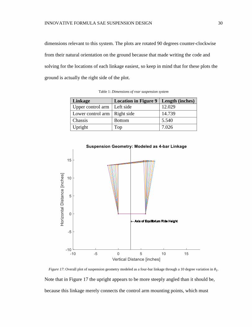
Appendix B. The first plot shown by Figure 17 shows a shape very similar to the one
seen in Figure 16, but also shows the instantaneous placement of all the linkages over a
𝜃2 variation of 10 degrees. This 10-degree change simulates the maximum desired wheel
travel (and minimum required travel) starting from one inch in rebound, passing the
equilibrium position, and extending to 1 inch in jounce. Table 1 gives important
INNOVATIVE FORMULA SAE SUSPENSION DESIGN 30
dimensions relevant to this system. The plots are rotated 90 degrees counter-clockwise
from their natural orientation on the ground because that made writing the code and
solving for the locations of each linkage easiest, so keep in mind that for these plots the
ground is actually the right side of the plot.
Table 1: Dimensions of rear suspension system
Linkage Location in Figure 9 Length (inches)
Upper control arm Left side 12.029
Lower control arm Right side 14.739
Chassis Bottom 5.540
Upright Top 7.026
Figure 17: Overall plot of suspension geometry modeled as a four-bar linkage through a 10 degree variation in 𝜃2.
Note that in Figure 17 the upright appears to be more steeply angled than it should be,
because this linkage merely connects the control arm mounting points, which must
INNOVATIVE FORMULA SAE SUSPENSION DESIGN 31
account for the Kingpin inclination angle. The resultant angle of the wheel is 8.3 degrees
different than that of the inclination angle, such that at the equilibrium ride height
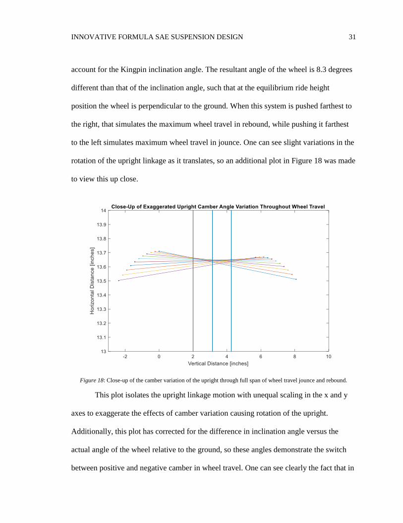
position the wheel is perpendicular to the ground. When this system is pushed farthest to
the right, that simulates the maximum wheel travel in rebound, while pushing it farthest
to the left simulates maximum wheel travel in jounce. One can see slight variations in the
rotation of the upright linkage as it translates, so an additional plot in Figure 18 was made
to view this up close.
Figure 18: Close-up of the camber variation of the upright through full span of wheel travel jounce and rebound.
This plot isolates the upright linkage motion with unequal scaling in the x and y
axes to exaggerate the effects of camber variation causing rotation of the upright.
Additionally, this plot has corrected for the difference in inclination angle versus the
actual angle of the wheel relative to the ground, so these angles demonstrate the switch
between positive and negative camber in wheel travel. One can see clearly the fact that in

INNOVATIVE FORMULA SAE SUSPENSION DESIGN 32
jounce the wheel is being forced towards increasingly negative camber. When cornering,
the lateral load applied to the tires causes them to deform as friction between the road and
tire pushes the tire towards the center of curvature. However, this friction force causes
deformation of the tire and changes the shape of the contact patch. A negative camber on
the outside wheel when cornering helps to counteract the loss of contact patch area, such
that tire deformations create a fuller contact patch. The full effects of this concept are
investigated through empirical testing of tires and plotting the collected data to visualize
such relationships. Though Figure 18 helps to show that there exists camber variation
with wheel travel, and that it makes a switch by becoming more negatively cambered
with jounce travel, we need to know just how much camber there is. With some more
calculations in MATLAB, Figure 19 shows exactly that.
Figure 19: Calculated camber angle of the wheel versus the theta 2 input to the four-bar linkage system, causing wheel
travel.

INNOVATIVE FORMULA SAE SUSPENSION DESIGN 33
It is evident from this graph that despite the exaggerated visual in Figure 18, there
is in fact very little camber variation with wheel travel. This is desired, because more
than just a few degrees of camber change can drastically change the way that the tire
interacts with the road and responds to various loads. At the equilibrium ride height
position, which the wheels will be at when driving in a straight line (without intense
launch and braking forces) the best contact patch is made when the tires are perpendicular
to the road surface. This is evident here by the camber angle of zero degrees at the middle
of wheel travel (when 𝜃2 is about 95 degrees). During cornering or launch when the
wheels are pushed up into jounce, the camber increases to about 1.25 degrees of negative
camber, and similarly in rebound.
Figure 20: Horizontal displacement of wheel center through vertical wheel travel.

INNOVATIVE FORMULA SAE SUSPENSION DESIGN 34
One final consideration is the amount of scrub the tire experiences through wheel
travel. Plotted in Figure 20 is the wheel center as it moves horizontally while translating
vertically during wheel travel. Scrub is a measure of the lateral distance that the center of
the tire translates laterally due to its wheel travel path. More scrub causes more drag and
resistance on the tires which takes energy away from the vehicle that could be forward
velocity. As shown in Figure 20 there is very little scrub, with maximum displacement
less than 0.10 inches, further proving the success of this geometry.
INNOVATIVE FORMULA SAE SUSPENSION DESIGN 35
Chapter 3: Energy and Behavioral Considerations
The following three sections utilize the bond graph approach (Karnopp, 2012) to
investigate the behavior of a dynamic system. More specifically, the behavior of interest
is the motion of certain masses within the system in relation to an input velocity over a
wide range of frequencies. This allows the engineer to calculate the range of frequencies
which have significant impacts on the desired functionality of the system due to the
effects of resonance and damping. A system should be designed to dampen out possible
resonance within the frequency range of expected operation. The first section details an
introductory analysis to the familiar quarter car model, a system whose behavior is well
known within the automotive industry. The second section goes a step further to develop
an analysis of a transverse half car model responding to a single-sided velocity input,
something not well investigated before. The third section goes even beyond that to
investigate the behaviors of the transverse half car model but with an additional third
damper mounted transversely as seen in the Swedish Koenigsegg hypercars as a means of
improved suspension control and vehicle handling. Such a three-damper half-car system
is touted to have better traction and control along straights and resist excessive squat on
launch and dive in braking, all while not hindering the functionality of the anti-roll bar in
cornering. The developed plots from this mathematical analysis will test this hypothesis
for potential applications to an FSAE competition vehicle.
INNOVATIVE FORMULA SAE SUSPENSION DESIGN 36
Conventional Quarter Car Model Analysis
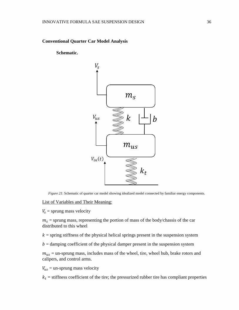
Schematic.
Figure 21: Schematic of quarter car model showing idealized model connected by familiar energy components.
List of Variables and Their Meaning:
𝑉𝑠 = sprung mass velocity
𝑚𝑠 = sprung mass, representing the portion of mass of the body/chassis of the car
distributed to this wheel
𝑘 = spring stiffness of the physical helical springs present in the suspension system
𝑏 = damping coefficient of the physical damper present in the suspension system
𝑚𝑢𝑠 = un-sprung mass, includes mass of the wheel, tire, wheel hub, brake rotors and
calipers, and control arms.
𝑉𝑢𝑠 = un-sprung mass velocity
𝑘𝑡 = stiffness coefficient of the tire; the pressurized rubber tire has compliant properties

INNOVATIVE FORMULA SAE SUSPENSION DESIGN 37
Bond Graph.
Figure 22: Fully augmented and numbered bond graph of quarter car model.
Derivation of state space equations and matrix. Given that the applied causality
to the bond graph of the simple quarter car model is all in integral form (the causal stroke
indicating that effort is flowing into the inertial elements and out of the capacitive
elements) the derivation of the system’s state equations is very straight forward. In this
system there exist 4 state variables, (𝑞2̇, 𝑝5̇, 𝑞8̇, 𝑝12̇ ) and 3 input variables,
(𝑉𝑖𝑛,𝑚𝑢𝑠𝑔,𝑚𝑠𝑔). It shall be noted that the primary input to this system is 𝑉𝑖𝑛 which
represents the change in velocity caused by the movement of the wheel against a variable
road surface which may have bumps, holes, drops, etc. The other input variables come
from an analysis including the effect of gravity on both the sprung and un-sprung masses
and are in fact not particularly necessary if the assumption is made that the springs in the

INNOVATIVE FORMULA SAE SUSPENSION DESIGN 38
system are already at their equilibrium position. However, for ease of intuition in this first
quarter car model, they will be kept in the analysis to avoid confusion as these effort
sources will be included in the analyses of the following half car models.
𝑞2̇ = 𝑉𝑖𝑛(𝑡) −𝑝5
𝑚𝑢𝑠 (3)
𝑝5̇ = 𝑞2𝑘𝑡 − 𝑚𝑢𝑠𝑔 − 𝑞8𝑘 − 𝑏 (𝑝5
𝑚𝑢𝑠−
𝑝12
𝑚𝑠) (4)
𝑞8̇ =𝑝5
𝑚𝑢𝑠−
𝑝12
𝑚𝑠 (5)
𝑝12̇ = 𝑞8𝑘 + 𝑏 (𝑝5
𝑚𝑢𝑠−
𝑝12
𝑚𝑠) − 𝑚𝑠𝑔 (6)
These state variable equations can then be put into state space matrix form, 𝑌 = [𝐴]�̅� +
[𝐵]�̅�, shown as follows:
[
𝑞2̇
𝑞8̇
𝑝5̇
𝑝12̇
] =
[ 0 0 −
1
𝑚𝑢𝑠0
0 01
𝑚𝑢𝑠−
1
𝑚𝑠
𝑘 −𝑘 −𝑏
𝑚𝑢𝑠
𝑏
𝑚𝑠
0 𝑘𝑏
𝑚𝑢𝑠−
𝑏
𝑚𝑠]
[
𝑞2
𝑞8
𝑝5
𝑝12
] + [
1 0 00 0 00 −1 00 0 1
] [𝑉𝑖𝑛
𝑚𝑢𝑠𝑔𝑚𝑠𝑔
] (7)
With the state space equations in matrix form, manipulation can be done to put
the system into the Laplace domain, to effectively solve the system of first order
differential equations by algebraic manipulation. This is done by operating on the A
matrix, subtracting each element from a 4x4 matrix made by multiplying the Laplacian
operator S by the identity matrix of equal size to the A matrix. Essentially, [𝐴] becomes
[𝑆𝐼 − 𝐴], and the rest of the system is put into the Laplace domain, shown by equation 8.

INNOVATIVE FORMULA SAE SUSPENSION DESIGN 39
[
𝑆𝑄2(𝑆)
𝑆𝑄8(𝑆)𝑆𝑃5(𝑆)
𝑆𝑃12(𝑆)
] =
[ 𝑆 0
1
𝑚𝑢𝑠
0
0 𝑆 −1
𝑚𝑢𝑠
1
𝑚𝑠
−𝑘 𝑘 𝑆 +𝑏
𝑚𝑢𝑠
−𝑏
𝑚𝑠
0 −𝑘 −𝑏
𝑚𝑢𝑠
𝑆 +𝑏
𝑚𝑠]
[
𝑞2(𝑆)
𝑞8(𝑆)𝑝5(𝑆)
𝑝12 (𝑆)
] + [
1 0 00 0 00 −1 00 0 1
] [
𝑉𝑖𝑛(𝑆)
𝑚𝑢𝑠𝑔(𝑆)
𝑚𝑠𝑔(𝑆)] (8)
From this point, various transfer functions may be found. A transfer function
relates a ratio of an output to an input of the system, to see how the behavior is affected.
The most insightful transfer function of the quarter car system is the relationship between
the velocity of the sprung mass of the vehicle and the input velocity as the wheel receives
bumps from the road. This relationship relates directly to driver comfort, making it a
desirable system behavior to know. The transfer function is solved by Cramer’s rule,
taking the quotient of two determinants. The numerator replaces the output variable
vector with the input variable vector before solving the determinants. In this case the
output variable is the velocity of the sprung mass, which may be solved with the state
variable of 𝑝12, the momentum of the sprung mass. It is known 𝑝 = 𝑚𝑉, so solving by
simple algebra the velocity may be found by 𝑉 =𝑝
𝑚.
𝑉𝑚𝑠
𝑉𝑖𝑛
(𝑆) =1
𝑚𝑠
∗
|
|
|
𝑆 01
𝑚𝑢𝑠1
0 𝑆 −1
𝑚𝑢𝑠0
−𝑘 𝑘 𝑆 +𝑏
𝑚𝑢𝑠0
0 −𝑘 −𝑏
𝑚𝑢𝑠0
|
|
|
|
|
|
𝑆 01
𝑚𝑢𝑠0
0 𝑆 −1
𝑚𝑢𝑠
1𝑚𝑠
−𝑘 𝑘 𝑆 +𝑏
𝑚𝑢𝑠−
𝑏𝑚𝑠
0 −𝑘 −𝑏
𝑚𝑢𝑠𝑆 +
𝑏𝑚𝑠
|
|
|
(9)

INNOVATIVE FORMULA SAE SUSPENSION DESIGN 40
𝑉𝑚𝑠
𝑉𝑖𝑛
(𝑆) =𝑘2 + 𝑆 𝑏 𝑘
(𝑚𝑢𝑠𝑆4 + 𝑏 𝑆3 + 2 𝑘 𝑆2)𝑚𝑠 + 𝑏 𝑚𝑢𝑠𝑆
3 + 𝑚𝑢𝑠𝑆2𝑘 + 𝑏 𝑆 𝑘 + 𝑘2
(10)
With a transfer function between the input velocity and the velocity of the sprung
mass, various analyses may be done on the system to see how it behaves with specific
given parameters. Results of such an analyses are demonstrated by Figure 23 with plots
for the amplitude ratio of the sprung mass to the input velocity and the phase angle
plotted along an increasing frequency. However, it is necessary first to list the values
assigned to the parameters in the equation to give context and meaning to the plots. These
are found in Table 2.
Table 2: Values assigned to parameters in quarter car equations used to create plots of frequency response behavior.
Parameter Value Units
𝑚𝑢𝑠 8.0 kg
𝑘 4000 Nm/deg
𝑘𝑡 123464 N/m
𝑚𝑠 182/4 *for 400lb vehicle kg
𝑏
0.6(2)𝑚𝑠√𝑘
𝑚𝑠
Ns/m
INNOVATIVE FORMULA SAE SUSPENSION DESIGN 41
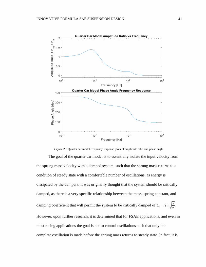
Figure 23: Quarter car model frequency response plots of amplitude ratio and phase angle.
The goal of the quarter car model is to essentially isolate the input velocity from
the sprung mass velocity with a damped system, such that the sprung mass returns to a
condition of steady state with a comfortable number of oscillations, as energy is
dissipated by the dampers. It was originally thought that the system should be critically
damped, as there is a very specific relationship between the mass, spring constant, and
damping coefficient that will permit the system to be critically damped of 𝑏𝑐 = 2𝑚√𝑘
𝑚 .
However, upon further research, it is determined that for FSAE applications, and even in
most racing applications the goal is not to control oscillations such that only one
complete oscillation is made before the sprung mass returns to steady state. In fact, it is

INNOVATIVE FORMULA SAE SUSPENSION DESIGN 42
more desired that the damping ratio 𝑏
𝑏𝑐 be somewhere around 0.5 to 0.7 for the best road
feel and vehicle control. With a damping ratio in this range, there is not such drastic
lateral load transfer in cornering, so the inside wheel on the turn is allowed to keep more
vertical load on it which helps to increase grip and overall cornering capacity. This was
taken into consideration when applying values to the MATLAB calculations for the plots
in this report. It shall be acknowledged that most performance dampers are designed to
have different damping coefficients in compression and rebound. However, for the
purposes of analysis one can simply consider multiple plots of various damping ratios
and evaluate the curves correspondingly.
Despite all this, the quarter car model is very well known as automotive
companies seek to outfit their vehicles with the best possible comfort to increase sales
and satisfaction. What is less well known, and has not been analyzed much before with
the bond graph approach is the relationship between the two lateral halves of the
vehicle’s suspension, meaning the right and left side of the car, as opposed to front to
back half. Longitudinal models have been studied to investigate the behaviors of dive and
squat. Lateral suspension behavior was investigated here in the conventional and
Koenigsegg half car models in the following sections.
Though the primary focus of this investigation is on lateral behavior in a half car
model, it is necessary to also introduce the effects of dive and squat, as a third damper
system serves to counteract the negative effects of these behaviors. Dive pulls the nose of
the car down when braking as load transfer due to negative acceleration (slowing down)
causes spring compression in the front end, requiring the front wheels to handle the
INNOVATIVE FORMULA SAE SUSPENSION DESIGN 43
majority of the braking power. This is never a beneficial quality; maximum braking
power is obtained when all four wheels are loaded equally. Squat pulls the rear of the car
down when accelerating, as load transfer due to positive acceleration (launch, or
increasing speed) causes additional spring compression in the rear. This is sometimes a
desired behavior as rear-wheel drive vehicles can transmit more power during launch
with a greater normal force.
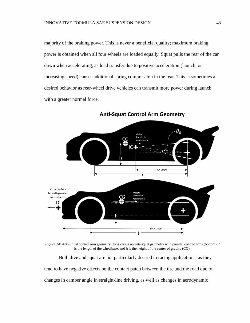
Figure 24: Anti-Squat control arm geometry (top) versus no anti-squat geometry with parallel control arms (bottom). 𝑙 is the length of the wheelbase, and h is the height of the center of gravity (CG).
Both dive and squat are not particularly desired in racing applications, as they
tend to have negative effects on the contact patch between the tire and the road due to
changes in camber angle in straight-line driving, as well as changes in aerodynamic

INNOVATIVE FORMULA SAE SUSPENSION DESIGN 44
influence and ride height. Changes in the orientation of the control arms can alter the
percent of anti-dive or anti-squat geometry the vehicle has, by putting longitudinal load
transfer more into tensile and compressive forces acting on the control arms and linkages
rather than entirely into the springs and dampers. Figure 24 helps to visualize the
suspension orientation changes made to counteract squat. The percentage of anti-squat
made by the angle of the control arms can be calculated as follows with reference to
Figure 24.
%𝐴𝑛𝑡𝑖 − 𝑆𝑞𝑢𝑎𝑡 =tan(𝜃𝑅)
ℎ𝑙
∗ 100 (11)
The top vehicle depicts anti-squat geometry of about 52%, assuming 𝜃𝑅 = 5𝑑𝑒𝑔,
ℎ = 11.0𝑖𝑛, and 𝑙 = 65.0𝑖𝑛. The bottom vehicle in the Figure demonstrates 0% anti-
squat with both control arms made parallel to the ground. This effectively puts the
instantaneous center (IC) infinitely far away so 𝜃𝑅 goes to zero, and the numerator of
equation 11 is then zero.
However, though it is beneficial to distribute some of the load out of the springs
to reduce spring compression and therefore total squat/dive, the distribution of these
loads demand that the control arms be made stronger to withstand greater stresses.
Assuming the same material is used for the control arms, greater strength requires more
material, resulting in more un-sprung mass.
Everything not directly contained by the chassis is considered “sprung mass,”
(because it is suspended by the springs). Everything else, including the wheels, tires,
wheel hubs, brake rotors, calipers, and control arms are considered “un-sprung mass.” It

INNOVATIVE FORMULA SAE SUSPENSION DESIGN 45
is imperative for the benefits of a vehicle’s frequency response and overall dynamics to
have the least possible un-sprung mass; this means there is less inertia and momentum
related to wheel movements with irregularities of the road surface, resulting in less
influence of residual motion into the sprung mass. When the control arms are forced to be
more massive to handle increased stresses by directing squat and dive forces into them, it
increases the un-sprung mass and makes the system more difficult to control.
A third damper system serves to minimize the magnitude of squat and dive
experienced during longitudinal load transfer by dissipating some of this energy into the
hydraulic fluid of the damper. When two wheels both move up at the same time very
rapidly (as in the case of hard braking from high speed) and a damper is connected
transversely between them, it is compressed from both sides. This movement forces the
piston to move rapidly within its hydraulic fluid, transferring energy into heat that would
otherwise go into compression or extension of the springs.
Conventional Transverse Half Car Model Analysis
The transverse half car model investigates the concepts of what happens to body
roll when a single wheel experiences a velocity change input. Traditionally, a component
known as the “sway bar” or “anti-roll bar” is installed that connects two wheels
transversely by way of a U-shaped bar that elastically deforms in torsion to act as a
spring. This is done such that when the body experiences roll, and the outer wheels travel
up as their springs and dampers compress, it will cause torsion on the sway bar that will
also pull up on the other wheel, effectively working to help balance out the effects of roll
in a turn to maintain the best contact patch possible between the tires and the road.
INNOVATIVE FORMULA SAE SUSPENSION DESIGN 46
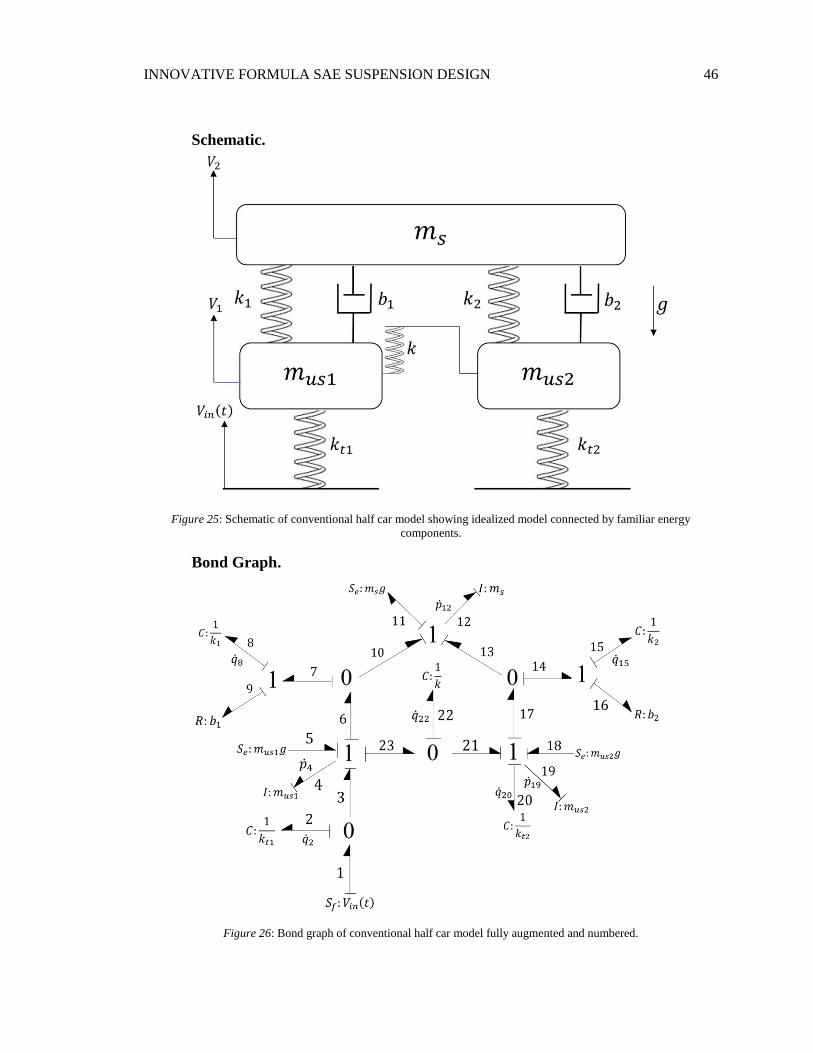
Schematic.
Figure 25: Schematic of conventional half car model showing idealized model connected by familiar energy
components.
Bond Graph.
Figure 26: Bond graph of conventional half car model fully augmented and numbered.

INNOVATIVE FORMULA SAE SUSPENSION DESIGN 47
Derivation of state space equations and matrix. The following 8 equations list
the final equations derived from following the analysis of the bond graph given the
assigned augmentation with compression considered positive. The hand calculations for
these equations may be found in Appendix D.
𝑞2̇ = 𝑉𝑖𝑛(𝑡) −𝑝4
𝑚𝑢𝑠1
(12)
𝑞8̇ =𝑝4
𝑚𝑢𝑠1
−𝑝12
𝑚𝑠
(13)
𝑞15̇ =𝑝19
𝑚𝑢𝑠2
−𝑝12
𝑚𝑠
(14)
𝑞20̇ =𝑝19
𝑚𝑢𝑠2
(15)
𝑞22̇ =𝑝4
𝑚𝑢𝑠1
−𝑝19
𝑚𝑢𝑠2
(16)
𝑝4̇ = 𝑞2𝑘𝑡1 + 𝑚𝑢𝑠1𝑔 − 𝑞8𝑘1 − 𝑏1 (𝑝4
𝑚𝑢𝑠1
−𝑝12
𝑚𝑠
) − 𝑞22𝑘 (17)
𝑝12̇ = −𝑚𝑠𝑔 + 𝑞8𝑘1 + 𝑏1 (𝑝4
𝑚𝑢𝑠1
−𝑝12
𝑚𝑠
) + 𝑞15𝑘2 + 𝑏2 (𝑝19
𝑚𝑢𝑠2
−𝑝12
𝑚𝑠
) (18)
𝑝19̇ = 𝑞22𝑘 + 𝑚𝑢𝑠2𝑔 − 𝑞15𝑘2 − 𝑏2 (𝑝19
𝑚𝑢𝑠2
−𝑝12
𝑚𝑠
) − 𝑞20𝑘𝑡2 (19)
To work with these equations requires that they be put into state-space matrix form. They
are listed in the order that they are to be arranged in the matrix shown by equation 20.
[ 𝑞2̇
𝑞8̇
𝑞15̇𝑞20̇𝑞22̇𝑝4̇
𝑝12̇𝑝19̇ ]
=
[ 0 0 0 0 0 −
1
𝑚𝑢𝑠10 0
0 0 0 0 01
𝑚𝑢𝑠1−
1
𝑚𝑠−
1
𝑚𝑠
0 0 0 0 0 0 −1
𝑚𝑠
1
𝑚𝑢𝑠2
0 0 0 0 0 0 01
𝑚𝑢𝑠2
0 0 0 0 01
𝑚𝑢𝑠10 −
1
𝑚𝑢𝑠2
𝑘𝑡1 −𝑘1 0 0 −𝑘 −𝑏1
𝑚𝑢𝑠1
𝑏1
𝑚𝑠0
0 𝑘1 𝑘2 0 0𝑏1
𝑚𝑢𝑠1(−
𝑏1 − 𝑏2
𝑚𝑠)
𝑏2
𝑚𝑢𝑠2
0 0 −𝑘2 −𝑘𝑡2 𝑘 0𝑏2
𝑚𝑠−
𝑏2
𝑚𝑢𝑠2]
[ 𝑞2
𝑞8
𝑞15
𝑞20
𝑞22
𝑝4
𝑝12
𝑝19]
+
[ 1 0 0 00 0 0 00 0 0 00 0 0 00 0 0 00 1 0 00 0 0 −10 0 1 0 ]
[
𝑉𝑖𝑛
𝑚𝑢𝑠1𝑔𝑚𝑢𝑠2𝑔𝑚𝑠𝑔
] (20)

INNOVATIVE FORMULA SAE SUSPENSION DESIGN 48
Though this matrix in equation 20 is substantially larger than the example demonstrated
by the quarter car model, the method of analysis is the same. We then converted to the
Laplacian domain, so [𝐴] becomes [𝑆𝐼 − 𝐴].
[ 𝑆𝑄2(𝑆)𝑆𝑄8(𝑆)
𝑆𝑄15(𝑆)𝑆𝑄20(𝑆)𝑆𝑄22(𝑆)𝑆𝑃4(𝑆)𝑆𝑃12(𝑆)
𝑆𝑃19(𝑆) ]
=
[ 𝑆 0 0 0 0
1
𝑚𝑢𝑠10 0
0 𝑆 0 0 0 −1
𝑚𝑢𝑠1
1
𝑚𝑠
1
𝑚𝑠
0 0 𝑆 0 0 01
𝑚𝑠−
1
𝑚𝑢𝑠2
0 0 0 𝑆 0 0 0 −1
𝑚𝑢𝑠2
0 0 0 0 𝑆 𝑆 −1
𝑚𝑢𝑠10
1
𝑚𝑢𝑠2
−𝑘𝑡1 𝑘1 0 0 𝑘𝑏1
𝑚𝑢𝑠1𝑆 −
𝑏1
𝑚𝑠0
0 −𝑘1 −𝑘2 0 0 −𝑏1
𝑚𝑢𝑠1𝑆 + (
𝑏1 − 𝑏2
𝑚𝑠) −
𝑏2
𝑚𝑢𝑠2
0 0 𝑘2 𝑘𝑡2 −𝑘 0 −𝑏2
𝑚𝑠𝑆 +
𝑏2
𝑚𝑢𝑠2]
[ 𝑄2(𝑆)𝑄8(𝑆)
𝑄15(𝑆)𝑄20(𝑆)𝑄22(𝑆)𝑃4(𝑆)𝑃12(𝑆)
𝑃19(𝑆) ]
+
[ 1 0 0 00 0 0 00 0 0 00 0 0 00 0 0 00 1 0 00 0 0 −10 0 1 0 ]
[
𝑉𝑖𝑛(𝑆)𝑚𝑢𝑠1𝑔(𝑆)𝑚𝑢𝑠2𝑔(𝑆)𝑚𝑠𝑔(𝑆)
] (21)
From this point, the transfer functions of interest may be derived. The interest
here was in determining the relationships between the input velocity and each wheel in
the system, as one wheel is directly affected by the input velocity to its tire, while the
other feels the input velocity only as it relates through the sprung mass and anti-roll bar.
This way, we can viably compare the behavior of each wheel responding to the same
input, with the only difference being the addition of the third damper. Therefore, I will
derive the transfer functions of 𝑉𝑚𝑢𝑠1
𝑉𝑖𝑛(𝑆) and
𝑉𝑚𝑢𝑠2
𝑉𝑖𝑛(𝑆), utilizing the Cramer’s rule
replacement and knowing fundamentally momentum is equal to mass times volume (𝑝 =
𝑚𝑉) as demonstrated by the quarter car model example.
The first of these transfer functions was set up as shown in equation 22, however
for conservation of space the writing out of this step for subsequent transfer functions
was omitted, skipping directly to the result of the quotient of the determinants stated by

INNOVATIVE FORMULA SAE SUSPENSION DESIGN 49
Cramer’s rule. However, it shall be noticed in this instance that the 6th column of the
matrix in the numerator corresponding to the momentum of 𝑚𝑢𝑠1 is replaced by the
vector corresponding to the input variable 𝑉𝑖𝑛 as dictated by the method of Cramer’s rule.
Then the quotient was divided by 1
𝑚𝑢𝑠1 to effectively convert the momentum of the first
un-sprung mass to its velocity to match the need of the transfer function.
𝑇𝐹1 =𝑉𝑚𝑢𝑠1
𝑉𝑖𝑛
(𝑆) =1
𝑚𝑢𝑠1∗
|
|
|
|
𝑆 0 0 0 0 1 0 0
0 𝑆 0 0 0 01𝑚𝑠
1𝑚𝑠
0 0 𝑆 0 0 01𝑚𝑠
−1
𝑚𝑢𝑠2
0 0 0 𝑆 0 0 0 −1
𝑚𝑢𝑠2
0 0 0 0 𝑆 0 01
𝑚𝑢𝑠2
−𝑘𝑡1 𝑘1 0 0 𝑘 0 𝑆 −𝑏1𝑚𝑠
0
0 −𝑘1 −𝑘2 0 0 0 𝑆 + (𝑏1 − 𝑏2
𝑚𝑠) −
𝑏2𝑚𝑢𝑠2
0 0 𝑘2 𝑘𝑡2 −𝑘 0 −𝑏2𝑚𝑠
𝑆 +𝑏2
𝑚𝑢𝑠2
|
|
|
|
|
|
|
|
|
𝑆 0 0 0 01
𝑚𝑢𝑠10 0
0 𝑆 0 0 0 −1
𝑚𝑢𝑠1
1𝑚𝑠
1𝑚𝑠
0 0 𝑆 0 0 01𝑚𝑠
−1
𝑚𝑢𝑠2
0 0 0 𝑆 0 0 0 −1
𝑚𝑢𝑠2
0 0 0 0 𝑆 𝑆 −1
𝑚𝑢𝑠10
1𝑚𝑢𝑠2
−𝑘𝑡1 𝑘1 0 0 𝑘𝑏1
𝑚𝑢𝑠1𝑆 −
𝑏1𝑚𝑠
0
0 −𝑘1 −𝑘2 0 0 −𝑏1
𝑚𝑢𝑠1𝑆 + (
𝑏1 − 𝑏2𝑚𝑠
) −𝑏2
𝑚𝑢𝑠2
0 0 𝑘2 𝑘𝑡2 −𝑘 0 −𝑏2𝑚𝑠
𝑆 +𝑏2
𝑚𝑢𝑠2
|
|
|
|
|
(22)
This equation was solved in MATLAB as it would be extremely tedious and
impractical to solve by hand. The code for this and the following determinant calculations
may be found in Appendix C. The result even simplified is very lengthy, and will be
separated into numerator and denominator portions for clarity.
(23)

INNOVATIVE FORMULA SAE SUSPENSION DESIGN 50
𝑇𝐹1𝑁𝑈𝑀 = ((𝑆3𝑏2𝑘𝑡1 + 𝑆2𝑘 𝑘𝑡1 + 𝑆2𝑘2𝑘𝑡1 + 𝑆2𝑘𝑡1𝑘𝑡2 + 𝑆4𝑘𝑡1𝑚𝑢𝑠2)𝑚𝑠2
+ (𝑘 𝑘1𝑘𝑡1 − 2 𝑆2𝑏22𝑘𝑡1 + 𝑘 𝑘2𝑘𝑡1 + 𝑘1𝑘2𝑘𝑡1 + 𝑘1𝑘𝑡1𝑘𝑡2 + 𝑘2𝑘𝑡1𝑘𝑡2
+ 𝑆2𝑏1𝑏2𝑘𝑡1 + 𝑆3𝑏1𝑘𝑡1𝑚𝑢𝑠2 − 𝑆3𝑏2𝑘𝑡1𝑚𝑢𝑠2 + 𝑆2𝑘1𝑘𝑡1𝑚𝑢𝑠2 + 𝑆2𝑘2𝑘𝑡1𝑚𝑢𝑠2
+ 𝑆 𝑏1𝑘 𝑘𝑡1 − 𝑆 𝑏2𝑘 𝑘𝑡1 + 𝑆 𝑏1𝑘2𝑘𝑡1 + 𝑆 𝑏2𝑘1𝑘𝑡1 − 2 𝑆 𝑏2𝑘2𝑘𝑡1 + 𝑆 𝑏1𝑘𝑡1𝑘𝑡2
− 𝑆 𝑏2𝑘𝑡1𝑘𝑡2)𝑚𝑠 + 𝑘1𝑘2𝑘𝑡1𝑚𝑢𝑠2 + 𝑆 𝑏2𝑘1𝑘𝑡1𝑚𝑢𝑠2)
𝑇𝐹1𝐷𝐸𝑁𝑂𝑀 = ((𝑆4𝑏1𝑏2 + 𝑆3𝑏1𝑘 + 𝑆3𝑏2𝑘 + 𝑆3𝑏1𝑘2 + 𝑆3𝑏2𝑘1 + 𝑆3𝑏1𝑘𝑡2 + 𝑆3𝑏2𝑘𝑡1
+ 𝑆5𝑏1𝑚𝑢𝑠2 + 𝑆5𝑏2𝑚𝑢𝑠1 + 𝑆2𝑘 𝑘1 + 𝑆2𝑘 𝑘2 + 𝑆2𝑘 𝑘𝑡1 + 𝑆2𝑘 𝑘𝑡2 + 𝑆2𝑘1𝑘2
+ 𝑆2𝑘1𝑘𝑡2 + 𝑆2𝑘2𝑘𝑡1 + 𝑆2𝑘𝑡1𝑘𝑡2 + 𝑆4𝑘 𝑚𝑢𝑠1 + 𝑆4𝑘 𝑚𝑢𝑠2 + 𝑆4𝑘1𝑚𝑢𝑠2
+ 𝑆4𝑘2𝑚𝑢𝑠1 + 𝑆4𝑘𝑡1𝑚𝑢𝑠2 + 𝑆4𝑘𝑡2𝑚𝑢𝑠1 + 𝑆6𝑚𝑢𝑠1𝑚𝑢𝑠2)𝑚𝑠2
+ (𝑘 𝑘1𝑘𝑡1 − 2 𝑆2𝑏22𝑘 − 2 𝑆2𝑏2
2𝑘1 − 2 𝑆2𝑏22𝑘𝑡1 − 2 𝑆4𝑏2
2𝑚𝑢𝑠1 − 2 𝑆3𝑏1𝑏22
+ 𝑘 𝑘1𝑘𝑡2 + 𝑘 𝑘2𝑘𝑡1 + 𝑘 𝑘2𝑘𝑡2 + 𝑘1𝑘2𝑘𝑡1 + 𝑘1𝑘2𝑘𝑡2 + 𝑘1𝑘𝑡1𝑘𝑡2 + 𝑘2𝑘𝑡1𝑘𝑡2
− 2 𝑆2𝑏1𝑏2𝑘 − 2 𝑆2𝑏1𝑏2𝑘2 + 𝑆2𝑏1𝑏2𝑘𝑡1 − 𝑆2𝑏1𝑏2𝑘𝑡2 + 𝑆4𝑏1𝑏2𝑚𝑢𝑠1
− 𝑆4𝑏1𝑏2𝑚𝑢𝑠2 + 𝑆3𝑏1𝑘 𝑚𝑢𝑠1 + 𝑆3𝑏1𝑘 𝑚𝑢𝑠2 − 𝑆3𝑏2𝑘 𝑚𝑢𝑠1 − 𝑆3𝑏2𝑘 𝑚𝑢𝑠2
+ 𝑆3𝑏1𝑘2𝑚𝑢𝑠1 + 𝑆3𝑏2𝑘1𝑚𝑢𝑠1 + 𝑆3𝑏1𝑘2𝑚𝑢𝑠2 − 𝑆3𝑏2𝑘1𝑚𝑢𝑠2 − 2 𝑆3𝑏2𝑘2𝑚𝑢𝑠1
+ 𝑆3𝑏1𝑘𝑡1𝑚𝑢𝑠2 + 𝑆3𝑏1𝑘𝑡2𝑚𝑢𝑠1 − 𝑆3𝑏2𝑘𝑡1𝑚𝑢𝑠2 − 𝑆3𝑏2𝑘𝑡2𝑚𝑢𝑠1
+ 𝑆5𝑏1𝑚𝑢𝑠1𝑚𝑢𝑠2 − 𝑆5𝑏2𝑚𝑢𝑠1𝑚𝑢𝑠2 + 𝑆2𝑘 𝑘1𝑚𝑢𝑠1 + 𝑆2𝑘 𝑘2𝑚𝑢𝑠1
+ 𝑆2𝑘 𝑘2𝑚𝑢𝑠2 + 𝑆2𝑘1𝑘2𝑚𝑢𝑠1 + 𝑆2𝑘1𝑘2𝑚𝑢𝑠2 + 𝑆2𝑘1𝑘𝑡1𝑚𝑢𝑠2 + 𝑆2𝑘1𝑘𝑡2𝑚𝑢𝑠1
+ 𝑆2𝑘2𝑘𝑡1𝑚𝑢𝑠2 + 𝑆2𝑘2𝑘𝑡2𝑚𝑢𝑠1 + 𝑆4𝑘1𝑚𝑢𝑠1𝑚𝑢𝑠2 + 𝑆4𝑘2𝑚𝑢𝑠1𝑚𝑢𝑠2
− 2 𝑆 𝑏2𝑘 𝑘1 − 2 𝑆 𝑏2𝑘 𝑘2 + 𝑆 𝑏1𝑘 𝑘𝑡1 + 𝑆 𝑏1𝑘 𝑘𝑡2 − 𝑆 𝑏2𝑘 𝑘𝑡1 − 𝑆 𝑏2𝑘 𝑘𝑡2
− 2 𝑆 𝑏2𝑘1𝑘2 + 𝑆 𝑏1𝑘2𝑘𝑡1 + 𝑆 𝑏2𝑘1𝑘𝑡1 + 𝑆 𝑏1𝑘2𝑘𝑡2 − 𝑆 𝑏2𝑘1𝑘𝑡2 − 2 𝑆 𝑏2𝑘2𝑘𝑡1
+ 𝑆 𝑏1𝑘𝑡1𝑘𝑡2 − 𝑆 𝑏2𝑘𝑡1𝑘𝑡2)𝑚𝑠 + 𝑘1𝑘2𝑘𝑡1𝑚𝑢𝑠2 + 2 𝑆 𝑏2𝑘 𝑘1𝑚𝑢𝑠2
+ 𝑆 𝑏2𝑘1𝑘𝑡1𝑚𝑢𝑠2 + 𝑆3𝑏2𝑘1𝑚𝑢𝑠1𝑚𝑢𝑠2 + 𝑆2𝑘1𝑘2𝑚𝑢𝑠1𝑚𝑢𝑠2)
It is evident that this system is of great complexity with a matrix of 8 state
variables, so the following mathematical results will not be displayed within the body of
this report, but rather will be handled internally within MATLAB, only plotting the
insightful behavioral results from a frequency response analysis on this system. The next
step in the analysis is to replace the Laplacian operator 𝑆 with 𝑗𝜔 to simulate a harmonic

INNOVATIVE FORMULA SAE SUSPENSION DESIGN 51
input, ultimately permitting an analysis of the frequency response and amplitude ratio of
the system. There exists a convenient function within MATLAB that can take the
coefficients of the S values of a transfer function system to plot both the frequency
response and phase angle, but given the length and complexity of this system, it is easier
to make these calculations “by hand” within the MATLAB code as reflected in Appendix
C, rather than manually searching through to find the coefficients of each degree of S.
Once these calculations are made, plots are created according to Figure 27. For relevance
of these plots, they were made with parameter values according to Table 3.
Table 3: Values assigned to parameters in half car equations used to create plots of frequency response behavior.
Parameter Value Units
𝑚𝑠 200 kg
𝑚𝑢𝑠1 8.0 kg
𝑚𝑢𝑠2 8.0 kg
𝑘1 4000 N/m
𝑘2 4000 N/m
𝑘 50000 Nm/deg
𝑘𝑡1 123464 N/m
𝑘𝑡2 123464 N/m
𝑚𝑠 182/4 *for 400lb vehicle kg
𝑏1 0.6(2)𝑚𝑠
4 √𝑘1
(𝑚𝑠
4 )
Ns/m
𝑏2 0.6(2)𝑚𝑠
4 √𝑘1
(𝑚𝑠
4 )
Ns/m

INNOVATIVE FORMULA SAE SUSPENSION DESIGN 52
Figure 27: Frequency response plots of the left un-sprung mass velocity to the input velocity in the conventional half-
car model.
By a similar process to equation 22, the transfer functions for 𝑉𝑚𝑠
𝑉𝑖𝑛(𝑆) and
𝑉𝑚𝑢𝑠2
𝑉𝑖𝑛(𝑆) were
calculated, converted to a harmonic input for frequency response analysis, and the
amplitude ratio and phase angles were plotted and calculated. The resulting plots of these
calculations are given below.

INNOVATIVE FORMULA SAE SUSPENSION DESIGN 53
Figure 28: Frequency response plots of the right un-sprung mass velocity to the input velocity in the conventional half-
car model.
Figure 29: Frequency response plots of the sprung mass velocity to the input velocity in the conventional half-car
model.

INNOVATIVE FORMULA SAE SUSPENSION DESIGN 54
Now for the most important plot of this conventional model, is to overlay the
frequency response amplitude ratio between the left and right un-sprung masses. This
will clearly show the difference between the behavior of the two wheels on either side of
the car when only one wheel experiences a bump or change in velocity while the other
continues on flat ground, but is forced to move because of the sway bar connection
between the two wheels.
Figure 30: Visual comparison of behavior between left and right wheels only connected by the sway bar.
Introduction to Koenigsegg Design
Christian von Koenigsegg, a Swedish hypercar manufacturer sought to innovate at
every opportunity possible. One of these brilliant innovations is his famous Triplex
suspension, which utilizes the addition of a third damper mounted transversely between
the two upper wishbone control arms of wheels on either side of the car. With this
addition and many others, he has successfully made some of the uncontested best racing
performance vehicles ever manufactured, winning all sorts of records and firsts.

INNOVATIVE FORMULA SAE SUSPENSION DESIGN 55
Koenigsegg Design Transverse Half-Car Model Analysis
Schematic.
Figure 31: Schematic of innovative half car model showing idealized model connected by familiar energy components.
Bond Graph.
Figure 32: Bond graph of innovative half car model fully augmented and numbered.

INNOVATIVE FORMULA SAE SUSPENSION DESIGN 56
Derivation of state space equations and matrix. The derivation of the state
space equations was quite similar to those derived for the conventional transverse half car
model being that the bond graphs are so similar and maintain integral causality. Very
conveniently, the derivations of all of the �̇� equations were exactly the same, so I will
refer you back to the previous section’s derivations for those expressed equations.
However, all three of the �̇� equations are slightly different with the addition of the third
damper to the system. This is intuitively expected, given that additional damping
naturally changes the momenta of masses within a system when acted upon by an input
velocity. These new equations are derived as follows:
𝑝4̇ = 𝑞2(𝑘𝑡1) + 𝑞8(−𝑘1) + 𝑞22(−𝑘) + 𝑝4 (−𝑏1 − 𝑏
𝑚𝑢𝑠1
) + 𝑝12 (𝑏1
𝑚𝑠
) + 𝑝19 (−𝑏
𝑚𝑢𝑠2
) + 𝑚𝑢𝑠1𝑔 (24)
𝑝12̇ = 𝑞8(𝑘1) + 𝑞15(𝑘2) + 𝑝4 (𝑏1
𝑚𝑢𝑠1
) + 𝑝12 (−𝑏1 − 𝑏2
𝑚𝑠
) + 𝑝19 (𝑏2
𝑚𝑢𝑠2
) − 𝑚𝑠𝑔 (25)
𝑝19̇ = 𝑞15(−𝑘2) + 𝑞20(−𝑘𝑡2) + 𝑞22(𝑘) + 𝑝4 (−𝑏
𝑚𝑢𝑠1
) + 𝑝12 (𝑏2
𝑚𝑠
) + 𝑝19 (−𝑏 − 𝑏2
𝑚𝑢𝑠2
) + 𝑚𝑢𝑠2𝑔 (26)
Since these state variable equations are new, the [𝐴] matrix of the state space matrix
equation was re-created, as shown with the vector replacements from equations 24 - 26.
[ 𝑞2̇
𝑞8̇
𝑞15̇𝑞20̇𝑞22̇𝑝4̇
𝑝12̇𝑝19̇ ]
=
[ 0 0 0 0 0 −
1
𝑚𝑢𝑠10 0
0 0 0 0 01
𝑚𝑢𝑠1−
1
𝑚𝑠−
1
𝑚𝑠
0 0 0 0 0 0 −1
𝑚𝑠
1
𝑚𝑢𝑠2
0 0 0 0 0 0 01
𝑚𝑢𝑠2
0 0 0 0 01
𝑚𝑢𝑠10 −
1
𝑚𝑢𝑠2
𝑘𝑡1 −𝑘1 0 0 −𝑘−𝑏1 − 𝑏
𝑚𝑢𝑠1
𝑏1
𝑚𝑠−
𝑏
𝑚𝑢𝑠2
0 𝑘1 𝑘2 0 0𝑏1
𝑚𝑢𝑠1(−𝑏1 − 𝑏2
𝑚𝑠)
𝑏2
𝑚𝑢𝑠2
0 0 −𝑘2 −𝑘𝑡2 𝑘 −𝑏
𝑚𝑢𝑠1
𝑏2
𝑚𝑠
−𝑏 − 𝑏2
𝑚𝑢𝑠2 ]
[ 𝑞2
𝑞8
𝑞15
𝑞20
𝑞22
𝑝4
𝑝12
𝑝19]
+
[ 1 0 0 00 0 0 00 0 0 00 0 0 00 0 0 00 1 0 00 0 0 −10 0 1 0 ]
[
𝑉𝑖𝑛
𝑚𝑢𝑠1𝑔𝑚𝑢𝑠2𝑔𝑚𝑠𝑔
] (27)

INNOVATIVE FORMULA SAE SUSPENSION DESIGN 57
If one were to compare the two A matrices, it is apparent that the only differences
appear in the 9 entries of the lower right corner of the matrix, corresponding to the
momentum variables. From this point, the same mathematical process as was done in the
conventional half car analysis was carried out. The plots of the behavior of the system
based on the same three transfer functions as derived previously, are shown in Figure 33
through Figure 36. For plot relevance, the values assigned to the equation parameters are
given in Table 4.
Table 4: Values assigned to parameters in Koenigsegg equations used to create plots of frequency response behavior.
Parameter Value Units
𝑚𝑠 200 kg
𝑚𝑢𝑠1 8.0 kg
𝑚𝑢𝑠2 8.0 kg
𝑘1 4000 N/m
𝑘2 4000 N/m
𝑘 50000 Nm/deg
𝑘𝑡1 123464 N/m
𝑘𝑡2 123464 N/m
𝑚𝑠 182/4 *for 400lb vehicle kg
𝑏1 0.6(2)𝑚𝑠
4 √𝑘1
(𝑚𝑠
4 )
Ns/m
𝑏2 0.6(2)𝑚𝑠
4 √𝑘1
(𝑚𝑠
4 )
Ns/m
𝑏 ( 𝑣𝑎𝑟𝑖𝑎𝑏𝑙𝑒 𝑐𝑜𝑒𝑓𝑓. ) ∗ 𝑏1 Ns/m

INNOVATIVE FORMULA SAE SUSPENSION DESIGN 58
Figure 33: Frequency response plots of the left un-sprung mass velocity to the input velocity in the transverse damper
half-car model.
Figure 34: Frequency response plots of the right un-sprung mass velocity to the input velocity in the transverse damper
half-car model.

INNOVATIVE FORMULA SAE SUSPENSION DESIGN 59
Figure 35: Frequency response plots of the sprung mass velocity to the input velocity in the transverse damper half-car
model.
Figure 36: Visual comparison of behavior between left and right wheels only connected by the sway bar and transverse
damper.

INNOVATIVE FORMULA SAE SUSPENSION DESIGN 60
Discussion
At long last, the final plot that is meant to truly tell the difference between the
effectiveness of a system with a transversely mounted third damper compared to one
without.
Figure 37: Comparison of right wheel response with and without transverse damper.
Through a grueling process, we have arrived at a visual plot that represents the
amplitude ratios of the right un-sprung masses of the two compared systems, and it is
clear that there is a winner among the two. Both of these systems were given the same
values for all the parameters, (spring stiffness, tire stiffness, damping coefficients, etc.)
aside from the obvious additional third damper which was an added parameter to the
transverse damper half car model. However, it is clear that the system with the added
transversely mounted damper caused the right wheel (the wheel that rides along flat

INNOVATIVE FORMULA SAE SUSPENSION DESIGN 61
ground) to have a significantly lesser amplitude ratio in relation to the input velocity
acting on the left side of the vehicle. Ultimately, this means that the contact patch and
contact forces between the right tire and the road are less affected, so power transmission
and grip are more steady, permitting greater tangential force from the ground and a faster
race car.
It is imperative to note that the values assigned to the parameters in this system by
no means represent an optimally tuned vehicle. The values assigned were found from
FSAE forums and online sources according to what teams have used in the past to get
reasonably good results. This means that there is a great deal of tuning to be done to
actually get the frequency response to something that will benefit the driving experience,
rather than accidentally cause resonance between masses that can go out of control very
quickly for a given input frequency. However, for a primitive approach to the suspension
design of a vehicle, in considering whether or not to make an addition of a third,
transversely mounted damper, it appears that it would provide a great benefit to the
vehicle’s power transmission to the ground by having a lesser effect on wheels traveling
on flat ground that are pulled up by the anti-roll bar torsion.
Semi-Active System Control with Magnetorheological Dampers
There exist three types of suspension system control: passive, semi-active, and
active. In passive systems, the energy parameters of the system (spring stiffness and
damping coefficient) are set to static values. This only allows the suspension setup to be
effective over a specific frequency range. However, if the system and its operating
conditions are changed, the optimum performance cannot be achieved. Active control

INNOVATIVE FORMULA SAE SUSPENSION DESIGN 62
systems however impart a force or velocity on the system to directly counteract specific
behaviors over a very wide range of frequencies, but generally require a large power
supply or are heavy and are therefore not ideal for racing situations. Semi-active control
changes the vehicle parameters to change the behavioral response of the system without
imparting an additional force from an outside energy source. This type of control is
highly appealing with its low-mass implementation and no need for additional energy
inputs, with applications over a much wider frequency range than passive suspension.
With the rise in automotive electronics and sensor monitoring contributing to
computational control of vehicle dynamics parameters, the opportunities for suspension
control are increased greatly. Magnetorheological (MR) damper technology hit the
commercial market in about 2004, developed by the General Motors Delphi Automotive
Division. The opportunities of this semi-active control mechanism were limited at first
due to a lack of understanding and controllability. However, further iterations and newer
models coupled with more accurate sensors and faster reactive computing has led to an
innovative means of suspension design. Koenigsegg included these MR dampers into
their vehicles for a highly controllable system whose frequency response behavior can be
semi-actively controlled through both reactive and predictive settings of the MR dampers
to change the effective hydraulic fluid viscosity and alter the damping coefficient of the
damper.
Magnetorheological fluid is a fluid with iron particles in it that responds to a
magnetic stimulus, changing shape and/or viscosity. Engineers have implemented the use
of magnetorheological fluid within dampers by adding iron particles to hydraulic fluid,
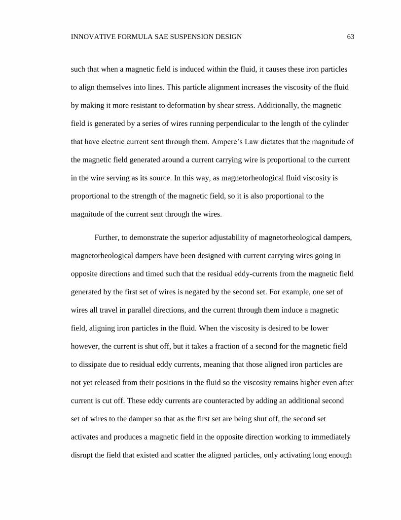
INNOVATIVE FORMULA SAE SUSPENSION DESIGN 63
such that when a magnetic field is induced within the fluid, it causes these iron particles
to align themselves into lines. This particle alignment increases the viscosity of the fluid
by making it more resistant to deformation by shear stress. Additionally, the magnetic
field is generated by a series of wires running perpendicular to the length of the cylinder
that have electric current sent through them. Ampere’s Law dictates that the magnitude of
the magnetic field generated around a current carrying wire is proportional to the current
in the wire serving as its source. In this way, as magnetorheological fluid viscosity is
proportional to the strength of the magnetic field, so it is also proportional to the
magnitude of the current sent through the wires.
Further, to demonstrate the superior adjustability of magnetorheological dampers,
magnetorheological dampers have been designed with current carrying wires going in
opposite directions and timed such that the residual eddy-currents from the magnetic field
generated by the first set of wires is negated by the second set. For example, one set of
wires all travel in parallel directions, and the current through them induce a magnetic
field, aligning iron particles in the fluid. When the viscosity is desired to be lower
however, the current is shut off, but it takes a fraction of a second for the magnetic field
to dissipate due to residual eddy currents, meaning that those aligned iron particles are
not yet released from their positions in the fluid so the viscosity remains higher even after
current is cut off. These eddy currents are counteracted by adding an additional second
set of wires to the damper so that as the first set are being shut off, the second set
activates and produces a magnetic field in the opposite direction working to immediately
disrupt the field that existed and scatter the aligned particles, only activating long enough

INNOVATIVE FORMULA SAE SUSPENSION DESIGN 64
to disrupt these residual eddy currents and then shutting off before realigning the particles
with the new magnetic field orientation.
However, the practical use of MR dampers is significantly hindered by its
characteristic hysteretic and non-linear dynamics. Such behavior makes the effective
damping coefficient and damping forces with a given velocity difficult to calculate and
predict. Therefore, for a successful implementation of MR dampers into a system, it
demands an accurate model of the damper, and an effective control strategy in how the
system calculates the current to be produced through the damper based on input variables.
There exist a few different models that are designed to help predict the dynamics of the
MR damper. These models include NARX, viscoelastic-plastic, nonlinear blackbox,
fuzzy, neural network developed by Chang and Roschke, phenomenological based on a
Bouc-Wen hysteresis model, and polynomial among others.
Figure 38: Right wheel frequency response plotted over a range of transverse damping coefficients. These coefficients
are given as ratios of the damping coefficient at each individual wheel (𝑏1) which has a damping ratio of 0.6, for
reference with respect to other vehicle parameters.

INNOVATIVE FORMULA SAE SUSPENSION DESIGN 65
Figure 39:Right wheel frequency response plotted over a range of transverse damping coefficients. The 𝑏1 damping
coefficient is given a damping ratio of 0.707 as opposed to 0.6 in Figure 38.
Figure 38 and 39 give great insight into the areas of control available with a
variable damping coefficient. Using an MR damper the frequency response of a system is
no longer limited to a single curve, but a whole range based on a variable damping
coefficient. If a successful model of the MR damper behavior is created such that the
effective damping coefficient is accurately related to an electrical input current, the
system could be coded to input a specific current based on sensor data to immediately set
a damping coefficient that will yield optimum control at the frequency observed. For
example, as the vehicle races around the track, the sensors will constantly be feeding data
into the onboard computer. The desired damping force can be calculated according to the
force and velocity of the input, and if the damper motion velocity is also measured by a
sensor, the input current can be calculated according to the model generated of the MR
damper behavior to yield the desired damping force.

INNOVATIVE FORMULA SAE SUSPENSION DESIGN 66
Conclusion
Though a suspension system is simple in principle, the design process is no small
feat – especially for racing applications where every fraction of a second counts. Further,
the analysis of suspension systems is arguably more complicated to yield helpful results
that may be interpreted allowing for improvement to the system as a whole. The dynamic
systems bond graph approach to this comparison of suspension designs makes for an easy
to follow process, but is sometimes not so easy to manipulate and interpret the results. In
the process of calculating the necessary determinants, transfer functions, amplitude ratios,
and phase angles necessary to plot frequency response of different aspects of the system,
at times the mathematics seemed overwhelming. Eight state variables results in an 8x8
linear system when converted to the Laplacian domain, such that when transfer functions
were calculated through MATLAB, the resulting equation put into a Word document was
well over a page in length. This goes to show the overall complexity of the systems being
analyzed, and the power of modern computation. Symbolic 8x8 determinants alone
would take dozens of hours to calculate, but when the matrices of the system are entered
correctly into MATLAB, they can be calculated in fractions of a second. There is much
work to be done as far as tuning the values assigned to the system parameters to yield
more desirable frequency response plots, which will be done in further work on the
subject outside of this report.
Ultimately, this investigation and comparison was a challenging process that
required the full application of Dynamic Systems Modeling to work through the analysis

INNOVATIVE FORMULA SAE SUSPENSION DESIGN 67
from start to finish. I am glad for the challenge and look forward to continuing this work
in the full design of the Liberty University FSAE suspension system.
Limitations and Future Work
This work could be improved by mathematical plots with input values and
parameters measured from a physical system for greater accuracy and meaningful results.
In my limited knowledge of suspension design, though I have learned a great deal to
reach the current design of this system, I have a great deal left to learn in optimizing each
aspect of force and movement that the suspension is responsible for. With this being
Liberty University’s first FSAE vehicle, I have no previous model to test and learn from,
only my textbooks and online resources.
Further investigation is planned to be done by empirical testing on the
manufactured Formula SAE vehicle with and without the transverse third damper
connected to the system to gather squat and dive curves, and best fit an effective quarter
car damping coefficient to simulate the anti-squat and anti-dive characteristics of a third
damper addition. Additionally, single-sided disturbances will be investigated in an effort
to gather vertical displacement data of the opposite wheel to validate the mathematical
model created by the dynamic systems analysis and plotted in MATLAB. Measured
coefficients from the vehicle such as mass, spring rate, damping coefficient etc. can be
gathered and input into the MATLAB program to establish the mathematical baseline
against which to compare empirical data plots.

INNOVATIVE FORMULA SAE SUSPENSION DESIGN 68
References
1. Koenigsegg. (2016, December 13). Build 7128 - Subframe and Suspension.
Retrieved from https://www.koenigsegg.com/build-7128-subframe-and-
suspension/
2. Carbibles. (2018, August 05). Complete Guide to Car Suspension. Retrieved from
https://www.carbibles.com/guide-to-car-suspension/
3. Sharp, R. S. (2002). Wheelbase filtering and automobile suspension tuning for
minimizing motions in pitch. Proceedings of the Institution of Mechanical
Engineers, Part D: Journal of Automobile Engineering,216(12), 933-946.
doi:10.1243/095440702762508182
4. R. S. SHARP, D. A. CROLLA. (1987) Road Vehicle Suspension System Design -
a review. Vehicle System Dynamics 16:3, pages 167-192.
5. TORE DAHLBERG. (1980) Comparison of Ride Comfort Criteria for Computer
Optimization of Vehicles Travelling on Randomly Profiled Roads. Vehicle System
Dynamics 9:6, pages 291-307.
6. D. RYBA. (1974) Improvement in Dynamic Characteristics of Automobile
Suspension Systems Part II - Three-Mass System. Vehicle System Dynamics 3:2,
pages 55-98.
7. R S Sharp, S A Hassan. (1986) The Relative Performance Capabilities of Passive,
Active and Semi-Active Car Suspension Systems. Proceedings of the Institution
of Mechanical Engineers, Part D: Transport Engineering 200:3, pages 219-228.
8. D A Crolla, D N L Horton, R H Pitcher, J A Lines. (1987) Active Suspension
Control for an Off-Road Vehicle. Proceedings of the Institution of Mechanical
Engineers, Part D: Transport Engineering 201:1, pages 1-10.
9. A H Kalyan Raj, C Padmanabhan. (2009) A new passive non-linear damper for
automobiles. Proceedings of the Institution of Mechanical Engineers, Part D:
Journal of Automobile Engineering 223:11, pages 1435-1443.

INNOVATIVE FORMULA SAE SUSPENSION DESIGN 69
10. Furukawa, A., & Ishikawa, M. (1981). Outline of Ultra Light Weight Vehicle and
Its Body Design. SAE Technical Paper Series. doi:10.4271/811381
11. Santos, Rodrigo de Oliveira. “Racing Car Dynamics - Your Technical Blog on
Race Cars.” Racing Car Dynamics - Your Uncomplicated Resource to Race
Engineering, Rodrigo Santos, 29 Oct. 2015, racingcardynamics.com/.
12. Gillespie, T. D. Fundamentals of Vehicle Dynamics: a Professional Development
Technical Video Tutorial Series: Workbook & Educational Support Material.
Society of Automotive Engineers, 1995.
13. Pacejka, Hans B. Tyre and Vehicle Dynamics. Elsevier Butterworth-Heinemann,
2009.
14. Rajamani, Rajesh. Vehicle Dynamics and Control. Springer, 2014.
15. Jazar, Reza N. Vehicle Dynamics Theory and Application. Springer International
Publishing, 2018.
16. Smith, Carroll. Tune to Win. Motorbooks International, 1999.
17. Smith, Carroll. Engineer to Win. MBI, 2004.
18. Smith, Carroll. Racing Chassis and Suspension Design. SAE, 2004.
19. Smith, Carroll. Prepare to Win. Carroll Smith Consulting, 2012.
20. Seward, Derek. Race Car Design. Palgrave Macmillan, 2014.

INNOVATIVE FORMULA SAE SUSPENSION DESIGN 70
Appendix A
Mass Spring Damper System: 2nd Order Differential Equation Development:
Some input of displacement is put into the system by the road that causes the spring and
damper to compress, but they still apply a force to the sprung mass that they are
suspending, which is oscillatory in nature (due to the spring) once the input disturbance is
returned to a steady flat surface. However, if the stiffness value of the spring and the
damping coefficient of the damper are established correctly, the system can be controlled
to dampen out oscillatory effects very quickly. The second order differential equation that
describes this behavior is given generally as follows.
𝑚𝑑2𝑥𝑜𝑢𝑡
𝑑𝑡2+ 𝑏
𝑑𝑥𝑜𝑢𝑡
𝑑𝑡+ 𝑘𝑥𝑜𝑢𝑡 = 𝐹𝑖𝑛 (28)
Here m is the sprung mass, b is the damping coefficient, and k is the spring stiffness. If
the derivatives of 𝑥𝑜𝑢𝑡 are replaced by Laplacian operators to form a characteristic
equation, it looks like this for the homogenous case:
𝑚𝑠2 + 𝑏𝑠 + 𝑘 = 0 (29)
Solved for s, this comes out to:
𝑠1,2 = −𝑏
2𝑚± ((
𝑏
2𝑚)2
−𝑘
𝑚)
0.5
(30)
In which if there is no damping, in other words the damping coefficient b=0,
𝑠1,2 = ±𝑗√𝑘
𝑚 (31)
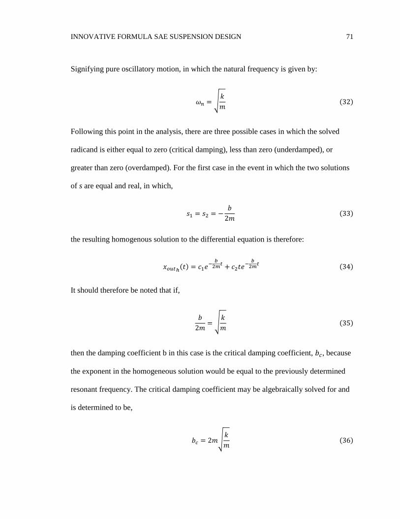
INNOVATIVE FORMULA SAE SUSPENSION DESIGN 71
Signifying pure oscillatory motion, in which the natural frequency is given by:
𝜔𝑛 = √𝑘
𝑚 (32)
Following this point in the analysis, there are three possible cases in which the solved
radicand is either equal to zero (critical damping), less than zero (underdamped), or
greater than zero (overdamped). For the first case in the event in which the two solutions
of s are equal and real, in which,
𝑠1 = 𝑠2 = −𝑏
2𝑚 (33)
the resulting homogenous solution to the differential equation is therefore:
𝑥𝑜𝑢𝑡ℎ(𝑡) = 𝑐1𝑒
−𝑏
2𝑚𝑡 + 𝑐2𝑡𝑒
−𝑏
2𝑚𝑡 (34)
It should therefore be noted that if,
𝑏
2𝑚= √
𝑘
𝑚 (35)
then the damping coefficient b in this case is the critical damping coefficient, 𝑏𝑐, because
the exponent in the homogeneous solution would be equal to the previously determined
resonant frequency. The critical damping coefficient may be algebraically solved for and
is determined to be,
𝑏𝑐 = 2𝑚√𝑘
𝑚 (36)

INNOVATIVE FORMULA SAE SUSPENSION DESIGN 72
Now a new term zeta may be introduced to simplify the relationship, being equal to the
ratio of the damping coefficient to the critical damping coefficient.
𝜁 =𝑏
𝑏𝑐=
𝑏
2𝑚𝜔𝑛 (37)
Now equation 4 may be re-written with the zeta variable as follows:
𝑠1,2 = 𝜁𝜔𝑛 ± 𝜔𝑛√𝜁2 − 1 (38)
The second case of the solution is one in which the radicand is less than zero, and there
exist two complex distinct roots as the solution to the above solution in equation 12,
given by
𝑠1,2 = −𝜁𝜔𝑛 ± 𝜔𝑛𝑗√1 − 𝜁2 (39)
This way the homogenous solution is given by:
𝑥𝑜𝑢𝑡ℎ(𝑡) = 𝑒−𝜁𝜔𝑛𝑡 {𝑐1 cos [(𝜔𝑛√1 − 𝜁2) 𝑡] + 𝑐2 sin [(𝜔𝑛√1 − 𝜁2) 𝑡]} (40)
And the final possibility is where the radicand is greater than zero, such that there exist 2
distinct real roots to the equation, given by
𝑠1,2 = −𝜁𝜔𝑛 ± 𝜔𝑛√𝜁2 − 1 (41)
In which the resulting homogenous solution is written simply as
𝑥𝑜𝑢𝑡ℎ(𝑡) = 𝑐1𝑒
(−𝜁𝜔𝑛+𝜔𝑛√𝜁2−1)𝑡+ 𝑐2𝑒
(−𝜁𝜔𝑛+𝜔𝑛√𝜁2−1)𝑡 (42)
The total solution then is to plot together the applicable case of the homogenous solution
with the particular solution, in which the particular solution is given as follows:
INNOVATIVE FORMULA SAE SUSPENSION DESIGN 73
𝑥𝑜𝑢𝑡𝑝=
𝐹𝑖𝑛
𝑘 (43)
𝑥𝑜𝑢𝑡𝑇𝑜𝑡𝑎𝑙= 𝑥𝑜𝑢𝑡ℎ
+ 𝑥𝑜𝑢𝑡𝑝 (44)

INNOVATIVE FORMULA SAE SUSPENSION DESIGN 74
Appendix B
MATLAB Code Generated for Four-Bar Linkage Analysis
% Suspension Geometry 4-bar Linkage Analysis
clear vars
%Required Characteristics for FSAE Design:
% Minimum wheel travel = 2.00 inches
% Minimum Jounce = 1.00 inch
% Minimum Rebound = 1.00 inch
%Set lengths of suspension members [all dimensions in inches] for 25% RC/CG height:
a = 13.71; % a = upper wishbone length
b = 8.08; % b = upright connection distance of wishbones
c = 14.84; % c = lower wishbone length
d = 6.0; % d = fixed distance between frame members mounting points
e = 0; % e = horiztonal displacement between top and bottom frame members
%f = 300/25.4; %total vertical height from absolute bottom frame member to top mounting
frame member
if c+b <= c+a
disp('Grashof Law Verified')
else
disp('Grashof Law Violated')
end
%Calculation of Position for the System:
theta_1 = 0; %by the way the diagram is drawn:
whl_trvl = 2.25;
% x = [0 e e+a*cosd(theta_4-theta_7-theta_2) c*cosd(theta_7) 0];
% y = [0 d*cosd(theta_5) d*cosd(theta_5)-a*sind(theta_4-theta_7-theta_2) c*sind(theta_7)
0];
% labels = {'Bottom Frame','Top Frame','Top of Upright','Bottom of Upright','Bottom
Frame'};
theta_2 = (80:105);
for theta_2 = (90:100)
K1 = d/a;
K2 = d/c;
K3 = (a^2 -b^2 +c^2 + d^2)/(2*a*c);
K4 = d/b;
K5 = (c^2-d^2-a^2-b^2)/(2*a*b);
A = cosd(theta_2)-K1-K2*cosd(theta_2)+K3;
B = -2*sind(theta_2);
C = K1-(K2+1)*cosd(theta_2) + K3;
D = cosd(theta_2)-K1 + K4*cosd(theta_2) +K5;
E = -2*sind(theta_2);
F = K1+(K4-1)*cosd(theta_2)+K5;
theta_3 = 2*atand((-E-(E^2-4*D*F)^0.5)/(2*D));
w = [0 a*sind(90-theta_2) a*sind(90-theta_2)+b*cosd(theta_3) d 0];
z = [0 a*cosd(90-theta_2) a*cosd(90-theta_2)+b*sind(theta_3) 0 0];
pause(0.02);
hold on
%Plot of all 4 links of suspension geometry through wheel travel
% subplot(2,2,1);
figure(1)
plot(w,z,'.-');
title('Suspension Geometry: Modeled as 4-bar Linkage');
xlabel('Vertical Distance [inches]');
ylabel('Horizontal Distance [inches]');
% text(x,y,labels,'VerticalAlignment','bottom','HorizontalAlignment','left');
axis([-10 18 -10 18]);
hold on

INNOVATIVE FORMULA SAE SUSPENSION DESIGN 75
%Plotting the axis of equilibrium ride height for desired ground clearance
grnd_clrnce = 1.5; %distance from ground surface to center of lowest frame member.
%desired actual ground clearance is 1.0 inches, to permit wheel travel of
%1in and retain clearance without vehicle contact to ground.
%Front Suspension Geometry
F_upper = 11.13; %height in inches from ground
F_lower = 4.63; %height in inches from ground
%Rear Suspension Geometry
R_upper = 10.74; %height in inches from ground
R_lower = 4.74; %height in inches from gound
d_tire = 16;
r_tire = d_tire/2;
h = r_tire - grnd_clrnce; %height of wheel center above bottom frame member
line([R_upper-r_tire,R_upper-r_tire], get(gca, 'ylim'));
text(R_upper-r_tire,-2,'\leftarrow Axis of Equilibrium Ride Height','FontSize',8);
%Plot of only Upright through wheel travel
upright_w = [a*sind(90-theta_2) a*sind(90-theta_2)+b*cosd(theta_3)];
upright_z = [a*cosd(90-theta_2) a*cosd(90-theta_2)+b*sind(theta_3)];
% subplot(2,2,2);
figure(2)
plot(upright_w,upright_z,'.-');
title('Close-Up of Exaggerated Upright Camber Angle Variation Throughout Wheel Travel')
xlabel('Vertical Distance [inches]');
ylabel('Horizontal Distance [inches]');
axis([-3 10 13 15.5]);
hold on
%Plotting the axis of equilibrium ride height for desired ground clearance
line([R_upper-r_tire,R_upper-r_tire], get(gca, 'ylim'));
text(R_upper-r_tire,5,'\leftarrow Axis of Equilibrium Ride Height','FontSize',8);
line([R_upper-r_tire+whl_trvl/2,R_upper-r_tire+whl_trvl/2], get(gca, 'ylim'));
text(R_upper-r_tire+whl_trvl/2,6,'\leftarrow Maximum Rebound Distance','FontSize',8);
line([R_upper-r_tire-whl_trvl/2,R_upper-r_tire-whl_trvl/2], get(gca, 'ylim'));
text(R_upper-r_tire-whl_trvl/2,4,'\leftarrow Maximum Jounce Distance','FontSize',8);
wheel_center = [(a*sind(90-theta_2)+a*sind(90-theta_2)+b*cosd(theta_3))/2 (a*cosd(90-
theta_2)+a*cosd(90-theta_2)+b*sind(theta_3))/2];
disp('wheel center coordinates:');
disp(wheel_center)
wheel_center_h = (a*sind(90-theta_2)+a*sind(90-theta_2)+b*cosd(theta_3))/2;
wheel_center_v = (a*cosd(90-theta_2)+a*cosd(90-theta_2)+b*sind(theta_3))/2;
% subplot(2,2,3);
figure(3)
plot(wheel_center_h,wheel_center_v,'.-');
title('Wheel Center Point through Wheel Travel');
xlabel('Vertical Position');
ylabel('Horizontal Position');
hold on
line([R_upper-r_tire,R_upper-r_tire], get(gca, 'ylim'));
line([R_upper-r_tire+whl_trvl/2,R_upper-r_tire+whl_trvl/2], get(gca, 'ylim'));
text(R_upper-r_tire+whl_trvl/2,10,'\leftarrow Maximum Rebound Distance','FontSize',8);
line([R_upper-r_tire-whl_trvl/2,R_upper-r_tire-whl_trvl/2], get(gca, 'ylim'));
text(R_upper-r_tire-whl_trvl/2,10.5,'\leftarrow Maximum Jounce Distance','FontSize',8);
axis([1 4.5 13.5 15]);
Initial_slope = 0;
%A plot of camber angle versus input theta_2
y2 = a*cosd(90-theta_2)+b*sind(theta_3);
y1 = a*cosd(90-theta_2);
x2 = a*sind(90-theta_2)+b*cosd(theta_3);
x1 = a*sind(90-theta_2);
hold on

INNOVATIVE FORMULA SAE SUSPENSION DESIGN 76
slope = (y2-y1)/(x2-x1)+Initial_slope;
camber = atand(slope)-8.3;
% subplot(2,2,4);
figure(4)
plot(theta_2, camber,'.-');
hold on
title('Camber Angle versus Theta 2');
xlabel('Theta 2 (degrees)');
ylabel('Camber Angle (degrees)');
%axis([70 95 2 8]);
end
%Putting labels on the final points to give reference to the plots
% subplot(2,2,1);
labels1 = {'Top Frame','Top of Upright','Bottom of Upright','Bottom Wishbone Mount','Top
Frame'};
text(w,z,labels1,'VerticalAlignment','bottom','HorizontalAlignment','left');
%subplot(2,2,2);
labels2 = {'Top of Upright','Bottom of Upright'};
text(upright_w,upright_z,labels2,'VerticalAlignment','bottom','HorizontalAlignment','left
');
%Listing output variables
theta_4 = 2*atand((-B-(B^2-4*A*C)^0.5)/(2*A));
%(These angles are for the proper orientation x-y attempt...)
% theta_5 = asind(e/a);
% theta_6 = theta_4-theta_2;
% theta_7 = 180-theta_4;
Angular_Position_Variables = {'theta_1'; 'theta_2'; 'theta_3'; 'theta_4'};
angles = [theta_1; theta_2; theta_3; theta_4];% theta_5; theta_6; theta_7];
T = table(Angular_Position_Variables, angles);
%calculating range of theta_2 that yields desired total wheel travel:
%calculate wheel center distance between first theta 2 input and last theta
%2 input
%Camber off-set to consider from inclination angle = 8.3 degrees

INNOVATIVE FORMULA SAE SUSPENSION DESIGN 77
Appendix C
MATLAB Code Generated for Dynamic Systems Vehicle Response Analysis
%Honors Petition Analysis
%Quarter Car Model:
syms S m_us m_s k b k_t omega
A_1 = [0 0 -1/m_us 0; 0 0 1/m_us -1/m_s; k_t -k -b/m_us b/m_s; 0 k b/m_us -b/m_s];
B_1 = [1 0 0 0];
sIA = S*eye(4)-A_1;
Num_1 = [sIA(:,1:3) B_1(:,1)];
%Transfer Function Vm/Vin
Vm_Vin = 1/m_s*det(Num_1)/det(sIA);
collect(Vm_Vin);
%Replace S with j*omega for harmonic input
TF1 = subs(Vm_Vin, S, omega*1i);
%Setting Values
m_us = 8; %kg
k = 4000; %N/m - this is the lowest available spring rate from KAZ tech, equivalent to
175lbf/in
k_t = 123464; %N/m
m_s = 182/4; %kg - for an estimated 400lb vehicle
b = 0.6*2*m_s*sqrt(k/m_s); %For damping ratio = 0.6
assume(omega, 'real');
TF1_num = -(k_t*(k + b*omega*1i));
TF1_denom = (k*m_s*omega^2 - k*k_t + k*m_us*omega^2 + k_t*m_s*omega^2 - m_s*m_us*omega^4
- b*k_t*omega*1i + b*m_s*omega^3*1i + b*m_us*omega^3*1i);
TF1_actual = TF1_num/TF1_denom;
%Amplitude Ratio and Phase Angle Calculations
amp_ratio_TF1 =
sqrt(real(TF1_num)^2+imag(TF1_num)^2)/sqrt(real(TF1_denom)^2+imag(TF1_denom)^2);
phi_1 = atan2d((imag(TF1_num)),real(TF1_num))-atan2d(imag(TF1_denom),real(TF1_denom));
phi_1 =subs(phi_1,omega,[0:1000]);
phi_1 = double(phi_1);
phi_1 = phi_1.* (phi_1 >= 0) + (phi_1 + 360) .* (phi_1 < 0);
figure(1);
subplot(2,1,1)
fplot(amp_ratio_TF1, [0 1000]);
title('Quarter Car Model Amplitude Ratio vs Frequency');
xlabel('Frequency [Hz]');
ylabel('Amplitude RatioTf V_m_s / V_i_n');
ylim([-.1 2.0]);
subplot(2,1,2);
plot(0:1000,phi_1);
title('Quarter Car Model Phase Angle Frequency Response');
xlabel('Frequency [Hz]');
ylabel('Phase Angle [deg]');
%%
%Conventional Transverse Half Car Model
syms S m_us1 m_us2 m_s b b_1 b_2 k k_1 k_2 k_t1 k_t2 V_in g omega
A_2 = [0 0 0 0 0 -1/m_us1 0 0; 0 0 0 0 0 1/m_us1 -1/m_s -1/m_s;
0 0 0 0 0 0 -1/m_s 1/m_us2; 0 0 0 0 0 0 0 1/m_us2;
0 0 0 0 0 1/m_us1 0 -1/m_us2; k_t1 -k_1 0 0 -k -b_1/m_us1 b_1/m_s 0;
0 k_1 k_2 0 0 b_1/m_us1 -(b_1-b_2)/m_s b_2/m_us2; 0 0 -k_2 -k_t2 k 0 b_2/m_s -
b_2/m_us2];
B_3 = [1 0 0 0; 0 0 0 0; 0 0 0 0; 0 0 0 0; 0 0 0 0; 0 1 0 0; 0 0 0 -1; 0 0 1 0];

INNOVATIVE FORMULA SAE SUSPENSION DESIGN 78
sIA = S*eye(8)-A_2;
%Transfer Function of Vmus1/Vin
Num_2 = [sIA(:,1:5),B_3(:,1),sIA(:,7:8)]; %Cramer's Rule: replacing the p_4 column with
V_in
TF2 = 1/m_us1*det(Num_2)/det(sIA);
collect(TF2);
%Transfer Function of Vmus2/Vin
Num_3 = [sIA(:,1:7),B_3(:,1)];
TF3 = 1/m_us2*det(Num_3)/det(sIA);
%Transfer Function of Vms/Vin
Num_4 = [sIA(:,1:6),B_3(:,1),sIA(:,8)];
TF4 = 1/m_s*det(Num_4)/det(sIA);
collect(TF4);
%Determining the Amplitude Ratio and Phase Angle Frequency Response of the
%Conventional Half Car Model Transfer Functions:
TF2 = subs(TF2, S, omega*1i);
TF3 = subs(TF3, S, omega*1i);
TF4 = subs(TF4, S, omega*1i);
%Assign values to symbolic parameters to give a plot for comparison:
%These values are made considering a typical FSAE racecar
m_s = 200; %kg
m_us1 = 8; %kg
m_us2 = m_us1; %kg
k_1 = 4000; %N/m
k_2 = k_1; %N/m
k_t1 = 123464; %N/m
k_t2 = k_t1; %N/m
k = 50000;
b_1 = 0.6*2*m_s/4*sqrt(k_1/(m_s/4)); %Should be between 0.5 and 0.7 damping ratio.
b_2 = b_1;
%Plotting Transfer Function 2, left unsprung mass velocity to V_in
TF2_num = -(k_t1*(2*b_2^2*m_s*omega^4 - b_2*m_s^2*omega^5*1i - k*m_s^2*omega^4 -
k_2*m_s^2*omega^4 - k_t2*m_s^2*omega^4 + m_s^2*m_us2*omega^6 - b_1*b_2*m_s*omega^4 +
b_1*k*m_s*omega^3*1i - b_2*k*m_s*omega^3*1i + b_1*k_2*m_s*omega^3*1i +
b_2*k_1*m_s*omega^3*1i - b_2*k_2*m_s*omega^3*2i + b_2*k_1*m_us2*omega^3*1i +
b_1*k_t2*m_s*omega^3*1i - b_2*k_t2*m_s*omega^3*1i - b_1*m_s*m_us2*omega^5*1i +
b_2*m_s*m_us2*omega^5*1i + k*k_1*m_s*omega^2 + k*k_2*m_s*omega^2 + k_1*k_2*m_s*omega^2 +
k_1*k_2*m_us2*omega^2 + k_1*k_t2*m_s*omega^2 + k_2*k_t2*m_s*omega^2 -
k_1*m_s*m_us2*omega^4 - k_2*m_s*m_us2*omega^4));
TF2_denom = (2*b_2^2*m_s*m_us1*omega^6 - b_1*b_2*m_s^2*omega^6 + b_1*k*m_s^2*omega^5*1i -
2*b_2^2*k*m_s*omega^4 + b_2*k*m_s^2*omega^5*1i - 2*b_2^2*k_1*m_s*omega^4 +
b_1*k_2*m_s^2*omega^5*1i + b_2*k_1*m_s^2*omega^5*1i - 2*b_2^2*k_t1*m_s*omega^4 +
b_1*k_t2*m_s^2*omega^5*1i + b_2*k_t1*m_s^2*omega^5*1i - b_1*b_2^2*m_s*omega^5*2i -
b_1*m_s^2*m_us2*omega^7*1i - b_2*m_s^2*m_us1*omega^7*1i + k*k_1*m_s^2*omega^4 +
k*k_2*m_s^2*omega^4 + k*k_t1*m_s^2*omega^4 + k*k_t2*m_s^2*omega^4 + k_1*k_2*m_s^2*omega^4
+ k_1*k_t2*m_s^2*omega^4 + k_2*k_t1*m_s^2*omega^4 + k_t1*k_t2*m_s^2*omega^4 -
k*m_s^2*m_us1*omega^6 - k*m_s^2*m_us2*omega^6 - k_1*m_s^2*m_us2*omega^6 -
k_2*m_s^2*m_us1*omega^6 - k_t1*m_s^2*m_us2*omega^6 - k_t2*m_s^2*m_us1*omega^6 +
m_s^2*m_us1*m_us2*omega^8 - 2*b_1*b_2*k*m_s*omega^4 - 2*b_1*b_2*k_2*m_s*omega^4 +
b_1*b_2*k_t1*m_s*omega^4 - b_1*b_2*k_t2*m_s*omega^4 - b_1*b_2*m_s*m_us1*omega^6 +
b_1*b_2*m_s*m_us2*omega^6 + b_2*k*k_1*m_s*omega^3*2i + b_2*k*k_2*m_s*omega^3*2i -
b_2*k*k_1*m_us2*omega^3*2i - b_1*k*k_t1*m_s*omega^3*1i - b_1*k*k_t2*m_s*omega^3*1i +
b_2*k*k_t1*m_s*omega^3*1i + b_2*k*k_t2*m_s*omega^3*1i + b_2*k_1*k_2*m_s*omega^3*2i -
b_1*k_2*k_t1*m_s*omega^3*1i - b_2*k_1*k_t1*m_s*omega^3*1i - b_1*k_2*k_t2*m_s*omega^3*1i +
b_2*k_1*k_t2*m_s*omega^3*1i + b_2*k_2*k_t1*m_s*omega^3*2i - b_2*k_1*k_t1*m_us2*omega^3*1i
- b_1*k_t1*k_t2*m_s*omega^3*1i + b_2*k_t1*k_t2*m_s*omega^3*1i +
b_1*k*m_s*m_us1*omega^5*1i + b_1*k*m_s*m_us2*omega^5*1i - b_2*k*m_s*m_us1*omega^5*1i -
b_2*k*m_s*m_us2*omega^5*1i + b_1*k_2*m_s*m_us1*omega^5*1i + b_2*k_1*m_s*m_us1*omega^5*1i
+ b_1*k_2*m_s*m_us2*omega^5*1i - b_2*k_1*m_s*m_us2*omega^5*1i -
b_2*k_2*m_s*m_us1*omega^5*2i + b_2*k_1*m_us1*m_us2*omega^5*1i +
b_1*k_t1*m_s*m_us2*omega^5*1i + b_1*k_t2*m_s*m_us1*omega^5*1i -
b_2*k_t1*m_s*m_us2*omega^5*1i - b_2*k_t2*m_s*m_us1*omega^5*1i -

INNOVATIVE FORMULA SAE SUSPENSION DESIGN 79
b_1*m_s*m_us1*m_us2*omega^7*1i + b_2*m_s*m_us1*m_us2*omega^7*1i - k*k_1*k_t1*m_s*omega^2
- k*k_1*k_t2*m_s*omega^2 - k*k_2*k_t1*m_s*omega^2 - k*k_2*k_t2*m_s*omega^2 -
k_1*k_2*k_t1*m_s*omega^2 - k_1*k_2*k_t2*m_s*omega^2 - k_1*k_2*k_t1*m_us2*omega^2 -
k_1*k_t1*k_t2*m_s*omega^2 - k_2*k_t1*k_t2*m_s*omega^2 + k*k_1*m_s*m_us1*omega^4 +
k*k_2*m_s*m_us1*omega^4 + k*k_2*m_s*m_us2*omega^4 + k_1*k_2*m_s*m_us1*omega^4 +
k_1*k_2*m_s*m_us2*omega^4 + k_1*k_2*m_us1*m_us2*omega^4 + k_1*k_t1*m_s*m_us2*omega^4 +
k_1*k_t2*m_s*m_us1*omega^4 + k_2*k_t1*m_s*m_us2*omega^4 + k_2*k_t2*m_s*m_us1*omega^4 -
k_1*m_s*m_us1*m_us2*omega^6 - k_2*m_s*m_us1*m_us2*omega^6);
TF2_actual = TF2_num/TF2_denom;
% H2 = tf([-56937720257911902017945600000000 -3819498389416736554363503247360000i
3506737252964536091714189532186536543 151045883307874263858068069490434806976i -
74997029763368346898221501022877676397339 -2012966146597960745377582809939607156765866i
561096677042127519547757619417240724567297966
37209735545605006698306619193361073923567616i -
44238226098683991777087695400023451811545964544
1722010398720942306000393237584310330982400000i
877489276075031452779253757246774968320000000000],[3689348814741910323200000000 0 -
291797976455567166397935396635342 0 9050216191234562096011300626214101788 0 -
127139589893816555139911723637762535244094 0
735097324995800450811324296348669012956987392 0 -
57550527568803929465446408905987755443662880768 0
1137420930565652810071563351290617528320000000000]);
% figure(3);
% bode(H2);
% title('Conventional Half Car Model Bode Diagram of V_m_u_s_1/V_i_n');
amp_ratio_TF2 =
sqrt((real(TF2_num))^2+(imag(TF2_num))^2)/sqrt((real(TF2_denom))^2+(imag(TF2_denom))^2);
figure(4);
subplot(2,1,1);
fplot(amp_ratio_TF2,[0,1000]);
title('Conventional Half Car Model Amplitude Ratio of V_m_u_s_1 / V_i_n');
xlabel('Frequency [Hz]');
ylabel('Amplitude Ratio of V_m_u_s_1 / V_i_n');
ylim([0 1.75]);
phi_2 = atan2d((imag(TF2_num)),real(TF2_num))-atan2d(imag(TF2_denom),real(TF2_denom));
phi_2 =subs(phi_2,omega,[0:1000]);
phi_2 = double(phi_2);
phi_2 = phi_2.* (phi_2 >= 0) + (phi_2 + 360) .* (phi_2 < 0);
subplot(2,1,2);
plot(0:1000,phi_2);
title('Conventional Half Car Model Phase Angle of V_m_u_s_1 / V_i_n');
xlabel('Frequency [Hz]');
ylabel('Phase Angle [deg]');
%Plotting Transfer Function 3, right unsprung mass Velocity to V_in
TF3_num = -(k_t1*m_s*omega*(k*m_s*omega^3*1i - k*k_1*omega*1i - k*k_2*omega*1i -
k_1*k_2*omega*1i + b_1*b_2*omega^3*1i + b_1*k*omega^2 - b_2*k*omega^2 + b_1*k_2*omega^2 +
b_2*k_1*omega^2)*1i);
TF3_denom = (2*b_2^2*m_s*m_us1*omega^6 - b_1*b_2*m_s^2*omega^6 + b_1*k*m_s^2*omega^5*1i -
2*b_2^2*k*m_s*omega^4 + b_2*k*m_s^2*omega^5*1i - 2*b_2^2*k_1*m_s*omega^4 +
b_1*k_2*m_s^2*omega^5*1i + b_2*k_1*m_s^2*omega^5*1i - 2*b_2^2*k_t1*m_s*omega^4 +
b_1*k_t2*m_s^2*omega^5*1i + b_2*k_t1*m_s^2*omega^5*1i - b_1*b_2^2*m_s*omega^5*2i -
b_1*m_s^2*m_us2*omega^7*1i - b_2*m_s^2*m_us1*omega^7*1i + k*k_1*m_s^2*omega^4 +
k*k_2*m_s^2*omega^4 + k*k_t1*m_s^2*omega^4 + k*k_t2*m_s^2*omega^4 + k_1*k_2*m_s^2*omega^4
+ k_1*k_t2*m_s^2*omega^4 + k_2*k_t1*m_s^2*omega^4 + k_t1*k_t2*m_s^2*omega^4 -
k*m_s^2*m_us1*omega^6 - k*m_s^2*m_us2*omega^6 - k_1*m_s^2*m_us2*omega^6 -
k_2*m_s^2*m_us1*omega^6 - k_t1*m_s^2*m_us2*omega^6 - k_t2*m_s^2*m_us1*omega^6 +
m_s^2*m_us1*m_us2*omega^8 - 2*b_1*b_2*k*m_s*omega^4 - 2*b_1*b_2*k_2*m_s*omega^4 +
b_1*b_2*k_t1*m_s*omega^4 - b_1*b_2*k_t2*m_s*omega^4 - b_1*b_2*m_s*m_us1*omega^6 +
b_1*b_2*m_s*m_us2*omega^6 + b_2*k*k_1*m_s*omega^3*2i + b_2*k*k_2*m_s*omega^3*2i -
b_2*k*k_1*m_us2*omega^3*2i - b_1*k*k_t1*m_s*omega^3*1i - b_1*k*k_t2*m_s*omega^3*1i +
b_2*k*k_t1*m_s*omega^3*1i + b_2*k*k_t2*m_s*omega^3*1i + b_2*k_1*k_2*m_s*omega^3*2i -
b_1*k_2*k_t1*m_s*omega^3*1i - b_2*k_1*k_t1*m_s*omega^3*1i - b_1*k_2*k_t2*m_s*omega^3*1i +
b_2*k_1*k_t2*m_s*omega^3*1i + b_2*k_2*k_t1*m_s*omega^3*2i - b_2*k_1*k_t1*m_us2*omega^3*1i
- b_1*k_t1*k_t2*m_s*omega^3*1i + b_2*k_t1*k_t2*m_s*omega^3*1i +
b_1*k*m_s*m_us1*omega^5*1i + b_1*k*m_s*m_us2*omega^5*1i - b_2*k*m_s*m_us1*omega^5*1i -
b_2*k*m_s*m_us2*omega^5*1i + b_1*k_2*m_s*m_us1*omega^5*1i + b_2*k_1*m_s*m_us1*omega^5*1i

INNOVATIVE FORMULA SAE SUSPENSION DESIGN 80
+ b_1*k_2*m_s*m_us2*omega^5*1i - b_2*k_1*m_s*m_us2*omega^5*1i -
b_2*k_2*m_s*m_us1*omega^5*2i + b_2*k_1*m_us1*m_us2*omega^5*1i +
b_1*k_t1*m_s*m_us2*omega^5*1i + b_1*k_t2*m_s*m_us1*omega^5*1i -
b_2*k_t1*m_s*m_us2*omega^5*1i - b_2*k_t2*m_s*m_us1*omega^5*1i -
b_1*m_s*m_us1*m_us2*omega^7*1i + b_2*m_s*m_us1*m_us2*omega^7*1i - k*k_1*k_t1*m_s*omega^2
- k*k_1*k_t2*m_s*omega^2 - k*k_2*k_t1*m_s*omega^2 - k*k_2*k_t2*m_s*omega^2 -
k_1*k_2*k_t1*m_s*omega^2 - k_1*k_2*k_t2*m_s*omega^2 - k_1*k_2*k_t1*m_us2*omega^2 -
k_1*k_t1*k_t2*m_s*omega^2 - k_2*k_t1*k_t2*m_s*omega^2 + k*k_1*m_s*m_us1*omega^4 +
k*k_2*m_s*m_us1*omega^4 + k*k_2*m_s*m_us2*omega^4 + k_1*k_2*m_s*m_us1*omega^4 +
k_1*k_2*m_s*m_us2*omega^4 + k_1*k_2*m_us1*m_us2*omega^4 + k_1*k_t1*m_s*m_us2*omega^4 +
k_1*k_t2*m_s*m_us1*omega^4 + k_2*k_t1*m_s*m_us2*omega^4 + k_2*k_t2*m_s*m_us1*omega^4 -
k_1*m_s*m_us1*m_us2*omega^6 - k_2*m_s*m_us1*m_us2*omega^6);
TF3_actual = TF3_num/TF3_denom;
amp_ratio_TF3 =
sqrt((real(TF3_num))^2+(imag(TF3_num))^2)/sqrt((real(TF3_denom))^2+(imag(TF3_denom))^2);
% figure(5);
% H3 = tf([1464438165033494136472618401792000000,
195863877409290252677973733408329303525*1i, -71069840071612843540548377317557308533450, -
4301395089965414876537350139078609409597775*1i,
651628432086768101407606450390502562224777200, -
145563079048854427592038881035805667652096000*1i, -
52039244978822833689677944100460585884232908800,
12707123512235269799761546958005306654720000000*1i +
1039726617962485429169238376175370240000000000000],[14757395258967641292800000000, 0, -
1167191905822268665591741586541368, 0, 36200864764938248384045202504856407152, 0, -
508558359575266220559646894551050140976376, 0,
2940389299983201803245297185394676051827949568, 0, -
230202110275215717861785635623951021774651523072, 0,
4549683722262611240286253405162470113280000000000]);
% bode(H3);
% title('Conventional Half Car Model Bode Diagram V_m_u_s_2/V_i_n')
% figure(6);
% bode(H2);
% hold on
% bode(H3);
% p1=bode(H2);
% p2=bode(H3);
% title('Conventional Half Car Model Left and Right Wheel Frequency Response');
% legend([p1 p2],'V_m_u_s_1/V_i_n','V_m_u_s_2/V_i_n');
figure(7);
subplot(2,1,1);
fplot(amp_ratio_TF3,[0,1000]);
title('Conventional Half Car Model Amplitude Ratio of V_m_u_s_2 / V_i_n');
xlabel('Frequency [Hz]');
ylabel('Amplitude Ratio of V_m_u_s_2 / V_i_n');
ylim([0 1]);
phi_3 = atan2d((imag(TF3_num)),real(TF3_num))-atan2d(imag(TF3_denom),real(TF3_denom));
phi_3 =subs(phi_3,omega,[0:1000]);
phi_3 = double(phi_3);
phi_3 = phi_3.* (phi_3 >= 0) + (phi_3 + 360) .* (phi_3 < 0);
subplot(2,1,2);
plot(0:1000,phi_3);
title('Conventional Half Car Model Phase Angle of V_m_u_s_2 / V_i_n');
xlabel('Frequency [Hz]');
ylabel('Phase Angle [deg]');
%Plotting Transfer Function 4, sprung mass velocity to V_in
TF4_num = -(k_t1*(k*k_1*m_s*omega^2 + b_1*k*m_s*omega^3*1i + b_2*k*m_s*omega^3*1i +
b_1*k_2*m_s*omega^3*1i + b_2*k_1*m_s*omega^3*1i + b_1*k_t2*m_s*omega^3*1i -
b_1*m_s*m_us2*omega^5*1i - b_1*b_2*m_s*omega^4 + k*k_2*m_s*omega^2 - k*k_1*m_us2*omega^2
+ k_1*k_2*m_s*omega^2 + k_1*k_t2*m_s*omega^2 - k_1*m_s*m_us2*omega^4));
TF4_denom = (2*b_2^2*m_s*m_us1*omega^6 - b_1*b_2*m_s^2*omega^6 + b_1*k*m_s^2*omega^5*1i -
2*b_2^2*k*m_s*omega^4 + b_2*k*m_s^2*omega^5*1i - 2*b_2^2*k_1*m_s*omega^4 +
b_1*k_2*m_s^2*omega^5*1i + b_2*k_1*m_s^2*omega^5*1i - 2*b_2^2*k_t1*m_s*omega^4 +
b_1*k_t2*m_s^2*omega^5*1i + b_2*k_t1*m_s^2*omega^5*1i - b_1*b_2^2*m_s*omega^5*2i -
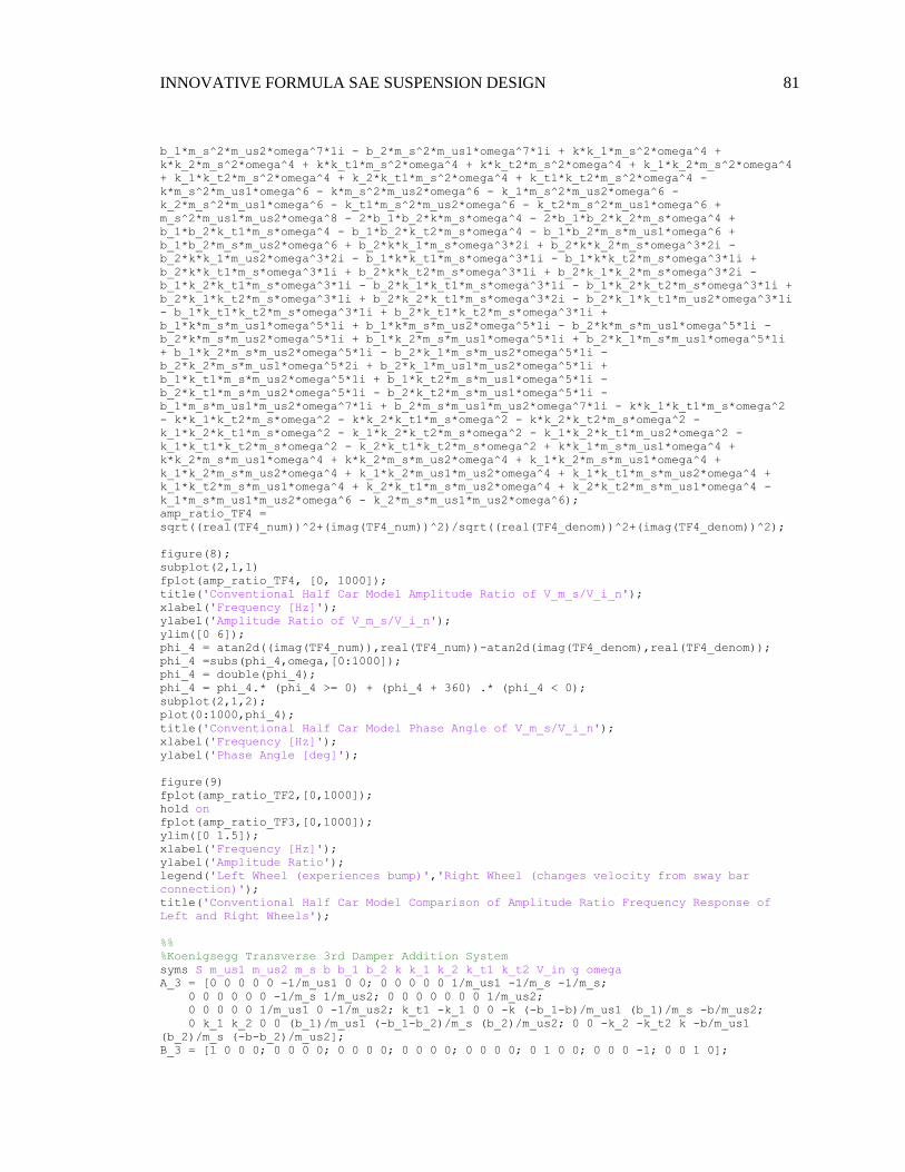
INNOVATIVE FORMULA SAE SUSPENSION DESIGN 81
b_1*m_s^2*m_us2*omega^7*1i - b_2*m_s^2*m_us1*omega^7*1i + k*k_1*m_s^2*omega^4 +
k*k_2*m_s^2*omega^4 + k*k_t1*m_s^2*omega^4 + k*k_t2*m_s^2*omega^4 + k_1*k_2*m_s^2*omega^4
+ k_1*k_t2*m_s^2*omega^4 + k_2*k_t1*m_s^2*omega^4 + k_t1*k_t2*m_s^2*omega^4 -
k*m_s^2*m_us1*omega^6 - k*m_s^2*m_us2*omega^6 - k_1*m_s^2*m_us2*omega^6 -
k_2*m_s^2*m_us1*omega^6 - k_t1*m_s^2*m_us2*omega^6 - k_t2*m_s^2*m_us1*omega^6 +
m_s^2*m_us1*m_us2*omega^8 - 2*b_1*b_2*k*m_s*omega^4 - 2*b_1*b_2*k_2*m_s*omega^4 +
b_1*b_2*k_t1*m_s*omega^4 - b_1*b_2*k_t2*m_s*omega^4 - b_1*b_2*m_s*m_us1*omega^6 +
b_1*b_2*m_s*m_us2*omega^6 + b_2*k*k_1*m_s*omega^3*2i + b_2*k*k_2*m_s*omega^3*2i -
b_2*k*k_1*m_us2*omega^3*2i - b_1*k*k_t1*m_s*omega^3*1i - b_1*k*k_t2*m_s*omega^3*1i +
b_2*k*k_t1*m_s*omega^3*1i + b_2*k*k_t2*m_s*omega^3*1i + b_2*k_1*k_2*m_s*omega^3*2i -
b_1*k_2*k_t1*m_s*omega^3*1i - b_2*k_1*k_t1*m_s*omega^3*1i - b_1*k_2*k_t2*m_s*omega^3*1i +
b_2*k_1*k_t2*m_s*omega^3*1i + b_2*k_2*k_t1*m_s*omega^3*2i - b_2*k_1*k_t1*m_us2*omega^3*1i
- b_1*k_t1*k_t2*m_s*omega^3*1i + b_2*k_t1*k_t2*m_s*omega^3*1i +
b_1*k*m_s*m_us1*omega^5*1i + b_1*k*m_s*m_us2*omega^5*1i - b_2*k*m_s*m_us1*omega^5*1i -
b_2*k*m_s*m_us2*omega^5*1i + b_1*k_2*m_s*m_us1*omega^5*1i + b_2*k_1*m_s*m_us1*omega^5*1i
+ b_1*k_2*m_s*m_us2*omega^5*1i - b_2*k_1*m_s*m_us2*omega^5*1i -
b_2*k_2*m_s*m_us1*omega^5*2i + b_2*k_1*m_us1*m_us2*omega^5*1i +
b_1*k_t1*m_s*m_us2*omega^5*1i + b_1*k_t2*m_s*m_us1*omega^5*1i -
b_2*k_t1*m_s*m_us2*omega^5*1i - b_2*k_t2*m_s*m_us1*omega^5*1i -
b_1*m_s*m_us1*m_us2*omega^7*1i + b_2*m_s*m_us1*m_us2*omega^7*1i - k*k_1*k_t1*m_s*omega^2
- k*k_1*k_t2*m_s*omega^2 - k*k_2*k_t1*m_s*omega^2 - k*k_2*k_t2*m_s*omega^2 -
k_1*k_2*k_t1*m_s*omega^2 - k_1*k_2*k_t2*m_s*omega^2 - k_1*k_2*k_t1*m_us2*omega^2 -
k_1*k_t1*k_t2*m_s*omega^2 - k_2*k_t1*k_t2*m_s*omega^2 + k*k_1*m_s*m_us1*omega^4 +
k*k_2*m_s*m_us1*omega^4 + k*k_2*m_s*m_us2*omega^4 + k_1*k_2*m_s*m_us1*omega^4 +
k_1*k_2*m_s*m_us2*omega^4 + k_1*k_2*m_us1*m_us2*omega^4 + k_1*k_t1*m_s*m_us2*omega^4 +
k_1*k_t2*m_s*m_us1*omega^4 + k_2*k_t1*m_s*m_us2*omega^4 + k_2*k_t2*m_s*m_us1*omega^4 -
k_1*m_s*m_us1*m_us2*omega^6 - k_2*m_s*m_us1*m_us2*omega^6);
amp_ratio_TF4 =
sqrt((real(TF4_num))^2+(imag(TF4_num))^2)/sqrt((real(TF4_denom))^2+(imag(TF4_denom))^2);
figure(8);
subplot(2,1,1)
fplot(amp_ratio_TF4, [0, 1000]);
title('Conventional Half Car Model Amplitude Ratio of V_m_s/V_i_n');
xlabel('Frequency [Hz]');
ylabel('Amplitude Ratio of V_m_s/V_i_n');
ylim([0 6]);
phi_4 = atan2d((imag(TF4_num)),real(TF4_num))-atan2d(imag(TF4_denom),real(TF4_denom));
phi_4 =subs(phi_4,omega,[0:1000]);
phi_4 = double(phi_4);
phi_4 = phi_4.* (phi_4 >= 0) + (phi_4 + 360) .* (phi_4 < 0);
subplot(2,1,2);
plot(0:1000,phi_4);
title('Conventional Half Car Model Phase Angle of V_m_s/V_i_n');
xlabel('Frequency [Hz]');
ylabel('Phase Angle [deg]');
figure(9)
fplot(amp_ratio_TF2,[0,1000]);
hold on
fplot(amp_ratio_TF3,[0,1000]);
ylim([0 1.5]);
xlabel('Frequency [Hz]');
ylabel('Amplitude Ratio');
legend('Left Wheel (experiences bump)','Right Wheel (changes velocity from sway bar
connection)');
title('Conventional Half Car Model Comparison of Amplitude Ratio Frequency Response of
Left and Right Wheels');
%%
%Koenigsegg Transverse 3rd Damper Addition System
syms S m_us1 m_us2 m_s b b_1 b_2 k k_1 k_2 k_t1 k_t2 V_in g omega
A_3 = [0 0 0 0 0 -1/m_us1 0 0; 0 0 0 0 0 1/m_us1 -1/m_s -1/m_s;
0 0 0 0 0 0 -1/m_s 1/m_us2; 0 0 0 0 0 0 0 1/m_us2;
0 0 0 0 0 1/m_us1 0 -1/m_us2; k_t1 -k_1 0 0 -k (-b_1-b)/m_us1 (b_1)/m_s -b/m_us2;
0 k_1 k_2 0 0 (b_1)/m_us1 (-b_1-b_2)/m_s (b_2)/m_us2; 0 0 -k_2 -k_t2 k -b/m_us1
(b_2)/m_s (-b-b_2)/m_us2];
B_3 = [1 0 0 0; 0 0 0 0; 0 0 0 0; 0 0 0 0; 0 0 0 0; 0 1 0 0; 0 0 0 -1; 0 0 1 0];
INNOVATIVE FORMULA SAE SUSPENSION DESIGN 82
sIA = S*eye(8)-A_3;
det(sIA);
%Transfer Function of Vmus1/Vin
Num_5 = [sIA(:,1:5),B_3(:,1),sIA(:,7:8)]; %Cramer's Rule: replacing the p_4 column with
V_in
TF5 = 1/m_us1*det(Num_5)/det(sIA);
collect(TF5);
%Transfer Function of Vmus2/Vin
Num_6 = [sIA(:,1:7),B_3(:,1)];
TF6 = 1/m_us2*det(Num_6)/det(sIA);
%Transfer Function of Vms/Vin
Num_7 = [sIA(:,1:6),B_3(:,1),sIA(:,8)];
TF7 = 1/m_s*det(Num_7)/det(sIA);
collect(TF4);
%Determining the Amplitude Ratio and Phase Angle Frequency Response of the
%Conventional Half Car Model Transfer Functions:
TF5 = subs(TF5, S, omega*1i);
TF6 = subs(TF6, S, omega*1i);
TF7 = subs(TF7, S, omega*1i);
%Assign values to symbolic parameters to give a plot for comparison:
%These values are made considering a typical FSAE racecar
m_s = 200; %kg
m_us1 = 8; %kg
m_us2 = m_us1; %kg
k_1 = 4000; %N/m
k_2 = k_1; %N/m
k_t1 = 123464; %N/m
k_t2 = k_t1; %N/m
k = 50000;
b_1 = 0.707*2*m_s/4*sqrt(k_1/(m_s/4)); %Damping ratio should be between 0.5 and 0.7
b_2 = b_1;
b = 1*b_1;
%Plotting Transfer Function 5, left unsprung mass velocity to V_in
TF5_num = (k_t1*(m_s^2*m_us2*omega^6 - b_2*m_s^2*omega^5*1i - k*m_s^2*omega^4 -
k_2*m_s^2*omega^4 - k_t2*m_s^2*omega^4 - b*m_s^2*omega^5*1i + b*k*m_s*omega^3*1i +
b*k_1*m_s*omega^3*1i + b_2*k*m_s*omega^3*1i + b*k_1*m_us2*omega^3*1i +
b*k_t2*m_s*omega^3*1i + b_2*k_1*m_s*omega^3*1i + b_2*k_1*m_us2*omega^3*1i +
b_2*k_t2*m_s*omega^3*1i - b*m_s*m_us2*omega^5*1i - b_2*m_s*m_us2*omega^5*1i +
k*k_1*m_s*omega^2 + k*k_2*m_s*omega^2 + k_1*k_2*m_s*omega^2 + k_1*k_2*m_us2*omega^2 +
k_1*k_t2*m_s*omega^2 + k_2*k_t2*m_s*omega^2 - k_1*m_s*m_us2*omega^4 -
k_2*m_s*m_us2*omega^4));
TF5_denom = (b*b_1^2*m_s*omega^5*1i + b*b_1*m_s^2*omega^6 + b*b_2*m_s^2*omega^6 +
b_1^2*b_2*m_s*omega^5*1i + b_1*b_2*m_s^2*omega^6 - b*k*m_s^2*omega^5*4i +
b_1^2*k*m_s*omega^4 - b*k_1*m_s^2*omega^5*1i - b_1*k*m_s^2*omega^5*1i -
b*k_2*m_s^2*omega^5*1i - b_2*k*m_s^2*omega^5*1i - b*k_t1*m_s^2*omega^5*1i -
b*k_t2*m_s^2*omega^5*1i + b_1^2*k_2*m_s*omega^4 - b_1*k_2*m_s^2*omega^5*1i -
b_2*k_1*m_s^2*omega^5*1i + b_1^2*k_t2*m_s*omega^4 - b_1*k_t2*m_s^2*omega^5*1i -
b_2*k_t1*m_s^2*omega^5*1i + b*m_s^2*m_us1*omega^7*1i + b*m_s^2*m_us2*omega^7*1i -
b_1^2*m_s*m_us2*omega^6 + b_1*m_s^2*m_us2*omega^7*1i + b_2*m_s^2*m_us1*omega^7*1i -
k*k_1*m_s^2*omega^4 - k*k_2*m_s^2*omega^4 - k*k_t1*m_s^2*omega^4 - k*k_t2*m_s^2*omega^4 -
k_1*k_2*m_s^2*omega^4 - k_1*k_t2*m_s^2*omega^4 - k_2*k_t1*m_s^2*omega^4 -
k_t1*k_t2*m_s^2*omega^4 + k*m_s^2*m_us1*omega^6 + k*m_s^2*m_us2*omega^6 +
k_1*m_s^2*m_us2*omega^6 + k_2*m_s^2*m_us1*omega^6 + k_t1*m_s^2*m_us2*omega^6 +
k_t2*m_s^2*m_us1*omega^6 - m_s^2*m_us1*m_us2*omega^8 + 3*b*b_1*k*m_s*omega^4 -
b*b_2*k*m_s*omega^4 + b*b_1*k_1*m_s*omega^4 - b*b_2*k_1*m_s*omega^4 +
b_1*b_2*k*m_s*omega^4 + b*b_1*k_1*m_us2*omega^4 - b*b_2*k_1*m_us2*omega^4 +
b*b_1*k_t2*m_s*omega^4 - b*b_2*k_t2*m_s*omega^4 + b_1*b_2*k_1*m_s*omega^4 -
b_1*b_2*k_t2*m_s*omega^4 - b*b_1*m_s*m_us2*omega^6 + b*b_2*m_s*m_us2*omega^6 +
b_1*b_2*m_s*m_us2*omega^6 + b*k*k_1*m_s*omega^3*1i + b*k*k_2*m_s*omega^3*1i +
b*k*k_1*m_us2*omega^3*1i + b*k*k_t1*m_s*omega^3*1i + b*k*k_t2*m_s*omega^3*1i -
b_1*k*k_1*m_s*omega^3*1i + b*k_1*k_2*m_s*omega^3*1i - b_1*k*k_2*m_s*omega^3*1i +
b_1*k*k_1*m_us2*omega^3*1i + b*k_1*k_2*m_us2*omega^3*1i + b*k_1*k_t1*m_s*omega^3*1i +

INNOVATIVE FORMULA SAE SUSPENSION DESIGN 83
b_2*k*k_t1*m_s*omega^3*1i + b*k_2*k_t2*m_s*omega^3*1i + b_2*k*k_t2*m_s*omega^3*1i +
b*k_1*k_t1*m_us2*omega^3*1i + b*k_t1*k_t2*m_s*omega^3*1i - b_1*k_1*k_2*m_s*omega^3*1i -
b_1*k_1*k_t2*m_s*omega^3*1i + b_2*k_1*k_t1*m_s*omega^3*1i + b_1*k_2*k_t2*m_s*omega^3*1i +
b_2*k_1*k_t2*m_s*omega^3*1i + b_2*k_1*k_t1*m_us2*omega^3*1i +
b_2*k_t1*k_t2*m_s*omega^3*1i - b*k*m_s*m_us1*omega^5*1i - b*k*m_s*m_us2*omega^5*1i -
b*k_1*m_s*m_us1*omega^5*1i - b*k_1*m_s*m_us2*omega^5*1i - b_2*k*m_s*m_us1*omega^5*1i -
b*k_2*m_s*m_us2*omega^5*1i - b_2*k*m_s*m_us2*omega^5*1i - b*k_1*m_us1*m_us2*omega^5*1i -
b*k_t1*m_s*m_us2*omega^5*1i - b*k_t2*m_s*m_us1*omega^5*1i + b_1*k_1*m_s*m_us2*omega^5*1i
- b_2*k_1*m_s*m_us1*omega^5*1i - b_1*k_2*m_s*m_us2*omega^5*1i -
b_2*k_1*m_s*m_us2*omega^5*1i - b_2*k_1*m_us1*m_us2*omega^5*1i -
b_2*k_t1*m_s*m_us2*omega^5*1i - b_2*k_t2*m_s*m_us1*omega^5*1i +
b*m_s*m_us1*m_us2*omega^7*1i + b_2*m_s*m_us1*m_us2*omega^7*1i + k*k_1*k_t1*m_s*omega^2 +
k*k_1*k_t2*m_s*omega^2 + k*k_2*k_t1*m_s*omega^2 + k*k_2*k_t2*m_s*omega^2 +
k_1*k_2*k_t1*m_s*omega^2 + k_1*k_2*k_t2*m_s*omega^2 + k_1*k_2*k_t1*m_us2*omega^2 +
k_1*k_t1*k_t2*m_s*omega^2 + k_2*k_t1*k_t2*m_s*omega^2 - k*k_1*m_s*m_us1*omega^4 -
k*k_2*m_s*m_us1*omega^4 - k*k_2*m_s*m_us2*omega^4 - k_1*k_2*m_s*m_us1*omega^4 -
k_1*k_2*m_s*m_us2*omega^4 - k_1*k_2*m_us1*m_us2*omega^4 - k_1*k_t1*m_s*m_us2*omega^4 -
k_1*k_t2*m_s*m_us1*omega^4 - k_2*k_t1*m_s*m_us2*omega^4 - k_2*k_t2*m_s*m_us1*omega^4 +
k_1*m_s*m_us1*m_us2*omega^6 + k_2*m_s*m_us1*m_us2*omega^6);
amp_ratio_TF5 =
sqrt((real(TF5_num))^2+(imag(TF5_num))^2)/sqrt((real(TF5_denom))^2+(imag(TF5_denom))^2);
figure(10);
subplot(2,1,1);
fplot(amp_ratio_TF5,[0,1000]);
title('Transverse Damper Half Car Model Amplitude Ratio of V_m_u_s_1 / V_i_n');
xlabel('Frequency [Hz]');
ylabel('Amplitude Ratio of V_m_u_s_1 / V_i_n');
ylim([0 1.75]);
phi_5 = atan2d((imag(TF5_num)),real(TF5_num))-atan2d(imag(TF5_denom),real(TF5_denom));
phi_5 =subs(phi_5,omega,[0:1000]);
phi_5 = double(phi_5);
phi_5 = phi_5.* (phi_5 >= 0) + (phi_5 + 360) .* (phi_5 < 0);
subplot(2,1,2);
plot(0:1000,phi_5);
title('Transferse Damper Half Car Model Phase Angle of V_m_u_s_1 / V_i_n');
xlabel('Frequency [Hz]');
ylabel('Phase Angle [deg]');
%Plotting Transfer Function 7, right unsprung mass Velocity to V_in
TF6_num = (k_t1*m_s*omega*(k*m_s*omega^3*1i - k*k_1*omega*1i - k*k_2*omega*1i -
k_1*k_2*omega*1i + b*b_1*omega^3*1i + b_1*b_2*omega^3*1i + b*k*omega^2 + b_2*k*omega^2 +
b_1*k_2*omega^2 + b_2*k_1*omega^2 + b*m_s*omega^4)*1i);
TF6_denom = (b*b_1^2*m_s*omega^5*1i + b*b_1*m_s^2*omega^6 + b*b_2*m_s^2*omega^6 +
b_1^2*b_2*m_s*omega^5*1i + b_1*b_2*m_s^2*omega^6 - b*k*m_s^2*omega^5*4i +
b_1^2*k*m_s*omega^4 - b*k_1*m_s^2*omega^5*1i - b_1*k*m_s^2*omega^5*1i -
b*k_2*m_s^2*omega^5*1i - b_2*k*m_s^2*omega^5*1i - b*k_t1*m_s^2*omega^5*1i -
b*k_t2*m_s^2*omega^5*1i + b_1^2*k_2*m_s*omega^4 - b_1*k_2*m_s^2*omega^5*1i -
b_2*k_1*m_s^2*omega^5*1i + b_1^2*k_t2*m_s*omega^4 - b_1*k_t2*m_s^2*omega^5*1i -
b_2*k_t1*m_s^2*omega^5*1i + b*m_s^2*m_us1*omega^7*1i + b*m_s^2*m_us2*omega^7*1i -
b_1^2*m_s*m_us2*omega^6 + b_1*m_s^2*m_us2*omega^7*1i + b_2*m_s^2*m_us1*omega^7*1i -
k*k_1*m_s^2*omega^4 - k*k_2*m_s^2*omega^4 - k*k_t1*m_s^2*omega^4 - k*k_t2*m_s^2*omega^4 -
k_1*k_2*m_s^2*omega^4 - k_1*k_t2*m_s^2*omega^4 - k_2*k_t1*m_s^2*omega^4 -
k_t1*k_t2*m_s^2*omega^4 + k*m_s^2*m_us1*omega^6 + k*m_s^2*m_us2*omega^6 +
k_1*m_s^2*m_us2*omega^6 + k_2*m_s^2*m_us1*omega^6 + k_t1*m_s^2*m_us2*omega^6 +
k_t2*m_s^2*m_us1*omega^6 - m_s^2*m_us1*m_us2*omega^8 + 3*b*b_1*k*m_s*omega^4 -
b*b_2*k*m_s*omega^4 + b*b_1*k_1*m_s*omega^4 - b*b_2*k_1*m_s*omega^4 +
b_1*b_2*k*m_s*omega^4 + b*b_1*k_1*m_us2*omega^4 - b*b_2*k_1*m_us2*omega^4 +
b*b_1*k_t2*m_s*omega^4 - b*b_2*k_t2*m_s*omega^4 + b_1*b_2*k_1*m_s*omega^4 -
b_1*b_2*k_t2*m_s*omega^4 - b*b_1*m_s*m_us2*omega^6 + b*b_2*m_s*m_us2*omega^6 +
b_1*b_2*m_s*m_us2*omega^6 + b*k*k_1*m_s*omega^3*1i + b*k*k_2*m_s*omega^3*1i +
b*k*k_1*m_us2*omega^3*1i + b*k*k_t1*m_s*omega^3*1i + b*k*k_t2*m_s*omega^3*1i -
b_1*k*k_1*m_s*omega^3*1i + b*k_1*k_2*m_s*omega^3*1i - b_1*k*k_2*m_s*omega^3*1i +
b_1*k*k_1*m_us2*omega^3*1i + b*k_1*k_2*m_us2*omega^3*1i + b*k_1*k_t1*m_s*omega^3*1i +
b_2*k*k_t1*m_s*omega^3*1i + b*k_2*k_t2*m_s*omega^3*1i + b_2*k*k_t2*m_s*omega^3*1i +
b*k_1*k_t1*m_us2*omega^3*1i + b*k_t1*k_t2*m_s*omega^3*1i - b_1*k_1*k_2*m_s*omega^3*1i -
b_1*k_1*k_t2*m_s*omega^3*1i + b_2*k_1*k_t1*m_s*omega^3*1i + b_1*k_2*k_t2*m_s*omega^3*1i +
b_2*k_1*k_t2*m_s*omega^3*1i + b_2*k_1*k_t1*m_us2*omega^3*1i +

INNOVATIVE FORMULA SAE SUSPENSION DESIGN 84
b_2*k_t1*k_t2*m_s*omega^3*1i - b*k*m_s*m_us1*omega^5*1i - b*k*m_s*m_us2*omega^5*1i -
b*k_1*m_s*m_us1*omega^5*1i - b*k_1*m_s*m_us2*omega^5*1i - b_2*k*m_s*m_us1*omega^5*1i -
b*k_2*m_s*m_us2*omega^5*1i - b_2*k*m_s*m_us2*omega^5*1i - b*k_1*m_us1*m_us2*omega^5*1i -
b*k_t1*m_s*m_us2*omega^5*1i - b*k_t2*m_s*m_us1*omega^5*1i + b_1*k_1*m_s*m_us2*omega^5*1i
- b_2*k_1*m_s*m_us1*omega^5*1i - b_1*k_2*m_s*m_us2*omega^5*1i -
b_2*k_1*m_s*m_us2*omega^5*1i - b_2*k_1*m_us1*m_us2*omega^5*1i -
b_2*k_t1*m_s*m_us2*omega^5*1i - b_2*k_t2*m_s*m_us1*omega^5*1i +
b*m_s*m_us1*m_us2*omega^7*1i + b_2*m_s*m_us1*m_us2*omega^7*1i + k*k_1*k_t1*m_s*omega^2 +
k*k_1*k_t2*m_s*omega^2 + k*k_2*k_t1*m_s*omega^2 + k*k_2*k_t2*m_s*omega^2 +
k_1*k_2*k_t1*m_s*omega^2 + k_1*k_2*k_t2*m_s*omega^2 + k_1*k_2*k_t1*m_us2*omega^2 +
k_1*k_t1*k_t2*m_s*omega^2 + k_2*k_t1*k_t2*m_s*omega^2 - k*k_1*m_s*m_us1*omega^4 -
k*k_2*m_s*m_us1*omega^4 - k*k_2*m_s*m_us2*omega^4 - k_1*k_2*m_s*m_us1*omega^4 -
k_1*k_2*m_s*m_us2*omega^4 - k_1*k_2*m_us1*m_us2*omega^4 - k_1*k_t1*m_s*m_us2*omega^4 -
k_1*k_t2*m_s*m_us1*omega^4 - k_2*k_t1*m_s*m_us2*omega^4 - k_2*k_t2*m_s*m_us1*omega^4 +
k_1*m_s*m_us1*m_us2*omega^6 + k_2*m_s*m_us1*m_us2*omega^6);
amp_ratio_TF6 =
sqrt((real(TF6_num))^2+(imag(TF6_num))^2)/sqrt((real(TF6_denom))^2+(imag(TF6_denom))^2);
figure(11);
subplot(2,1,1);
fplot(amp_ratio_TF6,[0,1000]);
title('Transverse Damper Half Car Model Amplitude Ratio of V_m_u_s_2 / V_i_n');
xlabel('Frequency [Hz]');
ylabel('Amplitude Ratio of V_m_u_s_2 / V_i_n');
ylim([0 1]);
phi_6 = atan2d((imag(TF6_num)),real(TF6_num))-atan2d(imag(TF6_denom),real(TF6_denom));
phi_6 =subs(phi_6,omega,[0:1000]);
phi_6 = double(phi_6);
phi_6 = phi_6.* (phi_6 >= 0) + (phi_6 + 360) .* (phi_6 < 0);
subplot(2,1,2);
plot(0:1000,phi_6);
title('Transverse Damper Half Car Model Phase Angle of V_m_u_s_2 / V_i_n');
xlabel('Frequency [Hz]');
ylabel('Phase Angle [deg]');
%Plotting Transfer Function 8, sprung mass velocity to V_in
TF7_num = (k_t1*(k*k_1*m_s*omega^2 - b_1*b_2*m_s*omega^4 + b*k*m_s*omega^3*2i +
b*k_1*m_s*omega^3*1i + b_1*k*m_s*omega^3*1i + b_2*k*m_s*omega^3*1i +
b*k_1*m_us2*omega^3*1i + b*k_t2*m_s*omega^3*1i + b_1*k_2*m_s*omega^3*1i +
b_2*k_1*m_s*omega^3*1i + b_1*k_t2*m_s*omega^3*1i - b*m_s*m_us2*omega^5*1i -
b_1*m_s*m_us2*omega^5*1i - b*b_1*m_s*omega^4 + k*k_2*m_s*omega^2 - k*k_1*m_us2*omega^2 +
k_1*k_2*m_s*omega^2 + k_1*k_t2*m_s*omega^2 - k_1*m_s*m_us2*omega^4));
TF7_denom = (b*b_1^2*m_s*omega^5*1i + b*b_1*m_s^2*omega^6 + b*b_2*m_s^2*omega^6 +
b_1^2*b_2*m_s*omega^5*1i + b_1*b_2*m_s^2*omega^6 - b*k*m_s^2*omega^5*4i +
b_1^2*k*m_s*omega^4 - b*k_1*m_s^2*omega^5*1i - b_1*k*m_s^2*omega^5*1i -
b*k_2*m_s^2*omega^5*1i - b_2*k*m_s^2*omega^5*1i - b*k_t1*m_s^2*omega^5*1i -
b*k_t2*m_s^2*omega^5*1i + b_1^2*k_2*m_s*omega^4 - b_1*k_2*m_s^2*omega^5*1i -
b_2*k_1*m_s^2*omega^5*1i + b_1^2*k_t2*m_s*omega^4 - b_1*k_t2*m_s^2*omega^5*1i -
b_2*k_t1*m_s^2*omega^5*1i + b*m_s^2*m_us1*omega^7*1i + b*m_s^2*m_us2*omega^7*1i -
b_1^2*m_s*m_us2*omega^6 + b_1*m_s^2*m_us2*omega^7*1i + b_2*m_s^2*m_us1*omega^7*1i -
k*k_1*m_s^2*omega^4 - k*k_2*m_s^2*omega^4 - k*k_t1*m_s^2*omega^4 - k*k_t2*m_s^2*omega^4 -
k_1*k_2*m_s^2*omega^4 - k_1*k_t2*m_s^2*omega^4 - k_2*k_t1*m_s^2*omega^4 -
k_t1*k_t2*m_s^2*omega^4 + k*m_s^2*m_us1*omega^6 + k*m_s^2*m_us2*omega^6 +
k_1*m_s^2*m_us2*omega^6 + k_2*m_s^2*m_us1*omega^6 + k_t1*m_s^2*m_us2*omega^6 +
k_t2*m_s^2*m_us1*omega^6 - m_s^2*m_us1*m_us2*omega^8 + 3*b*b_1*k*m_s*omega^4 -
b*b_2*k*m_s*omega^4 + b*b_1*k_1*m_s*omega^4 - b*b_2*k_1*m_s*omega^4 +
b_1*b_2*k*m_s*omega^4 + b*b_1*k_1*m_us2*omega^4 - b*b_2*k_1*m_us2*omega^4 +
b*b_1*k_t2*m_s*omega^4 - b*b_2*k_t2*m_s*omega^4 + b_1*b_2*k_1*m_s*omega^4 -
b_1*b_2*k_t2*m_s*omega^4 - b*b_1*m_s*m_us2*omega^6 + b*b_2*m_s*m_us2*omega^6 +
b_1*b_2*m_s*m_us2*omega^6 + b*k*k_1*m_s*omega^3*1i + b*k*k_2*m_s*omega^3*1i +
b*k*k_1*m_us2*omega^3*1i + b*k*k_t1*m_s*omega^3*1i + b*k*k_t2*m_s*omega^3*1i -
b_1*k*k_1*m_s*omega^3*1i + b*k_1*k_2*m_s*omega^3*1i - b_1*k*k_2*m_s*omega^3*1i +
b_1*k*k_1*m_us2*omega^3*1i + b*k_1*k_2*m_us2*omega^3*1i + b*k_1*k_t1*m_s*omega^3*1i +
b_2*k*k_t1*m_s*omega^3*1i + b*k_2*k_t2*m_s*omega^3*1i + b_2*k*k_t2*m_s*omega^3*1i +
b*k_1*k_t1*m_us2*omega^3*1i + b*k_t1*k_t2*m_s*omega^3*1i - b_1*k_1*k_2*m_s*omega^3*1i -
b_1*k_1*k_t2*m_s*omega^3*1i + b_2*k_1*k_t1*m_s*omega^3*1i + b_1*k_2*k_t2*m_s*omega^3*1i +
b_2*k_1*k_t2*m_s*omega^3*1i + b_2*k_1*k_t1*m_us2*omega^3*1i +
b_2*k_t1*k_t2*m_s*omega^3*1i - b*k*m_s*m_us1*omega^5*1i - b*k*m_s*m_us2*omega^5*1i -

INNOVATIVE FORMULA SAE SUSPENSION DESIGN 85
b*k_1*m_s*m_us1*omega^5*1i - b*k_1*m_s*m_us2*omega^5*1i - b_2*k*m_s*m_us1*omega^5*1i -
b*k_2*m_s*m_us2*omega^5*1i - b_2*k*m_s*m_us2*omega^5*1i - b*k_1*m_us1*m_us2*omega^5*1i -
b*k_t1*m_s*m_us2*omega^5*1i - b*k_t2*m_s*m_us1*omega^5*1i + b_1*k_1*m_s*m_us2*omega^5*1i
- b_2*k_1*m_s*m_us1*omega^5*1i - b_1*k_2*m_s*m_us2*omega^5*1i -
b_2*k_1*m_s*m_us2*omega^5*1i - b_2*k_1*m_us1*m_us2*omega^5*1i -
b_2*k_t1*m_s*m_us2*omega^5*1i - b_2*k_t2*m_s*m_us1*omega^5*1i +
b*m_s*m_us1*m_us2*omega^7*1i + b_2*m_s*m_us1*m_us2*omega^7*1i + k*k_1*k_t1*m_s*omega^2 +
k*k_1*k_t2*m_s*omega^2 + k*k_2*k_t1*m_s*omega^2 + k*k_2*k_t2*m_s*omega^2 +
k_1*k_2*k_t1*m_s*omega^2 + k_1*k_2*k_t2*m_s*omega^2 + k_1*k_2*k_t1*m_us2*omega^2 +
k_1*k_t1*k_t2*m_s*omega^2 + k_2*k_t1*k_t2*m_s*omega^2 - k*k_1*m_s*m_us1*omega^4 -
k*k_2*m_s*m_us1*omega^4 - k*k_2*m_s*m_us2*omega^4 - k_1*k_2*m_s*m_us1*omega^4 -
k_1*k_2*m_s*m_us2*omega^4 - k_1*k_2*m_us1*m_us2*omega^4 - k_1*k_t1*m_s*m_us2*omega^4 -
k_1*k_t2*m_s*m_us1*omega^4 - k_2*k_t1*m_s*m_us2*omega^4 - k_2*k_t2*m_s*m_us1*omega^4 +
k_1*m_s*m_us1*m_us2*omega^6 + k_2*m_s*m_us1*m_us2*omega^6);
amp_ratio_TF7 =
sqrt((real(TF7_num))^2+(imag(TF7_num))^2)/sqrt((real(TF7_denom))^2+(imag(TF7_denom))^2);
figure(12);
subplot(2,1,1)
fplot(amp_ratio_TF7,[0 1000]);
title('Transverse Damper Half Car Model Amplitude Ratio of V_m_s / V_i_n');
xlabel('Frequency [Hz]');
ylabel('Amplitude Ratio of V_m_s / V_i_n');
ylim([0 2]);
phi_7 = atan2d((imag(TF7_num)),real(TF7_num))-atan2d(imag(TF7_denom),real(TF7_denom));
phi_7 =subs(phi_7,omega,[0:1000]);
phi_7 = double(phi_7);
phi_7 = phi_7.* (phi_7 >= 0) + (phi_7 + 360) .* (phi_7 < 0);
subplot(2,1,2);
plot(0:1000,phi_7);
title('Transverse Damper Half Car Model Phase Angle of V_m_s / V_i_n');
xlabel('Frequency [Hz]');
ylabel('Phase Angle [deg]');
figure(13)
fplot(amp_ratio_TF5,[0,1000]);
hold on
fplot(amp_ratio_TF6,[0,1000]);
ylim([0 1.5]);
xlabel('Frequency [Hz]');
ylabel('Amplitude Ratio');
legend('Left Wheel (experiences bump)','Right Wheel (changes velocity from sway bar
connection damped by transverse damper)');
title('Transverse Damper Half Car Model Comparison of Amplitude Ratio Frequency Response
of Left and Right Wheels');
figure (14)
fplot(amp_ratio_TF6,[0,1000]);
hold on
fplot(amp_ratio_TF3,[0,1000]);
xlabel('Frequency [Hz]');
ylabel('Amplitude Ratio');
legend('Right Wheel with Transverse Damper','Right Wheel Without Transverse Damper');
title('Comparison of Right Wheel Amplitude Ratio Frequency Response With and Without
Transverse Damper');
%Plotting Frequency Response of Transverse Damper System with Various
%Damping Coefficients
figure (15);
for b = 0*b_1:0.2*b_1:3*b_1
TF6_num = (k_t1*m_s*omega*(k*m_s*omega^3*1i - k*k_1*omega*1i - k*k_2*omega*1i -
k_1*k_2*omega*1i + b*b_1*omega^3*1i + b_1*b_2*omega^3*1i + b*k*omega^2 + b_2*k*omega^2 +
b_1*k_2*omega^2 + b_2*k_1*omega^2 + b*m_s*omega^4)*1i);
TF6_denom = (b*b_1^2*m_s*omega^5*1i + b*b_1*m_s^2*omega^6 + b*b_2*m_s^2*omega^6 +
b_1^2*b_2*m_s*omega^5*1i + b_1*b_2*m_s^2*omega^6 - b*k*m_s^2*omega^5*4i +
b_1^2*k*m_s*omega^4 - b*k_1*m_s^2*omega^5*1i - b_1*k*m_s^2*omega^5*1i -
b*k_2*m_s^2*omega^5*1i - b_2*k*m_s^2*omega^5*1i - b*k_t1*m_s^2*omega^5*1i -
b*k_t2*m_s^2*omega^5*1i + b_1^2*k_2*m_s*omega^4 - b_1*k_2*m_s^2*omega^5*1i -

INNOVATIVE FORMULA SAE SUSPENSION DESIGN 86
b_2*k_1*m_s^2*omega^5*1i + b_1^2*k_t2*m_s*omega^4 - b_1*k_t2*m_s^2*omega^5*1i -
b_2*k_t1*m_s^2*omega^5*1i + b*m_s^2*m_us1*omega^7*1i + b*m_s^2*m_us2*omega^7*1i -
b_1^2*m_s*m_us2*omega^6 + b_1*m_s^2*m_us2*omega^7*1i + b_2*m_s^2*m_us1*omega^7*1i -
k*k_1*m_s^2*omega^4 - k*k_2*m_s^2*omega^4 - k*k_t1*m_s^2*omega^4 - k*k_t2*m_s^2*omega^4 -
k_1*k_2*m_s^2*omega^4 - k_1*k_t2*m_s^2*omega^4 - k_2*k_t1*m_s^2*omega^4 -
k_t1*k_t2*m_s^2*omega^4 + k*m_s^2*m_us1*omega^6 + k*m_s^2*m_us2*omega^6 +
k_1*m_s^2*m_us2*omega^6 + k_2*m_s^2*m_us1*omega^6 + k_t1*m_s^2*m_us2*omega^6 +
k_t2*m_s^2*m_us1*omega^6 - m_s^2*m_us1*m_us2*omega^8 + 3*b*b_1*k*m_s*omega^4 -
b*b_2*k*m_s*omega^4 + b*b_1*k_1*m_s*omega^4 - b*b_2*k_1*m_s*omega^4 +
b_1*b_2*k*m_s*omega^4 + b*b_1*k_1*m_us2*omega^4 - b*b_2*k_1*m_us2*omega^4 +
b*b_1*k_t2*m_s*omega^4 - b*b_2*k_t2*m_s*omega^4 + b_1*b_2*k_1*m_s*omega^4 -
b_1*b_2*k_t2*m_s*omega^4 - b*b_1*m_s*m_us2*omega^6 + b*b_2*m_s*m_us2*omega^6 +
b_1*b_2*m_s*m_us2*omega^6 + b*k*k_1*m_s*omega^3*1i + b*k*k_2*m_s*omega^3*1i +
b*k*k_1*m_us2*omega^3*1i + b*k*k_t1*m_s*omega^3*1i + b*k*k_t2*m_s*omega^3*1i -
b_1*k*k_1*m_s*omega^3*1i + b*k_1*k_2*m_s*omega^3*1i - b_1*k*k_2*m_s*omega^3*1i +
b_1*k*k_1*m_us2*omega^3*1i + b*k_1*k_2*m_us2*omega^3*1i + b*k_1*k_t1*m_s*omega^3*1i +
b_2*k*k_t1*m_s*omega^3*1i + b*k_2*k_t2*m_s*omega^3*1i + b_2*k*k_t2*m_s*omega^3*1i +
b*k_1*k_t1*m_us2*omega^3*1i + b*k_t1*k_t2*m_s*omega^3*1i - b_1*k_1*k_2*m_s*omega^3*1i -
b_1*k_1*k_t2*m_s*omega^3*1i + b_2*k_1*k_t1*m_s*omega^3*1i + b_1*k_2*k_t2*m_s*omega^3*1i +
b_2*k_1*k_t2*m_s*omega^3*1i + b_2*k_1*k_t1*m_us2*omega^3*1i +
b_2*k_t1*k_t2*m_s*omega^3*1i - b*k*m_s*m_us1*omega^5*1i - b*k*m_s*m_us2*omega^5*1i -
b*k_1*m_s*m_us1*omega^5*1i - b*k_1*m_s*m_us2*omega^5*1i - b_2*k*m_s*m_us1*omega^5*1i -
b*k_2*m_s*m_us2*omega^5*1i - b_2*k*m_s*m_us2*omega^5*1i - b*k_1*m_us1*m_us2*omega^5*1i -
b*k_t1*m_s*m_us2*omega^5*1i - b*k_t2*m_s*m_us1*omega^5*1i + b_1*k_1*m_s*m_us2*omega^5*1i
- b_2*k_1*m_s*m_us1*omega^5*1i - b_1*k_2*m_s*m_us2*omega^5*1i -
b_2*k_1*m_s*m_us2*omega^5*1i - b_2*k_1*m_us1*m_us2*omega^5*1i -
b_2*k_t1*m_s*m_us2*omega^5*1i - b_2*k_t2*m_s*m_us1*omega^5*1i +
b*m_s*m_us1*m_us2*omega^7*1i + b_2*m_s*m_us1*m_us2*omega^7*1i + k*k_1*k_t1*m_s*omega^2 +
k*k_1*k_t2*m_s*omega^2 + k*k_2*k_t1*m_s*omega^2 + k*k_2*k_t2*m_s*omega^2 +
k_1*k_2*k_t1*m_s*omega^2 + k_1*k_2*k_t2*m_s*omega^2 + k_1*k_2*k_t1*m_us2*omega^2 +
k_1*k_t1*k_t2*m_s*omega^2 + k_2*k_t1*k_t2*m_s*omega^2 - k*k_1*m_s*m_us1*omega^4 -
k*k_2*m_s*m_us1*omega^4 - k*k_2*m_s*m_us2*omega^4 - k_1*k_2*m_s*m_us1*omega^4 -
k_1*k_2*m_s*m_us2*omega^4 - k_1*k_2*m_us1*m_us2*omega^4 - k_1*k_t1*m_s*m_us2*omega^4 -
k_1*k_t2*m_s*m_us1*omega^4 - k_2*k_t1*m_s*m_us2*omega^4 - k_2*k_t2*m_s*m_us1*omega^4 +
k_1*m_s*m_us1*m_us2*omega^6 + k_2*m_s*m_us1*m_us2*omega^6);
amp_ratio_TF6MR =
sqrt((real(TF6_num))^2+(imag(TF6_num))^2)/sqrt((real(TF6_denom))^2+(imag(TF6_denom))^2);
fplot(amp_ratio_TF6MR, [0 600]);
legend('Right Wheel with Transverse Damper')
hold on
end
Legend = cell(16,1);
Legend{1} = 'b = 0.0*b_1';
Legend{2} = 'b = 0.2*b_1';
Legend{3} = 'b = 0.4*b_1';
Legend{4} = 'b = 0.6*b_1';
Legend{5} = 'b = 0.8*b_1';
Legend{6} = 'b = 1.0*b_1';
Legend{7} = 'b = 1.2*b_1';
Legend{8} = 'b = 1.4*b_1';
Legend{9} = 'b = 1.6*b_1';
Legend{10} = 'b = 1.8*b_1';
Legend{11} = 'b = 2.0*b_1';
Legend{12} = 'b = 2.2*b_1';
Legend{13} = 'b = 2.4*b_1';
Legend{14} = 'b = 2.6*b_1';
Legend{15} = 'b = 2.8*b_1';
Legend{16} = 'b = 3.0*b_1';
legend(Legend);
title('Frequency Response of Right Wheel from Left Wheel Disturbance in 3rd Damper
System, Over Many Transverse Damping Coefficients');
xlabel('Freqency [Hz]');
ylabel('Amplitude Ratio');
INNOVATIVE FORMULA SAE SUSPENSION DESIGN 87
Appendix D
Hand Calculations and Derivations of Dynamic Systems Analysis