Japanese Monetary Policy during the Collapse of the Bubble ...

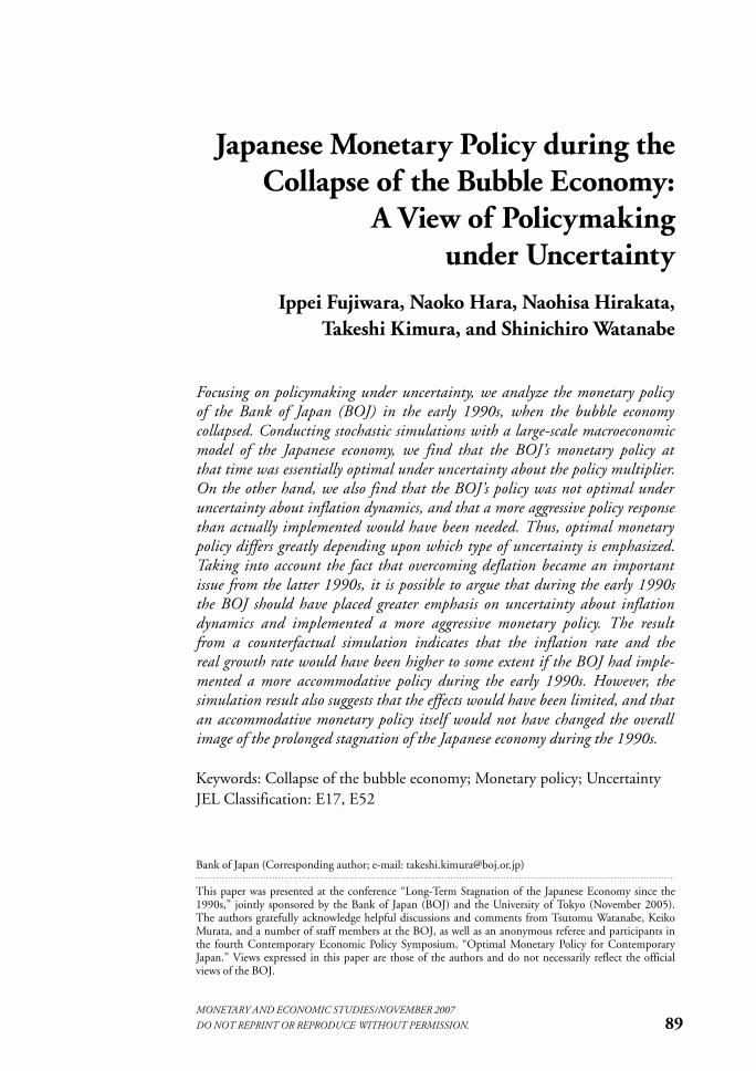
89

Japanese Monetary Policy during the

Collapse of the Bubble Economy:

A View of Policymaking

under Uncertainty

Ippei Fujiwara, Naoko Hara, Naohisa Hirakata,

Takeshi Kimura, and Shinichiro Watanabe

Focusing on policymaking under uncertainty, we analyze the monetary policy

of the Bank of Japan (BOJ) in the early 1990s, when the bubble economy

collapsed. Conducting stochastic simulations with a large-scale macroeconomic

model of the Japanese economy, we find that the BOJ’s monetary policy at

that time was essentially optimal under uncertainty about the policy multiplier.

On the other hand, we also find that the BOJ’s policy was not optimal under

uncertainty about inflation dynamics, and that a more aggressive policy response

than actually implemented would have been needed. Thus, optimal monetary

policy differs greatly depending upon which type of uncertainty is emphasized.

Taking into account the fact that overcoming deflation became an important

issue from the latter 1990s, it is possible to argue that during the early 1990s

the BOJ should have placed greater emphasis on uncertainty about inflation

dynamics and implemented a more aggressive monetary policy. The result

from a counterfactual simulation indicates that the inflation rate and the

real growth rate would have been higher to some extent if the BOJ had imple-

mented a more accommodative policy during the early 1990s. However, the

simulation result also suggests that the effects would have been limited, and that

an accommodative monetary policy itself would not have changed the overall

image of the prolonged stagnation of the Japanese economy during the 1990s.

Keywords: Collapse of the bubble economy; Monetary policy; Uncertainty

JEL Classification: E17, E52

MONETARY AND ECONOMIC STUDIES/NOVEMBER 2007

DO NOT REPRINT OR REPRODUCE WITHOUT PERMISSION.

Bank of Japan (Corresponding author; e-mail: [email protected])

This paper was presented at the conference “Long-Term Stagnation of the Japanese Economy since the1990s,” jointly sponsored by the Bank of Japan (BOJ) and the University of Tokyo (November 2005).The authors gratefully acknowledge helpful discussions and comments from Tsutomu Watanabe, KeikoMurata, and a number of staff members at the BOJ, as well as an anonymous referee and participants inthe fourth Contemporary Economic Policy Symposium, “Optimal Monetary Policy for ContemporaryJapan.” Views expressed in this paper are those of the authors and do not necessarily reflect the officialviews of the BOJ.

I. Introduction

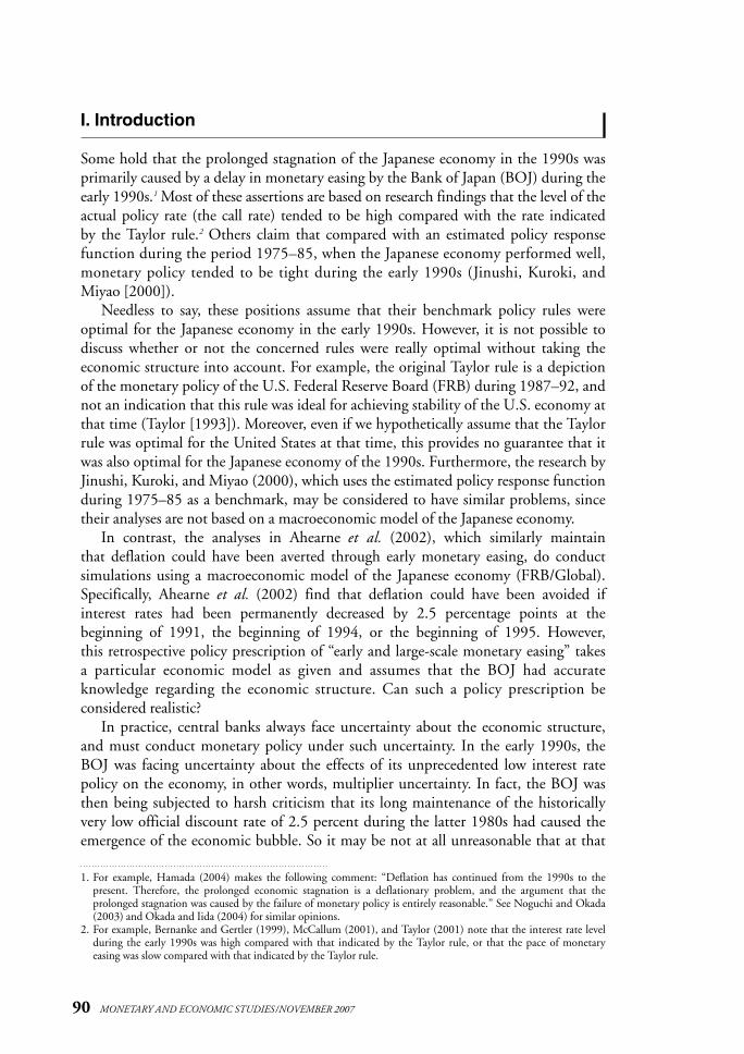
Some hold that the prolonged stagnation of the Japanese economy in the 1990s was

primarily caused by a delay in monetary easing by the Bank of Japan (BOJ) during the

early 1990s.1 Most of these assertions are based on research findings that the level of the

actual policy rate (the call rate) tended to be high compared with the rate indicated

by the Taylor rule.2 Others claim that compared with an estimated policy response

function during the period 1975–85, when the Japanese economy performed well,

monetary policy tended to be tight during the early 1990s (Jinushi, Kuroki, and

Miyao [2000]).

Needless to say, these positions assume that their benchmark policy rules were

optimal for the Japanese economy in the early 1990s. However, it is not possible to

discuss whether or not the concerned rules were really optimal without taking the

economic structure into account. For example, the original Taylor rule is a depiction

of the monetary policy of the U.S. Federal Reserve Board (FRB) during 1987–92, and

not an indication that this rule was ideal for achieving stability of the U.S. economy at

that time (Taylor [1993]). Moreover, even if we hypothetically assume that the Taylor

rule was optimal for the United States at that time, this provides no guarantee that it

was also optimal for the Japanese economy of the 1990s. Furthermore, the research by

Jinushi, Kuroki, and Miyao (2000), which uses the estimated policy response function

during 1975–85 as a benchmark, may be considered to have similar problems, since

their analyses are not based on a macroeconomic model of the Japanese economy.

In contrast, the analyses in Ahearne et al. (2002), which similarly maintain

that deflation could have been averted through early monetary easing, do conduct

simulations using a macroeconomic model of the Japanese economy (FRB/Global).

Specifically, Ahearne et al. (2002) find that deflation could have been avoided if

interest rates had been permanently decreased by 2.5 percentage points at the

beginning of 1991, the beginning of 1994, or the beginning of 1995. However,

this retrospective policy prescription of “early and large-scale monetary easing” takes

a particular economic model as given and assumes that the BOJ had accurate

knowledge regarding the economic structure. Can such a policy prescription be

considered realistic?

In practice, central banks always face uncertainty about the economic structure,

and must conduct monetary policy under such uncertainty. In the early 1990s, the

BOJ was facing uncertainty about the effects of its unprecedented low interest rate

policy on the economy, in other words, multiplier uncertainty. In fact, the BOJ was

then being subjected to harsh criticism that its long maintenance of the historically

very low official discount rate of 2.5 percent during the latter 1980s had caused the

emergence of the economic bubble. So it may be not at all unreasonable that at that

90 MONETARY AND ECONOMIC STUDIES/NOVEMBER 2007

1. For example, Hamada (2004) makes the following comment: “Deflation has continued from the 1990s to the present. Therefore, the prolonged economic stagnation is a deflationary problem, and the argument that the prolonged stagnation was caused by the failure of monetary policy is entirely reasonable.” See Noguchi and Okada(2003) and Okada and Iida (2004) for similar opinions.

2. For example, Bernanke and Gertler (1999), McCallum (2001), and Taylor (2001) note that the interest rate levelduring the early 1990s was high compared with that indicated by the Taylor rule, or that the pace of monetary easing was slow compared with that indicated by the Taylor rule.

time the BOJ was hesitant about dropping interest rates below 2.5 percent and par-

ticularly cautious regarding the risks of diverse side effects if low interest rates were

maintained for a long period of time. Some suggest that when faced with this sort of

multiplier uncertainty, it is desirable for the authorities to implement conservative

monetary policy (Brainard [1967]). Specifically, when “Brainard conservatism” is

considered, the BOJ’s decision to cautiously advance monetary easing in the early

1990s can be theoretically justified.

Based on all the above points, to evaluate the BOJ’s monetary policy during the

early 1990s it is necessary not only to use a macroeconomic model of the Japanese

economy, but also to implement analyses that consider the uncertainty confronting

the BOJ. There are various types of uncertainty aside from multiplier uncertainty,

such as uncertainty about the inflation process and about the persistence of demand

shocks. Hence we need to evaluate whether the BOJ, while considering such uncer-

tainty regarding the economic structure, could have or should have implemented

monetary easing earlier in terms of a real-time policy judgment.

Based on this awareness of the issues, we evaluate the BOJ’s monetary policy

during the early 1990s by introducing the uncertainty regarding the economic struc-

ture into the Japanese Economic Model (JEM), a quantitative macroeconomic model

developed by the BOJ’s Research and Statistics Department. In this paper, we employ

two approaches that the authorities can utilize for policy conduct, facing uncertainty

about the parameters of the economic structure. The first is to aim at minimizing the

expected loss, given a prior belief about the distribution of uncertain parameters.

Hereafter, for convenience this is referred to as the “Bayesian approach.” The second

approach is to adopt the best policy assuming the parameter values that cause the worst-

case scenario for the authorities within the some range of uncertain parameters. This

is referred to as the “minimax approach” (or the “robust approach”) in the sense that

it aims at minimizing the maximum loss. This paper evaluates the BOJ’s policy via

stochastic simulations based on these two approaches. The four main conclusions

reached are as follows

(1) The stochastic simulation using the JEM suggests that the BOJ’s monetary

policy during the early 1990s was essentially optimal under uncertainty about

the policy multiplier. This conclusion holds under both the Bayesian and the

minimax approaches.

(2) On the other hand, the BOJ’s policy at that time was not optimal under

uncertainty about the inflation process, such as the inflation persistence

and fluctuations in import prices. Specifically, under both the Bayesian and

the minimax approaches, it would have been desirable for the BOJ to have

implemented a more aggressive policy response under uncertainty about the

inflation process.

(3) According to the “Quarterly Economic Outlook” released by the BOJ in the

early 1990s, the BOJ judged that “prices are stable” during periods when the

consumer price index (CPI) inflation rate was within the range of 0 percent–

2 percent. Under that price judgment, the concern toward uncertainty about

the inflation process may have been weak because the CPI inflation rate

remained within the range of 0 percent–2 percent throughout the period from

91

Japanese Monetary Policy during the Collapse of the Bubble Economy: A View of Policymaking under Uncertainty

the 1980s through the early 1990s, with the one exception of the period right

near the end of the bubble. However, given the fact that overcoming deflation

became an important policy issue in the late 1990s, it is possible to argue

that during the early 1990s the BOJ should have placed greater emphasis

on uncertainty about the inflation process and should have implemented a

more aggressive monetary policy.

(4) From that perspective, we conduct a counterfactual simulation to examine how

the shape of the economy would have changed if the BOJ had implemented

more aggressive monetary easing in the early 1990s. While the simulation

results indicate that this would have provided some support for the inflation

rate and the real growth rate, the effect would have been limited. The results

suggest that implementing monetary easing earlier itself would not have

changed the overall image of the prolonged stagnation during the 1990s.

The remainder of this paper is organized as follows. Section II explains the

Bayesian and the minimax approaches to deal with parameter uncertainty. Section III

explains the JEM and clarifies exactly which parameters of the model are assumed to

be uncertain. Section III also introduces the evaluation criteria of policy performance

in the stochastic simulation. Section IV presents the stochastic simulation results.

Section V reviews the BOJ’s monetary policy during the early 1990s, and then provides

a theoretical explanation of what degree of weight the BOJ should have placed on the

price stability when considering uncertainty about the inflation process. Section VI

presents a counterfactual simulation showing the developments in the inflation rate

and the output gap had the BOJ emphasized uncertainty about the inflation process

during the early 1990s. Finally, Section VII offers conclusions.

II. Parameter Uncertainty and Policy Response: Two Approaches

We consider the following simple model to examine how parameter uncertainty affects

monetary policy.

�t = ��t −1 + �xt + �t. (1)

Here �t expresses the inflation rate, xt the policy variable, and �t exogenous shocks

(such as fluctuations in import prices). The parameter � measures the policy multi-

plier, and the parameter � measures the inflation persistence. The large value of �means a high degree of the inflation persistence, and suggests that when the previous

period’s inflation rate �t −1 is high, the current period’s inflation rate �t tends to remain

at a high level. Regarding the central bank’s policy variable xt, the short-term interest

rate is usually assumed. But here we adopt the output gap as the policy variable.

In other words, we assume that the central bank can completely control the output

gap by controlling interest rates. Then this means that equation (1) is the Phillips

curve and parameter � measures both the policy multiplier and the slope of the

Phillips curve.


The objective of the central bank is to minimize the following loss function subject

to equation (1).

�

Et�� j[(�t +j − �*)2 + (xt +j)2]. (2)j =0

Here �* is the inflation target and � is the discount factor. Parameter is the relative

weight on the output gap stabilization.3 Equation (2) is the conditional expected value

based on the information set available to the central bank tCB. The central bank deter-

mines policy after observing the exogenous shocks �t in the current period, but the

future shocks in the subsequent periods are unknown (�t ∈ tCB, �t +j ∈/ t

CB, ∀j ≥ 1).

With these preparations, we now consider how parameter uncertainty (�, � ∈/ tCB )

affects the form of the optimal monetary policy.

A. Bayesian Approach

Under the Bayesian approach, the central bank determines policy based on a prior

belief about the distribution of the parameters �, �. While the central bank does

not know the exact values of the parameters �, �, the bank does know their means

(E [� ], E [�]) and their variances (V [� ],V [�]).

1. Static model

First we consider the static model (� = 0) and examine how the multiplier uncertainty,

that is, uncertainty about the parameter �, affects the policy. In the case of the static

model, the loss function (2) can be simplified as follows.

E [(� − �*)2 + (x )2] = [E (�) − �*]2 +V [�] + (x )2. (3)

This equation suggests that the central bank minds not only the bias of the inflation,

in other words, the deviation of the mean of the inflation rate from the target (the first

term on the right-hand side of the equation), but also the variance of the inflation (the

second term on the right-hand side). Here, the mean and the variance of the inflation

rate are expressed by the following equation.

E [�] =E [�]x +�, V [�] =V [�]x 2. (4)

As is clear from equation (4), when the parameter � is uncertain, that is,V [�] > 0,

the variance of the inflation rate V [�] depends on the central bank’s policy variable x.

As the central bank tries to reduce the bias of the inflation by changing the policy

variable x, this leads to the increase in the variance of the inflation. In other words,

under uncertainty about the parameter �, the central bank faces a trade-off between

the bias and the variance of the inflation.

The optimal policy under parameter uncertainty can be derived as policy x *, which

minimizes the loss function (3) subject to equation (4).

93


3. As is clear from equation (1), when exogenous shocks � occur, the central bank faces a trade-off between the inflationrate stabilization and the output gap stabilization.

E [�]x * = ––––––––––––––(�* − � ). (5)

E [�]2 +V [�] +

This equation means that as the degree of uncertainty about the parameter �, that is,

V [�], increases, the central bank should respond less aggressively to shocks (�* − � ).

Thus when the policy multiplier is uncertain, a less aggressive policy response is

optimal for stabilizing the economy. This understanding was noted long ago in Brainard

(1967). Ever since it was advocated as “Brainard conservatism” by former FRB

Vice-Chairman Alan Blinder, it has gained notable attention among policymakers.

My intuition tells me that this finding [Brainard conservatism] is more general—

or at least more wise—in the real world than the mathematics will support.

And I certainly hope it is, for I can tell you that it was never far from my mind

when I occupied the Vice Chairman’s office at the Federal Reserve. In my view

as both a citizen and a policymaker, a little stodginess at the central bank is

entirely appropriate.4

According to recent research, however, the understanding that conservative policy

is desirable under parameter uncertainty is not as general as Blinder claims. While

Brainard conservatism does hold in a static model, it does not necessarily hold in a

dynamic model.5 This point is explained below.

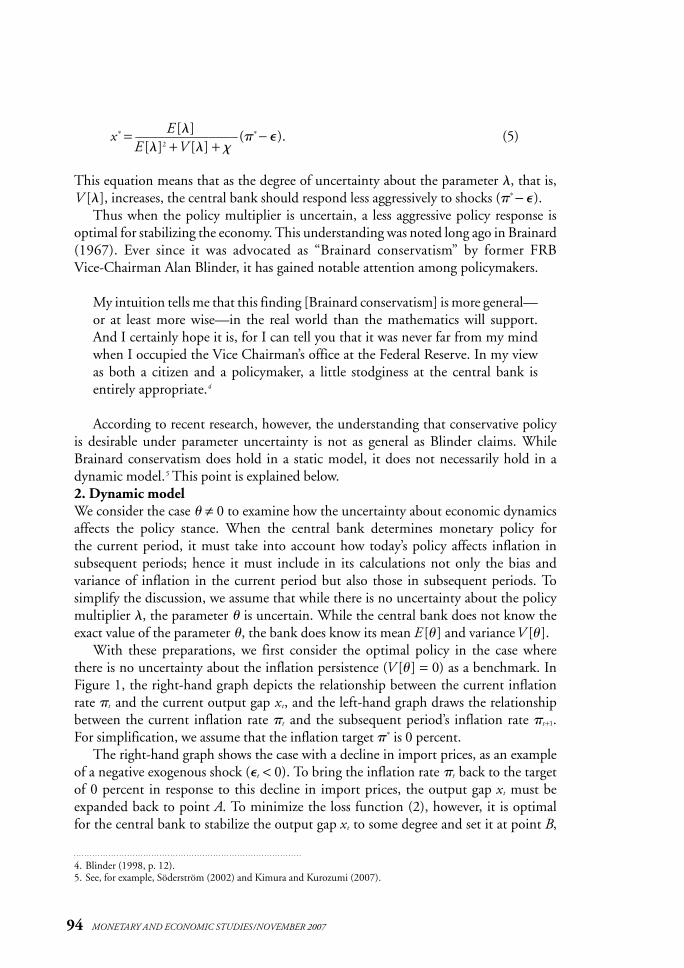
2. Dynamic model

We consider the case � ≠ 0 to examine how the uncertainty about economic dynamics

affects the policy stance. When the central bank determines monetary policy for

the current period, it must take into account how today’s policy affects inflation in

subsequent periods; hence it must include in its calculations not only the bias and

variance of inflation in the current period but also those in subsequent periods. To

simplify the discussion, we assume that while there is no uncertainty about the policy

multiplier �, the parameter � is uncertain. While the central bank does not know the

exact value of the parameter �, the bank does know its mean E [� ] and varianceV [� ].

With these preparations, we first consider the optimal policy in the case where

there is no uncertainty about the inflation persistence (V [� ] = 0) as a benchmark. In

Figure 1, the right-hand graph depicts the relationship between the current inflation

rate �t and the current output gap xt, and the left-hand graph draws the relationship

between the current inflation rate �t and the subsequent period’s inflation rate �t +1.

For simplification, we assume that the inflation target �* is 0 percent.

The right-hand graph shows the case with a decline in import prices, as an example

of a negative exogenous shock (�t < 0). To bring the inflation rate �t back to the target

of 0 percent in response to this decline in import prices, the output gap xt must be

expanded back to point A. To minimize the loss function (2), however, it is optimal

for the central bank to stabilize the output gap xt to some degree and set it at point B,


4. Blinder (1998, p. 12).5. See, for example, Söderström (2002) and Kimura and Kurozumi (2007).

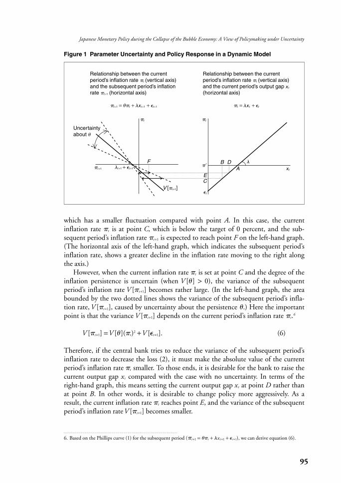
which has a smaller fluctuation compared with point A. In this case, the current

inflation rate �t is at point C, which is below the target of 0 percent, and the sub-

sequent period’s inflation rate �t +1 is expected to reach point F on the left-hand graph.

(The horizontal axis of the left-hand graph, which indicates the subsequent period’s

inflation rate, shows a greater decline in the inflation rate moving to the right along

the axis.)

However, when the current inflation rate �t is set at point C and the degree of the

inflation persistence is uncertain (when V [� ] > 0), the variance of the subsequent

period’s inflation rate V [�t +1] becomes rather large. (In the left-hand graph, the area

bounded by the two dotted lines shows the variance of the subsequent period’s infla-

tion rate,V [�t +1], caused by uncertainty about the persistence �.) Here the important

point is that the variance V [�t +1] depends on the current period’s inflation rate �t.6

V [�t +1] =V [� ](�t)2 +V [�t +1]. (6)

Therefore, if the central bank tries to reduce the variance of the subsequent period’s

inflation rate to decrease the loss (2), it must make the absolute value of the current

period’s inflation rate �t smaller. To those ends, it is desirable for the bank to raise the

current output gap xt compared with the case with no uncertainty. In terms of the

right-hand graph, this means setting the current output gap xt at point D rather than

at point B. In other words, it is desirable to change policy more aggressively. As a

result, the current inflation rate �t reaches point E, and the variance of the subsequent

period’s inflation rateV [�t +1] becomes smaller.

95


6. Based on the Phillips curve (1) for the subsequent period (�t +1 = ��t + �xt +1 + �t +1), we can derive equation (6).

Figure 1 Parameter Uncertainty and Policy Response in a Dynamic Model

AB

C

D

E

F

Uncertaintyabout

�t �t

�

�t +1

�

xt

�t

+1+1�t + �t�*

V [�t +1]

Relationship between the currentperiod’s inflation rate �t (vertical axis)and the subsequent period’s inflationrate �t +1 (horizontal axis)

�t +1 = ��t + �xt +1 + �t +1

Relationship between the currentperiod’s inflation rate �t (vertical axis)and the current period’s output gap xt

(horizontal axis)

�t = �xt + �t

This leads to the conclusion that it is desirable to implement aggressive rather than

conservative policy when there is uncertainty about economic dynamics.7 In short,

when there exists uncertainty about the inflation persistence, if the inflationary

(or deflationary) buds are not nipped today they may grow into greater inflation

(or deflation) tomorrow than expected. Excess inflation (or deflation) should be

nipped in the bud today to the greatest possible extent by implementing an aggressive

monetary policy.

Considering our analysis with both static and dynamic models, it is important to

know that the optimal policy response may differ depending on which parameter is

uncertain for the central bank.

B. Minimax Approach

Another approach to policy conduct under uncertainty is based on the idea that the

objective of the central bank is to minimize the maximum loss, which is referred to

as the “minimax approach” (or the “robust approach”). In this approach, instead of

holding a prior belief about the distribution of the uncertain parameters (�, �), the

central bank considers the conceivable range for them.

� ∈[�_, �_

], � ∈[�_, �_

]. (7)

The next step is to consider, within this range, which values of �, � will result in the

greatest loss, and to then select policies that will minimize that maximum loss. This

minimax approach can be expressed mathematically as follows.

�

Min Max Et�� j[(�t +j − �*)2 + (xt +j)2]. (8){xt} {�,�} j =0

s.t. �t = ��t −1 + �xt + �t

The following subsections examine whether the central bank that adopts the

minimax approach should implement more conservative or more aggressive policy

under uncertainty.

1. Static model

To simplify the discussion, we once again consider the static model (� = 0) and assume

that the parameter � is uncertain. We consider the following policy response function

in which the policy variable x responds to the difference between the inflation target

and the exogenous shock (�* − �).


7. This conclusion is derived under the dynamic model because the influence of exogenous shocks on the economy isnot completely offset at the current period and can be carried over to subsequent periods. In fact, as explained in thispaper, because the price shock that shifts the Phillips curve up or down leads to a trade-off between the inflation ratestabilization and the output gap stabilization, the shock effect is carried over to the subsequent period. On the otherhand, when there is a demand shock that shifts the IS curve, theoretically its influence can be completely offset bycontrolling interest rates. However, this only holds true when the central bank has complete information on thedemand shock and can change interest rates without any cost. In reality, central banks have imperfect informationand must give some consideration to interest rate smoothing in their policy conduct, so they cannot completely offset the influence of demand shocks on the inflation rate, and this influence is carried over to the subsequentperiod. Therefore, the considerations in this paper hold regardless of the nature of the shock. For details, see Kimuraand Kurozumi (2007).

x =h (�* − �). (9)

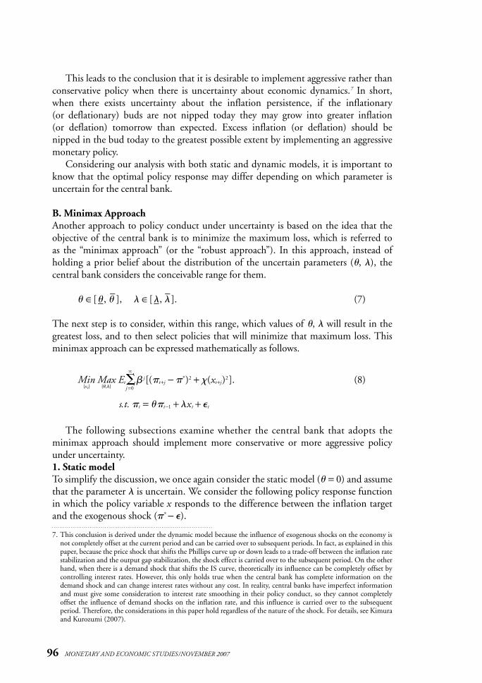
In equation (9), the coefficient h denotes the degree of policy response. Figure 2 shows

how the central bank’s loss (3) shifts with changes in the policy response h under a

given parameter �.8

Here let us assume that the true value of the parameter � is 1.5. The central

bank does not know this true value, and it considers the range for � of between 1.0

and 2.0. If policy is determined based on the minimax approach, the central bank

implements its policy assuming that � = 1.0 because that leads to the maximum

loss within that conceivable range for �. The reason why the maximum loss occurs in

the case of � = 1.0 is that the central bank must greatly change the output gap x to

stabilize the inflation rate � when the value of �, that is, the slope of the Phillips

curve, is small. And when � is small, the price stability will not be achieved unless the

central bank sets a higher value for h and implements an aggressive policy. In this

manner, when there is uncertainty about the parameter �, it is desirable for the central

bank to implement more aggressive monetary policy than under the case in which the

central bank knows the true value of �.9

97


8. Figure 2 shows the loss in the case of = 1.9. This conclusion is consistent with what the previous literature on the minimax approach suggests. See Giannoni

(2002, 2006), Hansen and Sargent (2003), Sargent (1999), Stock (1999), and Onatski and Stock (2002).

Figure 2 Minimax Approach

Loss

0.20 0.25 0.30 0.35 0.40 0.45 0.50 0.55Policy response: h

0.15

0.25

0.35

0.45

0.55

0.65

0.75

0.85 � = 0.5

� = 1.0

� = 1.5

� = 2.0

Note: • indicates the point where the loss is minimized for each parameter �.

However, the minimax approach does not necessarily always support aggressive

policy. For example, if the central bank assumes the conceivable range for � as

0.5 ≤ � ≤ 2.0, the bank will find a rather more conservative policy, � = 0.5, to be desir-

able.10 Thus, it is important to note that monetary policy stance under the minimax

approach may be dependent on the degree of the uncertainty, that is, the conceivable

range of the parameter.

2. Dynamic model

In recent years, research has also been advancing on the minimax approach using

the dynamic model (� ≠ 0). While the details are omitted here, the loss under the

dynamic model is at the highest level when the value of � is high, that is, in the case

with high inflation persistence. With high inflation persistence, control of inflation

via monetary policy becomes difficult because the upward pressure on inflation does

not easily subside once a rise in the inflation rate gains strength. For that reason, the

generally accepted view of the minimax approach is that the central bank should

pursue an aggressive policy on the assumption of high inflation persistence to minimize

the maximum loss.11

Although monetary policy based on the minimax approach may depend upon

the degree of uncertainty, that is, the conceivable range of uncertain parameters,

the above examples suggest that it is important to consider potentially large losses,

which might occur in the future, in the conduct of monetary policy. In fact, the former

FRB Chairman Alan Greenspan referred to his own policy conduct style as the “risk

management approach,” which can be interpreted as the one reflecting the minimax

approach perspective (see Greenspan [2003]).

III. Model

A. The JEM and the Policy Rule

The JEM used in our analyses is a large-scale dynamic general equilibrium model

comprising 219 equations, but one may consider its essence as being summarized

in the two equations: the Phillips curve and the IS curve. These are both hybrid

equations combining forward-looking and backward-looking expectations of the

private sector (see Fujiwara et al. [2005]).

�t = ��t −1 + (1 − � )Et [�t +1] + �(yt − y*t ) +�t . (10)

yt − y*t = �(yt −1 – y*

t −1) + (1 − �)Et [yt +1 − y*t +1] − � (it −Et [�t +1] − r*) + t.

(11)


10. When the slope of the Phillips curve � is extremely small, the change in the output gap, which must be sacrificedfor inflation stabilization, is extremely large and the central bank’s loss increases very significantly. In other words,when extremely poor policy efficiency is assumed as the worst case, a cautious policy response is desirable becausean aggressive policy only overshoots the output gap but does not contribute all that much to inflation stabilization.

11. See, for example, Angeloni, Coenen, and Smets (2003).

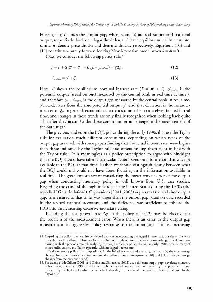
Here, yt − y*t denotes the output gap, where yt and y*

t are real output and potential

output, respectively, both on a logarithmic basis. r* is the equilibrium real interest rate.

�t and t denote price shocks and demand shocks, respectively. Equations (10) and

(11) constitute a purely forward-looking New Keynesian model when � = � = 0.

Next, we consider the following policy rule.12

it = i * +�(�t − �*) +�(yt − y*t|realtime) +��yt. (12)

y*t|realtime = y*

t + �t. (13)

Here, i * shows the equilibrium nominal interest rate (i * = �* + r*). y*t|realtime is the

potential output (trend output) measured by the central bank in real time at time t,

and therefore yt − y*t|realtime is the output gap measured by the central bank in real time.

y*t|realtime deviates from the true potential output y*

t , and that deviation is the measure-

ment error �t. In general, economic data trends cannot be accurately estimated in real

time, and changes in those trends are only finally recognized when looking back quite

a bit after they occur. Under these conditions, errors emerge in the measurement of

the output gap.

The previous studies on the BOJ’s policy during the early 1990s that use the Taylor

rule for evaluation reach different conclusions, depending on which types of the

output gap are used, with some papers finding that the actual interest rates were higher

than those indicated by the Taylor rule and others finding them right in line with

the Taylor rule.13 It is meaningless as a policy prescription to argue with hindsight

that the BOJ should have taken a particular action based on information that was not

available to the BOJ at that time. Rather, we should distinguish clearly between what

the BOJ could and could not have done, focusing on the information available in

real time. The great importance of considering the measurement error of the output

gap when conducting monetary policy is well known from U.S. case studies.

Regarding the cause of the high inflation in the United States during the 1970s (the

so-called “Great Inflation”), Orphanides (2001, 2003) argues that the real-time output

gap, as measured at that time, was larger than the output gap based on data recorded

in the revised national accounts, and the difference was sufficient to mislead the

FRB into implementing excessive monetary easing.

Including the real growth rate �yt in the policy rule (12) may be effective for

the problem of the measurement error. When there is an error in the output gap

measurement, an aggressive policy response to the output gap—that is, increasing

99


12. Regarding the policy rule, we also conducted analyses incorporating the lagged interest rate, but the results werenot substantially different. Here, we focus on the policy rule without interest rate smoothing to facilitate com-parison with the previous research analyzing the BOJ’s monetary policy during the early 1990s, because many ofthose studies employ the Taylor-type rules without lagged interest rate.

In the monetary policy rule in equation (12), the inflation rate �t and the real growth rate �y show percentagechanges from the previous year (in contrast, the inflation rate �t in equations [10] and [11] shows percentagechanges from the previous period).

13. For example, McCallum (2001) and Okina and Shiratsuka (2002) use a different output gap to evaluate monetarypolicy during the early 1990s. The former finds that actual interest rate levels were high compared with those indicated by the Taylor rule, while the latter finds that they were essentially consistent with those indicated by theTaylor rule.

the value of � in equation (12)—results in unnecessary interest rate fluctuations

corresponding to the measurement error �t, which may cause economic instability.

One approach to averting this problem is to target the real growth rate �yt instead

of the output gap.14

B. Parameter Uncertainty Faced by the BOJ

Fujiwara et al. (2005) shows that the impulse response of the JEM to various types of

shocks is roughly the same as the VAR impulse response based on the sample period

1983–95. Hence, the set of parameters of equations (10) and (11), which are the basic

JEM equations, depict adequately the structure of the Japanese economy during that

period. On a real-time basis, however, the BOJ did not fully understand the parameters

of the economic structure at that time, and in that sense it is appropriate to believe

that the BOJ faced parameter uncertainty.

In this paper, we analyze the uncertainty about the following four parameters:

(1) policy multiplier; (2) inflation persistence; (3) price shock persistence; and (4) demand

shock persistence.

1. Uncertainty about the policy multiplier

In the IS curve (11), the parameter of the real interest rate gap, �, can be interpreted

as the policy multiplier.

yt − y*t = �(yt −1 – y*

t −1) + (1 − �)Et [yt +1 − y*t +1] − � (it −Et [�t +1] − r*) + t.

(11)

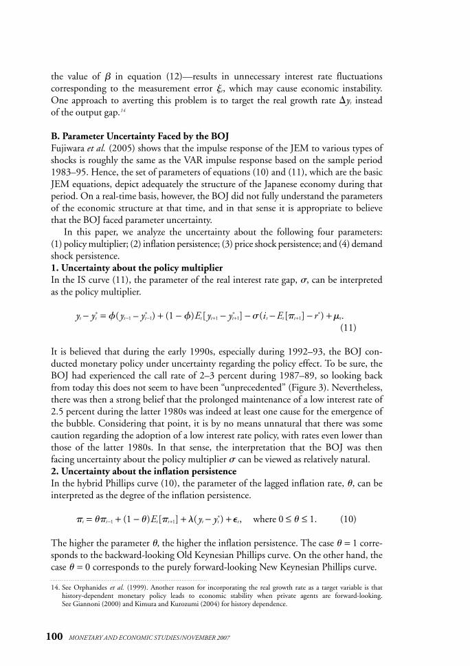
It is believed that during the early 1990s, especially during 1992–93, the BOJ con-

ducted monetary policy under uncertainty regarding the policy effect. To be sure, the

BOJ had experienced the call rate of 2–3 percent during 1987–89, so looking back

from today this does not seem to have been “unprecedented” (Figure 3). Nevertheless,

there was then a strong belief that the prolonged maintenance of a low interest rate of

2.5 percent during the latter 1980s was indeed at least one cause for the emergence of

the bubble. Considering that point, it is by no means unnatural that there was some

caution regarding the adoption of a low interest rate policy, with rates even lower than

those of the latter 1980s. In that sense, the interpretation that the BOJ was then

facing uncertainty about the policy multiplier � can be viewed as relatively natural.

2. Uncertainty about the inflation persistence

In the hybrid Phillips curve (10), the parameter of the lagged inflation rate, �, can be

interpreted as the degree of the inflation persistence.

�t = ��t −1 + (1 − � )Et [�t +1] + �(yt − y*t ) +�t , where 0 ≤ � ≤ 1. (10)

The higher the parameter �, the higher the inflation persistence. The case � = 1 corre-

sponds to the backward-looking Old Keynesian Phillips curve. On the other hand, the

case � = 0 corresponds to the purely forward-looking New Keynesian Phillips curve.


14. See Orphanides et al. (1999). Another reason for incorporating the real growth rate as a target variable is that history-dependent monetary policy leads to economic stability when private agents are forward-looking. See Giannoni (2000) and Kimura and Kurozumi (2004) for history dependence.

Even now that a substantial volume of empirical research on hybrid Phillips curves

has accumulated, academics have still not reached a consensus regarding the estima-

tion results of the parameter �.15 For that reason, it is appropriate to consider that not

only the BOJ but all central banks are constantly facing uncertainty regarding the

inflation persistence. In addition, it is important to note that during the early 1990s

there was no knowledge about the hybrid Phillips curves expressed by equation (10),

since research had not been conducted on the New Keynesian Phillips curve.16 In that

sense, rather than saying that the BOJ faced uncertainty about the parameter � at that

time, it may be more accurate to say that there was uncertainty about the overall form

of the structural equation.

The reduced form of the hybrid Phillips curve (10) can be expressed as equation (14).17

�t = ��t −1 + �(yt −1 − y*t −1) + �t. (14)

In the early 1990s, there was a debate regarding the estimate of the parameter � in

equation (14) inside the BOJ, while no consensus had been gained there regarding its

estimated value.18 Given the relation whereby reduced-form parameter � in equation

(14) increases as the structural parameter � in equation (10) increases, a contemporary

interpretation for the fact that there was no consensus inside the BOJ regarding the

101


Figure 3 Policy Interest Rates

0

1

2

3

4

5

6

7

8

9

1985 86 87 88 89 90 91 92 93 94 95 96CY

Annual rate, percent

The lowest level of the discount rate beforethe collapse of the bubble economy (2.5 percent)

Official discount rateCall rate (overnight, uncollateralized)

Source: Bank of Japan.

15. For details, see Kimura and Kurozumi (2007). Regarding the estimation results of Japanese Phillips curves, seeKimura and Kurozumi (2004).

16. The New Keynesian Phillips curve became widely discussed in academic circles following the publication ofRoberts (1995).

17. For details, see Rudebusch (2005). 18. See, for example, Tanaka and Kimura (1998) and Watanabe (1997). The former supports the NAIRU hypothesis

(� = 1), while the latter denies it. Both of these papers were published in the latter 1990s, but the research forboth had already begun in the early 1990s.

estimation of the parameter � would be that at that time the BOJ had no certain

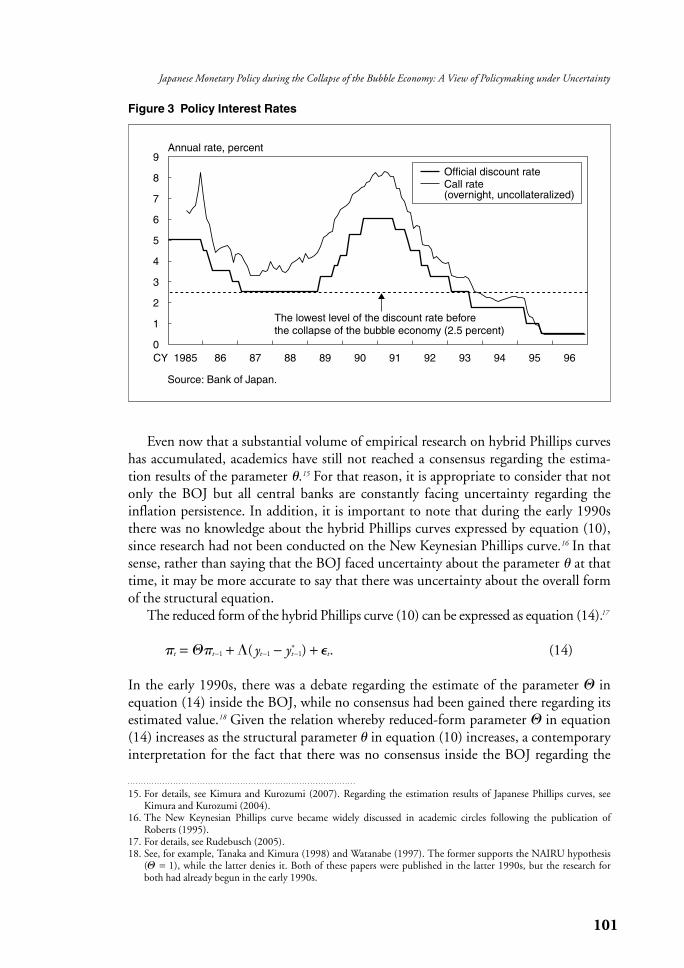
knowledge about the hybrid Phillips curve parameter �. (See Figure 4 for changes in

the inflation rate.)

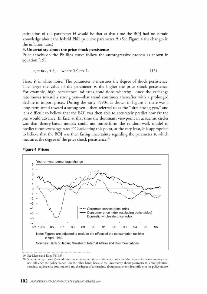
3. Uncertainty about the price shock persistence

Price shocks on the Phillips curve follow the autoregressive process as shown in

equation (15).

�t = ��t −1 + �t̂ , where 0 ≤ � < 1. (15)

Here, �t̂ is white noise. The parameter � measures the degree of shock persistence.

The larger the value of the parameter �, the higher the price shock persistence.

For example, high persistence indicates conditions whereby—once the exchange

rate moves toward a strong yen—that trend continues thereafter with a prolonged

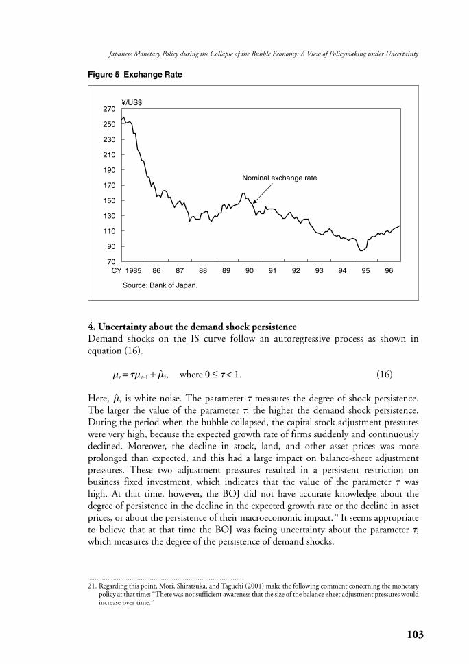
decline in import prices. During the early 1990s, as shown in Figure 5, there was a

long-term trend toward a strong yen—then referred to as the “ultra-strong yen,” and

it is difficult to believe that the BOJ was then able to accurately predict how far the

yen would advance. In fact, at that time the dominant viewpoint in academic circles

was that theory-based models could not outperform the random-walk model to

predict future exchange rates.19 Considering this point, at the very least, it is appropriate

to believe that the BOJ was then facing uncertainty regarding the parameter �, which

measures the degree of the price shock persistence.20


Figure 4 Prices

–7

–6

–5

–4

–3

–2

–1

0

1

2

3

4

5

1985 86 87 88 89 90 91 92 93 94 95 96CY

Year-on-year percentage change

Corporate service price indexConsumer price index (excluding perishables)Domestic wholesale price index

Note: Figures are adjusted to exclude the effects of the consumption tax hike in April 1989.

Sources: Bank of Japan; Ministry of Internal Affairs and Communications.

19. See Meese and Rogoff (1983).20. Since �t̂ in equation (15) is additive uncertainty, certainty equivalence holds and the degree of this uncertainty does

not influence the policy stance. On the other hand, because the uncertainty about parameter � is multiplicative, certainty equivalence does not hold and the degree of uncertainty about parameter � does influence the policy stance.

4. Uncertainty about the demand shock persistence

Demand shocks on the IS curve follow an autoregressive process as shown in

equation (16).

t = � t–1 + ̂t, where 0 ≤ � < 1. (16)

Here, ̂t is white noise. The parameter � measures the degree of shock persistence.

The larger the value of the parameter �, the higher the demand shock persistence.

During the period when the bubble collapsed, the capital stock adjustment pressures

were very high, because the expected growth rate of firms suddenly and continuously

declined. Moreover, the decline in stock, land, and other asset prices was more

prolonged than expected, and this had a large impact on balance-sheet adjustment

pressures. These two adjustment pressures resulted in a persistent restriction on

business fixed investment, which indicates that the value of the parameter � was

high. At that time, however, the BOJ did not have accurate knowledge about the

degree of persistence in the decline in the expected growth rate or the decline in asset

prices, or about the persistence of their macroeconomic impact.21 It seems appropriate

to believe that at that time the BOJ was facing uncertainty about the parameter �,

which measures the degree of the persistence of demand shocks.

103


21. Regarding this point, Mori, Shiratsuka, and Taguchi (2001) make the following comment concerning the monetarypolicy at that time: “There was not sufficient awareness that the size of the balance-sheet adjustment pressures wouldincrease over time.”

Figure 5 Exchange Rate

70

90

110

130

150

170

190

210

230

250

270

1985 86 87 88 89 90 91 92 93 94 95 96

Nominal exchange rate

CY

¥/US$


C. Policy Evaluation Criteria

In the limit when the discount factor approaches unity, in other words, �→1, the

central bank’s loss function (2) is proportional to the following weighted sum of

the variances.22

Var [�t − �*] + Var [yt − y*t ]. (17)

It is desirable for the central bank to set the policy rule to minimize the loss given

by equation (17). In the following, we discuss how the central bank should set the

relative weight on the output gap stabilization .

1. New Keynesian economics and price stability

The new Keynesian economics has theoretically derived the value of to reflect

social welfare losses, which depend on the variance of the output gap and on the

magnitude of the price dispersion across firms.23 There are two major specifications of

firms’ pricing behavior that the New Keynesian economics suggest: random-duration

contracts called “Calvo-style” (Calvo [1983]) and fixed-duration contracts called

“Taylor-style” (Taylor [1980]). Under the specification of random-duration contracts,

some contracts remain unchanged over long stretches of time, even if the average

contract duration is relatively short; thus, fluctuations in aggregate inflation tend to

have highly persistent effects on relative price dispersion, so that the welfare cost of

the inflation volatility is roughly two orders of magnitude greater than that of the

output gap volatility (see Rotemberg and Woodford [1997]).

In contrast, fixed-duration contracts induce much less intrinsic persistence of the

relative price dispersion, and hence imply that the welfare cost of inflation volatility is

much smaller, and in fact roughly comparable in magnitude to that of the output gap

volatility. As shown in Erceg and Levin (2002), using an appropriate parameter set

with Taylor-style contracts, the relative weight on the output gap stabilization is

around unity.

2. Weight on the price stability in Japan

In Japan, there is a tendency toward “synchronized price setting” whereby firms revise

their prices simultaneously at specific times of the year, typically in April and

October.24 So the actual welfare losses due to the relative price dispersion cannot be

large to the extent posited by Taylor (1980). For this reason, > 1 may be a good

approximation of social welfare in Japan.

Regarding the welfare cost of the inflation volatility, it is also necessary to consider

the fact that the CPI inflation rate remained in a range between 0 percent and

2 percent from the 1980s through the early 1990s, excluding the brief period 1990–91.

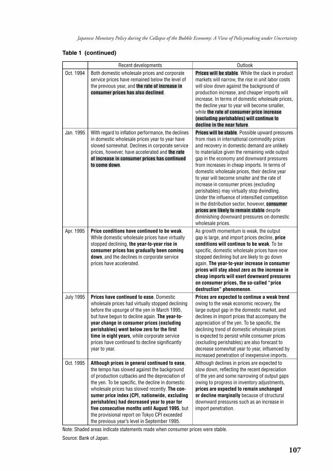
According to the “Quarterly Economic Outlook,” the BOJ judged that prices were

stable when the CPI inflation rate remained within that range (Table 1 and Figure 6).


22. Note that xt in equation (2) is the output gap(yt − y*t ).

23. See the survey in Kimura, Fujiwara, and Kurozumi (2005).24. See Saita et al. (2006) regarding the Japanese price revisions.

105


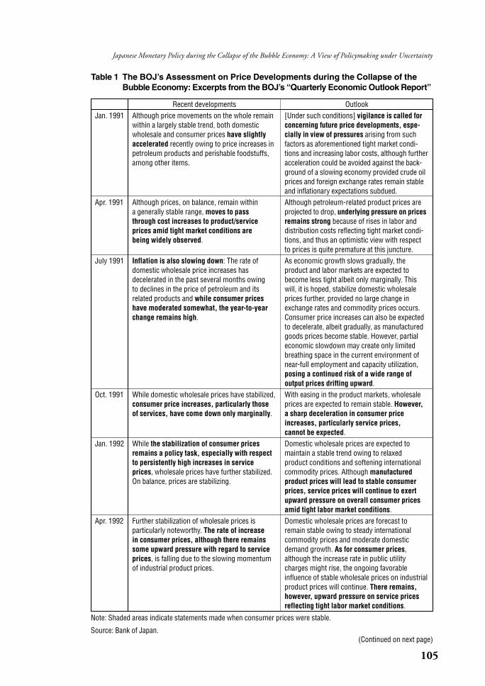
Table 1 The BOJ’s Assessment on Price Developments during the Collapse of theBubble Economy: Excerpts from the BOJ’s “Quarterly Economic Outlook Report”

Jan. 1991

Apr. 1991

July 1991

Oct. 1991

Jan. 1992

Apr. 1992

Recent developmentsAlthough price movements on the whole remainwithin a largely stable trend, both domesticwholesale and consumer prices have slightlyaccelerated recently owing to price increases inpetroleum products and perishable foodstuffs,among other items.

Although prices, on balance, remain within a generally stable range, moves to pass through cost increases to product/service prices amid tight market conditions are being widely observed.

Inflation is also slowing down: The rate ofdomestic wholesale price increases has decelerated in the past several months owing to declines in the price of petroleum and itsrelated products and while consumer priceshave moderated somewhat, the year-to-yearchange remains high.

While domestic wholesale prices have stabilized,consumer price increases, particularly those of services, have come down only marginally.

While the stabilization of consumer pricesremains a policy task, especially with respectto persistently high increases in service prices, wholesale prices have further stabilized.On balance, prices are stabilizing.

Further stabilization of wholesale prices is particularly noteworthy. The rate of increase in consumer prices, although there remainssome upward pressure with regard to serviceprices, is falling due to the slowing momentumof industrial product prices.

Outlook[Under such conditions] vigilance is called forconcerning future price developments, espe-cially in view of pressures arising from suchfactors as aforementioned tight market condi-tions and increasing labor costs, although furtheracceleration could be avoided against the back-ground of a slowing economy provided crude oilprices and foreign exchange rates remain stableand inflationary expectations subdued.Although petroleum-related product prices areprojected to drop, underlying pressure on pricesremains strong because of rises in labor anddistribution costs reflecting tight market condi-tions, and thus an optimistic view with respect to prices is quite premature at this juncture.As economic growth slows gradually, the product and labor markets are expected tobecome less tight albeit only marginally. Thiswill, it is hoped, stabilize domestic wholesaleprices further, provided no large change inexchange rates and commodity prices occurs.Consumer price increases can also be expectedto decelerate, albeit gradually, as manufacturedgoods prices become stable. However, partialeconomic slowdown may create only limitedbreathing space in the current environment ofnear-full employment and capacity utilization,posing a continued risk of a wide range of output prices drifting upward.With easing in the product markets, wholesaleprices are expected to remain stable. However, a sharp deceleration in consumer priceincreases, particularly service prices, cannot be expected.Domestic wholesale prices are expected to maintain a stable trend owing to relaxed product conditions and softening internationalcommodity prices. Although manufacturedproduct prices will lead to stable consumerprices, service prices will continue to exertupward pressure on overall consumer pricesamid tight labor market conditions.Domestic wholesale prices are forecast toremain stable owing to steady international commodity prices and moderate domesticdemand growth. As for consumer prices,although the increase rate in public utilitycharges might rise, the ongoing favorable influence of stable wholesale prices on industrialproduct prices will continue. There remains,however, upward pressure on service pricesreflecting tight labor market conditions.

Note: Shaded areas indicate statements made when consumer prices were stable.

Source: Bank of Japan.(Continued on next page)


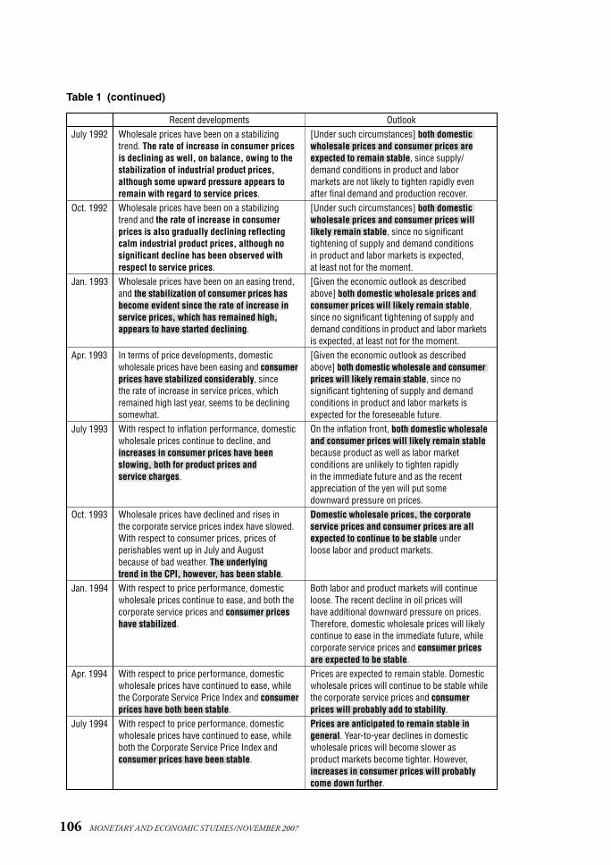
Table 1 (continued)

July 1992

Oct. 1992

Jan. 1993

Apr. 1993

July 1993

Oct. 1993

Jan. 1994

Apr. 1994

July 1994

Recent developments Outlook[Under such circumstances] both domesticwholesale prices and consumer prices areexpected to remain stable, since supply/demand conditions in product and labor markets are not likely to tighten rapidly evenafter final demand and production recover.[Under such circumstances] both domesticwholesale prices and consumer prices willlikely remain stable, since no significant tightening of supply and demand conditions in product and labor markets is expected, at least not for the moment.[Given the economic outlook as describedabove] both domestic wholesale prices andconsumer prices will likely remain stable,since no significant tightening of supply anddemand conditions in product and labor marketsis expected, at least not for the moment.[Given the economic outlook as described above] both domestic wholesale and consumerprices will likely remain stable, since no significant tightening of supply and demand conditions in product and labor markets isexpected for the foreseeable future.On the inflation front, both domestic wholesaleand consumer prices will likely remain stablebecause product as well as labor market conditions are unlikely to tighten rapidly in the immediate future and as the recent appreciation of the yen will put some downward pressure on prices.Domestic wholesale prices, the corporate service prices and consumer prices are allexpected to continue to be stable under loose labor and product markets.

Both labor and product markets will continueloose. The recent decline in oil prices will have additional downward pressure on prices.Therefore, domestic wholesale prices will likelycontinue to ease in the immediate future, whilecorporate service prices and consumer pricesare expected to be stable.Prices are expected to remain stable. Domesticwholesale prices will continue to be stable whilethe corporate service prices and consumerprices will probably add to stability.Prices are anticipated to remain stable in general. Year-to-year declines in domesticwholesale prices will become slower as product markets become tighter. However,increases in consumer prices will probablycome down further.

Wholesale prices have been on a stabilizingtrend. The rate of increase in consumer pricesis declining as well, on balance, owing to thestabilization of industrial product prices,although some upward pressure appears toremain with regard to service prices.Wholesale prices have been on a stabilizingtrend and the rate of increase in consumerprices is also gradually declining reflectingcalm industrial product prices, although nosignificant decline has been observed withrespect to service prices.Wholesale prices have been on an easing trend,and the stabilization of consumer prices hasbecome evident since the rate of increase inservice prices, which has remained high,appears to have started declining.

In terms of price developments, domesticwholesale prices have been easing and consumerprices have stabilized considerably, since the rate of increase in service prices, whichremained high last year, seems to be decliningsomewhat.With respect to inflation performance, domesticwholesale prices continue to decline, andincreases in consumer prices have been slowing, both for product prices and service charges.

Wholesale prices have declined and rises in the corporate service prices index have slowed.With respect to consumer prices, prices of perishables went up in July and August because of bad weather. The underlying trend in the CPI, however, has been stable.With respect to price performance, domesticwholesale prices continue to ease, and both thecorporate service prices and consumer priceshave stabilized.

With respect to price performance, domesticwholesale prices have continued to ease, whilethe Corporate Service Price Index and consumerprices have both been stable.With respect to price performance, domesticwholesale prices have continued to ease, whileboth the Corporate Service Price Index and consumer prices have been stable.

107


Table 1 (continued)

Oct. 1994

Jan. 1995

Apr. 1995

July 1995

Oct. 1995

Recent developments OutlookPrices will be stable. While the slack in productmarkets will narrow, the rise in unit labor costswill slow down against the background of production increase, and cheaper imports willincrease. In terms of domestic wholesale prices,the decline year to year will become smaller,while the rate of consumer price increase(excluding perishables) will continue todecline in the near future.Prices will be stable. Possible upward pressuresfrom rises in international commodity prices and recovery in domestic demand are unlikely to materialize given the remaining wide outputgap in the economy and downward pressuresfrom increases in cheap imports. In terms ofdomestic wholesale prices, their decline year to year will become smaller and the rate ofincrease in consumer prices (excluding perishables) may virtually stop dwindling. Under the influence of intensified competition in the distribution sector, however, consumerprices are likely to remain stable despitediminishing downward pressures on domesticwholesale prices.As growth momentum is weak, the output gap is large, and import prices decline, priceconditions will continue to be weak. To be specific, domestic wholesale prices have nowstopped declining but are likely to go downagain. The year-to-year increase in consumerprices will stay about zero as the increase incheap imports will exert downward pressureson consumer prices, the so-called “pricedestruction” phenomenon.Prices are expected to continue a weak trendowing to the weak economic recovery, the large output gap in the domestic market, anddeclines in import prices that accompany theappreciation of the yen. To be specific, thedeclining trend of domestic wholesale prices is expected to persist while consumer prices(excluding perishables) are also forecast todecrease somewhat year to year, influenced byincreased penetration of inexpensive imports.Although declines in prices are expected to slow down, reflecting the recent depreciation of the yen and some narrowing of output gapsowing to progress in inventory adjustments,prices are expected to remain unchanged or decline marginally because of structuraldownward pressures such as an increase inimport penetration.

Both domestic wholesale prices and corporateservice prices have remained below the level ofthe previous year, and the rate of increase inconsumer prices has also declined.

With regard to inflation performance, the declinesin domestic wholesale prices year to year haveslowed somewhat. Declines in corporate serviceprices, however, have accelerated and the rate of increase in consumer prices has continuedto come down.

Price conditions have continued to be weak.While domestic wholesale prices have virtuallystopped declining, the year-to-year rise in consumer prices has gradually been comingdown, and the declines in corporate serviceprices have accelerated.

Prices have continued to ease. Domesticwholesale prices had virtually stopped decliningbefore the upsurge of the yen in March 1995, but have begun to decline again. The year-to-year change in consumer prices (excludingperishables) went below zero for the first time in eight years, while corporate serviceprices have continued to decline significantlyyear to year.

Although prices in general continued to ease,the tempo has slowed against the background of production cutbacks and the depreciation ofthe yen. To be specific, the decline in domesticwholesale prices has slowed recently. The con-sumer price index (CPI, nationwide, excludingperishables) had decreased year to year forfive consecutive months until August 1995, butthe provisional report on Tokyo CPI exceeded the previous year’s level in September 1995.

Note: Shaded areas indicate statements made when consumer prices were stable.


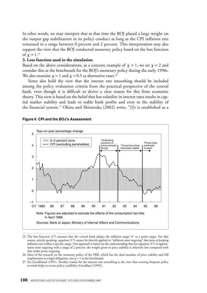
In other words, we may interpret that at that time the BOJ placed a large weight on

the output gap stabilization in its policy conduct as long as the CPI inflation rate

remained in a range between 0 percent and 2 percent. This interpretation may also

support the view that the BOJ conducted monetary policy based on the loss function

of > 1.25

3. Loss function used in the simulation

Based on the above considerations, as a concrete example of > 1, we set = 2 and

consider this as the benchmark for the BOJ’s monetary policy during the early 1990s.

We also examine = 1 and = 0.5 as alternative cases.26

Some also hold the view that the interest rate smoothing should be included

among the policy evaluation criteria from the practical perspective of the central

bank, even though it is difficult to derive a clear reason for this from economic

theory. This view is based on the belief that less volatility in interest rates results in cap-

ital market stability and leads to stable bank profits and even to the stability of

the financial system.27 Okina and Shiratsuka (2002) write, “[I]t is established as a


25. The loss function (17) assumes that the central bank adopts the inflation target �* as a point target. For that reason, strictly speaking, equation (17) cannot be directly applied to “inflation zone targeting” that aims at keepinginflation rate within a specific range. Our approach is based on the understanding that for equation (17) to approx-imate zone targeting with a range of 2 percent, the weight given to price stability is relatively low compared withthat under point targeting.

26. Most of the research on the monetary policy of the FRB, which has the dual mandate of price stability and fullemployment as a legal obligation, sets = 1 as the benchmark.

27. See Goodfriend (1991). Another reason for the interest rate smoothing is the view that averting frequent policyreversals helps to secure policy credibility (Goodhart [1999]).

Figure 6 CPI and the BOJ’s Assessment

–1

0

1

2

3

4

5Year-on-year percentage change

1985 86 87 88 89 90 91 92 93 94 95 96CY

0–2 percent zoneCPI (excluding perishables)

“Underlying pressure on prices remains strong”

“Consumer prices have been stable”

“Prices have continued to ease”

Note: Figures are adjusted to exclude the effects of the consumption tax hike in April 1989.

Sources: Bank of Japan; Ministry of Internal Affairs and Communications.

practice of central banks worldwide, including that in Japan, to avoid unexpected

large changes in interest rates. Thus, it is undeniable that ignoring such practices

might trigger financial system turbulence.” In this paper, considering this practical

perspective, we adopt the following loss function, which incorporates the interest rate

smoothing, for the policy evaluation criteria.

Var [�t − �*] + Var [yt − y*t ] + �Var [�it ]. (18)

Specifically, in line with some previous studies, we set � = 0.5 as a benchmark, and

� = 0 as an alternative case.28

We now advance the analyses with the understanding that the BOJ implemented

policy in the early 1990s to minimize the loss function under the combination = 2

and � = 0.5.

IV. Results of the Analyses

A. Estimation Results of the Policy Rule

We estimate the policy rule (12) to evaluate the BOJ’s actual policy conduct.

it = �(�t ) + �(yt − y*t|realtime) + ��yt + c, (12)

where the constant term c = i * − ��*.

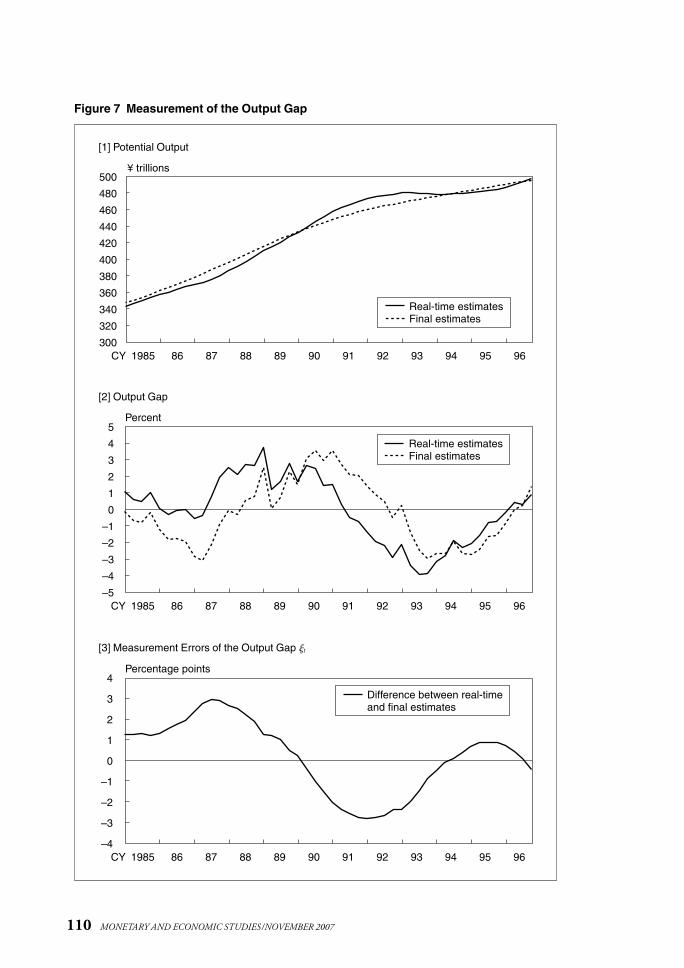
Two types of estimates for the potential output and the output gap used for the

estimation are shown in Figure 7. Based on the production function approach, we

estimate total factor productivity by applying a Hodrick-Prescott (HP) filter to the

Solow residual. The “final estimates” for potential output in the figure are the estimates

applying the HP filter to the Solow residual up to 2005. The “real-time estimate”

for potential output at a certain quarter is obtained by applying the filter to the

Solow residual up to that quarter. For example, the “real-time estimate” for the output

gap in 1991/Q1 means the output gap measured using the data up until 1991/Q1.

The retroactive revision in potential output from real-time estimates to final estimates

is the measurement error �t in equation (13). In practice, the real-time estimates will

be greatly revised retroactively by applying the HP filter again after adding subsequent

economic data. Thus, it is difficult to accurately estimate the economic trend in

real time, particularly near the end of the history. In reality, the standard deviation of

the measurement error during 1986–95 is 1.9 percent. Therefore, it is inappropriate

to ignore the existence of measurement error in potential output in estimating the

policy rule.29

Estimation results of the policy rule (12) are as follows.30

109


28. Some previous studies analyzing FRB monetary policy adopt the settings = 1 and � = 0.5; see, for example,Rudebusch (2001) and Williams (2004).

29. Incidentally, according to Orphanides et al. (1999), the standard deviation of the output gap measurement error inthe United States was 1.8 percent during 1980–94 and 3.8 percent during 1966–94.

30. The estimation is based on ordinary least squares (OLS), but essentially the same results were obtained when theestimation was conducted using the instrument variable method.


Figure 7 Measurement of the Output Gap

300

320

340

360

380

400

420

440

460

480

500

1985 86 87 88 89 90 91 92 93 94 95 96CY

¥ trillions

Real-time estimatesFinal estimates

[1] Potential Output

1985 86 87 88 89 90 91 92 93 94 95 96CY–5

–4

–3

–2

–1

0

1

2

3

4

5Percent

Real-time estimatesFinal estimates

[2] Output Gap

1985 86 87 88 89 90 91 92 93 94 95 96CY–4

–3

–2

–1

0

1

2

3

4Percentage points

Difference between real-time and final estimates

[3] Measurement Errors of the Output Gap �t

it = 1.58�t + 0.51(yt − y*t|realtime) − 0.10�yt + 2.78, R

–2 = 0.83, S.E. = 0.83.

(11.63) (3.44) (–0.75) (5.49) (19)

The t values are in parentheses. The sample period is from 1986/Q1 through 1995/Q4.

Since the coefficient of the real growth rate �yt is not statistically significant, we

estimate the policy rule without �yt.

it = 1.60�t + 0.41(yt − y*t|realtime) + 2.43, R

–2 = 0.84, S.E. = 0.81.

(12.32) (7.05) (11.22) (20)

As the estimation results (�, � ) = (1.6, 0.4) are very close to the original Taylor rule

(�, � ) = (1.5, 0.5), the actual policy interest rates were essentially determined in line

with the Taylor rule.31 Hereafter, we assume that the BOJ’s monetary policy during

the early 1990s can be depicted by the policy rule with (�, �, � ) = (1.6, 0.4, 0.0).

Moreover, taking into account the estimation error of the policy rule, it seems more

appropriate to refer to confidence intervals than to specific values of � and �. This

point is considered as needed in the following analyses.

We also find that when the final estimates (yt − y*t ) rather than the real-time

estimates (yt − y*t|realtime) are used for the output gap, Taylor’s principle (� > 1) is not

satisfied, and the coefficient of determination R–

2 worsens considerably.

it = 0.93�t + 0.46(yt − y*t ) + 3.33, R

–2 = 0.73, S.E. = 1.04.

(3.94) (3.63) (8.33) (21)

Thus, as is clear from the difference in the estimation results under equations (20) and

(21), it is important to consider the measurement error of the output gap in the policy

evaluation.

B. Simulation Results without Parameter Uncertainty

To examine how parameter uncertainty affects monetary policy implementation, we

first derive the optimal policy when there is no uncertainty as a benchmark.

Specifically, we conduct a stochastic simulation whereby the innovations ̂t and �t̂ for

the demand shocks and price shocks occur randomly each period, and seek the policy

rule coefficients (�, �, and � ) that minimize the loss function (18). The variances of

the innovations are set based on the data during 1983–95.32 We also generate random

shocks for the measurement error of the output gap �t, assuming that the error process

�t follows an AR(2) model estimated with the data in Figure 7.

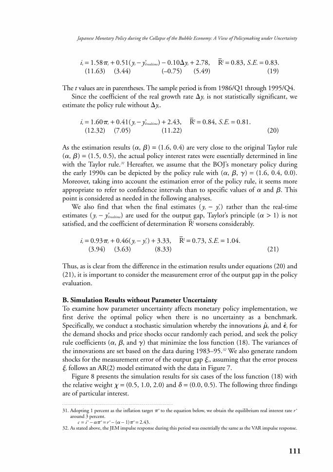
Figure 8 presents the simulation results for six cases of the loss function (18) with

the relative weight = (0.5, 1.0, 2.0) and � = (0.0, 0.5). The following three findings

are of particular interest.

111


31. Adopting 1 percent as the inflation target �* to the equation below, we obtain the equilibrium real interest rate r *

around 3 percent.c = i * − ��* = r * − (� − 1)�* = 2.43.

32. As stated above, the JEM impulse response during this period was essentially the same as the VAR impulse response.

First, when there is some weight on the interest rate smoothing � in the loss

function, it is desirable to set small values for all the policy rule coefficients (�, �, and

� ). This is because the stability of the inflation rate and of the output gap must be

sacrificed to smooth interest rate changes.

Second, as the relative weight on the output gap stabilization increases, it is

desirable to set higher values for the output gap coefficient � and the real growth rate

coefficient �, but a lower value for the inflation rate coefficient � of the policy rule.

This is because when the central bank faces a trade-off between the inflation rate

stabilization and the output gap stabilization, it cannot simultaneously achieve both.

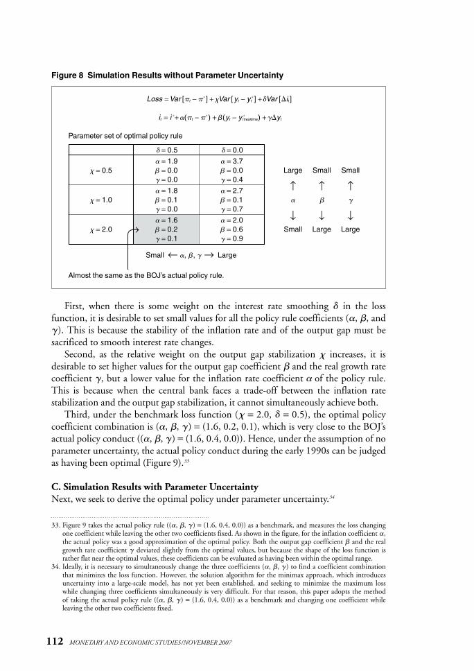
Third, under the benchmark loss function ( = 2.0, � = 0.5), the optimal policy

coefficient combination is (�, �, � ) = (1.6, 0.2, 0.1), which is very close to the BOJ’s

actual policy conduct ((�, �, � ) = (1.6, 0.4, 0.0)). Hence, under the assumption of no

parameter uncertainty, the actual policy conduct during the early 1990s can be judged

as having been optimal (Figure 9).33

C. Simulation Results with Parameter Uncertainty

Next, we seek to derive the optimal policy under parameter uncertainty.34


Figure 8 Simulation Results without Parameter Uncertainty

Loss = Var [�t − �*] + Var [yt − yt*] +�Var [�it ]

it = i *+ �(�t − �*) + �(yt − y *t |realtime) + ��yt

Parameter set of optimal policy rule

� = 0.5 � = 0.0

� = 1.9 � = 3.7 = 0.5 � = 0.0 � = 0.0 Large Small Small

� = 0.0 � = 0.4↑ ↑ ↑� = 1.8 � = 2.7

= 1.0 � = 0.1 � = 0.1 � � �� = 0.0 � = 0.7

↓ ↓ ↓� = 1.6 � = 2.0 = 2.0 � = 0.2 � = 0.6 Small Large Large

� = 0.1 � = 0.9

Small ← �, �, � → Large

Almost the same as the BOJ’s actual policy rule.

33. Figure 9 takes the actual policy rule ((�, �, � ) = (1.6, 0.4, 0.0)) as a benchmark, and measures the loss changingone coefficient while leaving the other two coefficients fixed. As shown in the figure, for the inflation coefficient �,the actual policy was a good approximation of the optimal policy. Both the output gap coefficient � and the realgrowth rate coefficient � deviated slightly from the optimal values, but because the shape of the loss function israther flat near the optimal values, these coefficients can be evaluated as having been within the optimal range.

34. Ideally, it is necessary to simultaneously change the three coefficients (�, �, � ) to find a coefficient combinationthat minimizes the loss function. However, the solution algorithm for the minimax approach, which introducesuncertainty into a large-scale model, has not yet been established, and seeking to minimize the maximum losswhile changing three coefficients simultaneously is very difficult. For that reason, this paper adopts the method of taking the actual policy rule ((�, �, � ) = (1.6, 0.4, 0.0)) as a benchmark and changing one coefficient whileleaving the other two coefficients fixed.

113


Figure 9 Policy Rule and Loss (� = 2.0, � = 0.5)

11

12

13

14

15

16

17

18

19

0.0 0.5 1.0 1.5Output gap coefficient:

11

12

13

14

15

16

17

18

19

–0.1 0.1 0.3 0.5 0.7 0.9 1.1 1.3 1.5Real growth rate coefficient:

11

12

13

14

15

16

17

18

19

1.0 1.5 2.0 2.5 3.0 3.5 4.0 4.5Inflation rate coefficient:

Loss

Loss

Loss

Actual policy rule

Minimum of loss

Actual policy rule

Actual policy rule

�

�

�

Minimum of loss

Minimum of loss

Loss = Var [�t − �*] + Var [yt − yt*] +�Var [�it ]

it = i *+ �(�t − �*) + �(yt − y *t |realtime) + ��yt

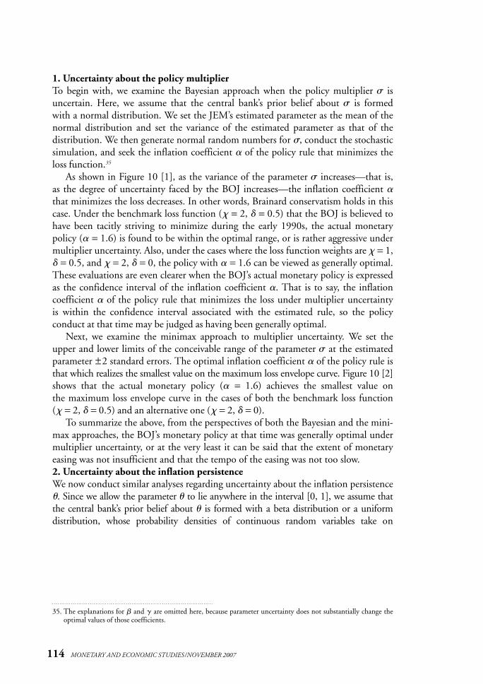
1. Uncertainty about the policy multiplier

To begin with, we examine the Bayesian approach when the policy multiplier � is

uncertain. Here, we assume that the central bank’s prior belief about � is formed

with a normal distribution. We set the JEM’s estimated parameter as the mean of the

normal distribution and set the variance of the estimated parameter as that of the

distribution. We then generate normal random numbers for �, conduct the stochastic

simulation, and seek the inflation coefficient � of the policy rule that minimizes the

loss function.35

As shown in Figure 10 [1], as the variance of the parameter � increases—that is,

as the degree of uncertainty faced by the BOJ increases—the inflation coefficient �that minimizes the loss decreases. In other words, Brainard conservatism holds in this

case. Under the benchmark loss function ( = 2, � = 0.5) that the BOJ is believed to

have been tacitly striving to minimize during the early 1990s, the actual monetary

policy (� = 1.6) is found to be within the optimal range, or is rather aggressive under

multiplier uncertainty. Also, under the cases where the loss function weights are = 1,

� = 0.5, and = 2, � = 0, the policy with � = 1.6 can be viewed as generally optimal.

These evaluations are even clearer when the BOJ’s actual monetary policy is expressed

as the confidence interval of the inflation coefficient �. That is to say, the inflation

coefficient � of the policy rule that minimizes the loss under multiplier uncertainty

is within the confidence interval associated with the estimated rule, so the policy

conduct at that time may be judged as having been generally optimal.

Next, we examine the minimax approach to multiplier uncertainty. We set the

upper and lower limits of the conceivable range of the parameter � at the estimated

parameter ±2 standard errors. The optimal inflation coefficient � of the policy rule is

that which realizes the smallest value on the maximum loss envelope curve. Figure 10 [2]

shows that the actual monetary policy (� = 1.6) achieves the smallest value on

the maximum loss envelope curve in the cases of both the benchmark loss function

( = 2, � = 0.5) and an alternative one ( = 2, � = 0).

To summarize the above, from the perspectives of both the Bayesian and the mini-

max approaches, the BOJ’s monetary policy at that time was generally optimal under

multiplier uncertainty, or at the very least it can be said that the extent of monetary

easing was not insufficient and that the tempo of the easing was not too slow.

2. Uncertainty about the inflation persistence

We now conduct similar analyses regarding uncertainty about the inflation persistence

�. Since we allow the parameter � to lie anywhere in the interval [0, 1], we assume that

the central bank’s prior belief about � is formed with a beta distribution or a uniform

distribution, whose probability densities of continuous random variables take on


35. The explanations for � and � are omitted here, because parameter uncertainty does not substantially change theoptimal values of those coefficients.

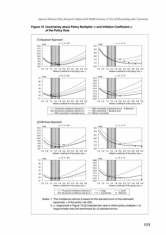
115


Figure 10 Uncertainty about Policy Multiplier � and Inflation Coefficient �of the Policy Rule

8.08.59.09.5

10.010.511.011.512.0

1.0 1.2 1.4 1.6 1.8 2.0 2.2 2.4 2.6 2.8 3.0

Loss Loss

6.5

7.0

7.5

8.0

8.5

9.0

9.5

11

12

13

14

15

16

17

10.010.511.011.512.012.513.013.514.0

8.08.59.09.5

10.010.511.011.512.0

6.5

7.0

7.5

8.0

8.5

9.0

9.5

11

12

13

14

15

16

17

10.010.511.011.512.012.513.013.514.0

Inflation coefficient of the policy rule: �1.0 1.2 1.4 1.6 1.8 2.0 2.2 2.4 2.6 2.8 3.0

Inflation coefficient of the policy rule: �

= 1, � = 0.5 = 1, � = 0

1.0 1.2 1.4 1.6 1.8 2.0 2.2 2.4 2.6 2.8 3.0

Loss Loss



= 2, � = 0.5 = 2, � = 0

1.0 1.2 1.4 1.6 1.8 2.0 2.2 2.4 2.6 2.8 3.0

Loss Loss

14.0



= 1, � = 0.5 = 1, � = 0

1.0 1.2 1.4 1.6 1.8 2.0 2.2 2.4 2.6 2.8 3.0

Loss Loss



= 2, � = 0.5 = 2, � = 0

70 percent confidence interval of90 percent confidence interval ofWith uncertainty, 3 standard errors

With uncertainty, 2 standard errorsWith uncertainty, 1 standard errorWithout uncertainty

Minimum��

70 percent confidence interval of90 percent confidence interval of

: large : benchmark

��

� : smallMinimum�

�

Notes: 1. The confidence interval is based on the standard error of the estimated parameter � of the policy rule (20).

2. �: large/small in Figure 10 [2] indicates the case in which policy multiplier � islarger/smaller than the benchmark by ±2 standard errors.

[1] Bayesian Approach

[2] Minimax Approach

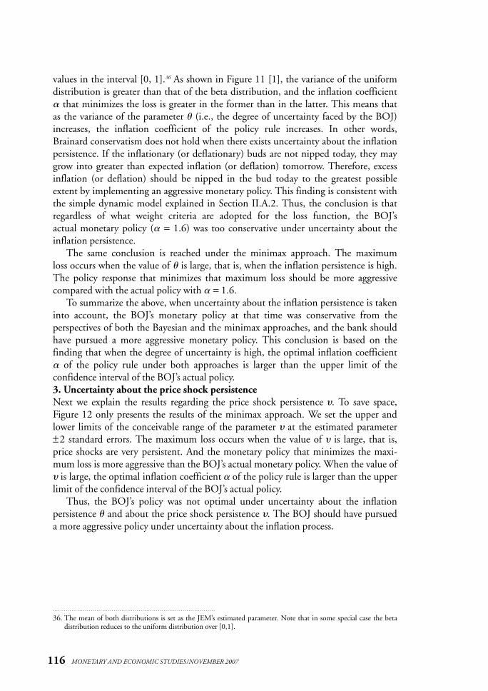
values in the interval [0, 1].36 As shown in Figure 11 [1], the variance of the uniform

distribution is greater than that of the beta distribution, and the inflation coefficient

� that minimizes the loss is greater in the former than in the latter. This means that

as the variance of the parameter � (i.e., the degree of uncertainty faced by the BOJ)

increases, the inflation coefficient of the policy rule increases. In other words,

Brainard conservatism does not hold when there exists uncertainty about the inflation

persistence. If the inflationary (or deflationary) buds are not nipped today, they may

grow into greater than expected inflation (or deflation) tomorrow. Therefore, excess

inflation (or deflation) should be nipped in the bud today to the greatest possible

extent by implementing an aggressive monetary policy. This finding is consistent with

the simple dynamic model explained in Section II.A.2. Thus, the conclusion is that

regardless of what weight criteria are adopted for the loss function, the BOJ’s

actual monetary policy (� = 1.6) was too conservative under uncertainty about the

inflation persistence.

The same conclusion is reached under the minimax approach. The maximum

loss occurs when the value of � is large, that is, when the inflation persistence is high.

The policy response that minimizes that maximum loss should be more aggressive

compared with the actual policy with � = 1.6.

To summarize the above, when uncertainty about the inflation persistence is taken

into account, the BOJ’s monetary policy at that time was conservative from the

perspectives of both the Bayesian and the minimax approaches, and the bank should

have pursued a more aggressive monetary policy. This conclusion is based on the

finding that when the degree of uncertainty is high, the optimal inflation coefficient

� of the policy rule under both approaches is larger than the upper limit of the

confidence interval of the BOJ’s actual policy.

3. Uncertainty about the price shock persistence

Next we explain the results regarding the price shock persistence �. To save space,

Figure 12 only presents the results of the minimax approach. We set the upper and

lower limits of the conceivable range of the parameter � at the estimated parameter

±2 standard errors. The maximum loss occurs when the value of � is large, that is,

price shocks are very persistent. And the monetary policy that minimizes the maxi-

mum loss is more aggressive than the BOJ’s actual monetary policy. When the value of

� is large, the optimal inflation coefficient � of the policy rule is larger than the upper

limit of the confidence interval of the BOJ’s actual policy.

Thus, the BOJ’s policy was not optimal under uncertainty about the inflation

persistence � and about the price shock persistence �. The BOJ should have pursued

a more aggressive policy under uncertainty about the inflation process.


36. The mean of both distributions is set as the JEM’s estimated parameter. Note that in some special case the beta distribution reduces to the uniform distribution over [0,1].

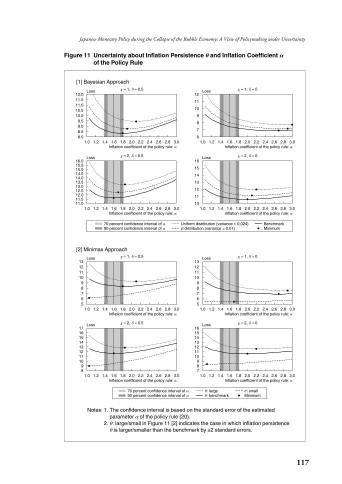
117


Figure 11 Uncertainty about Inflation Persistence � and Inflation Coefficient �of the Policy Rule

11.011.512.012.513.013.514.014.515.015.516.0

56789

10111213

56789

10111213

89

1011121314151617

789

10111213141516

10

11

12

13

14

15

16

6

7

8

9

10

11

12

8.08.59.09.5

10.010.511.011.512.0

1.0 1.2 1.4 1.6 1.8 2.0 2.2 2.4 2.6 2.8 3.0

Loss


= 1, � = 0.5

1.0 1.2 1.4 1.6 1.8 2.0 2.2 2.4 2.6 2.8 3.0Inflation coefficient of the policy rule: �

= 1, � = 0Loss

1.0 1.2 1.4 1.6 1.8 2.0 2.2 2.4 2.6 2.8 3.0

Loss Loss



= 2, � = 0.5 = 2, � = 0

1.0 1.2 1.4 1.6 1.8 2.0 2.2 2.4 2.6 2.8 3.0

Loss Loss



= 1, � = 0.5 = 1, � = 0

1.0 1.2 1.4 1.6 1.8 2.0 2.2 2.4 2.6 2.8 3.0

Loss Loss



= 2, � = 0.5 = 2, � = 0


: large : benchmark

��


�


Uniform distribution (variance = 0.024) distribution (variance = 0.01)

��

BenchmarkMinimum


2. �: large/small in Figure 11 [2] indicates the case in which inflation persistence� is larger/smaller than the benchmark by ±2 standard errors.

[1] Bayesian Approach

[2] Minimax Approach

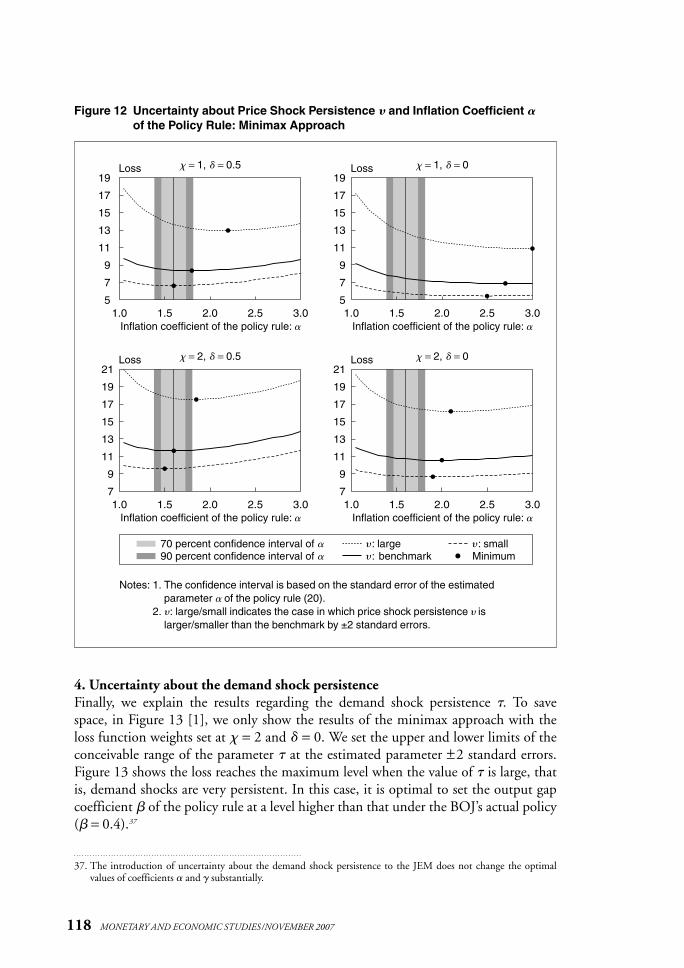
4. Uncertainty about the demand shock persistence

Finally, we explain the results regarding the demand shock persistence �. To save

space, in Figure 13 [1], we only show the results of the minimax approach with the

loss function weights set at = 2 and � = 0. We set the upper and lower limits of the

conceivable range of the parameter � at the estimated parameter ±2 standard errors.

Figure 13 shows the loss reaches the maximum level when the value of � is large, that

is, demand shocks are very persistent. In this case, it is optimal to set the output gap

coefficient � of the policy rule at a level higher than that under the BOJ’s actual policy

(� = 0.4).37


Figure 12 Uncertainty about Price Shock Persistence � and Inflation Coefficient �of the Policy Rule: Minimax Approach

5

7

9

11

13

15

17

19

1.0 1.5 2.0 2.5 3.05

7

9

11

13

15

17

19

7

9

11

13

15

17

19

21

7

9

11

13

15

17

19

21

Loss


= 1, � = 0.5

1.0 1.5 2.0 2.5 3.0

Loss


= 1, � = 0

1.0 1.5 2.0 2.5 3.0

Loss


= 2, � = 0.5

1.0 1.5 2.0 2.5 3.0

Loss


= 2, � = 0


: large : benchmark

��


�


2. � : large/small indicates the case in which price shock persistence � islarger/smaller than the benchmark by ±2 standard errors.

37. The introduction of uncertainty about the demand shock persistence to the JEM does not change the optimal values of coefficients � and � substantially.

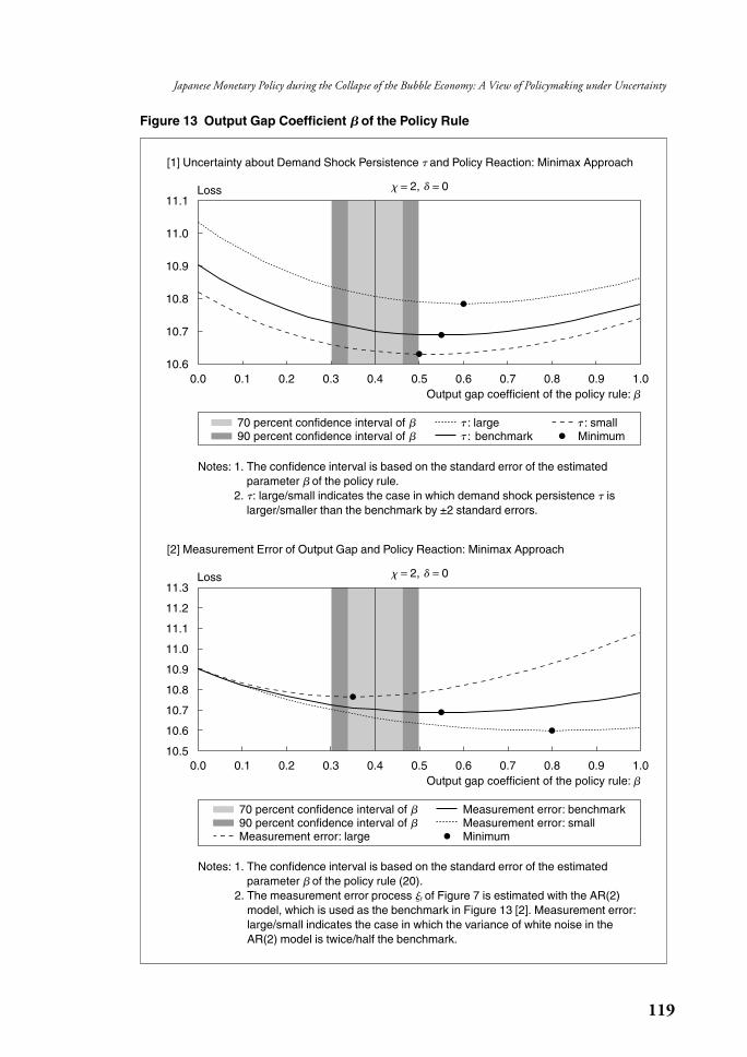
119


Figure 13 Output Gap Coefficient � of the Policy Rule

0.0 0.1 0.2 0.3 0.4 0.5 0.6 0.7 0.8 0.9 1.0Output gap coefficient of the policy rule: �

10.6

10.7

10.8

10.9

11.0

11.1Loss = 2, � = 0


: large : benchmark

��


�

[1] Uncertainty about Demand Shock Persistence � and Policy Reaction: Minimax Approach

10.6

10.7

10.8

10.9

11.0

11.1

11.2

11.3Loss

0.0 0.1 0.2 0.3 0.4 0.5 0.6 0.7 0.8 0.9 1.010.5

Output gap coefficient of the policy rule: �

= 2, � = 0

70 percent confidence interval of90 percent confidence interval ofMeasurement error: large

Measurement error: benchmarkMeasurement error: smallMinimum

��

[2] Measurement Error of Output Gap and Policy Reaction: Minimax Approach


2. The measurement error process �t of Figure 7 is estimated with the AR(2)model, which is used as the benchmark in Figure 13 [2]. Measurement error:large/small indicates the case in which the variance of white noise in theAR(2) model is twice/half the benchmark.

Notes: 1. The confidence interval is based on the standard error of the estimated parameter � of the policy rule.

2. �: large/small indicates the case in which demand shock persistence � islarger/smaller than the benchmark by ±2 standard errors.

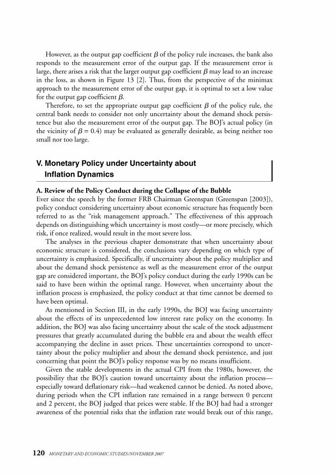
However, as the output gap coefficient � of the policy rule increases, the bank also

responds to the measurement error of the output gap. If the measurement error is

large, there arises a risk that the larger output gap coefficient � may lead to an increase

in the loss, as shown in Figure 13 [2]. Thus, from the perspective of the minimax

approach to the measurement error of the output gap, it is optimal to set a low value

for the output gap coefficient �.

Therefore, to set the appropriate output gap coefficient � of the policy rule, the

central bank needs to consider not only uncertainty about the demand shock persis-

tence but also the measurement error of the output gap. The BOJ’s actual policy (in

the vicinity of � = 0.4) may be evaluated as generally desirable, as being neither too

small nor too large.

V. Monetary Policy under Uncertainty about Inflation Dynamics

A. Review of the Policy Conduct during the Collapse of the Bubble

Ever since the speech by the former FRB Chairman Greenspan (Greenspan [2003]),

policy conduct considering uncertainty about economic structure has frequently been

referred to as the “risk management approach.” The effectiveness of this approach

depends on distinguishing which uncertainty is most costly—or more precisely, which

risk, if once realized, would result in the most severe loss.

The analyses in the previous chapter demonstrate that when uncertainty about

economic structure is considered, the conclusions vary depending on which type of

uncertainty is emphasized. Specifically, if uncertainty about the policy multiplier and

about the demand shock persistence as well as the measurement error of the output

gap are considered important, the BOJ’s policy conduct during the early 1990s can be

said to have been within the optimal range. However, when uncertainty about the

inflation process is emphasized, the policy conduct at that time cannot be deemed to

have been optimal.

As mentioned in Section III, in the early 1990s, the BOJ was facing uncertainty

about the effects of its unprecedented low interest rate policy on the economy. In

addition, the BOJ was also facing uncertainty about the scale of the stock adjustment

pressures that greatly accumulated during the bubble era and about the wealth effect

accompanying the decline in asset prices. These uncertainties correspond to uncer-

tainty about the policy multiplier and about the demand shock persistence, and just

concerning that point the BOJ’s policy response was by no means insufficient.

Given the stable developments in the actual CPI from the 1980s, however, the

possibility that the BOJ’s caution toward uncertainty about the inflation process—

especially toward deflationary risk—had weakened cannot be denied. As noted above,

during periods when the CPI inflation rate remained in a range between 0 percent

and 2 percent, the BOJ judged that prices were stable. If the BOJ had had a stronger

awareness of the potential risks that the inflation rate would break out of this range,


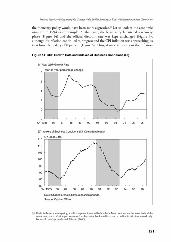
the monetary policy would have been more aggressive.38 Let us look at the economic

situation in 1994 as an example. At that time, the business cycle entered a recovery

phase (Figure 14) and the official discount rate was kept unchanged (Figure 3),

although disinflation continued to progress and the CPI inflation was approaching its

tacit lower boundary of 0 percent (Figure 6). Thus, if uncertainty about the inflation

121


Figure 14 GDP Growth Rate and Indexes of Business Conditions (CI)

–2

0

2

4

6

8

1985 86 87 88 89 90 91 92 93 94 95 96


CY

[1] Real GDP Growth Rate

1985 86 87 88 89 90 91 92 93 94 95 96CY80

85

90

95

100

105

110

115CY 2000 = 100

[2] Indexes of Business Conditions (CI, Coincident Index)

Note: Shaded areas indicate recession periods.

Source: Cabinet Office.

38. Under inflation zone targeting, a policy response is needed before the inflation rate reaches the lower limit of thetarget zone, since inflation persistence makes the central bank unable to stop a decline in inflation immediately.For details, see Orphanides and Wieland (2000).

process such as the continued appreciation of the yen was emphasized, criticism that

the central bank should have implemented monetary easing within 1994 may be

warranted. However, what was recognized at that time was primarily the downside risk

from the influence of the yen’s appreciation on the real economy, and there was almost

no discussion regarding the deflationary concerns for general prices.39 This indicates

that when adopting the risk management approach, it is important to distinguish

which uncertainty confronting the central bank is most costly—or more precisely,

which risk, if once realized, would result in the most severe loss.

B. Relative Weight on the Price Stability and Uncertainty about

the Inflation Persistence

The analyses in Section IV are based on given weights (, �) for the loss function

(18). However, New Keynesian economics suggests that as the degree of uncertainty

about inflation dynamics increases the central bank should place much more weight on

the price stability, that is, reduce the values of and �.40 This subsection summarizes the

background to this way of thinking.

The absolute value of social welfare losses is expressed by the following equation.

�Var [�t − �*] + yVar [yt − y*t ] + iVar [�it ]. (22)

The loss function (18) and the relative weight have the following relationship.

= y /�, � = i /�. (23)

The first term of equation (22), �Var [�t − �*], is the welfare cost of inflation

volatility, and the parameter � has a close relationship with the parameter �, which

measures the inflation persistence.41 In the Phillips curve (10), it is assumed that a

fraction 1 – � of firms set prices based on marginal costs in a forward-looking manner

and the remaining fraction � uses a backward-looking rule to set prices (0 ≤ � ≤ 1).

An increase in the fraction � has highly persistent effects on the relative price disper-

sion across firms, and hence fluctuations in aggregate inflation increase welfare cost.

This means that as the fraction � increases, the parameter � rises. Simultaneously,

an increase in the fraction � makes inflation more persistent, that is, it raises the

parameter � of the Phillips curve. In other words, the root of the inflation persistence

lies in the existence of firms that use a backward-looking rule to set prices, and the

uncertainty about the inflation persistence results from the central bank’s lack of

information regarding the fraction � of firms that use a backward-looking rule. When

the fraction � is uncertain for the central bank, it faces both uncertainty about the

inflation persistence � and about the welfare parameter �.


39. Jinushi, Kuroki, and Miyao (2000) criticize the BOJ for leaving the official discount rate unchanged in 1994: “A further loosening in 1994 might have prevented the abnormal yen appreciation in March 1995 and might have accomplished stronger recovery afterward.” However, this is only a retrospective argument from the hindsightof 2001.

40. See Kimura and Kurozumi (2007) and Walsh (2005).41. For details, see Kimura, Fujiwara, and Kurozumi (2005).

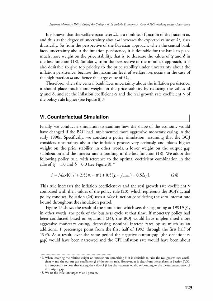
It is known that the welfare parameter � is a nonlinear function of the fraction �,

and thus as the degree of uncertainty about � increases the expected value of � rises

drastically. So from the perspective of the Bayesian approach, when the central bank

faces uncertainty about the inflation persistence, it is desirable for the bank to place

much more weight on the price stability, that is, to decrease the values of and � in

the loss function (18). Similarly, from the perspective of the minimax approach, it is

also desirable to give top priority to the price stability under uncertainty about the

inflation persistence, because the maximum level of welfare loss occurs in the case of

the high fraction � and hence the large value of �.

Therefore, when the central bank faces uncertainty about the inflation persistence,

it should place much more weight on the price stability by reducing the values of

and �, and set the inflation coefficient � and the real growth rate coefficient � of

the policy rule higher (see Figure 8).42

VI. Counterfactual Simulation

Finally, we conduct a simulation to examine how the shape of the economy would

have changed if the BOJ had implemented more aggressive monetary easing in the

early 1990s. Specifically, we conduct a policy simulation, assuming that the BOJ

considers uncertainty about the inflation process very seriously and places higher

weight on the price stability, in other words, a lower weight on the output gap

stabilization and the interest rate smoothing in the loss function (18). We adopt the

following policy rule, with reference to the optimal coefficient combination in the

case of = 1.0 and � = 0.0 (see Figure 8).43

it = Max [0, i * + 2.5(�t − �*) + 0.5(yt − y*t|realtime) + 0.5�yt]. (24)

This rule increases the inflation coefficient � and the real growth rate coefficient �compared with their values of the policy rule (20), which represents the BOJ’s actual

policy conduct. Equation (24) uses a Max function considering the zero interest rate

bound throughout the simulation period.

Figure 15 shows the result of the simulation which sets the beginning at 1991/Q1,

in other words, the peak of the business cycle at that time. If monetary policy had

been conducted based on equation (24), the BOJ would have implemented more

aggressive monetary easing, decreasing nominal interest rates by as much as an

additional 1 percentage point from the first half of 1993 through the first half of

1995. As a result, over the same period the negative output gap (the deflationary

gap) would have been narrowed and the CPI inflation rate would have been about

123


42. When lowering the relative weight on interest rate smoothing �, it is desirable to raise the real growth rate coeffi-cient � and the output gap coefficient � of the policy rule. However, as is clear from the analyses in Section IV.C, it is important to note that raising the value of � has the weakness of also responding to the measurement error ofthe output gap.

43. We set the inflation target �* at 1 percent.

0.2 percentage point higher than its actual levels. Subsequently, in the late 1990s the

CPI inflation would have continued to be higher than actual.

However, as shown in Figure 15, aggressive monetary policy would not have

resulted in an outstanding reduction in the deflationary gap.44 This is because the

stock adjustment pressures and balance-sheet adjustment pressures from the collapse

of the bubble were strong. Similarly, there was a great influence of the credit crunch

that resulted from the financial system shock at the end of 1997, so the deflationary

gap would have remained substantial through 1998. As a result, even under an

aggressive policy response the CPI inflation would have been driven back into

negative territory once again in 2000.

The above simulation indicates that while a more aggressive policy response

following the collapse of the bubble would have provided some underpinning to the


Figure 15 Counterfactual Simulation

–3

–2

–1

0

1

2

3

–3–2–10123456789

1991FY 92 93 94 95 96 97 98 99 2000 01

Percent

1991FY 92 93 94 95 96 97 98 99 2000 01

Percent

[1] Nominal Short-Term Interest Rate(3 Months)

[2] Output Gap

–2

–1

0

1

2

3

1991FY 92 93 94 95 96 97 98 99 2000 01


1991FY 92 93 94 95 96 97 98 99 2000 01


–3

–2

–1

0

1

2

3

4

5

6

ActualDifference between simulation and actual

Simulation of aggressive monetary policy

[3] CPI (Excluding Perishables andPublic Utilities Charge)

[4] GDP Growth Rate

Sources: Bank of Japan; Cabinet Office; Ministry of Internal Affairs and Communications.

44. In the JEM, these two adjustment pressures are represented by the negative demand shock t < 0 in the IS curve (11).

inflation rate and the real growth rate, its effect would have been limited and just

implementing monetary easing earlier would not have changed the overall image of

the prolonged stagnation of the 1990s.45

VII. Conclusions

To date, diverse debates have developed regarding the prolonged stagnation of the

Japanese economy during the 1990s. Broadly speaking, there are two main ways of

thinking regarding the prolonged stagnation: the supply-side view (decline in the

potential growth rate); and the demand-side view (insufficient demand). As a specific

example of the demand-side view, we examined the position asserted by many advocates

that “the delay in monetary easing in the early 1990s caused insufficient demand.”

We found that the BOJ’s policy at that time was basically optimal under uncertainty

about the policy multiplier, but that the policy was not optimal under uncertainty

about the inflation process and a more aggressive policy response would have been

needed. Considering the fact that the Japanese economy fell into a deflationary

state from the late 1990s, it seems difficult to deny that in the early 1990s the BOJ

should have placed greater emphasis on uncertainty about the inflation process and

implemented monetary easing earlier. Nevertheless, the counterfactual simulation

indicates that more aggressive monetary easing would not have changed the overall

image of the prolonged stagnation. In this sense, the position that the delay in

monetary easing was the primary cause of the prolonged stagnation is not supported.

A more appropriate viewpoint is that in addition to both demand and supply side

problems, the prolonged stagnation resulted from multiple factors such as the

nonperforming-loan problem and other deterioration in bank functions.

In closing, as an implication derived from our analyses, we would like to note

that the policy judgment of where the greatest risk lies is a critical point in risk

management. Our analyses do indicate that in the early 1990s the BOJ should have

given greater emphasis to uncertainty about the inflation process over multiplier

uncertainty, but this does not imply that the former will constitute the greater risk

at all times in the future. It is necessary to examine in real time what is the greatest

risk in the economic assessment.

125


45. Kawasaki and Aoki (2004) conduct a simulation using a macroeconometric model of the Japanese economy andderive results similar to ours. On the other hand, Ahearne et al. (2002) derive the conclusion that deflation couldhave been avoided if interest rates had been permanently decreased by 2.5 percentage points from their actual levels in the early 1990s. However, a 2.5 percentage point decrease in the interest rate can be considered an unrealistic setting that cannot be derived under any optimal rule in Figure 8.

Ahearne, Alan G., Joseph E. Gagnon, Jane Haltmaier, Steven B. Kamin, Christopher J. Erceg, Jon Faust,

Luca Guerrieri, Carter Hemphill, Linda Kole, Jennifer E. Roush, John H. Rogers, Nathan Sheets,

and Jonathan H. Wright, “Preventing Deflation: Lessons from Japan’s Experience in the 1990s,”

International Finance Discussion Paper No. 729, Board of Governors of the Federal Reserve

System, 2002.

Angeloni, Ignazio, Günter Coenen, and Frank Smets, “Persistence, the Transmission Mechanism and

Robust Monetary Policy,” ECB Working Paper No. 250, European Central Bank, 2003.

Bernanke, Ben, and Mark Gertler, “Monetary Policy and Asset Price Volatility,”Economic Review, Federal

Reserve Bank of Kansas City, Fourth Quarter, 1999, pp. 17–51.

Blinder, Alan, Central Banking in Theory and Practice, Cambridge, Massachusetts: The MIT Press, 1998.

Brainard, William, “Uncertainty and the Effectiveness of Policy,” American Economic Review, 57 (2),

1967, pp. 411–425.

Calvo, Guillermo A., “Staggered Prices in a Utility-Maximizing Framework,” Journal of Monetary

Economics, 12 (3), 1983, pp. 383–398.

Erceg, Christopher J., and Andrew T. Levin, “Optimal Monetary Policy with Durable and Non-Durable

Goods,” ECB Working Paper No. 179, European Central Bank, 2002.

Fujiwara, Ippei, Naoko Hara, Yasuo Hirose, and Yuki Teranishi, “The Japanese Economic Model

(JEM),” Monetary and Economic Studies, 23 (2), Institute for Monetary and Economic Studies,

Bank of Japan, 2005, pp. 61–142.

Giannoni, Marc, “Optimal Interest-Rate Rules in a Forward-Looking Model, and Inflation Stabilization

versus Price-Level Stabilization,” mimeo, Federal Reserve Bank of New York, 2000.

———, “Does Model Uncertainty Justify Caution? Robust Optimal Monetary Policy in a Forward-

Looking Model,” Macroeconomic Dynamics, 6 (1), 2002, pp. 111–144.

———, “Robust Optimal Monetary Policy in a Forward-Looking Model with Parameter and Shock

Uncertainty,” NBER Working Paper No. 11942, National Bureau of Economic Research, 2006

(also forthcoming in the Journal of Applied Econometrics ).

Goodfriend, Marvin, “Interest Rates and the Conduct of Monetary Policy,”Carnegie-Rochester Conference

Series on Public Policy, 34, 1991, pp. 7–30.

Goodhart, Charles, “Central Bankers and Uncertainty,” Bank of England Quarterly Bulletin, Bank of

England, February, 1999, pp. 102–121.

Greenspan, Alan, “Monetary Policy and Uncertainty: Adapting to a Changing Economy,” remarks at a

symposium sponsored by the Federal Reserve Bank of Kansas City, Jackson Hole, Wyoming,

August 28, 2003.

Hamada, Koichi, “Keizai-Gaku no Murikai ga Shinka Saseta Heisei-Fukyo (Japanese Stagnation in 1990s

Caused by Misunderstanding of Economics),” in Koichi Hamada and Akiyoshi Horiuchi, eds.

Ronso Nihon no Keizai Kiki—Choki Teitai no Shinin wo Kaimeisuru (Japan’s Economic Crisis),

Nihon Keizai Shimbunsha, 2004, pp. 318–336 (in Japanese).

Hansen, Lars P., and Thomas J. Sargent, “Robust Control of Forward-Looking Models,” Journal of

Monetary Economics, 50 (3), 2003, pp. 581–604.

Jinushi, Toshiki, Yoshihiro Kuroki, and Ryuzo Miyao, “Monetary Policy in Japan since the Late 1980s:

Delayed Policy Actions and Some Explanations,” in Ryoichi Mikitani and Adam S. Posen, eds.

Japan’s Financial Crisis and Its Parallels to U.S. Experience, Institute for International Economics,

2000, pp. 115–148.

Kawasaki, Kenichi, and Daiju Aoki, “Macro Keiryo Model ni Yoru Rekishiteki Simulation: 1990-Nendai

no Kin’yu Seisaku no Koka (Historical Simulation Using a Macroeconometric Model: Effect of

Monetary Policy in 1990s),” in Koichi Hamada and Yutaka Harada, eds. Choki Fukyo no Riron

to Jissho (Theories and Empirical Analyses of the Prolonged Stagnation), Toyo Keizai Shimposha,

2004, pp. 147–164 (in Japanese).

Kimura, Takeshi, Ippei Fujiwara, and Takushi Kurozumi, “Shakai no Keizai Kosei to Kin’yu Seisaku no

Mokuteki (Social Welfare and the Goal of Monetary Policy),” Bank of Japan Review Paper No.

2005-J-9, Bank of Japan, 2005 (in Japanese).


References

———, and Takushi Kurozumi, “Effectiveness of History-Dependent Monetary Policy,” Journal of the

Japanese and International Economies, 18 (3), 2004, pp. 330–361.

———, and ———, “Optimal Monetary Policy in a Micro-Founded Model with Parameter

Uncertainty,” Journal of Economic Dynamics and Control, 31 (2), 2007, pp. 399–431.

McCallum, Bennett T., “Japanese Monetary Policy,” mimeo, 2001.

Meese, Richard A., and Kenneth Rogoff, “Empirical Exchange Rate Models of the Seventies: Do They

Fit Out of Sample?” Journal of International Economics, 14, 1983, pp. 3–24.

Mori, Naruki, Shigenori Shiratsuka, and Hiroo Taguchi, “Policy Responses to the Post-Bubble

Adjustments in Japan: A Tentative Review,” Monetary and Economic Studies, 19 (S-1), Institute

for Monetary and Economic Studies, Bank of Japan, 2001, pp. 53–102.

Noguchi, Asahi, and Yasushi Okada, “Kin’yu Seisaku no Kinoteishi ha Naze Shojitanoka (Why Did

Monetary Policy Fail?),” in Kikuo Iwata and Tsutomu Miyagawa, eds. Ushinawareta 10-Nen no

Shinin ha Nanika (What Caused Japan’s Prolonged Stagnation in 1990s?), Toyo Keizai

Shimposha, 2003, pp. 79–105 (in Japanese).

Okada, Yasushi, and Yasuyuki Iida, “Kin’yu Seisaku no Shippai ga Maneita Choki Teitai (Prolonged

Stagnation Caused by Monetary Policy Failure),” in Koichi Hamada and Akiyoshi Horiuchi, eds.

Ronso Nihon no Keizai Kiki—Choki Teitai no Shinin wo Kaimeisuru (Japan’s Economic Crisis),

Nihon Keizai Shimbunsha, 2004, pp. 149–174 (in Japanese).

Okina, Kunio, and Shigenori Shiratsuka, “Asset Price Bubbles, Price Stability, and Monetary Policy: Japan’s

Experience,” Monetary and Economic Studies, 20 (3), Institute for Monetary and Economic

Studies, Bank of Japan, 2002, pp. 35–76.

Onatski, Alexei, and James H. Stock, “Robust Monetary Policy under Model Uncertainty in a Small

Model of the U.S. Economy,” Macroeconomic Dynamics, 6 (1), 2002, pp. 85–110.

Orphanides, Athanasios, “Monetary Policy Rules Based on Real-Time Data,”American Economic Review,

91 (4), 2001, pp. 964–985.

———, “The Quest for Prosperity without Inflation,” Journal of Monetary Economics, 50 (3), 2003,

pp. 633–663.

———, Richard D. Porter, David Reifschneider, Robert Tetlow, and Frederico Finan, “Errors in the

Measurement of the Output Gap and the Design of Monetary Policy,” Finance and Economics

Discussion Paper No. 45, Board of Governors of the Federal Reserve System, 1999.

———, and Volker Wieland, “Inflation Zone Targeting,” European Economic Review, 44 (7), 2000,

pp. 1351–1387.

Roberts, John M., “New Keynesian Economics and the Phillips Curve,” Journal of Money, Credit and

Banking, 27 (4), 1995, pp. 975–984.

Rotemberg, Julio J., and Michael Woodford, “An Optimization-Based Econometric Framework for

the Evaluation of Monetary Policy,” in Ben S. Bernanke and Julio J. Rotemberg, eds. NBER

Macroeconomics Annual 1997, Cambridge, Massachusetts: The MIT Press, 1997, pp. 297–346.

Rudebusch, Glenn D., “Is the Fed Too Timid? Monetary Policy in an Uncertain World,” Review of

Economics and Statistics, 83 (2), 2001, pp. 203–217.

———, “Assessing the Lucas Critique in Monetary Policy Models,” Journal of Money, Credit and

Banking, 37 (2), 2005, pp. 245–272.

Saita, Yumi, Izumi Takagawa, Kenji Nishizaki, and Masahiro Higo, “Kori Bukka Tokei Chosa wo

Mochiita Kakaku Nenchakusei no Keisoku (Price Setting in Japan: Evidence from CPI Micro

Data),” BOJ Working Paper No. J-17, Bank of Japan, 2006 (in Japanese).

Sargent, Thomas J., “Comment,” in John B. Taylor, ed. Monetary Policy Rules, Chicago: University of

Chicago Press, 1999, pp. 144–154.

Söderström, Ulf, “Monetary Policy with Uncertain Parameters,” Scandinavian Journal of Economics, 104,

2002, pp. 125–145.

Stock, James H., “Comment,” in John B. Taylor, ed. Monetary Policy Rules, Chicago: University of

Chicago Press, 1999, pp. 253–259.

Tanaka, Hidetaka, and Takeshi Kimura, “Vector Error Correction Model wo Mochiita Bukka no Kettei

Mechanism ni Kansuru Jissho Bunseki (Empirical Analysis of Price Determination Mechanism

Using Vector Error Correction Model),” Research and Statistics Department Working Paper

No. 10, Bank of Japan, 1998 (in Japanese).

127


Taylor, John B., “Aggregate Dynamics and Staggered Contracts,” Journal of Political Economy, 88, 1980,

pp. 1–23.

———, “Discretion versus Policy Rules in Practice,” Carnegie-Rochester Conference Series on Public

Policy, 39, 1993, pp. 195–214.

———, “Low Inflation, Deflation, and Policies for Future Price Stability,” Monetary and Economic

Studies, 19 (S-1), Institute for Monetary and Economic Studies, Bank of Japan, 2001, pp. 35–51.

Walsh, Carl E., “Endogenous Objectives and the Evaluation of Targeting Rules for Monetary Policy,”

Journal of Monetary Economics, 2005, 52 (5), pp. 889–911.

Watanabe, Tsutomu, “Output Gap and Inflation: the Case of Japan,” Monetary Policy and the Inflation

Process, BIS Conference Paper No. 4, Bank for International Settlements, 1997.

Williams, John C., “Robust Estimation and Monetary Policy with Unobserved Structural Change,”

Working Paper in Applied Economic Theory No. 11, Federal Reserve Bank of San Francisco,

2004.


Japanese Monetary Policy during the Collapse of the Bubble ...

Documents

Transcript of Japanese Monetary Policy during the Collapse of the Bubble ...