1

January 2014 APEC RR14-02

Working paper on

Valuing Continuously Varying Visual

Disamenities: Offshore Energy Production

and Delaware Beach Visitation

Jacob Fooks

Kent Messer

Josh Duke

Janet Johnson

George Parsons

F

RE

C R

esearch R

epo

rts D

ep

artm

en

t of F

oo

d a

nd

Res

ou

rce

Ec

on

om

ics

• Co

lleg

e o

f Ag

ricu

lture

an

d N

atu

ral R

es

ou

rce

s • U

niv

ers

ity o

f Dela

wa

re

A

PE

C R

esearch R

epo

rts D

ep

artm

en

t of A

pp

lied

Ec

on

om

ics

ad

Sta

tistic

s • C

olle

ge

of A

gric

ultu

re a

nd

Na

tura

l Res

ou

rce

s • U

niv

ers

ity o

f Dela

wa

re

APPLIED

ECONOMICS

& STATISTICS

2

Abstract

This research proposes a new approach to measuring and estimating Willingness to Pay (WTP) for a

variety of non-market amenities. The continuous variation of attributes present in many non-market

goods is utilized to collect higher resolution information on consumers' choices concerning their use

decisions than is available through standard dichotomous choice questions. It does this without directly

asking research participants to form explicit valuations - an unfamiliar and cognitively challenging task

for most consumers. This generates data that can be estimated with a duration, or survival model

consistent with Random Utility Theory, from which an expression for WTP as a function of the

continuous attribute can be recovered. We apply this approach to estimate Delaware beach visitors'

visual disamenity from the presence of offshore energy generation installations.

3

Valuing Continuously Varying Visual Disamenities: Offshore Energy Production and

Delaware Beach Visitation

Jacob Fooks, Kent Messer, Josh Duke, Janet Johnson, and George Parsons

Introduction

Dichotomous choice questions have been the de facto elicitation format for

environmental valuation studies since the Arrow et al. (1995) NOAA report on Contingent

Valuation endorsed it as the standard for such work. One of the primary rationales for this

standard is that the dichotomous choice format poses questions in the attribute acceptance

domain given a posted price. This contrasts with direct response formats such as open ended or

payment ladder elicitation questions which seek a response in terms of Willingness-to-Pay

(WTP) given a set of attributes. The upside of questions that directly measure WTP is very

precise observations, generally either a point or small interval. Dichotomous choice responses

only offer yes/no responses at a few fixed prices so tend to require a much larger sample to

obtain the same level of accuracy (Cameron and Quiggin, 1994). However, as consumers,

research participants typically are much more familiar with posted price decision making. They

are comfortable assessing whether they would be willing to accept an offered deal. The question

of exactly how much they would be willing to pay for some hypothetical package of attributes is

much more cognitively taxing and therefore, it is contended, more prone to bias. Exactly how

substantial this bias is has been debated, and likely depends on the familiarity of the situation and

the design of the elicitation instrument (Balistreri et al., 2001).

There have been attempts to improve the efficiency of dichotomous choice instruments.

A notable example is the double bound, or interval method which asks a yes/no WTP question at

a certain price level, and then depending on the response, asks a follow-up at a second price level

either above or below the initial price level (Albeini, 1995). This keeps the decision in the

4

posted price decision space, but considerably improves the statistical efficiency of collected data

(Hanemann, Loomis, and Kanninen ,1991). However Cameron et al. (1996) observe a level of

inconsistency between initial and follow-up WTP distributions, and speculate that by introducing

a new price-point may cause participants to update their WTP distribution. This would be

consistent with theories of value formation (Plott, 1996).

We propose a "follow-up-question" approach that takes advantage of the fact that the

non-market goods' attributes of interest frequently have a continuously varying component.

Often this may be an explicitly spatial component, such as distance to public spaces (Borchers

and Duke, 2012), from hydraulic fracturing wells (Popkin, et al., forthcoming), or width of

restored beaches (Parsons, et al., 2013). Alternately, it could be something less distance-like,

such as the level of contamination of drinking water (Messer, 2009). In these cases, surveys can

be designed in a "simulation" format. Using technology and drawing on approaches from

experiential surveying and experiment techniques, we have participants respond in terms of level

of attribute given a set price. This can be repeated at different price levels and with different

attributes to obtain a series of observed intervals of attribute acceptance that can be modeled with

standard duration, or survival models that typically estimate effects on the time to some event. It

has been observed that when time is replaced with cost, duration models become estimates of

demand curves (Steinberg and Carson, 1989). Use of duration models to estimate WTP is

common in both payment ladder valuation data (Wang and He, 2011) and medical treatment data

(Luchini, Daoud, and Moatti, 2007). In the methods section we show that when specified in term

of attribute level with cost as a covariate, it is possible to recover an estimate of WTP as a

function of the attribute level at the mean, median, or for a specific consumer.

5

Duration models are standard in many econometric packages and offer a great deal of

"out of the box" flexibility when dealing with issues like censoring and unobserved

heterogeneity. They are also consistent with the Random Utility Model that motivates the

empirical models used to analyze dichotomous choice data, with the added benefit of greater

statistical power given data collection constraints. We use a Monte Carlo experiment to compare

the WTP recovered from a duration model with that from a multiple dichotomous choice design

estimated using a logit model. We find a significant difference between the two for moderate

sample sized. With samples of around 60 - 80 respondents the standard errors produced by the

duration model are on the order of half of those of the dichotomous choice data.

Following the presentation of this duration based method, a demonstration is offered

using data collected from Delaware beach visitors to estimate the value of the visual disamenity

generated by offshore energy production. We intercepted visitors on the beach, gathered their

trip cost data, and had them participate in a computer simulation showing them a picture of the

beach that they were standing on with wind turbines and oil platforms overlaid on the horizon.

They had the opportunity to adjust the location of the turbines or platforms to the point at which

they would no longer be willing to visit the beach at several randomly assigned price discounts.

This data was used to estimate a model of visitor attrition with distance of energy generation

infrastructure, with co-varying trip costs, energy type, and demographics. We find that visitors

are fairly indifferent of wind turbines up to 2-3 miles offshore, are less accepting of oil

platforms, and have a lower price elasticity of demand for platforms relative to turbines.

Methods

6

. Like double-bound designs, we start with a dichotomous (accept or reject) choice for a

fixed attribute bundle. Once they have made their choice they may adjust the bundle to decrease

to the point at which that answer would no longer be true; in essence reducing their surplus to

zero?? their approximate reservation utility. The key here is that instead of adjusting price,

research participants are given a fixed price and asked to adjust the continuously varying

attribute to achieve a fixed (reservation) level of utility. They are then offered a new fixed price

through a plausible payment mechanism, and adjust the attribute to a new level, consistent with

reservation utility at that new price. By observing several price/attribute pairs at the reservation

utility level, we are able to trace out the shape of an indifference curve through the reservation

utility and locate it in price/attribute space, as described below.

We developed a survey instrument that allows participants to adjust the attribute of

interest giving participants a realistic depiction of the results of their choices. In the project

described more fully below, participants on the beach, viewed a computer simulation showing an

image of that beach with realistic wind turbines and oil platforms on the horizon that they could

scroll in and out. This gave them a decision environment that is much more concrete than an

abstract decision in terms of hypothetical monetary values.

Estimation Approach

Consider an individual i’s choice of an outcome from a set of several possible options.

According to the Random Utility Model, they will choose a particular outcome of interest, j=1, if

they believe that the utility associated with outcome j = 1 exceeds the utility of all other

outcomes; in particular the outcome of their next best option, j = -1:

7

The indirect utility functions for both utilities will be a function of the price associated with that

outcome, pi,j, and a vector of other individual and outcome specific attributes, zi,j. Suppose that

outcome j=1 has an attribute of interest that may take values over some set range,

that has some effect on the utility of the outcome, but not on the other alternative1. If we assume

that the utility of the beach visit is linear in wd, we can write:

( )

( )

Conditional on price and attributes, the probability of an individual choosing option j=1 can be

expressed as:

[ ( ) | ] [ ( ) ( ) | ]

[

[ ( ) ( ) ]| ]

|

( )

We can think of Ui,-1 as being a reservation utility with the distribution of Ui,-1|pi,zi

inherited from εi,-1. U* is a random variable representing a scaled premium in utility for j=1 when

is at the furthest bound of its range, . This will be a random variable with cumulative

distribution ( ) ∫ ( )

. The function S(wd) is very similar to a survival function as is

commonly used in duration analysis, except that in this case it is a function of wd instead of time.

If an instrument can be developed that can solicit participant decisions in terms of a “withdrawal

1 Note that in this case we assume that decreasing values of attribute w have a negative effect on utility. The

opposite could be easily accommodated by switching signs in the derivation of WTP from the hazard functions specified below.

8

point2,” we can estimate the Random Utility Model using a duration approach using standard

econometric software and interpret the results using similar techniques. It will also be useful to

consider the hazard function, ( ) ( ) ( ) ⁄ The survival function, S(wd), indicates

the probability that an individual will continue to choose outcome j=1 for w<wd, while λ(wd)

indicates an instantaneous likelihood of switching to the next best option at wd.

The distribution of U*|pi,zi , and hence the parametric specification of the duration model

will depend on the distributions of εi,1 and εi,-1. Under the common assumption that these are both

Extreme Value Type I (EV.I) distributions, U*|pi,zi will be logistic, and the estimated duration

model will be log-logistic. If we assume that both are Normal distributions, U*|pi,zi will be

normal, and the estimated duration model will be log-normal. If we assume that the disturbance

on the outcome j=1 utility is EV.I, while the reservation utility is normal, then the difference will

be an EV distribution, and the duration model can be specified as a Weibull model3. In practice,

the choice between these models is often guided by the data, either through parameter

significance tests for nested distributions (several of the distributions used in duration analysis

are of the exponential family and are nested through restrictions on estimated parameters) , or

more generally through comparison of Akaike information criterion (AIC).

From an estimated duration model, a hazard model generally can be easily recovered.

When the results are specified in hazard form a willingness to pay is calculated from the

estimation results. With payment included as a covariate in the model, the fully augmented

hazard function will be λ(wd; pi,zi). Then, the required compensation to maintain the same

probability of switching to the alternative, and hence the same level of utility, will solve

3 A Weibull specification is one of the more commonly used in duration analysis, and has the advantage of a

relatively clean hazard function, and a resulting WTP function that depends only on p and w.

9

( ) ( ( ) ). A solution for C as a function of wd will depend on

distributional assumptions. Notably, if we consider X to be the full covariate vector, β to be the

vector of regression coefficients, βp to be the price coefficient, and γ and ρ to be shape

parameters of Weibull and log-logistic distributions respectively, then

- If the model is Weibull, the hazard ratio is of the form:

( )

and WTP will satisfy:

( ) [

] [

]

- If the model is log-logistic, the hazard ratio is of the form:

( ) ( ⁄ )

(

⁄ )

( )

and WTP will satisfy:

( )

{[

]

( )

[

] [

] [ ]}

Note that C in the case of the Weibull distribution is a function only of the price parameter, and

will be constant across the population, while for the log-logistic distribution it is a function of the

full parameter vector and individual attributes so it will vary across individuals. Therefore, me

must consider C functions for a given, mean, or median individual. The function C will describe

iso-payment lines that will maintain a given level of utility. Given the WTP function for a

particular (or average) participant, one can add a constant to satisfy a cost/distance point. Again,

this could be a mean, median, or particular individual.

10

Estimator Efficiency

We propose this approach as an alternative to dichotomous choice/mixed logit estimation

as it offers a higher resolution data per observation, and thus should have a higher efficiency in

terms of sampling efforts to statistical power. We test this hypothesis using a Monte Carlo

experiment to evaluate the two designs using generated data and “know” parameters, similar to

the approach taken by Lusk and Norwood (2005).

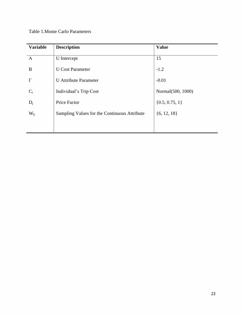
In this experiment, true parameters are assumed for individuals’ price and attribute

parameters in their indirect utility function for the outcome of interest, as well as distributions for

individuals’ costs, disturbances on the utility function, and reservation utilities (Table 1). These

values were all chosen as being reasonably representative of the dataset described below. The

utility parameters and trip cost are used to describe a particular individual. The cost factor and

attribute levels describe the points used in sampling.

Using these values draw a sample of n participants. For each participant, we calculate a

reservation utility, ( ), as well as a utility level for each combination of sampling Dj and

Wk:

where Ui,j,k is the level of utility associated with a cost for the participant, Ci, a multiple of cost

for the observation, Dj, and a value for the continuous attribute for the observation, Wk. From

this we calculate 9 responses from a dichotomous choice experiment, with response variable

YDC;i,j,k = 1 if , and YDC;i,j,k = 0 otherwise. Using the response variable, cost, and

sampling variables we estimate a fixed effects logit model, estimate marginal willingness to pay

11

for the attribute WTPDC, and calculate the 95% confidence interval and standard error using a

parametric bootstrap method (Krinsky-Robb, 1986).

After calculating the WTPDC, we calculate the continuous response for to be modeled

with a Weibull model, YW; i, j, by solving for the value of Wk that satisfies for each

value of Dj:

Note that this will give us three observations, instead of the nine from the dichotomous choice

experiment. From these, a Weibull duration model is estimated and willingness to pay, WTPW

calculated as outlined above. Standard Errors for this estimate are calculated using the delta

method. This procedure is repeated 10,000 times for each value of n.

Figure 1 displays the results of this in terms of standard errors as a function of sample

size for both the dichotomous choice (WTPDC) and continuous (WTPW) estimates. Based on the

parameterization, the true WTP = 120. This shows that WTPW has consistently smaller standard

errors, but that the standard errors appear to converge as sample size increases.4 Note that at n =

20 WTPW is significantly greater than zero at the 95% level, while WTPDCdoes not achieve this

level of significance until 40 < n < 50. If we consider the “moderate” sample size of n = 100,

WTPWhas a standard error of about 9.5. WTPDCdoes not achieve this until n > 150. So if we

consider a typical sample range for this case WTPW would require a sample size one half to two

thirds that of WTPDC for a given level of precision.

4 In general, the ratio of standard errors rs, will converge to some c ≤ 1. In this case, c = .75. It achieves rs, > .74 at

around n = 200.

12

Application: Offshore Energy Production and Beach Tourism in Delaware

In an effort to reduce dependence on fossil fuels, many coastal areas have proposed

offshore wind projects as an alternative source of energy. An issue that arises in virtually all

cases where wind projects are under consideration is whether the presence of wind turbines

disfigures the natural seascape thereby causing harm to residents and reducing tourism. Offshore

wind projects may include more than 100 turbines, each over 400 feet tall within sight of the

shore. Oil platforms can already be seen just a mile off the Gulf of Mexico coast. This potential

disamenity effect is often provided as a reason for not proceeding with an offshore wind project.

The Cape Wind project in the Nantucket Sound off Cape Cod in Massachusetts is probably the

best known. It was delayed for over a decade due to objections of local residents to the way the

project would interrupt their ocean views. One option is to locate a project at a distance sufficient

to alleviate the disamenity; possibly over the horizon.

Unfortunately, moving turbines further away from shore increases the capital and

maintenance costs as the depths to the ocean floor increase and the increased distance requires

higher energy-delivery costs and could affect the strength of available wind current. This

research estimates the visual externality costs associated with the wind turbines and investigates

how these externality costs are diminished as turbines are placed further from the shore. An

offshore wind project was recently proposed in Delaware to some controversy. There was also

discussion around the same time to opening up the area for offshore oil exploration. Estimating

the impacts of these projects on visitors would be a useful contribution to the debate.

Ladenburg (2009) provides an overview of valuation literature on wind projects. The

issue of offshore wind projects and distance from shore in Delaware in particular was studied by

13

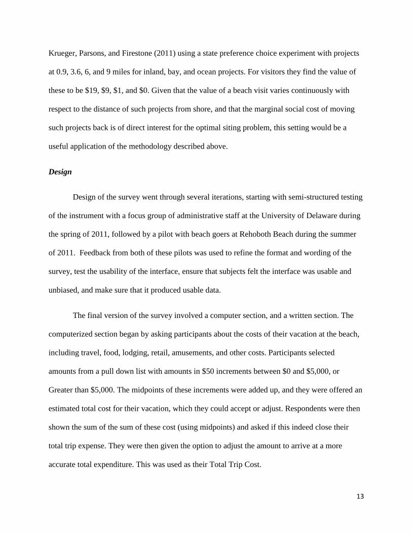
Krueger, Parsons, and Firestone (2011) using a state preference choice experiment with projects

at 0.9, 3.6, 6, and 9 miles for inland, bay, and ocean projects. For visitors they find the value of

these to be $19, $9, $1, and $0. Given that the value of a beach visit varies continuously with

respect to the distance of such projects from shore, and that the marginal social cost of moving

such projects back is of direct interest for the optimal siting problem, this setting would be a

useful application of the methodology described above.

Design

Design of the survey went through several iterations, starting with semi-structured testing

of the instrument with a focus group of administrative staff at the University of Delaware during

the spring of 2011, followed by a pilot with beach goers at Rehoboth Beach during the summer

of 2011. Feedback from both of these pilots was used to refine the format and wording of the

survey, test the usability of the interface, ensure that subjects felt the interface was usable and

unbiased, and make sure that it produced usable data.

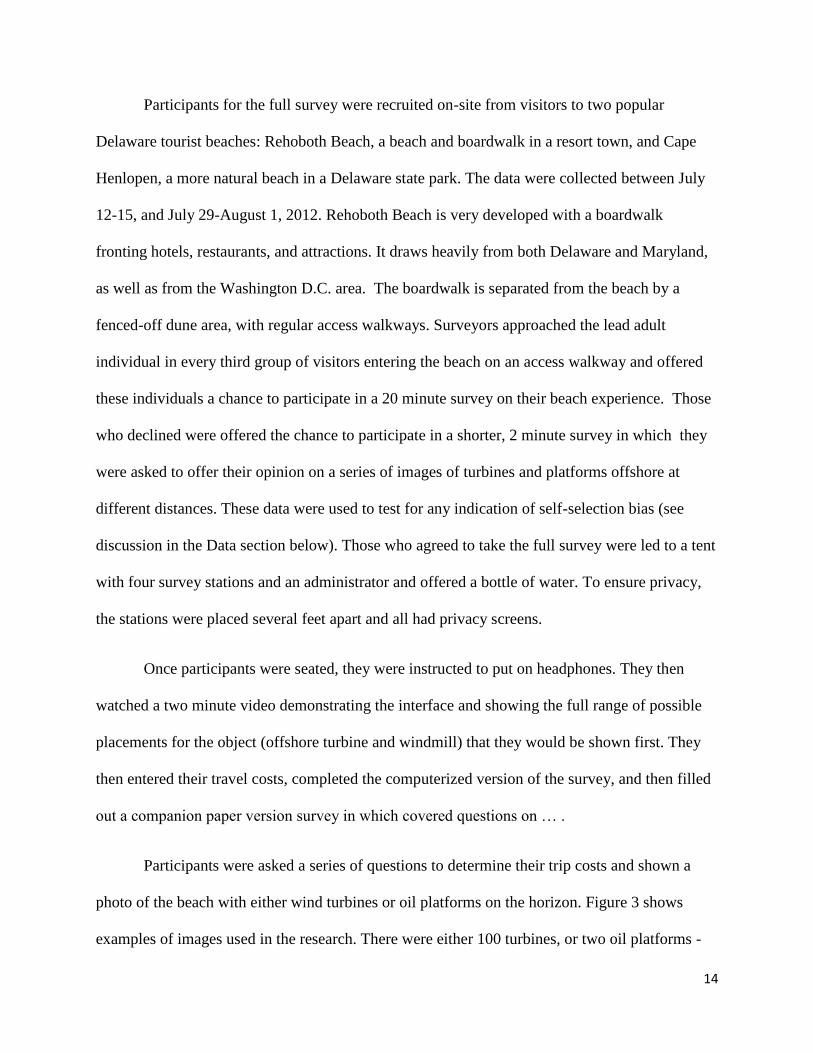
The final version of the survey involved a computer section, and a written section. The

computerized section began by asking participants about the costs of their vacation at the beach,

including travel, food, lodging, retail, amusements, and other costs. Participants selected

amounts from a pull down list with amounts in $50 increments between $0 and $5,000, or

Greater than $5,000. The midpoints of these increments were added up, and they were offered an

estimated total cost for their vacation, which they could accept or adjust. Respondents were then

shown the sum of the sum of these cost (using midpoints) and asked if this indeed close their

total trip expense. They were then given the option to adjust the amount to arrive at a more

accurate total expenditure. This was used as their Total Trip Cost.

14

Participants for the full survey were recruited on-site from visitors to two popular

Delaware tourist beaches: Rehoboth Beach, a beach and boardwalk in a resort town, and Cape

Henlopen, a more natural beach in a Delaware state park. The data were collected between July

12-15, and July 29-August 1, 2012. Rehoboth Beach is very developed with a boardwalk

fronting hotels, restaurants, and attractions. It draws heavily from both Delaware and Maryland,

as well as from the Washington D.C. area. The boardwalk is separated from the beach by a

fenced-off dune area, with regular access walkways. Surveyors approached the lead adult

individual in every third group of visitors entering the beach on an access walkway and offered

these individuals a chance to participate in a 20 minute survey on their beach experience. Those

who declined were offered the chance to participate in a shorter, 2 minute survey in which they

were asked to offer their opinion on a series of images of turbines and platforms offshore at

different distances. These data were used to test for any indication of self-selection bias (see

discussion in the Data section below). Those who agreed to take the full survey were led to a tent

with four survey stations and an administrator and offered a bottle of water. To ensure privacy,

the stations were placed several feet apart and all had privacy screens.

Once participants were seated, they were instructed to put on headphones. They then

watched a two minute video demonstrating the interface and showing the full range of possible

placements for the object (offshore turbine and windmill) that they would be shown first. They

then entered their travel costs, completed the computerized version of the survey, and then filled

out a companion paper version survey in which covered questions on … .

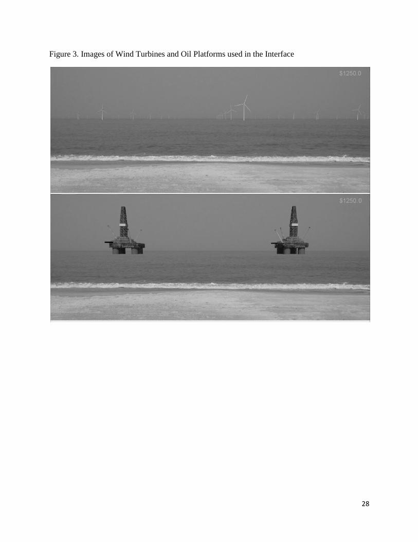
Participants were asked a series of questions to determine their trip costs and shown a

photo of the beach with either wind turbines or oil platforms on the horizon. Figure 3 shows

examples of images used in the research. There were either 100 turbines, or two oil platforms -

15

installations that would produce approximately the same amount of energy. Using buttons,

participants could scroll them in and out in intervals small enough as to be essentially continuous

(on the order of a couple feet). They could locate them anywhere between 10 miles, which is

about as far out as the turbines can still be seen on a average day, and .25 miles, which is as close

as they could come while still being mostly contained within the computer screen. They were

asked to use the computer interface to relocate the turbine/platform to the point at which they

would have not visited the beach. Then, they were then asked to imagine that, in order to

increase tourism after the construction of the project, the Chamber of Commerce offered travel

discounts that decreased their total trip cost. They were then asked to move the objects to a new

distance consistent with the new discount level. This was repeated for a second discount, for a

total of three price level observations per object, per participant. The possible discount rates were

(.25, .37, .48, .58, .67, .75, .82, .88, .93, .97). Two discounts were drawn at random without

replacement, and the higher discount was offered first. Participants would complete this process

for one type of project and then do the same for the other installation type. The type of

installation (wind turbines or oil platforms) shown first was alternated each day. The same

discounts were applied for wind turbines and oil platforms.

Following the computer survey participants were asked to complete a paper survey (see

Appendix) requesting demographic information. The last 13 questions were drawn from The

New Environmental Paradigm survey developed by environmental psychologists Schultz and

Zelensky (1999) for measuring environmental attitudes. These are listed in Table 3.

Results

16

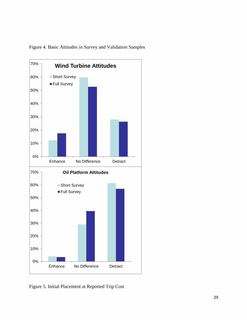
The sample included both a full study, and an abridged survey to test against the full

study for sample validity. The full study was in the form of a choice experiment conducted using

a computer interface that allowed participants to adjust the placement of wind turbines and oil

platforms relative to the beach. Both the full survey and the abridged validation survey were

shown wind turbines and oil platforms at random distances and were asked if they would have

enhanced, detracted, or made no difference to their experience. Figure 4 displays the results from

these. The distributions of attitudes look similar between the two samples, and are not

statistically different across samples.

Figure 5 shows the initial placement of both the turbine and oil platform projects. Note

that both have a spike at ten miles. This indicates censoring, as this is as far as the software

allowed them to push them back. It is a significant amount for both projects, but much larger

(about 50 versus 20 out of 224) for the oil platforms. For the uncensored observations, the oil

platforms are fairly uniformly distributed throughout the remaining range, while the turbines are

largely clustered below 3 miles - a result that is consistent with Krueger, Parsons, and Firestone

(2011).

Figures 6 and 7 display non-parametric hazard (representing the relative probability of

switching to an alternate travel destination at a given distance), and Kaplan-Meier survival

(representing the proportion of the population continuing to visit the beach at a given distance)

curves. The curves show a greater hazard and smaller surviving beach visiting population for the

oil platforms than the wind turbines. They also again illustrate dramatic increase in attrition

around 2-3 miles from shore.

17

The full duration model, since we have multiple dependent spell observations per subject,

is estimated as an Andersen-Gill multiple sequential event model (1982). This includes several

demographic controls, as well as the 4 factors obtained from a principle factor decomposition of

the thirteen New Environmental Paradigm questions. These results are displayed in Table 4. The

absolute value of the intercepts represent a baseline distance from shore, so that setting

everything else to 0, the wind turbines would be about 7 miles off shore, while the oil platforms

would be 13 miles (just over the horizon). These coefficients can be interpreted as a marginal

movement towards the shore, away from the horizon, in miles. For instance, the coefficient of

0.028 on percent trip discount implies that a percentage point increase in the trip discount would

be associated with a 0.028 mile movement towards the shore. The factors are specified on a 1 to

5 agree/disagree scale, so a unit change represents a step increase along one of those factors.

Finally, Figure 8 displays the total surplus of a beach trip with either wind turbines or oil

platforms on the horizon for the mean beach visitor. Note that the distance intersections at about

3 and 6 miles indicate that point at which such a visitor would choose a different vacation option

instead of visiting the beach. While the two curves appear to converge at the beach, this is not a

necessary outcome of the model, but indicate that the data suggest that once the installations get

close enough turbines and platforms are equally bad, however the disamenity is ameliorated with

distance much more quickly for the turbines.

Conclusions

This research proposed a new approach to valuing some non-market goods by taking

advantage of continuous variation in attributes of those goods. When data can be effectively

elicited in this way it has the advantage of more precise observations than are typically available

18

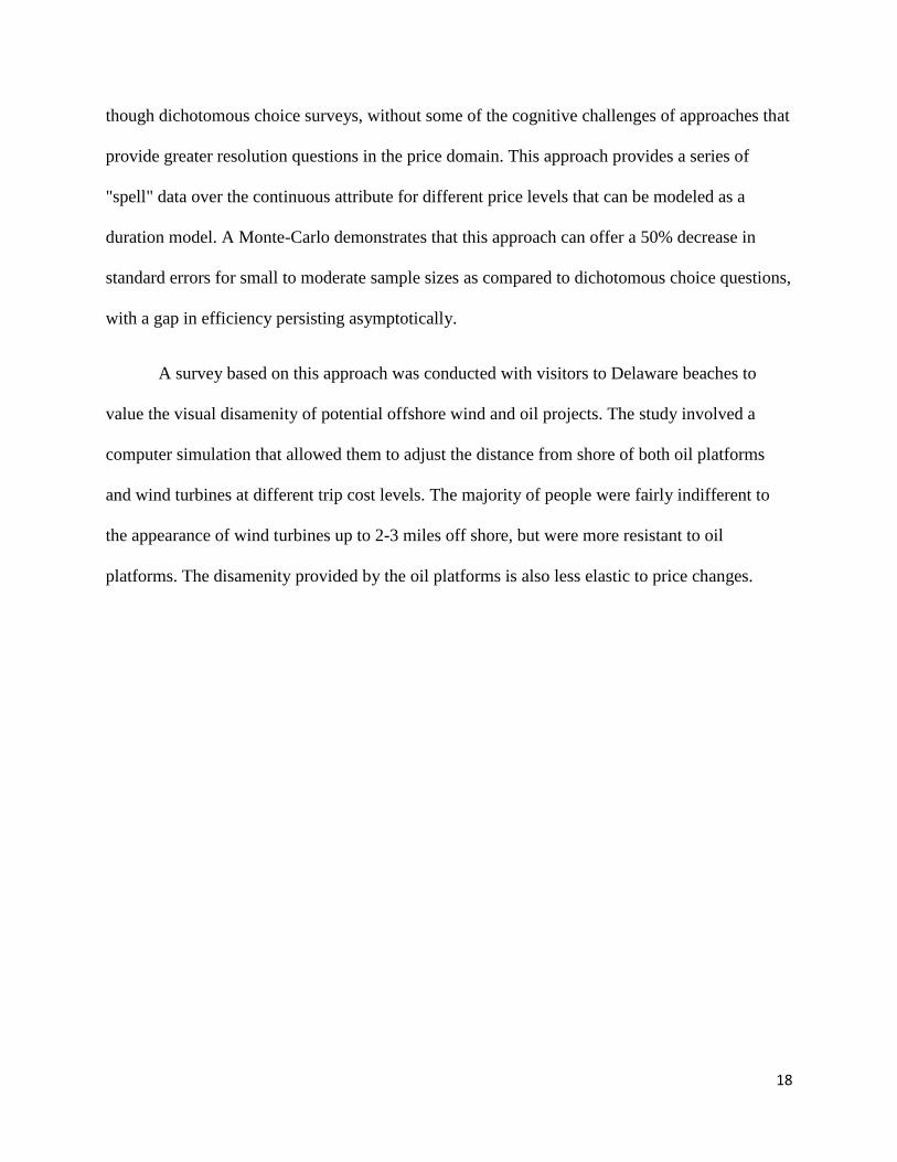
though dichotomous choice surveys, without some of the cognitive challenges of approaches that

provide greater resolution questions in the price domain. This approach provides a series of

"spell" data over the continuous attribute for different price levels that can be modeled as a

duration model. A Monte-Carlo demonstrates that this approach can offer a 50% decrease in

standard errors for small to moderate sample sizes as compared to dichotomous choice questions,

with a gap in efficiency persisting asymptotically.

A survey based on this approach was conducted with visitors to Delaware beaches to

value the visual disamenity of potential offshore wind and oil projects. The study involved a

computer simulation that allowed them to adjust the distance from shore of both oil platforms

and wind turbines at different trip cost levels. The majority of people were fairly indifferent to

the appearance of wind turbines up to 2-3 miles off shore, but were more resistant to oil

platforms. The disamenity provided by the oil platforms is also less elastic to price changes.

19

References

Alberini, .A 1995. Efficiency vs. Bias of WTP Estimates: Bivariate and Interval-Data Models.

Journal of Environmental Economics and Management 29:169-180.

Andersen, P.; Gill, R. (1982). "Cox's regression model for counting processes, a large sample

study.". Annals of Statistics 10 (4): 1100–1120.

Arrow, K., R. Solow, P. R. Portney, E. E. Learner, R. Radner, and H. Schuman, "Report of the

NOAA Panel on Contingent Valuation," Federal Register 58:10 (Jan. 15, 1993), 4601-

4614.

Balistreri, E., G. McClelland, G.L. Poe and W.D. Schulze, 2001. Can Hypothetical Questions

Reveal True Values? A Laboratory Comparison of Dichotomous Choice and Open-Ended

Contingent Values with Auction Values. Environmental and Resource Economics

18(3):275-292.

Borchers, Allison M. and Joshua M. Duke. 2012. Capitalization and proximity to agricultural and

natural lands: Evidence from Delaware. Journal of Environmental Management 99:110-

117.

Cameron, T.A., J. Quiggin. 1994. Estimation Using Contingent Valuation Data from a

"Dichotomous Choice with Follow-Up" Questionnaire. Journal of Environmental

Economics and Management 27(3):218-234.

Hanemann, M., J. Loomis, and B. Kanninen. 1991. Statistical Efficiency of Double-Bounded

Dichotomous Choice Contingent Valuation. American Journal of Agricultural Economics

73(4): 1255-1263.

20

Krinsky, I., and A.L. Robb. 1986. On Approximating the Statistical Properties of Elasticities.

The Review of Economics and Statistics 68(4): 715-719

Krueger, A.D., G.R. Parsons, and J. Firestone. 2011.Valuing the Visual Disamenity of Offshore

Wind Projects at Varying Distances from the Shore. Land Economics 87(2): 268-283.

Ladenburg, J. 2009. Stated Public Preferences for On-Land and Offshore Wind Power

Generation: A Review. Wind Energy 12(2): 171–81.

Lusk, J.L. and B. Norwood. 2005. Effect of Experimental Design on Choice-Based Conjoint

Valuation Estimates. American Journal of Agricultural Economics. 87:771-785.

Mataria A, S. Luchini, Y. Daoud, J.P. Moatti. 2007. Demand assessment and price-elasticity

estimation of quality-improved primary health care in Palestine: a contribution from the

contingent valuation method. Health Economics 16(10):1051-68.

Messer, K. 2009? Some presentation on arsenic water. Annual Meeting of the Economic

Sciences Associate, Tucson, AZ.

Plott, C. R. 1996.Rational Individual Behavior in Markets and Social Choice Processes: The

Discovered Preference Hypothesis, in Rational Foundations of Economic Behavior. K.

Arrow, E. Colombatto, M. Perleman, and C. Schmidt, eds. London: Macmillan and NY:

St. Martin’s, pp. 225–50.

Popkin, J.H., J.M. Duke, A.M. Borchers, T. Ilvento. Forthcoming. Social costs from proximity to

hydraulic fracturing in New York State. Energy Policy.

Steinberg, D. and R. Carson.1989. Demand Curve Estimation Via Survival Analysis. presented

at the Winter Conference, American Statistical Association, January 1989, San Diego.

21

Parsons, G.R., M.K. Hidrue, Z. Chen, N. Standing, and J. Lilley. 2013. Valuing Beach Width for

Recreational Use Combining Revealed and Stated Preference Data. Marine Resource

Economics.

Schultz, P.W., L. Zelezny. 1999. Values As Predictors Of Environmental Attitudes: Evidence

For Consistency Across 14 Countries. Journal of Environmental Psychology. 19(3): 255-

265

Wang, H., He, J. 2011. Estimating individual valuation distributions with multiple bounded

discrete choice data. Applied Economics. 43:21.

22

Table 1.Monte Carlo Parameters

Variable Description Value

Α U Intercept 15

Β U Cost Parameter -1.2

Γ U Attribute Parameter -0.01

Ci Individual’s Trip Cost Normal(500, 1000)

Dj Price Factor {0.5, 0.75, 1}

Wk Sampling Values for the Continuous Attribute {6, 12, 18}

23

Table 2. Descriptive Statistics

Sample Means of Participant Characteristics

Rehoboth Cape Henlopen

Sample Size 126 98

Age

43

49

Income (Median) $55,001-$65,000

$55,001-$65,000

Percent Male 50.8

44.9

Total Trip Cost 996

416

Initial Impression (at random distance from shore)

Wind Turbines

Enhance 0.143

0.143

No difference 0.508

0.408

Detract - Would still visit 0.206

0.265

Detract - Would not still visit 0.143

0.184

Initial placement (miles from shore) 2.52

3.06

Oil Platforms

Enhance 0.063

0.102

No difference 0.525

0.470

Detract - Would still visit 0.254

0.265

Detract - Would not visit 0.158

0.163

Initial placement (miles from shore) 5.87 5.89

24

Table 3. New Environmental Paradigm Factors

1. When humans interfere with nature it often

produces disastrous consequences.

8. The so-called "ecological crisis" facing

humankind has been greatly exaggerated.

2. Human ingenuity will insure that we do

NOT make the earth unlivable.

9. The earth is like a spaceship with very limited

room and resources.

3. Humans are severely abusing the

environment.

10. Humans were meant to rule over the rest of

nature.

4. The earth has plenty of natural resources if

we just learn how to develop them.

11. The balance of nature is very delicate and easily

upset.

5. Plants and animals have as much right as

humans to exist.

12. Humans will eventually learn enough about how

nature works to be able to control it.

6. The balance of nature is strong enough to

cope with the impacts of modern industrial

nations.

13. If things continue on their present course, we

will soon experience a major ecological catastrophe.

7. Despite our special abilities humans are still

subject to the laws of nature.

Factor 1 Factor 2 Factor 3 Factor 4

Agree Disagree Agree Disagree Agree Disagree Agree Disagree

3

5

13

8

10

2

4

6

8

12

1 1

3

5

9

11

6 12 5

7

25

Table 4. Anderson-Gill/Weibull AFT Regression

Miles from horizon (β>0 implies closer to shore)

N = 224

Wind Turbines Oil Platforms

C -7.111*** -13.029***

Percent Trip Discount 0.028*** 0.019**

Factor 1 0.315** 1.542***

Factor 2 -0.583*** -1.094***

Factor 2 0.321** -1.198*

Factor 4 0.318*** -1.485*

Primarily Water Activities 0.171 -0.757

Primarily Sand Activities -0.516 2.717***

Own Property at DE Beaches 1.339*** 5.148***

Income ($10,000) -0.035*** 0.182***

Age 0.150*** 0.110***

Male -0.696** -1.064*

Trip Cost ($100) -0.040*** 0.132**

Turbines First 0.719*** -1.990**

Henlopen -0.261 2.673***

Note: *,**,*** represent significance at the 10%, 5%, and 1% level. Controls for survey recruiter and

day were included but are not reported.

26

Figure 1. Results of Monte-Carlo Experiment

0

10

20

30

40

50

60

70

80

0 20 40 60 80 100 120 140 160

Stan

dar

d E

rro

r

Number of Participants (n)

S.E. for Estimated Average Marginal WTP (Population Average mWTP = 120)

Logit Model

Weibull Model

27

Figure 2. Map of Survey Sites

28

Figure 3. Images of Wind Turbines and Oil Platforms used in the Interface

29

Figure 4. Basic Attitudes in Survey and Validation Samples

Figure 5. Initial Placement at Reported Trip Cost

0%

10%

20%

30%

40%

50%

60%

70%

Enhance No Difference Detract

Wind Turbine Attitudes

Short Survey

Full Survey

0%

10%

20%

30%

40%

50%

60%

70%

Enhance No Difference Detract

Oil Platform Attitudes

Short Survey

Full Survey

30

0

10

20

30

40

50

60

Initial Platform Placement (in Miles from Shore)

0

10

20

30

40

50

60

Initial Turbine Placement (in Miles from Shore)

31

Figure 6. Average Smoothed Hazard Functions at Reported Trip Cost

Figure 7. Kaplan-Meier Survival Curves at Reported Trip Cost

32

Figure 8. WTP as a Function of Distance

33

Appendix: Paper Survey Date: __________

Subject #:_______

An Analysis of Offshore View Disamenities

Please answer the following questions.Your responses will be kept confidential. Please do not put your name

on any of the materials. Any questions may be addressed to the study administrator.

1. Please indicate your sex.

_______M ________F

2. In what year were you born?______________

3. What is the zip code at your primary residence? _________

4. How would you describe your area of residence?

_______Urban ________ Suburban________Rural

5. How years of formally schooling do you have? (Completed high school = 12 years)?__________

6. Are you currently…?

_______Employed Full Time ________Employed Part Time _______Self Employed

_______ Student ________ Homemaker _______ Retired

_______ Unemployed

7. What is your total household gross annualincome?

_______ Less than$25,000 _______ $95,001-$105,000 _______ $175,001-$185,000

_______ $25,001-$35,000 _______ $105,001-$115,000 _______ $185,001-$195,000

_______ $35,001-$45,000 _______ $115,001-$125,000 _______ $195,001-$205,000

_______ $45,001-$55,000 _______ $125,001-$135,000 _______ $205,001-$215,000

_______ $55,001-$65,000 _______ $135,001-$145,000 _______ $215,001-$225,000

_______ $65,001-$75,000 _______ $145,001-$155,000 _______ $225,001-$235,000

_______ $75,001-$85,000 _______ $155,001-$165,000 _______ Greater than $235,000

_______ $85,001-$95,000 _______ $165,001-$175,000 _______ Prefer not to say

8. Do you own property in a Delaware beach community (within 5 miles of an ocean beach)? (Exclude

investment properties)

_______Yes, my primary residence

Yes, my secondary residence

________No

9. Which activities are most important to you when visiting anocean beach or beach community in

Delaware? (If you engage or more than one, pick the one that is most important.)

_______Activities in or on the water

_______Activities on the sand

34

_______Activities at the boardwalk or in town

10. Are you staying here for more than one night on your current trip?(Please skip if your primary

residence in a Delaware beach community)

_______Yes ________No

-If yes, for how many nights are you staying? _______

11. How many hours do you expect to spend on the beach and boardwalk today? ________

12. Including yourself how many people are you traveling with? ________

- How many children under age 18? _______

13. How many days have you spent on Delaware’s ocean beaches(including time on the beach as well as

in the community)since Memorial Day?(Please skip if your primary residence in a Delaware beach

community)

14.

(Days on the beach since May 28th)? _______

15. How many more days do you expect to spend on Delaware’s ocean beaches before Labor Day

(Day on the beach between now and Sept. 3th)? _______

16. Are these primarily day trips or overnight trips?

_______ Day _______ Overnight

17. How many years have you been coming to Delaware’s ocean beaches? _______

18. What would you most likely do with your time if the beach you were visiting on your current trip was

closed for some reason for an extended period of time?

Visit another beach in Delaware

_______ Visit the same beach community in Delaware but not go on the beach

_______ Visit a beach in Maryland

_______ Visit a beach in Virginia

_______ Visit a beach in New Jersey

_______ Visit a beach outside the mid-Atlantic (not MD, VA, NJ pr DE)

_______ Visit a bay beach in Delaware

_______ Engage in some other non-beach recreation

_______ Stay home

_______Other: _______________________________

19. On a scale of 1 to 5, how favorable are you toward the development offshore wind power in the

Mid-Atlantic region?

20. On a scale of 1 to 5, how favorable are you toward the development of offshore oil production in the

Mid-Atlantic region?

35

Rank your level of agreement with each of the following statements

based on the this scale: STRONGLY MILDLY MILDLY STRONGLY AGREE AGREE UNSURE DISAGREE DISAGREE

20. How aware are you of the proposed wind farms off the coast of Delaware?

1 2 3 4 5

21. How aware are you of oil drilling regulations on the Atlantic Outer Continental Shelf ?

1 2 3 4 5

22. Wind power is a financially viable energy source for our country.

1 2 3 4 5

23. Offshore oil is a financially viable energy source for our country.

1 2 3 4 5

24. Wind turbines have a negative impact on the landscape.

1 2 3 4 5

25. Offshore oil platforms have a negative impact on the landscape.

1 2 3 4 5

26. When humans interfere with nature it often produces disastrous consequences.

1 2 3 4 5

27. Human ingenuity will insure that we do NOT make the earth unlivable.

1 2 3 4 5

28. Humans are severely abusing the environment. 1 2 3 4 5

29. The earth has plenty of natural resources if we just learn how to develop them.

1 2 3 4 5

30. Plants and animals have as much right as humans to exist.

1 2 3 4 5

31. The balance of nature is strong enough to cope with the impacts of modern industrial nations.

1 2 3 4 5

32. Despite our special abilities humans are still subject to the laws of nature.

1 2 3 4 5

33. The so-called "ecological crisis" facing humankind has been greatly exaggerated.

1 2 3 4 5

34. The earth is like a spaceship with very limited room and resources.

1 2 3 4 5

35. Humans were meant to rule over the rest of nature. 1 2 3 4 5

36. The balance of nature is very delicate and easily upset. 1 2 3 4 5

37. Humans will eventually learn enough about how nature works to be able to control it.

1 2 3 4 5

38. If things continue on their present course, we will soon experience a major ecological catastrophe.

1 2 3 4 5