The Deciduous Forest By: Kelli Ferguson Leah Holleman Jessica Corn.

Doppler Radar Wind Profiles
Iwan Holleman
Scientific Report, KNMI WR-2003-02, 2003

2

Contents
1 Introduction 5
2 Settings of Doppler Radar 92.1 Doppler Effect 92.2 Coherent Receiver 102.3 Doppler Power Spectrum 122.4 Clutter Filtering 152.5 Pulse-Pair Processing 172.6 Doppler Radar Scan Strategy 18
3 Methods for Wind Profile Retrieval 253.1 Radial Velocity from Local Wind Model 253.2 Velocity Azimuth Display 283.3 Volume Velocity Processing 303.4 Sources of Error 323.5 Implementation 34
4 Intercomparison of Wind Profile Retrieval Techniques 374.1 Available Wind Profile Data 374.2 Doppler Wind Profiles against Radiosonde 384.3 Doppler Wind Profiles against Hirlam 424.4 Rejection of Radial Velocity Outliers 44
5 Performance of VVP Retrieval Technique 475.1 Availability of Wind Profiles 475.2 Quality as a function of Wind Speed 495.3 Quality as a function of Height 515.4 Removal of Elevations 585.5 Outliers: Bird Migration? 60
6 Conclusions and Recommendations 65

4 CONTENTS
References 69

Chapter 1
Introduction
Upper-air wind observations are of crucial importance for general (operational) meteorology,nowcasting, aviation meteorology, and numerical weather prediction. On the synoptic scaledynamical weather phenomena are mainly determined by the wind field aloft, and on themesoscale the degree of organization of thunderstorms is determined by the vertical wind shearand helicity (Holton, 1992). In the WMO guide on Meteorological Instruments and Methodsof Observation, a chapter has been dedicated to measurement of upper-air wind (WMO, 1996).Furthermore, the importance of upper-air wind forces many meteorological institutes to launchradiowind sondes, designated to measure upper-air wind only, in between the radiosonde ob-servations.
Apart from radiowind or radiosonde, many other (remote sensing) techniques are availableto measure the upper-air wind. Observations by ascending, descending, and cruising airplanes,AMDARs, are nowadays a valuable source of upper-air wind data. Ground-based remote sens-ing techniques for observation of wind profiles, like sodar, wind profiler, and lidars, are usedoperationally or are being developed for operational use. Satellite systems can be used forupper-air wind observations as well. Cloud-motion vectors, a measure for upper-air wind, arededuced from sequences of infrared images from the geostationary Meteosat and assimilatedin operational Numerical Weather Prediction (NWP) models. In addition, ESA has plannedan Atmospheric Dynamics Mission (ADM) which will be launched in 2006 and will measurewind profiles using the lidar technique.
At KNMI scientific work focused on several of these techniques for obtaining upper-airwind data is ongoing. The Quality Evaluation Centre (QEvC) for E-AMDAR observationsis hosted by KNMI and quarterly reports on quality and availability of the observations areproduced (Meulen, 2003). At the Cabauw remote sensing site, a boundary layer wind profileris stationed and a long-term intercomparison with tower measurements has been performed byKlein Baltink (1998). The potential impact of a network of boundary layer wind profilers andsodars for mesoscale wind analysis in the Netherlands has been assessed by the ASWAN project(Tijm and Wu, 2000). Dlhopolsky and Feijt (2003) have investigated the representative heights

6 Introduction
for atmospheric motion vectors deduced from Meteosat. KNMI takes part in the developmentof ADM and Observation System Simulation Experiments (OSSEs) are performed by Marseilleand Stoffelen (2003).
Doppler weather radars are also capable of providing upper air wind observations usingdedicated methods for retrieval of wind profiles. In the early sixties, Lhermitte and Atlas (1961)and Browning and Wexler (1968) introduced the Velocity-Azimuth Display (VAD) techniquefor the extraction of upper-air wind data from Doppler radar observations. When using theVAD technique, it is not possible to separate the contributions of the vertical velocity, which isa sum of the vertical wind velocity and the hydrometeor fall velocity, and the divergence of thehorizontal wind field to the offset of the VAD. Improved versions of the VAD technique, whichare mainly designed to separate these two contributions, were developed in the late eighties andearly nineties and have been dubbed the Extended-VAD (EVAD) technique (Srivastava et al.,1986; Matejka and Srivastava, 1991) and the Concurrent-Extended-VAD (CEVAD) technique(Matejka, 1993). Instead of processing a single VAD or a series of VADs, one can also processall available volume scan data in a certain height layer at once using a multi-dimensional linearregression. This so-called Volume Velocity Processing technique (VVP) has been introducedby Waldteufel and Corbin (1979). Nowadays, both the VAD technique and the VVP techniqueare widely used to retrieve wind profiles from Doppler radar observations.
Despite the widespread use of the VAD and VVP retrieval techniques, only a few veri-fication or case studies with the retrieved wind profiles have been published so far and nointercomparison study between VAD and VVP retrieved horizontal wind data has been pub-lished up to now. Andersson (1998) has published verification results of VAD wind profilesagainst those from radiosonde and the Hirlam model. Both the availability and the accuracyof the VAD wind vectors of the Swedish weather radars were investigated. The availability ofthe VAD wind vectors is about 80% at 925 hPa, and it drops to about 15% at 400 hPa. Therms vector differences between the VAD wind vectors and the radiosonde wind vectors is about3 m/s. The EVAD technique has been used to study the trailing anvil region associated witha squall line (Srivastava et al., 1986). Profiles of wind speed and direction, hydrometeor fallspeed, and divergence have been obtained. Details of the kinematic structure of the mid-latitudesquall line are revealed by this Doppler radar study. Xin and Reuter (1998) have investigatedhow the number of VVP parameters affects the accuracy of the retrieved parameters and haveapplied the optimized VVP technique to an Alberta storm. It is concluded that the initiationand enhancement of precipitating cells were associated with the VVP low-level convergence.An interesting intercomparison of divergence and vertical velocity obtained by (C)EVAD, andVVP techniques is presented by Cifelli et al. (1996). The performance of the techniques werequite similar, although the VVP profiles often extended to greater heights. Unfortunately, nointercomparison of the retrieved wind speeds and directions was made. Boccippio (1995) hasperformed a diagnostic analysis of the VVP retrieval technique and he has developed an algo-rithm for preparation and analysis of a robust VVP retrieval.
An important application of (Doppler radar) wind profiles is the assimilation in operational

Introduction 7
NWP models. The European Union COST-717 program on “Use of radar observations in hy-drological and NWP models” deals amongst other things with quality control and assimilationof Doppler radar wind profiles and radial velocity data in NWP models (Rossa, 2000). Aspart of this program, Lindskog et al. (2002) have compared the relative impact of assimilatingVAD-wind profiles and radial wind super-observations in the Hirlam model. The benefits tothe model forecast were found to be comparable for both types of wind information. At the Na-tional Centers for Environmental Prediction (NCEP) assimilation of VAD wind profiles fromthe WSR-88D radars started in 1997, but soon many problems with the data became evident andthe operational assimilation was ended in 1999 (Collins, 2001). A quality control procedure forVAD profiles has been developed which removes wind vectors with very small magnitude, clearoutliers, and “wind” vectors due to migrating birds. The VAD profiles were re-admitted oper-ationally in 2000 (Collins, 2001). Within the framework of the Eumetnet WINPROF programon wind profilers, a wind profile database and quality control center (CWINDE) is operatedby the UK Met Office (CWINDE, 2003). Both wind profiler and Doppler radar wind profilesare collected and processed by the CWINDE hub. The quality control is performed by a veri-fication against the UK regional model. Monthly reports on the availability and quality of theprofiles are produced for all sites sending data to the hub.
In this scientific report, an intercomparison of different implementations of the VAD andVVP retrieval techniques and an extensive verification of Doppler radar VVP wind profilesagainst radiosonde and Hirlam model profiles are presented. Nine months of wind profile datahave been used for the intercomparison and verification. Modules to retrieve wind profiles fromDoppler volume scan data using different implementations of the VAD and VVP techniqueshave been developed, but wind profiles from the Rainbow VVP module (Gematronik, 2003)have been considered as well. It is concluded that the VVP retrieval technique provides windprofiles with a higher availability and a better quality than the VAD technique. In addition,it is found that the most simple implementation of the VVP technique, i.e., with the fewestwind field parameters, provides the best horizontal wind data. The verification results indicatethat the accuracy of the VVP wind profiles generally satisfies the requirements for upper-airwind measurements as provided by WMO (1996). Recommendations for improvement of theRainbow VVP module (Gematronik, 2003) which will be used operationally at KNMI aremade. The outline of the remaining of the report is as follows:
• In chapter 2 an introduction to Doppler radar velocity measurements is given and therelevant settings of the Doppler radar system are discussed. In addition, a couple of ex-periments are presented which aided in finalizing the settings of the Doppler processing.
• The basic principles behind the Doppler radar wind profile retrieval techniques are intro-duced in chapter 3. The VAD and VVP retrieval techniques are described and differentimplementations of the techniques are discussed.
• In chapter 4 the results from the intercomparison of VAD and VVP retrieval techniquesand the different implementations are presented.

8 Introduction
• An extensive evaluation of the performance of the VVP retrieval technique is presented inchapter 5. Both the availability and the quality of the retrieved wind vectors are analyzedand discussed in detail.
• In the last chapter the conclusions from the intercomparison and verification are summa-rized and recommendations for further application are made.

Chapter 2
Settings of Doppler Radar
2.1 Doppler EffectA Doppler weather radar is capable of determining one component of the velocity of scatter-ing particles. Only the velocity component along the line of sight, the so-called radial ve-locity, can be determined. A Doppler radar is commonly associated with measurements offrequency shifts, because of the low velocities of hydrometeors, however, these shifts cannotbe observed directly. The phase of the scattered electromagnetic waves is employed to deter-mine the Doppler frequency shift instead. The received phase φ from an electromagnetic wavescattered at range R from the radar is given by:
φ = 2π2R
λ(2.1)
where λ is the wavelength of the electromagnetic waves. The Doppler frequency shift fd isrelated to the rate of phase change:
fd =1
2π
dφ
dt=
2Vrλ
(2.2)
where the radial velocity Vr is defined as the derivative of the range with respect to time. Thisequation for the Doppler frequency shift can also be deduced by applying the classical Dopplereffect to scattering from a moving target. For a hydrometeor with a radial velocity of 10 m/sobserved with a C-band radar (λ = 5.3 cm), the Doppler frequency shift is roughly 400 Hzwhich is about seven orders of magnitude smaller than the radar frequency.
A pulsed Doppler radar transmits a sequence of electromagnetic pulses and receives thescattered signal in between. Typically the transmitted pulses have a power of 250 kW anda duration of 0.5 µs. Most operational Doppler radars transmit an equidistant sequence withseparation given by the pulse repetition time T , which is typically on the order of 1 ms. Foreach range bin, the phase of the received electromagnetic waves is monitored from pulse to

10 Settings of Doppler Radar
pulse. The difference between phases from two subsequent pulses ∆φ is directly related to theradial velocity:
∆φ = 2π2VrT
λ(2.3)
It will be detailed below that the retrieval of the (average) radial velocity and spectral widthfrom the received electromagnetic waves is not this straightforward, but this equation presentsthe basic principle. The maximum phase difference that can be determined unambiguously islimited to ±π, and therefore the radial velocity has a maximum unambiguous value as well.The maximum unambiguous radial velocity is given by:
V ur =
λ
4T=λ PRF
4(2.4)
where PRF is the Pulse Repetition Frequency. For a typical C-band Doppler radar using a pulserepetition time of 1 ms or equivalently a PRF of 1 kHz, the maximum unambiguous velocity isequal to 13 m/s.
2.2 Coherent ReceiverA pulsed Doppler weather radar can either be “fully coherent” or “coherent on receive”. In theformer case, the transmitter is based on a klystron and therefore the phase of each pulse canbe controlled. The WSR-88D weather radars in the NEXRAD network (Serafin and Wilson,2000), for example, are fully coherent. In the latter case, the transmitter is based on a magnetronand therefore the phase of each pulse is fully random. Most operational Doppler weatherradars in Europe, including those of KNMI, are coherent on receive (Meischner et al., 1997).A klystron-based receiver is more expensive, but offers higher (phase) stability and reliability.On the other hand, a magnetron-based radar has hardly any problems with second-trip echoes(range aliasing) due to the incoherent nature of the transmitted pulses.
A simplified overview of a coherent on receive Doppler radar is depicted in figure 2.1.The transmitted pulses are generated by a magnetron and are fed into the radar antenna via atransmit-receive coupler. The phase of the transmitted pulse is monitored and used to start thestable local oscillator (STALO). The STALO provides two reference signals: one in phase withthe transmitted pulse and one 90 degrees out of phase. The received signal, or echo, E(t) canbe represented by:
E(t) = E(t) sin(ωt+ φ(t)) (2.5)
with E(t) the (time-dependent) amplitude of the echo, ω the angular frequency of the elec-tromagnetic wave, and φ(t) the phase shift with respect to the transmitted wave. An in-phasesignal I(t) and a quadrature signal Q(t) are generated by multiplying the received signal with

2.2 Coherent Receiver 11
Magnetron TR
STALO
ϕ
90 0
Ant
enna
X
X
I
Q
Figure 2.1: A simplified overview of a coherent on receive Doppler weather radar. The con-nections between the magnetron, transmit-receive coupler (T/R), antenna, stable local oscillator(STALO), and the down-converters (X) for the in-phase (I) and quadrature phase (Q) outputsare shown.
the in-phase (sin(ωt)) and out-of-phase (cos(ωt)) signals of the STALO, respectively, and aver-aging of the result over many wave cycles. In mathematical formulation this down-conversionprocess is described by:
I(t) ≡ ω
π
∫ 2π/ω
0E(t) sin(ωt) dt ' E(t) cosφ(t) (2.6)
Q(t) ≡ ω
π
∫ 2π/ω
0E(t) cos(ωt) dt ' E(t) sinφ(t) (2.7)
It is evident that the amplitude and phase of the echo can be deduced from the in-phase andquadrature-phase signals. The averaging period depends on the desired range resolution, but istypical on the order of 1 µs. For weather echoes, the I(t) andQ(t) signals are uncorrelated andhave a Gaussian distribution (Doviak and Zrnic, 1993).
It has been detailed in the previous section that the radial velocity can be deduced from evo-

12 Settings of Doppler Radar
lution of the phase of the received signal during subsequent pulses. The in-phase and quadraturephase signals contain information on this phase evolution. The time coordinate of the I(t) andQ(t) signals is primarily related to the range of the scatterers from the radar. After a time T ,equal to the pulse repetition time, the signals are primarily related to the echoes of the nexttransmitted pulse. During Doppler processing the I(t) and Q(t) signals are analyzed at con-stant range and sampled by each transmitted pulse. It is convenient to combine the I(t) andQ(t) signal to one complex quantity:
Z(n) ≡ I(nT ) + i Q(nT ) (2.8)
where Z(n) is the complex signal at a certain range for transmitted pulse n. During Dopplersignal processing a series of Z(n) values is analyzed for each range bin.
The evolution of the amplitude and phase of the complex signal as a function of pulsenumber is determined using autocorrelation. The autocorrelation function R(l) is calculatedfrom the complex signal Z(n):
R(l) ≡ 1
N − |l|N−|l|−1∑
n=0
Z?(n) Z(n + l) (2.9)
In this equation N represents the number of transmitted pulses used to calculate the autocor-relation function and l is the lag of the autocorrelation. For a lag l = 0 the autocorrelation isequal to the intensity of the received signal, while the autocorrelation for lags of 1 and 2 canbe used to extract the mean radial velocity and the spectral width. From the autocorrelation,the power spectrum S(f), also known as periodogram, can be obtained using a discrete Fouriertransform (DFT):
S(f) ≡ TN−1∑
l=−N+1
R(l) exp(−i2πlTf) (2.10)
From a signal processing point of view it is important to note that the power spectrum can alsobe obtained directly from the complex signal Z(n) using DFT (Doviak and Zrnic, 1993). Thefrequency axis of the power spectrum is proportional to the radial velocity and can directly beconverted using equation 2.2. The power spectrum of the received signal is a power-weighteddistribution of the radial velocities of the scatterers (Doviak and Zrnic, 1993). This “Dopplerspectrum” plays a key role in the understanding and processing of Doppler radar observations.
2.3 Doppler Power SpectrumThe Doppler spectrum or power spectrum contains the information on the distribution of radialvelocities of the meteorological scatterers in the power-weighted measurement volume. Fromthe shape of the Doppler spectrum, the hydrometeor parameters, most notably the mean radial

2.3 Doppler Power Spectrum 13
Figure 2.2: A typical Doppler spectrum for a resolution volume within a thunderstorm. Thisspectrum is obtained from a Fourier transform using 64 samples and a von Hann window. Thisfigure is taken from Doviak and Zrnic (1993).
velocity and spectral width, can be deduced. In figure 2.2 an example of a Doppler spectrumfrom hydrometeor scatterers is depicted. It will be detailed below that the Doppler processingused at KNMI does not allow for extraction of the power spectrum, and therefore the figureis taken from Doviak and Zrnic (1993). The unambiguous velocity interval of this Dopplerspectrum is ±28.5 m/s and the received power for each velocity bin is given in decibel relativeto the peak power. The Doppler spectrum has a clear maximum around a velocity of 15 m/swhich is equal to the mean radial velocity. The spectral width of 2.2 m/s is determined from aGaussian fit to the power spectrum. In addition it is evident from the figure that the noise levelis about 25 dB below the peak power. Ground clutter, i.e., signal from fixed non-hydrometeortargets, can easily be recognized from a Doppler spectrum. An example of a Doppler spectrumof ground clutter is depicted in figure 2.3 which again is taken from Doviak and Zrnic (1993).It is obvious that ground clutter produces a narrow peak centered around zero velocity. Thespectral width of this clutter peak is only 0.45 m/s and it is thus a factor of four smaller thanthat of the hydrometeor peak.
For a Doppler weather radar at least three types of contributions to the power spectrum canbe distinguished: noise, ground clutter, and hydrometeor signal. The relative importance ofeach of these contributions depends on the range from the radar and the actual meteorologicalcircumstances. In order to process the received Doppler signal assumptions on the spectralshape of these contributions have to be made. For white noise the power spectrum is constant

14 Settings of Doppler Radar
Figure 2.3: A Doppler spectrum of ground clutter for an antenna scanning at 10 degree/s. TheDoppler processing is similar that of the data in figure 2.2. The ground clutter peak is centeredat zero velocity and its spectral width is only 0.45 m/s. This figure is taken from Doviak andZrnic (1993).
and equal to:
S(f) ≡ TN0 (2.11)
R(n) =
{N0 for n = 00 for n 6= 0
(2.12)
where N0 is the noise power. The corresponding autocorrelation function for white noise isobtained via an inverse discrete Fourier transform. The autocorrelation function is zero forn 6= 0 reflecting that white noise is completely uncorrelated. The power spectrum of a groundclutter signal can be approximated by a Gaussian function centered around zero frequency:
S(f) ≡ C0
σc√
2πexp(−f 2/(2σ2
c )) (2.13)
R(n) = C0 exp(−(2πnTσc)2/2) (2.14)
In these equations for the power spectrum and the autocorrelation function, C0 and σc representthe power and the spectral width, respectively, of the ground clutter signal. For a hydrometeor

2.4 Clutter Filtering 15
scattering signal, the power spectrum is well approximated by a Gaussian function centeredon the mean Doppler frequency shift fd. Using equation 2.2 this frequency shift can be con-verted to the mean radial velocity of the scattering hydrometeors. The power spectrum andautocorrelation function for the hydrometeor signal are described by:
S(f) ≡ S0
σ√
2πexp(−(f − fd)2/(2σ2)) (2.15)
R(n) = S0 exp(i2πnTfd) exp(−(2πnTσ)2/2) (2.16)
where S0 is the scattered power and σ is the spectral width. Any Doppler spectrum can bedescribed by a linear combination of the preceding contributions. As a matter of fact this alsoholds true for the autocorrelation functions, because the conversion between power spectral andautocorrelation is linear (DFT). It will be detailed below that this property of the autocorrelationfunction is employed during Doppler pulse-pair processing.
2.4 Clutter FilteringAs implied by its name clutter is an unwanted signal in Doppler radar observations of re-flectivity factor and mean velocity. Clutter may caused by scattering of the antenna sidelobepower from ground surface, by (partial) beam blockage, by anomalous propagation followedby scattering from ground or sea surface, or by scattering from non-hydrometeor scatterers inthe atmosphere. Clutter from ground targets, so-called ground clutter, is infamous for causingspurious echoes in weather radar reflectivity images, but it also affects the quality of meanradial velocity observations. Seltmann (2000) has shown that ground clutter superimposed ona hydrometeor signal leads to lower signal quality and a bias towards zero of the mean radialvelocity. Ground clutter interference in the Doppler signal Z(n) is suppressed, however, bydigital filtering in the time or frequency domain.
It has been shown in figure 2.3 that ground clutter gives rise to a narrow peak around zerofrequency in the Doppler spectrum. This low frequency component can be removed from theDoppler signal by applying a sharp high-pass filter. Digital filtering of the Doppler signal caneither be done in the frequency domain or in the time domain. In the former case the powerspectrum is calculated, subsequently a window function is applied, and finally the spectrumaround zero frequency is reconstructed using interpolation (Sigmet, 1998). In the latter casefiltered signal ˜Z(n) is given by:
Z(n) =M∑
m=0
bmZ(n−m)−M∑
m=1
cmZ(n−m) (2.17)
where M is the order of the time domain filter. It is evident that the filtered signal is a linearcombination of the (un)filtered signals at previous time steps. When all coefficients cm are

16 Settings of Doppler Radar
0.00 0.05 0.10 0.15 0.20 0.25 0.30 0.35 0.40 0.45
–50.0
–40.0
–30.0
–20.0
–10.0
0.0
Figure 2.4: Filter characteristics of digital Infinite Impulse Response high-pass clutter filterswith 40 dB attenuation. These filters are preprogrammed in the RVP6 signal processor. Thehorizontal axis represents the radial velocity scaled to the unambiguous velocity and the verticalaxis the attenuation in dB. This figure is taken from Sigmet (1998).

2.5 Pulse-Pair Processing 17
zero the filter is a so-called finite impulse response filter (FIR), and else it is a so-called infiniteimpulse response filter (IIR). More information on digital filtering in the time domain can befound in Press et al. (1992). The filter characteristics or filter function depends on the choiceof coefficients bm and cm.
The RVP6 Doppler Signal Processor (Sigmet Inc.) is shipped with fourteen sets of prepro-grammed coefficients for fourth-order IIR filtering: seven sets for 40 dB ground clutter sup-pressing and seven sets for 50 dB suppression (Sigmet, 1998). In figure 2.4 the filter functionsof the seven 40 dB clutter filters are depicted. The horizontal axis represents the frequency orradial velocity scaled to the unambiguous one and the vertical axis gives the suppression of thefilter in dB. It is evident that the cut-off frequency and “tail” of the seven high-pass filters aredifferent. The filter functions of the 50 dB clutter filters (not shown) have a much longer tailthan the corresponding 40 dB filters, which is the cost of the higher suppression. It is importantto note that, in contrast to frequency domain filtering, time domain filtering does not allow forreconstruction of the power spectrum around zero frequency. Given the higher computationaldemand for frequency domain filtering and the amount of Doppler data to be processed, ourcurrent signal processors can only handle time domain filtering.
2.5 Pulse-Pair Processing
The pulse-pair method is a widely used method for estimation of the mean radial velocity andspectral width of Doppler spectra in the time domain. One of the first articles that presentsan extensive description and analysis of the pulse-pair method is written by Srivastava et al.(1979). The pulse-pair method assumes that the noise is truly white and uncorrelated from thesignal. In addition, the method assumes that the power spectrum can be approximated by asingle Gaussian function. It is crucial that a possible ground clutter peak is removed from theDoppler signal by time or frequency domain filtering before pulse-pair processing is applied.The presence of ground clutter will result in a bias of the estimated mean radial velocity towardszero (Seltmann, 2000).
Assuming that the power spectrum consists of white noise and a single Gaussian functionfrom hydrometeor scattering, equations 2.12 and 2.16 can be used to calculate the approximateautocorrelation function at the zeroth, first, and second lags:
R(0) = S0 +N0 (2.18)R(1) = S0 exp(i2πTfd) exp(−(2πTσ)2/2) (2.19)R(2) = S0 exp(i4πTfd) exp(−2(2πTσ)2) (2.20)
The autocorrelation function at zeroth lag R(0) is equal to the received power and is in princi-ple only of importance for reflectivity factor measurements. The mean radial velocity can be

18 Settings of Doppler Radar
estimated from the autocorrelation function at the first lag:
Vr =λfd2
=λ
4πTarg(R(1)) (2.21)
It is important to note that this estimation of the mean radial velocity is unbiased by whitenoise and unbiased for symmetric Doppler spectra (Passarelli Jr. and Siggia, 1983). For highsignal-to-noise ratios (S0 � N0), the spectral width can be estimated using just the zeroth andfirst lag of the autocorrelation function. A more accurate approach is to use the autocorrelationfunction at the first and second lag to calculate the spectral width:
W =λσ
2=
λ
2π√
6T
√√√√ln
(|R(1)||R(2)|
)(2.22)
whereW is the spectral width in m/s. It has been detailed in section 2.2 that the autocorrelationfunction at a certain lag can be obtained from the received Doppler signal. By insertion of theobtained autocorrelation at zeroth, first, and second lags into the preceding equations, the meanradial velocity and the spectral width can be extracted from the received signal. This type ofpulse-pair processing is integrated in the RVP6 Doppler signal processors which are used atKNMI.
Apart from deriving the reflectivity factor, the mean radial velocity, and the spectral width,the RVP6 processor has the ability to accept or reject range bins based on threshold qualifiersderived from the received signal (Sigmet, 1998). The type of threshold qualifiers used for thequality control of the range bins depends on the output parameter. For mean radial velocity aSignal Quality Index and a Clutter Correction threshold can be applied, and for spectral widthan additional Weather Signal Power threshold is available. The Signal Quality Index (SQI) isdefined as the ratio of the autocorrelation at the zeroth and first lags:
SQI ≡ |R(1)|R(0)
=S0
N0 + S0
exp(−(4πTW )2/(2λ2)) (2.23)
and is always between zero and one. The SQI threshold qualifier is a combination of signal-to-noise ratio and spectral width and thus is a measure of the spectral brightness of the Dopplersignal. The Clutter Correction (CCOR) threshold is defined as the ratio of the autocorrelationfunction at lag zero after clutter filtering and that before filtering. The CCOR factor is givenin dB and is also used to correct the reflectivity signal from the LOG channel. Finally, theWeather Signal Power (SIG) is defined as the ratio (in dB) of signal power S0 and the noisepower N0.
2.6 Doppler Radar Scan StrategyKNMI operates two identical C-band Doppler weather radars. In this study volume data fromthe radar in De Bilt and processed wind profiles from both radars have been used. The De

2.6 Doppler Radar Scan Strategy 19
Table 2.1: Settings of De Bilt and Den Helder radars for dedicated Doppler scan. This scan isrepeated every 15 minutes and volume data of clutter corrected reflectivity factor, mean radialvelocity, and spectral width are stored.
Parameter ValueLow PRF 750 HzHigh PRF 1000 HzUnambiguous velocity 39.9 m/sMaximum range 140 kmRange bin size 0.5 kmAzimuthal speed 24 deg/sAzimuthal step 1 degNumber of elevations 10Elevations (deg) 0.5, 2, 3.5, 5, 7, 9, 12, ...(De Bilt only) 15, 20, 25
Bilt radar is located at a latitude of 52.10N and a longitude of 5.18E, and the antenna feed ismounted at a height of 44 m above mean sea level. The Den Helder radar is located at a latitudeof 52.96N and a longitude of 4.79E, and the antenna feed is mounted at a height of 51 m abovemean sea level. The Gematronik radars (Meteor AC360) have an antenna with a 4.2 m diameterand a beam width of about 1 degree. The peak power and width of the transmitted pulses are250 kW and 0.5 µs, respectively.
A dedicated Doppler volume scan has been defined on both radars (see table 2.1). ThisDoppler scan is repeated every 15 minutes and does not interfere with the operational reflectiv-ity scans, which consist of a 4 elevation scan every 5 minutes and a 14 elevation scan every 15minutes. For each scan the volume data of filtered reflectivity factor, mean radial velocity, andspectral width are stored. Unfortunately, the current radar processing system does not allow foradditional storage of the unfiltered reflectivity data. Availability of both the Doppler filteredand unfiltered reflectivity factor volume data would enable a fair comparison with the currentground clutter rejection scheme by Wessels and Beekhuis (1997). The unambiguous velocityrange of the Doppler scans is extended using the dual-PRF technique (Sirmans et al., 1976). Adiscussion on the properties and capabilities of the dual-PRF technique is beyond the scope ofthis report. An extensive analysis and a technique for correction of dual-PRF velocity data arepresented by Holleman and Beekhuis (2003).
The parameters defining the dedicated Doppler scan and corresponding values are displayedin table 2.1. The ratio between the low and high PRF has been set to 3 : 4 in order to extendto unambiguous velocity interval by a factor of 3. The absolute value of the PRFs is a balancebetween the unambiguous velocity and the maximum range. For wind profiling the maximum

20 Settings of Doppler Radar
0.0 0.2 0.4 0.6 0.8 1.0Signal Quality Index
0.0
0.1
0.2
0.3
0.4
0.5
Frac
tion
Valid pointsOutliers
0.0 0.2 0.4 0.6 0.8 1.0Signal Quality Index
0.0
0.5
1.0
1.5
2.0
2.5
Std
Dev
[m/s
]
Std Dev
Figure 2.5: The influence of the Signal Quality Index (SQI) threshold on the fraction of validrange bins, the fraction of velocity outliers, and the standard deviation of the velocity estimates.The fraction of outliers is given relative to the number of valid range bins. These data have beencollected on 13 September 2001.
range is not an issue, but this Doppler scan strategy has also been used for analyzing the dual-PRF technique (Holleman and Beekhuis, 2003). The range bin size is always a multiple of0.125 km and its lower limit is determined by the maximum number of range bins that can beprocessed in real-time (Sigmet, 1998). For a given set of PRFs, the azimuthal speed determinesthe number of transmitted pulses available for the pulse-pair processing. The azimuthal speedis determined, however, by the available time between the operational reflectivity scans. The 10elevations have been optimized for profiling up to an altitude of about 6 km. The three highestelevations are not allowed in Den Helder because of regulations from the nearby naval air base.
The default value for Clutter Correction (CCOR) qualifier threshold is −25 dB. To be onthe safe side, a CCOR threshold of−20 dB has been selected which will reject somewhat moreclutter range bins. For optimizing the Signal Quality Index (SQI), a series of measurementshas been performed on 13 September 2001. During the measurement period there were a fewscattered showers within range of the radar. The radial velocity data of the lowest elevationof the volume scan data have been analyzed. First of all, the fraction of the number of validrange bins relative to maximum number of bins (100800) has been determined. Then, thevelocity of each range bin has been compared with the median of the values in the 3× 3 square

2.6 Doppler Radar Scan Strategy 21
Table 2.2: Quality control and filter settings of the RVP6 Doppler signal processor of De Biltand Den Helder radars for the dedicated Doppler scan.
Parameter ValueCCOR −20 dBSQI 0.5SIG 0 dBFilter set 40 dB suppressionFilter number 3
centered on the range bin. Velocities deviating more than 10 m/s from the local median valueare counted as outliers and used to calculate the fraction of outliers relative to the number ofvalid range bins. The other ones are used to calculate the standard deviation of the velocityestimates by summing the squared velocity deviations. In figure 2.5 these “quality estimators”have been plotted as a function of the applied Signal Quality Index. It is evident that the SQIthresholding has an influence on both the number of valid range bins and the mean quality ofthe velocity estimates, i.e., the number of outliers and the standard deviation. The SQI qualifierthreshold has been set to 0.5, which is also the default value. Finally, the Weather Signal Power(SIG) qualifier threshold, which is only relevant for spectral width data, has been set to itslowest value (0 dB). In this way spectral width information will be available for all range binscontaining valid mean velocity information.
The RVP6 Doppler signal processor offers two sets of Infinite Impulse Response filters forground clutter suppression by digital time domain filtering. One set for 40 dB suppression ofground clutter and one set for 50 dB suppression (Sigmet, 1998). A series of measurementshas been performed in order to select the appropriate IIR filter. These measurements have beenperformed on 13 September 2001, on the same day and under the same circumstances as theprevious SQI measurements. For each 40 dB suppression filter, an azimuthal Doppler scanat 0.5 degrees elevation has been performed. The 50 dB suppression filters will not be used,because they remove a larger part of the Doppler spectrum (see section 2.4). The Dopplerscans are used to generate histograms of the mean radial velocity by counting for each velocityinterval the number of range bins. In figure 2.6 the obtained histograms are shown for theunfiltered scan (Filter 0) and the seven filtered scans (Filter 1 − 7). The filter functions of theseven filters are shown in figure 2.4 where filter 1 is the narrowest filter and filter 7 the widest.The histogram of the unfiltered Doppler scan shows a clear peak at zero mean velocity due toground clutter. When increasingly wider filters are applied, the peak at zero velocity graduallydisappears and an increasingly deeper hole is burned in the Doppler spectrum. It is evidentfrom figure 2.6 that a balance between residual ground clutter and loss of hydrometeor signalhas to be found. Based on this figure, IIR filter 3 with a 40 dB suppression of ground clutter

22 Settings of Doppler Radar
−30 −20 −10 0 10 20 30Mean radial velocity [m/s]
0
2000
4000
6000
8000
10000
12000
Num
ber o
f ran
ge b
ins
Filter 0
Filter 1
Filter 2
Filter 3
Filter 4
Filter 5
Filter 6
Filter 7
Figure 2.6: This figure shows the influence of the IIR filter setting on the amount of groundclutter. Each curve represents an histogram of the observed mean radial velocities within a scanat 0.5 degrees elevation. Only IIR filters with a suppression of 40 dB are listed. These datahave been collected on 13 September 2001.

2.6 Doppler Radar Scan Strategy 23
has been selected for the KNMI Doppler radars. The quality control and filter settings of theRVP6 Doppler signal processor have been summarized in table 2.2.

24 Settings of Doppler Radar

Chapter 3
Methods for Wind Profile Retrieval
3.1 Radial Velocity from Local Wind Model
A Doppler weather radar measures the radial component of the velocity of scattering hydrom-eteors. To be able to extract information on the local wind field, one has to assume that thevelocity vector of the observed scatterers is equal to the local wind vector. It will be detailedbelow that this important assumption is not always valid. The Doppler weather radar performsa three-dimensional scan and thus provides the mean radial velocity as a function of range,azimuth, and elevation. In the case of single-Doppler radar wind profile retrieval, informa-tion on the local wind field has to be deduced from these radial velocity volume data only. Aschematic overview of the typical Doppler radar geometry and the relevant local wind fieldvectors is presented in figure 3.1. The figure shows clearly the three scanning directions of a(Doppler) weather radar and the three components of the local wind field: the radial velocityVr, the tangential velocity Vt, and the vertical velocity w. Because only one of these compo-nents Vr can be observed by the Doppler radar, the other two components of the wind field haveto be estimated using a local wind model.
For wind profiling by single-Doppler radar a linear wind model is usually taken to approxi-mate the wind field in the vicinity of the radar. This linear wind model is centered horizontallyat location of the radar and vertically at the height of interest z0. The components of the localwind field in the x-, y-, and z-directions are U(~r), V (~r), and W (~r), respectively, and in thelinear wind model they are approximated by:
U(~r) = u0 + x∂u
∂x+ y
∂u
∂y+ (z − z0)
∂u
∂z(3.1)
V (~r) = v0 + x∂v
∂x+ y
∂v
∂y+ (z − z0)
∂v
∂z(3.2)
W (~r) = w0 + (z − z0)∂w
∂z(3.3)

26 Methods for Wind Profile Retrieval
Vt
WVr
Rang
e
Distance
Azimuth
Elevation
Radar
NZ
Figure 3.1: Schematic overview of the radar geometry used to measure Doppler wind profiles.The range, azimuth, and elevation, which are the scanning directions of a weather radar, areindicated. In addition, the radial velocity Vr, the tangential velocity Vt, and the vertical velocityw components of the local wind field are shown.
where u0, v0, and w0 are the components of the wind field in the center and ∂u/∂x (and similarterms) are partial derivatives of the wind field at the center. Waldteufel and Corbin (1979) haveshown that the partial derivatives of W in the x- and y-directions enter the equation for theradial velocity only in combination with the partial derivatives of U and V in the z-direction.In locally stratiform situations, where the linear wind model is most likely to apply, the hori-zontal derivatives of the vertical velocity are much smaller than the vertical derivatives of thehorizontal velocities, and they can, therefore, be neglected (Waldteufel and Corbin, 1979). Theother partial derivatives of the linear wind model represent divergence and deformation of thelocal wind field (Browning and Wexler, 1968):
∂u
∂x+∂v
∂y: Divergence (D) (3.4)
∂u
∂x− ∂v
∂y: Stretching deformation (T ) (3.5)
∂u
∂y+∂v
∂x: Shearing deformation (H) (3.6)
In particular the extraction of the divergence from Doppler radar observations has gained muchattention in recent years (Browning and Wexler, 1968; Matejka and Srivastava, 1991; Cifelliet al., 1996)

3.1 Radial Velocity from Local Wind Model 27
0 1 2 3 4 5 6Equivalent diameter [mm]
0
2
4
6
8
10Te
rmin
al v
eloc
ity [m
/s]
Water dropletsGraupelIce crystalsPlane dendrites
Figure 3.2: Terminal fall velocity of water droplets and ice crystals as a function of the equiv-alent diameter, i.e., the diameter of the water sphere with the same mass. These curves aregenerated using data from Foote and DuToit (1969) for water droplets, from WMO (1966) forgraupel and plane dendrites, and from Gunn and Marshall (1958) for ice crystals.
In addition to their motion due to the local wind field, the hydrometeor scatterers have aterminal fall velocity. The terminal fall velocity is denoted as Wf and is negative becausethe z-axis is pointing upwards. In figure 3.2 the terminal fall velocity of water droplets andseveral kinds of solid precipitation is plotted as function of the equivalent diameter, which isthe diameter of the water sphere with the same mass. It is evident that the terminal velocityof hydrometeors below the melting layer can be substantial, i.e., up to 9 m/s, and thus it isusually larger than the vertical component of the local wind field. The extraction of horizontalwind field parameters (u0 and v0) can be troubled by inhomogeneity of the terminal velocityof hydrometeors within the analysis volume (Browning and Wexler, 1968). Doppler radarobservations above the melting layer there is less of a problem due to the much lower terminalfall velocity of ice crystals. Localized convection and corresponding (strong) updrafts canalso interfere with the extraction of the horizontal wind field parameters. In cases with strongupdrafts the wind field extraction will usually be unsuccessful.
The modeled radial velocity at a certain position can be calculated from the linear windmodel and the terminal fall velocity of the hydrometeors. The radial velocity at (x,y,z) due tothe local wind field is the component of the field along the line of sight of the radar, i.e., theline connecting the origin and point (x,y,z). The radial velocity is the sum of the terminal fall

28 Methods for Wind Profile Retrieval
velocity and the scalar product of the wind field vector and the line-of-sight vector:
Vr =x
R· U(~r) +
y
R· V (~r) +
z
R· (W (~r) +Wf) (3.7)
= sinφ cos θ U(~r) + cosφ cos θ V (~r) + sin θ (W (~r) +Wf) (3.8)
where R ≡ |~r| is the range from the radar, and φ and θ are the azimuth and elevation of theradar beam. Assuming a uniform wind field, i.e., all partial derivatives in equations 3.1-3.3 areneglected, the most elementary equation for the radial velocity is obtained:
V (1)r = (w0 +Wf) sin θ + u0 cos θ sin φ+ v0 cos θ cosφ (3.9)
The next level of complexity of the radial velocity equation is obtained by only neglecting thevertical partial derivatives in the equations for the linear wind model. This gives rise to threehigher-order terms in the radial velocity equation:
V (2)r = V (1)
r +D
2R cos2 θ +
H
2R cos2 θ sin 2φ+
T
2R cos2 θ cos 2φ (3.10)
The divergence D, the shearing deformation H, and stretching deformation T of the horizontalwind field have been defined previously. The most comprehensive form of the radial velocityequation is obtained by using the full linear wind model:
V (3)r = V (2)
r +∂w
∂z∆z sin θ +
∂u
∂z∆z sin θ sin φ+
∂v
∂z∆z sin θ cosφ (3.11)
where ∆z = R sin θ − z0 is the deviation from the height of interest. The preceding threeequations describe the radial velocity as deduced from a local wind model with an increasinglevel of complexity. These equations will (partly) be used for the wind profiling methodsdescribed below.
3.2 Velocity Azimuth DisplayLhermitte and Atlas (1961), and Browning and Wexler (1968) have developed the VelocityAzimuth Display (VAD) retrieval method in the sixties. When the mean radial velocity atconstant range and elevation is displayed as a function of azimuth, the resulting curve willhave the form of a sine, see equation 3.9. The wind speed and direction can be determinedfrom the amplitude and the phase of this sine, respectively. Figure 3.3 shows an example of aVAD recorded on 20 January 2003 around 18:54 UTC. This VAD is taken at an elevation of 12degrees and a range of 7.5 km, and it clearly shows the expected sine. The deduced maximumwind speed and wind direction are 20.4 m/s and 217 degrees, respectively. In other words, awind of 40 knots is blowing from the southwest at an altitude of 1.5 km.

3.2 Velocity Azimuth Display 29
0 90 180 270 360Azimuth [deg]
−20
−10
0
10
20R
adia
l Vel
ocity
[m/s
]
Figure 3.3: Example of a Velocity Azimuth Display (VAD) obtained from a volume measure-ment from 18:54 UTC on 20 January 2003. These data have been recorded at an elevation of12 degrees and a range of 7.5 km. The long-dashed curve shows a sine fit through the observedVAD.
The quantitative analysis of an observed VAD is usually done via a Fourier series decom-position. The radial velocity as a function of the azimuth is modeled by a truncated Fourierseries:
Vr(φ) =a0
2+
N∑
n=1
an cos nφ+N∑
n=1
bn sin nφ (3.12)
The Fourier coefficients an and bn are determined by a fit of this series to the observed VAD.It has been suggested that the VAD retrieval methods is more robust than other methods (seebelow) because the fitting basis functions used in the VAD analysis are orthogonal and indepen-dent of the local wind model (Srivastava et al., 1986). The orthogonality of the basis functionsis reduced, however, by presence of gaps in the collected data (Matejka and Srivastava, 1991).In addition, the obtained Fourier coefficients can only be interpreted using a local wind model.Two different models for the interpretation of the Fourier coefficients are distinguished in thisstudy.
VAD1: Assuming a uniform local wind and thus using the most elementary equation for theradial velocity (equation 3.9), the three lowest Fourier coefficients are interpreted as:
a0 = 2 sin θ (w0 +Wf) (3.13)

30 Methods for Wind Profile Retrieval
a1 = cos θ v0 (3.14)b1 = cos θ u0 (3.15)
and all other coefficients are expected to be negligible.
VAD2: When only the vertical partial derivatives in the linear wind model are neglected (seeequation 3.10), a more frequently used interpretation of the five lowest Fourier coeffi-cients is obtained:
a0 = 2 sin θ (w0 +Wf) +R cos2 θ D (3.16)a1 = cos θ v0 (3.17)a2 = R cos2 θ T /2 (3.18)b1 = cos θ u0 (3.19)b2 = R cos2 θ H/2 (3.20)
and again all other coefficients are expected to be negligible.
Because the basis functions of the VAD analysis are (almost) orthogonal, there should not beany difference in the wind field parameters (u0,v0) extracted using a Fourier series decompo-sition onto three basis functions or onto five functions. The divergence of the horizontal windfield D appearing in Fourier coefficient a0 has gained a lot of interest. Unfortunately it appearsin combination with the vertical velocity and the terminal fall velocity. Matejka and Srivastava(1991) have proposed an Extended Velocity Azimuth Display (EVAD) analysis which employsa series of VADs at different elevations to separate the contributions of the vertical velocitiesand the divergence to the first Fourier coefficient.
3.3 Volume Velocity ProcessingOne disadvantage of the VAD retrieval method is that the conversion of a Doppler volume scanto a wind profile is not straightforward. For each height layer, several VADs are usually avail-able which all have to be quality controlled and fitted to obtain a set of wind field parameters(u0,v0). The sets of wind field parameters have to be combined to a final set which is repre-sentative for the height layer of interest, which is usually done by a weighted average (Matejkaand Srivastava, 1991). In table 3.1 the calculated number of VADs and number of range binsavailable per height layer of 200 m thickness are presented. These numbers have been calcu-lated based on the scan strategy parameters given in table 2.1. It is evident that, especially atlow altitudes, many VADs per height layer are available for determining the local wind field.Instead of processing a series of VADs, it makes more sense to process all available Dopplervolume data within a height layer at once. Waldteufel and Corbin (1979) have introduced theso-called Volume Velocity Processing (VVP) retrieval method.

3.3 Volume Velocity Processing 31
Table 3.1: This table shows the number of VADs and the number of range bins available foreach height layer (200 m thick). The numbers have been calculated based on the scan strategydescribed in table 2.1
Height [km] Number of VADs Number of range bins5.9 3 10805.7 3 10805.5 3 10805.3 6 21605.1 5 18004.9 6 21604.7 5 18004.5 6 21604.3 6 21604.1 6 21603.9 7 25203.7 8 28803.5 9 32403.3 7 25203.1 11 39602.9 11 39602.7 12 43202.5 11 39602.3 13 46802.1 14 50401.9 15 54001.7 16 57601.5 18 64801.3 19 68401.1 19 68400.9 23 82800.7 25 90000.5 22 79200.3 20 72000.1 37 13320

32 Methods for Wind Profile Retrieval
The Volume Velocity Processing method extracts the parameters of the local wind field bya multi-dimensional linear fit of the radial velocity equation to the observed Doppler volumedata. The equations for the radial velocity given previously, equations 3.9-3.11, suggest threedifferent VVP algorithms with an increasing level of complexity:
VVP1: VVP algorithm based on the most primitive equation for the radial velocity (3.9). Inthis case the radial velocity is a function of azimuth φ and elevation θ, and only threewind field parameters are fitted: u0, v0, and (w0 +Wf).
VVP2: In this case equation 3.10 for the radial velocity is used which in addition depends onthe range from the radar R. Apart from the three wind field parameters listed above,three parameters containing information on the horizontal derivatives of the local windfield, i.e., D, H, and T , are fitted.
VVP3: The most comprehensive VVP algorithm uses equation 3.11 for the radial velocitywhich also includes the vertical derivatives of the local wind field: ∂u/∂z, ∂v/∂z, and∂w/∂z. In this algorithm, the local wind field is described by 9 parameters and the radialvelocity is a function of azimuth, elevation, range, and height of interest z0.
In their original article Waldteufel and Corbin (1979) proposed the most comprehensive imple-mentation of the VVP method, because knowledge of the vertical derivatives allows in princi-ple for a quality control of the extracted parameters by comparison of successive height layers.Boccippio (1995) argues that the vertical derivatives should be discarded to avoid problemswith linear dependencies between different basis functions, and he favors the use of the VVP2retrieval technique.
It has been a matter of debate whether or not the VVP method for retrieval of wind profilesis as robust as the VAD method, because the VVP basis functions are not inherently orthogonal.It has already been mentioned, however, that the orthogonality of the VAD basis functions is re-duced by the presence of gaps in the collected data (Matejka and Srivastava, 1991). Boccippio(1995) presents an extensive diagnostic analysis of the VVP retrieval method and he concludesthat a relatively simple subset (VVP2) of the original 11-parameter model can be used to ob-tain a robust and stable fit. This is corroborated by the observation that several commercialmanufacturers, like Gematronik GmbH and Sigmet Inc., offer VVP modules for operationalimplementation.
3.4 Sources of ErrorIn this section several sources of error which can affect the quality of the Doppler radar windprofiles are discussed. In addition, possible ways to reduce problems caused by these potentialsources of error are discussed.
3.4 Sources of Error 33
A Doppler radar can only determine the mean radial velocity when a scattered signal isreceived. The absence of hydrometeors or other scatterers leads to gaps or “no data” regions inthe radial velocity data. Wind profile retrieval methods have problems with large regions of nodata, because the basis functions loose orthogonality and/or the linear fit becomes unstable. Toavoid gross errors, no wind field retrieval should be performed on Doppler volume data withlarge gaps. The VVP retrieval may theoretically be stable up to sector gaps of 60-90 degrees,but extreme caution has to be taken in such cases (Boccippio, 1995).
It has been detailed in section 2.6 that the unambiguous interval of the mean radial velocityis extended by a factor of 3 using the dual-PRF technique (Sirmans et al., 1976). Analysisof dual-PRF velocity data has revealed that a small fraction of the range bins will alwaysbe dealiased incorrectly (Holleman and Beekhuis, 2003). These velocity outliers constitutetypically 1 percent of the range bins, and the velocity error will be twice the low or highunambiguous velocity of the primary observations, i.e., 20 or 26 m/s in our case. The outlierscan efficiently be detected by a comparison with the modeled radial velocity obtained froma first fit. After removal of the outliers, the final values for the wind field parameters can beretrieved from a second fit.
Possible ground clutter in the received Doppler signal is suppressed using a digital time orfrequency domain filter before the mean radial velocity is calculated (see section 2.4). Strongground clutter is not suppressed completely, however, and it will cause a bias of the mean radialvelocity towards zero. In the absence of hydrometeor echoes this error is frequently evidentfrom an apparent wind speed which is close to zero. This error can effectively be avoided byremoval of all mean radial velocities close to zero (< 2 m/s) before the wind profile retrievalmethod is applied. For significant wind speeds this will hardly have an effect, but wind speedsclose to zero, true or false, will never be retrieved.
The variability of the terminal fall velocity of the hydrometeors within the analysis volume,with an estimated maximum of 4 m/s for water droplets and 1 m/s for ice crystals (Browningand Wexler, 1968), can cause errors in the retrieved horizontal winds. From equation 3.9, itcan be seen that the coupling between the hydrometeor velocity Wf and the horizontal windparameters depends on the elevation used. The error due to variability of the terminal fallvelocity can, therefore, be minimized by limiting the elevation. For wind field retrieval belowthe melting layer, Browning and Wexler (1968) suggest a maximum elevation of 9 degrees.
The retrieval methods for wind profiles approximate the local wind field by a uniform ora linear wind model. Inevitably deviations of the local wind field from the wind model willcause errors in the retrieved wind parameters. Caya and Zawadzki (1992) have investigated theeffect of nonlinearity of the local wind field on the quality of the VAD retrieval. They havederived a new interpretation of the five lowest Fourier coefficients by assuming a horizontalwind field with a cubic spatial dependence. It is concluded that the parameters of the VADanalysis have no clear physical meaning when the wind field is nonlinear. The value a1 and b1
represent neither the mean wind within the VAD circle nor the wind at the radar site. Intuitivelyit is expected that for weak nonlinearities the associated errors should be small (Caya and

34 Methods for Wind Profile Retrieval
Table 3.2: Overview of the default parameters used to calculate and quality control the Dopplerradar wind profiles. The meaning of all parameters is the described in the text. Note that a“Number of standard deviations” equal to zero implies a fixed threshold given by the “Velocitydeviation threshold”.
Parameter Default valueHeight of antenna feed 0.05 kmLayer thickness 0.20 kmNumber of layers 30Minimum range 5.0 kmMaximum range 25.0 kmMaximum height 2.0 kmMaximum elevation 9.5 degMinimum radial velocity 2.0 m/sNumber of sectors 8Number of points per sector 5Velocity deviation threshold 10.0 m/sNumber of std.dev. 0 (not used)
Zawadzki, 1992). Errors due to nonlinearities of the wind field are reduced by limiting thediameter of the retrieval volume.
Non-hydrometeor scatterers such as insects and birds are detected by Doppler radar aswell. While some insects can provide a help in defining the boundary layer wind (Wilsonet al., 1994; Riley, 1999), migrating birds and actively flying insects are a major source of errorfor wind profile retrieval methods (Koistinen, 2000; Collins, 2001). Bird migration can berecognized by inconsistency of the wind vectors or by deviation of the Doppler wind profilesfrom reference profiles. In spring erroneous northerly winds will appear, while in autumnerroneous southerly winds will be seen. The problem of bird migration will be discussed inmore detail in section 5.5.
3.5 ImplementationA C-program has been written that reads a file with radial velocity volume data and calculatesa wind profile using the VAD1, VAD2, VVP1, VVP2, or VVP3 retrieval method. The windprofile is calculated layer by layer, and by default the layer thickness and the number of layersare set to 0.2 km and 30, respectively.
The available radial velocity data within the height layer of interest are collected and qualitycontrolled. Only velocity data from range bins between a minimum and maximum range from

3.5 Implementation 35
the radar are taken into account. Absolute radial velocities under 2.0 m/s (default) are ignored.Beneath a certain height which should be related to the actual melting layer height, only veloc-ity data below a maximum elevation will be used. For simplicity a fixed melting layer heightof 2.0 km is used in this study. The azimuthal circle is divided into a number of sectors and foreach sector the number of collected velocity data points is counted. When the number of pointsin two neighboring sectors are below a certain number, a sector gap is detected and the heightlayer will not be processed any further.
The collected radial velocity data are matched to the appropriate model equation using ageneral linear least squares method. The most straightforward way to obtain a solution for ageneral linear least squares problem is based on normal equations. The solution using normalequations is susceptible to roundoff errors. In addition, the normal equations are often almostsingular and then no solution is found at all. The cure for these problems is a solution by Sin-gular Value Decomposition (SVD) which gives the best approximation in least-squares sense(Press et al., 1992). For the VAD retrieval methods, the Fourier coefficients are determinedfrom SVD solution for each individual VAD within the height layer of interest. The wind fieldparameters, which are extracted from the Fourier coefficients, are weighted by the number ofpoints and averaged over all VADs within the height layer. For the VVP retrieval methods, thewind field parameters are determined from a single SVD solution for all available data withinthe height layer of interest. The standard deviation of the radial velocity σ is calculated fromthe SVD solution using the chi-square merit function (Press et al., 1992):
σ2 =N∑
i=1
(Vr,i − Vr(~ri))2/(N −M) (3.21)
where N is the number of radial velocity data and M is the number of parameters in theradial velocity model. After a first fit, velocity outliers due to dealiasing errors are traced bycomparing the observed radial velocity Vr,i with the modeled radial velocity Vr(~ri). When thedeviation is more than a threshold value, the observed radial velocity is removed from the data.This threshold value can be either a multiple of the standard deviation of the radial velocity ora fixed value. After removal of the outliers, the data collection and quality control are repeatedand the final wind field parameters are again determined from (multiple) SVD solution(s).
To obtain a wind profile, the wind parameter retrieval is repeated for all height layers withinthe profile. For each successful retrieval, the following (wind field) parameters are stored forfurther analysis:
• Horizontal wind field parameters: u0 and v0, which can easily be converted to wind speedff and wind direction dd
• Sum of the vertical wind velocity and the terminal fall velocity of the hydrometeors:w0 +Wf
• Standard deviation of the radial velocity as determined from the SVD solution using thechi-square merit function: σ

36 Methods for Wind Profile Retrieval
• Variance of the retrieved wind field parameters as deduced from the SVD solution
• Number of radial velocity data that has contributed to the wind parameter retrieval: N
In addition to the wind profiles, corresponding profiles of reflectivity factor Z and Dopplerspectral width W are constructed by calculating for each height layer the median of the avail-able data.

Chapter 4
Intercomparison of Wind Profile RetrievalTechniques
4.1 Available Wind Profile DataWind profile data have been collected over a period starting 1 October 2001 and ending 30June 2002. During this 9 month period (wind profile) data from the Doppler radars, fromthe radiosondes, and from the Hirlam Numerical Weather Prediction (NWP) model have beengathered. The scan strategy of the Doppler radars (see section 2.6) was finalized by the endof September 2001, and this sets the starting date of the verification period. The ending dateis determined by the temporary termination of the radiosonde launches at De Bilt on 1 July2002. The radiosonde launching at De Bilt was resumed in November 2002, but the number oflaunches per day was reduced from 4 times a day to twice a day.
For the Doppler radar in De Bilt both Doppler volume scan data and processed wind profileshave been collected, and for Den Helder only processed wind profiles have been collected.22610 Different wind profiles/volume scans have been collected over the given period. Theavailable volume scan data contain 3-dimensional reflectivity factor, mean radial velocity, andspectral width information. At both radar sites wind profiles are calculated from the mean radialvelocity data using the Rainbow VVP module (Gematronik, 2003), which will be referredto as R-VVP3 in the remaining. This commercial implementation of the Volume VelocityProcessing retrieval method was delivered with the KNMI Doppler radars. The settings ofthe R-VVP3 module are in agreement with the default parameters of the implemented windprofiling retrieval methods (see table 3.2).
During the verification period Vaisala RS90-AL radiosondes were launched 4 times a dayat De Bilt. Temperature, humidity, wind speed, and wind direction profiles with a vertical res-olution of 60-70 m are obtained. The radiosonde profiles are binned into 200 m thick heightlayers in order to facilitate comparison with the Doppler radar profiles. The Cartesian horizon-tal components of the wind vectors were averaged in the height bins. The radiosonde profiles

38 Intercomparison of Wind Profile Retrieval Techniques
Table 4.1: Overview of available (wind) profile information in this study. The source is eitherDoppler radar, radiosonde , or Hirlam. Wind profiles are retrieved from volume scan data bythe retrieval methods described previously. The number of available profiles per day is givenin the last column.
Source Data Location NumberDoppler radar Volume scans De Bilt 96
Rainbow wind profiles De Bilt 96Rainbow wind profiles Den Helder 96
Radiosonde Profiles De Bilt 4Hirlam NWP Profiles De Bilt 8
Profiles Den Helder 8
are always assigned to the main hours, but radiosondes are typically launched 30 minutes be-fore the main hours. Because the weather radar only provides wind vector data in the lower partof the troposphere, the radiosonde wind profiles will be compared with weather radar profilesobserved 30 minutes before the main hours.
The High Resolution Limited Area Model (Hirlam) which is being developed by a consor-tium of 8 European countries (Unden et al., 2002) is run operationally at KNMI. The modelanalyzes the state of the atmosphere 8 times a day, and it makes 48-hour forecasts only 4 timesa day. During the verification period, the hydrostatic Hirlam model used 31 vertical levels anda horizontal resolution of 55 km (22 km from 5 March 2002). Profiles of temperature, mixingratio, and the model-grid aligned horizontal wind field components have been extracted fromthe model’s initialized analysis at the grid points nearest to De Bilt (distance 11 km) and DenHelder (distance 15 km). The pressures at the vertical levels have been converted to geometricheights by integration of the hydrostatic equation using temperature and mixing ratio informa-tion. The model-grid aligned wind components have been rotated to obtain true northerly andeasterly wind field components. In addition, the profiles have been interpolated to a 200 mheight layer spacing to facilitate comparison with radar wind profiles. The Hirlam profiles atDe Bilt will be correlated to the radiosonde profiles because these profiles are assimilated inthe model.
4.2 Doppler Wind Profiles against RadiosondeThe Doppler radar wind profiles at De Bilt have been verified against the profiles from thecollocated radiosonde station. For this, pairs of wind vectors from the radar and radiosondewith matching time and height coordinates are collected. This collection of wind vector pairsand the associated information is used to calculate a number of verification parameters, like the

4.2 Doppler Wind Profiles against Radiosonde 39
02000400060008000Number of vector pairs
0.0
1.0
2.0
3.0
4.0
5.0
RM
S v
ecto
r dife
renc
e [m
/s]
VAD1VAD2VVP1
Figure 4.1: The rms vector differences between radar and radiosonde wind vectors as a functionof the number of vector pairs. The number of wind vector pairs is changed via a selection on thestandard deviation of the radial velocity σ. Curves for two Velocity Azimuth Display (VAD)methods and one Volume Velocity Processing (VVP) method are shown. The dashed crossmarks the suggested threshold for the VVP1 wind vectors (see text).

40 Intercomparison of Wind Profile Retrieval Techniques
root-mean square (rms) vector differences, the bias and standard deviation of wind speed, winddirection, and Cartesian components.
In figure 4.1 the rms vector differences is plotted as a function of the number of windvector pairs for three different wind profile retrieval methods. The number of wind vectorpairs is varied by changing the threshold on the allowed standard deviation. The standarddeviation of the radial velocity σ is determined for each wind vector during the wind profileretrieval and it is a direct measure for the quality of the wind vector retrieval (see section 3.5).The three wind profile retrieval methods are labeled according to the convention introduced inchapter 3. The rms vector differences vary from roughly 1.5 to 4.5 m/s, and the number ofwind vector pairs ranges from zero to about 8000. Figure 4.1 shows two important aspects ofthe wind profile retrieval methods: quality and availability. Retrieval methods that combinehigh quality, i.e, a low rms vector differences, with a high availability, i.e, large number ofwind vector pairs, are preferred. It is evident from the figure that the VVP1 retrieval methodperforms much better than the two VAD methods. This is mainly due to the lower availabilityof the VAD wind vectors. During VAD retrieval all velocity azimuth display circles are qualitycontrolled individually, while during VVP retrieval all velocity data within a height layer arequality controlled collectively. A sector gap and thus a rejection from further processing will,therefore, be more likely for the VAD than for the VVP retrieval.
For the other VVP retrieval methods, the rms vector differences as a function of the numberof wind vector pairs is shown in figure 4.2. The corresponding curve for the VVP1 retrievalmethod is plotted again to facilitate comparison. Currently the Rainbow VVP module (Gema-tronik, 2003) does not provide information on the standard deviation of the radial velocity, andtherefore the wind vectors cannot be selected based on this criterion. It is evident from thefigure that the performance of the VVP retrieval methods is rather similar, but VVP1 performsslightly better than the other retrieval methods. It has been detailed in section 3.3 that the com-plexity of the wind model used in the VVP retrieval method increases with the method’s number(1-3). The verification results for the horizontal wind vectors presented in figure 4.2 suggestthat the retrieval based on the most simple wind model provides the best horizontal wind data.This important result may be counterintuitive, but it is most likely due to the non-orthogonalityof the VVP basis functions. The addition of the higher-order basis functions with (small) lineardependencies can degenerate the robustness of the regression method and cause fluctuations ofthe retrieved wind field parameters (Boccippio, 1995). The performance of the Rainbow VVPmodule (R-VVP3) is substantially worse than the VVP1-3 implementations which is probablydue to the use of normal equation regression instead of SVD (see section 3.5) and to applica-tion of the standard deviation threshold in between the two wind model fits instead of after thesecond fit.
The actual choice for the threshold on the allowed standard deviation has to balance thequality of the wind vectors with their availability. The shape of the rms vector differencesversus number of wind vectors curves naturally suggest a threshold just below the bendingpoint where the difference vector is about 2.8 m/s and the number of vectors is around 6000.

4.2 Doppler Wind Profiles against Radiosonde 41
02000400060008000Number of vector pairs
0.0
1.0
2.0
3.0
4.0
5.0
RM
S v
ecto
r diff
eren
ce [m
/s]
VVP1VVP2VVP3R−VVP3
Figure 4.2: The rms vector differences between radar and radiosonde wind vectors as a functionof the number of vector pairs. The number of wind vector pairs is changed via a selectionon the standard deviation of the radial velocity. Curves for the three implemented VolumeVelocity Processing (VVP1-3) methods and the Rainbow VVP module (R-VVP3) are shown.The dashed cross marks the suggested threshold for the VVP1 wind vectors.

42 Intercomparison of Wind Profile Retrieval Techniques
02000400060008000Number of vector pairs
0
2
4
6
8
10
Sta
ndar
d D
evia
tion
[m/s
]
Figure 4.3: This figure shows the threshold on the allowed standard deviation versus the numberof available wind vectors for the VVP1 retrieval method. This figure can be used to translate anumber of vector pairs in figures 4.1 and 4.2 into the applied standard deviation threshold. Thedashed cross marks the suggested standard deviation threshold for the VVP1 wind vectors.
The dashed crosses in figures 4.1 and 4.2 mark the “threshold point” for the VVP1 retrievalmethod. In figure 4.3 the applied standard deviation threshold is plotted as a function of theobtained number of available wind vectors for the VVP1 method. It is seen that a standarddeviation threshold of 2.0 m/s should be applied to arrive at the threshold point.
The typical value for the rms vector differences between the Doppler radar and radiosondewind vectors seems to lie between 2.0 and 3.0 m/s. According to the WMO guide on Mete-orological Instruments and Methods of Observation the “rms vector differences between twoerror-free upper-wind observations at the same height (sampled at 300 m vertical resolution)will usually be less than 1.5 m/s if the measurements are simultaneous and are separated byless than about 5 km in the horizontal” (WMO, 1996). Given that the overlap in time and spacebetween the Doppler radar and the radiosonde is far from perfect amongst others due to spa-tial averaging of the radar wind profile retrieval methods and to drifting of the radiosonde, theobserved rms vector differences is satisfactory. Andersson (1998) has performed a verificationof VAD wind profiles from C-band Ericsson Doppler radars against radiosonde profiles from astation at 10 km distance and he found rms vector differences between 3.5 and 4.0 m/s.
4.3 Doppler Wind Profiles against HirlamThe weather radar wind profiles at De Bilt have also been verified against wind profiles fromthe nearest grid point of the Hirlam NWP model. Compared to the radiosonde profiles, the

4.3 Doppler Wind Profiles against Hirlam 43
05000100001500020000Number of vector pairs
0.0
1.0
2.0
3.0
4.0
5.0
RM
S v
ecto
r diff
eren
ce [m
/s]
VAD1VVP1VVP3R−VVP3
Figure 4.4: The rms vector differences between radar and Hirlam wind vectors as a functionof the number of vector pairs. Curves for one Velocity Azimuth Display (VAD1) method, twoVolume Velocity Processing (VVP1 and 3) methods, and the Rainbow VVP module (R-VVP3)are shown. The dashed cross marks the suggested threshold for the VVP1 wind vectors.

44 Intercomparison of Wind Profile Retrieval Techniques
model profiles have the advantage that they represent roughly the same horizontal area as theradar wind profiles, that they are not influenced by individual clouds or storms, and that theyare produced 8 times a day instead of 4 times (or currently only twice). In addition, the modelprofiles are available at all grid points and thus enable verification of radar profiles at siteswhere no radiosondes are launched. The vertical resolution of the Hirlam model is somewhatcoarser than that of the radar wind profiles. Below 1 km altitude the Hirlam model has about5 vertical levels, while between 1 and 6 km altitude the level spacing is roughly 500-600 m.Verification of weather radar wind profiles against model profiles can be considered a first steptowards assimilation of the radar wind profiles in the Hirlam model.
Figure 4.4 shows the rms vector differences between the Doppler radar and Hirlam modelwind vectors as a function of the number of vector pairs. Similarly to the plots of figures 4.1and 4.2, the number of wind vector pairs has been varied by changing the threshold on theradial velocity standard deviation. The results are shown for a selection of the available windprofile retrieval methods: one velocity azimuth display method (VAD1), two volume velocityprocessing methods (VVP1 and VVP3), and the Rainbow VVP module. A comparison of fig-ure 4.4 with the corresponding figures for the verification against radiosonde profiles reveals astriking resemblance. This is not that surprising because the radiosonde profiles are assimilatedin the Hirlam model. The number of wind vector pairs is higher, because of the larger numberof available Hirlam wind profiles. The typical value of the rms vector differences (2.5-3.5 m/s)is somewhat higher than that from the radiosonde verification. This may be due to the coarservertical resolution of the Hirlam model profiles or to the negative wind speed bias of the Hirlammodel at low altitudes due to the initialization scheme.
Despite the quantitative differences the verifications against the Hirlam profiles bring tomind the same conclusions as the radiosonde verifications. The VVP methods perform betterthan the VAD method, and the most simple volume velocity processing method (VVP1) per-forms best. The performance of the Rainbow VVP module is not as good as that of the VVPimplementations. For further analysis of the wind profiles a suitable threshold on the radialvelocity standard deviation has to be chosen. A standard deviation threshold of 2.0 m/s mate-rialized from the analysis of the verification against radiosonde profiles. The dashed cross infigure 4.4 marks the point in the VVP1 verification curve where a standard deviation thresholdof 2.0 m/s is applied. It appears that this threshold is also reasonably situated with respect tothe bending point in the radar-Hirlam verification curves. In further analysis of the radar windprofiles, this 2.0 m/s threshold will be applied on the radial velocity standard deviation of theretrieved wind vectors.
4.4 Rejection of Radial Velocity Outliers
It has been mentioned in section 3.5 that the wind vector retrieval using singular value decom-position (SVD) is performed twice for every height layer. In between the SVD regressions
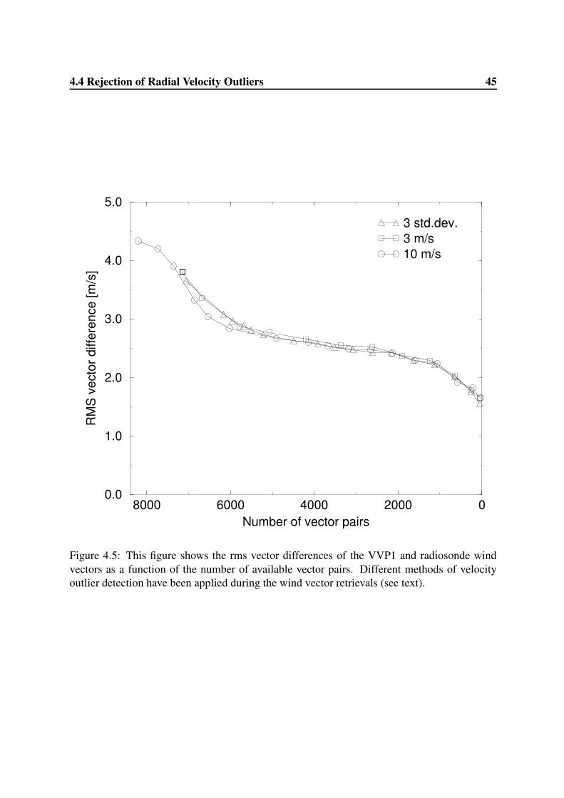
4.4 Rejection of Radial Velocity Outliers 45
02000400060008000Number of vector pairs
0.0
1.0
2.0
3.0
4.0
5.0
RM
S v
ecto
r diff
eren
ce [m
/s]
3 std.dev.3 m/s10 m/s
Figure 4.5: This figure shows the rms vector differences of the VVP1 and radiosonde windvectors as a function of the number of available vector pairs. Different methods of velocityoutlier detection have been applied during the wind vector retrievals (see text).

46 Intercomparison of Wind Profile Retrieval Techniques
radial velocity outliers are removed from the volume scan data to improve the wind vector re-trieval. The velocity outliers are detected by taking the difference of the radial velocity fromthe wind field model using the retrieved parameters and that from the volume scan data. Thethreshold value on this velocity difference can be set in different ways: using a fixed thresholdor using a multiple of the retrieved standard deviation of the radial velocity as a threshold.
In figure 4.5 the rms vector differences of the VVP1 and radiosonde wind vectors is shownas a function of the number of available vector pairs. The threshold for removal of velocityoutliers was determined in different ways: 3 times the standard deviation, a fixed value of3 m/s, and one of 10 m/s. The verification results show that the method for setting the outlierthreshold value is not very critical. The fixed threshold value of 10 m/s gives slightly betterresults than the 3 m/s threshold or the threshold value based on the standard deviation. Thisconfirms the expected non-Gaussian distribution of the errors in the radial velocity data. Themajority of the outliers will be due to isolated dealiasing errors which are characteristic forvelocity data obtained using the dual-PRF technique (Holleman and Beekhuis, 2003). A fixedthreshold value of 10 m/s for the removal of radial velocity outliers in between the two windmodel fits will be applied.

Chapter 5
Performance of VVP Retrieval Technique
5.1 Availability of Wind Profiles
The combination of quality, availability, and error characteristics determines the impact of radarwind profiles for nowcasting or assimilation into NWP models. In the previous chapter a rea-sonable threshold for the radial velocity standard deviation has been selected. The impact ofthis choice on both the availability and the quality of the radar wind profiles will be investigatedin this section and the next two sections, respectively. Using a standard deviation threshold of2.0 m/s histograms of the wind speeds observed by Doppler radar using the VVP1 retrievalmethod have been constructed for three different height ranges. The constructed histogramsfor the 0-2 km, 2-4 km, and 4-6 km height ranges are shown in figure 5.1. The vertical axisrepresents the wind vector count per 1 m/s-wide bin using all available radar wind profiles be-tween 1 October 2001 and 30 June 2002. The vertical bars represent the mean radiosonde windspeeds over the same period. Comparing the histograms for the three height ranges, it is evidentthat the total number of available wind vectors and the mean wind speed are decreasing andincreasing, respectively, with increasing height. The vertical dashed line marks the maximumunambiguous velocity of the Doppler scans using the dual-PRF technique (see section 2.6). Itis remarkable that for the upper height range a signification number of wind vectors with speedsabove the unambiguous velocity are observed. For these high wind speeds the observed VADcurves (see figure 3.1) will be distorted: radial velocities larger than the unambiguous velocitywill be aliased and shifted by 80 m/s. Apparently the wind profile retrieval method is capableof dealing with these velocity outliers.
In table 5.1 the quantitative results of the histogram analysis have been collected. Thetable lists for 1 km height ranges the fraction of the number of available wind vectors to themaximum number of vectors. This “availability fraction” decreases from 0.39 in the lowestheight range to 0.16 in the highest height range. In the boundary layer the radar radiation isscattered by precipitation, refractive-index gradients, insects and birds (Wilson et al., 1994),and above the boundary layer the radiation will be scattered by precipitation only. During

48 Performance of VVP Retrieval Technique
0 10 20 30 40 50wind speed [m/s]
0
1000
2000
3000
4000
5000
6000
Cou
nt
0−2 km2−4 km4−6 km
Figure 5.1: This figure shows histograms of the observed wind speeds for three different heightlayers and using wind speed bins of 1 m/s. The wind speeds are obtained from the radar usingthe VVP1 retrieval method and a standard deviation threshold of 2.0 m/s. The vertical barsrepresent the mean wind speeds as obtained from the radiosonde observations over the sameperiod.
Table 5.1: This table contains the quantitative results of the histogram analysis for 1 km heightranges. For each height range, the total number of available wind vectors (Count), and thefraction number of available vectors to the maximum number (Availability) are listed. Themaximum number of wind vectors is the product of the number of profiles (22610) and thenumber of layers per height range (5).
Height Count Availability0-1 km 44392 0.3931-2 km 46184 0.4092-3 km 34308 0.3033-4 km 28072 0.2484-5 km 24049 0.2135-6 km 18310 0.162

5.2 Quality as a function of Wind Speed 49
the verification period, the synoptical station at De Bilt has reported precipitation in 925 outof 6552 possible cases, i.e., a precipitation occurrence fraction of 0.141. It is evident fromtable 5.1 that the wind vector availability fraction converges to this fraction with increasingheight. The observed availability at low altitudes (0-2 km) is considerably lower than the 0.83and 0.64 at 925 and 850 hPa, respectively, as reported by Andersson (1998). His rms vectordifferences are also considerably higher than the values in figure 4.1, indicating that a differentbalance between availability and quality was chosen.
5.2 Quality as a function of Wind Speed
A reasonable threshold for the radial velocity standard deviation has been selected previously.Using this standard deviation threshold the performance of the wind profile retrieval methodshas been investigated using several quality measures. In this section the performance of theVVP1 retrieval method as a function of the wind speed will be analyzed. For this, the collectedpairs of wind vectors from the VVP1 retrieval and radiosonde with matching time and heightcoordinates have been grouped according to the radiosonde wind speed. As stated previously,radiosondes are typically launched 30 minutes too early and therefore radiosonde profiles ofe.g. 12 UTC are compared with Doppler wind profiles from 11:30 UTC. Quality parameters,like the root-mean square (rms) vector differences, the bias and standard deviation of windspeed and direction, have been calculated for all wind speed groups.
The results of the quality analysis as a function of wind speed (group) are presented infigure 5.2. The upper part of the figure shows the rms vector differences between the VVP1and the radiosonde wind vectors as a function of the radiosonde wind speed. Note that theserms vector differences differ from those in figures 4.1 and 4.2, because the standard deviationthreshold has now been applied to quality control the retrieved wind vectors. When the selectedwind speed is increased from the lowest to the highest group, the rms vector differences isslowly increasing from 2 to 3 m/s. This increase of the rms vector differences is attributedto the increasing horizontal separation between the radiosonde and radar observations withincreasing wind speed.
The middle part of figure 5.2 displays the bias and standard deviation of the wind speedsfrom the VVP1 retrieval with respect to the radiosonde wind speeds. It is evident that thewind speed bias is generally smaller than 0.5 m/s and positive, i.e., the radar wind speeds areslightly higher than those of the radiosonde. The wind speed bias is much smaller than thecorresponding standard deviation, and it is therefore considered to be within acceptable limits.The relatively large positive bias for the lowest wind speed group is most likely due to the re-jection of radial velocities below 2 m/s (see section 3.5). For the highest wind speed group, thebias is −1 m/s which is probably caused by the limited unambiguous radial velocity (40 m/s)of the radar. The required accuracy (standard deviation) of upper air wind speed measurementsis 1 m/s according to the WMO guide on Meteorological Instruments and Methods of Obser-

50 Performance of VVP Retrieval Technique
0
1
2
3
4
5
RM
S v
ec. [
m/s
]
−1
0
1
2
3
Spe
ed [m
/s]
0 10 20 30 40Wind speed [m/s]
0
10
20
30
Dire
ctio
n [d
eg]
Figure 5.2: This figure shows the rms vector differences in the upper frame, the bias (•) andstandard deviation (�) of the wind speed (middle frame), and the bias (•) and standard de-viation (�) of the wind direction (lower frame) as a function of wind speed. These qualityparameters have been obtained from the verification of VVP1 wind vectors against those fromthe radiosonde.

5.3 Quality as a function of Height 51
vation (WMO, 1996). This confirms that the observed wind speed bias is within acceptablelimits, and suggests that the observed standard deviation, which is deduced from a comparisonbetween two measurements, just satisfies the accuracy requirements.
The bias and standard deviation of the wind direction from the VVP1 retrieval with respectto that of the radiosonde are shown in the lower part of figure 5.2. The bias of the winddirection is usually less than 1 degree and thus is negligible. For the standard deviation of thewind direction a strong dependence on the wind speed is observed. This standard deviationdrops from a rather high value of about 35 degrees at low wind speeds to a low value of only3 degrees at high wind speeds. The observed dependence of the standard deviation on the windspeed suggests that the errors in the Cartesian wind field components, the originally retrievedparameters, are (approximately) constant. The wind direction is determined from the ratio ofthe horizontal wind field components and this ratio has a larger error for lower wind speeds.The required accuracy (standard deviation) of upper-air wind direction measurements is 5 and2.5 degrees for wind speeds below and above 15 m/s, respectively (WMO, 1996). The biasof the observed wind direction is within acceptable limits. The observed standard deviationis caused by errors in radar and radiosonde measurements, and by sampling differences. Itappears that for wind speeds above 10 m/s the Doppler radar is capable of providing windprofiles which satisfy the stringent accuracy requirements by WMO.
5.3 Quality as a function of Height
Another and maybe more intuitive way of grouping the wind profile verification data is accord-ing to the height of the retrieved wind vectors. In this section the performance of the VVP1retrieval method and the Rainbow VVP module will be analyzed by verification against ra-diosonde and the Hirlam model. The collected pairs of wind vectors matching in time andheight have been grouped into 1 km thick height layers and several quality measures have beencalculated. The results are presented as profiles in figures 5.3 to 5.7.
Figure 5.3 shows profiles of the bias and standard deviation of the wind speed and directionfor the VVP1 retrieval method. These quality measures have been obtained from verificationagainst radiosonde wind profiles. Because the mean wind speed increases with height (seefigure 5.1), the verification results presented in this figure are strongly correlated to those infigure 5.2 and similar features can indeed be seen. The wind speed bias is slightly positive atall heights and less than 0.5 m/s. The standard deviation of the wind speed is slowly increasingfrom 1.5 m/s at low altitude to about 2.0 m/s at the highest altitude. The same tendencies butmore pronounced are evident from the middle part of figure 5.2. The wind direction bias showsa remarkable sign change between 3 and 4 km altitude. This sign change is not observed in thewind direction bias as a function of wind speed (see lower part of figure 5.2), and it thereforemust originate from a true (unexplained) height effect. The decrease of the standard deviationof the wind direction with increasing height is similar to that with increasing wind speed, but

52 Performance of VVP Retrieval Technique
−2 −1 0 1 2Bias [m/s]
0
1
2
3
4
5
6H
eigh
t [km
]
0 1 2 3 4Std.dev. [m/s]
−5 0 5Bias [deg]
0
1
2
3
4
5
6
Hei
ght [
km]
0 10 20Std.dev. [deg]
Figure 5.3: This figure shows profiles of the bias and standard deviation of the wind speed anddirection as obtained from verification of VVP1 against radiosonde.
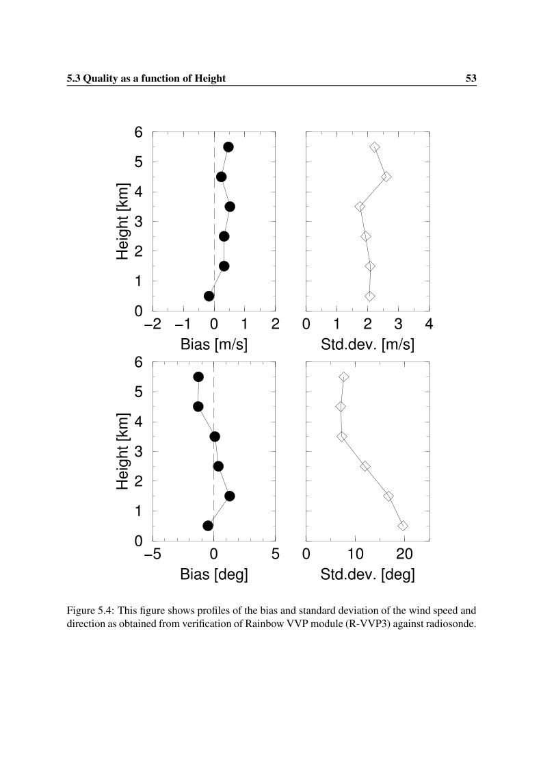
5.3 Quality as a function of Height 53
−2 −1 0 1 2Bias [m/s]
0
1
2
3
4
5
6H
eigh
t [km
]
0 1 2 3 4Std.dev. [m/s]
−5 0 5Bias [deg]
0
1
2
3
4
5
6
Hei
ght [
km]
0 10 20Std.dev. [deg]
Figure 5.4: This figure shows profiles of the bias and standard deviation of the wind speed anddirection as obtained from verification of Rainbow VVP module (R-VVP3) against radiosonde.

54 Performance of VVP Retrieval Technique
−2 −1 0 1 2Bias [m/s]
0
1
2
3
4
5
6H
eigh
t [km
]
0 1 2 3 4Std.dev. [m/s]
−5 0 5Bias [deg]
0
1
2
3
4
5
6
Hei
ght [
km]
0 10 20Std.dev. [deg]
Figure 5.5: This figure shows profiles of the bias and standard deviation of the wind speed anddirection as obtained from verification of VVP1 against Hirlam.

5.3 Quality as a function of Height 55
−2 −1 0 1 2Bias [m/s]
0
1
2
3
4
5
6H
eigh
t [km
]
0 1 2 3 4Std.dev. [m/s]
−5 0 5Bias [deg]
0
1
2
3
4
5
6
Hei
ght [
km]
0 10 20Std.dev. [deg]
Figure 5.6: This figure shows profiles of the bias and standard deviation of the wind speed anddirection as obtained from verification of Rainbow VVP module against Hirlam.

56 Performance of VVP Retrieval Technique
−2 −1 0 1 2Bias [m/s]
0
1
2
3
4
5
6H
eigh
t [km
]
0 1 2 3 4Std.dev. [m/s]
−5 0 5Bias [deg]
0
1
2
3
4
5
6
Hei
ght [
km]
0 10 20Std.dev. [deg]
Figure 5.7: This figure shows profiles of the bias and standard deviation of the wind speedand direction as obtained from verification of Rainbow VVP module at Den Helder againstHirlam.

5.3 Quality as a function of Height 57
it has a smaller amplitude.The bias and standard deviation profiles obtained from the verification of the Rainbow VVP
module against the radiosonde observations are shown in figure 5.4. Comparing the profiles inthis figure with those in the previous figure, the bias profiles of both wind speed and directionmatch very well and the standard deviation profiles are shifted to higher values. In addition, thespeed and directional bias of the R-VVP3 wind vectors are negative below 1 km altitude. Thehigher standard deviations and the remarkable discrepancy between the biases of the VVP1and R-VVP3 wind vectors below 1 km are probably due to the absence of standard deviationthresholding after the final fit and the less stable regression algorithm in the Rainbow VVPmodule.
The retrieved wind profiles have also been verified against profiles from the Hirlam model.Figures 5.5 and 5.6 show the bias and standard deviation profiles from the verification of theVVP1 retrieval method and the Rainbow VVP module, respectively, against the Hirlam model.Comparing these two figures with the corresponding figures from the verification against ra-diosonde, reveals a good qualitative and a fair quantitative match of the bias and standarddeviation profiles obtained with the different verification data. All obvious features of the biasprofiles, like the positive speed bias and the sign change of the directional bias, are reproducedusing the Hirlam data for verification. At low altitudes, the observed speed bias is larger thanfor the verification against radiosonde which is probably due to a negative speed bias in the ini-tialized analyzes of Hirlam. In addition the standard deviation profiles of wind direction matchquantitatively, but those of wind speed are shifted to somewhat higher values. This quanti-tative difference is in correspondence with the larger rms vector differences for verificationagainst the Hirlam model as presented in section 4.3. Thus for De Bilt, verification of windprofiles against the Hirlam model provides the same qualitative insights and almost the samequantitative results as verification against radiosonde.
For the radar in Den Helder, Rainbow VVP wind profiles and corresponding Hirlam profilesare available. Figure 5.7 shows the profiles of bias and standard deviation from the verificationof the R-VVP3 module against Hirlam for the Den Helder radar. At first glance it is strikingthat the profiles only go up to 4 km altitude which is due to the limitation of the scan strategyof the radar in Den Helder (see section 2.6). In the next section the quantitative impact of thislimitation will be investigated further. Other striking features are the large wind speed bias, andvery large standard deviations below 1 km altitude. This is probably due to the inhomogeneousenvironment, the radar is located on land but large water surfaces are nearby in many directions(< 5 km). These land-sea transitions are not fully represented in the Hirlam model due to thelarger grid spacing. In addition these large standard deviations may be caused by interferencefrom sea clutter in the lowest elevation beams.

58 Performance of VVP Retrieval Technique
5.4 Removal of ElevationsUp to now velocity scan data from 10 elevations have been used to retrieve the radar wind pro-files. The elevations are listed in table 2.1. For development of operational scanning strategiesit is important to know whether data from all 10 elevations are really needed to obtain windprofiles of sufficient quality. In addition the radar in Den Helder is currently not allowed to useelevations above 12 degrees. A demonstration of the impact of this limitation on the qualityand availability of the radar wind profiles may provide an impulse to re-open the negotiationswith the naval air base in Den Helder.
The radar wind profiles at De Bilt have been re-calculated from volume scan data using theVVP1 retrieval method and removing data from selected elevations. When the elevations inthe volume scans as listed in table 2.1 are numbered from 0 to 9, the wind profiles have beenre-calculated for the following six scenarios:
Null: Velocity scan data from all elevations are used. This scenario is included for referencepurposes.
Zero: Scan data from elevation “zero” (0.5 degrees) are excluded from the wind profile re-trieval. It is expected that velocity data from this low elevation are contaminated by(sidelobe) clutter and that wind profile retrieval may benefit from this exclusion.
Nine: Scan data from elevation “nine” (25 degrees) are excluded from the wind profile re-trieval. Data from this high elevation may be contaminated by the inhomogeneity of theterminal velocity of the hydrometeors and of (strong) updrafts (see section 3.1).
Even: Velocity scan data from the five even numbered elevations have been excluded from thewind profile retrieval. The impact of the removal of 50% of the scan data on the qualityand availability of the wind profiles can be investigated using this scenario.
Odd: Velocity scan data from the five odd numbered elevations have not been used for thewind profile retrieval. Use is the same to that of the previous scenario.
DenHelder: Scan data from the 3 highest elevations (>12 degrees) have not been used. In thisscenario the “Den Helder limitation” is also applied to De Bilt radar, and the impact ofthis limitation can be investigated.
The availability fractions and rms vector differences with respect to radiosonde wind dataas a function of height are listed in tables 5.2 and 5.3, respectively, for the six scenarios. Theremoval of the lowest elevation from the scan data (scenario zero) improves the quality, i.e.,reduces the rms vector differences, of the retrieved wind vectors below 4 km altitude, but itslightly reduces the availability. This finding supports the idea that the quality of radial velocitydata from the lowest elevation is of poor quality at short ranges due to sidelobe clutter. Theremoval of the highest elevation (scenario nine) has a small effect on the availability, but it

5.4 Removal of Elevations 59
Table 5.2: In this table the wind vector availability fractions are listed as a function of heightfor the six scenarios (see text). A standard deviation threshold of 2.0 m/s has been used toquality control the retrieved wind vectors. The number of wind vectors corresponding to anavailability fraction of 1 is the product of the number of profiles (22610) and the number oflayers per height range (5).
Height Null Zero Nine Even Odd DenHelder0-1 km 0.39 0.36 0.39 0.34 0.37 0.391-2 km 0.41 0.40 0.40 0.38 0.37 0.382-3 km 0.30 0.30 0.29 0.29 0.29 0.243-4 km 0.25 0.24 0.23 0.23 0.24 0.194-5 km 0.21 0.21 0.20 0.20 0.21 0.145-6 km 0.16 0.16 0.15 0.16 0.16 0.04
Table 5.3: In this table the rms vector differences between the VVP1 wind vectors and thoseof the radiosonde are listed as a function of height for the six scenarios (see text). A standarddeviation threshold of 2.0 m/s has been used to quality control the retrieved wind vectors.
Height Null Zero Nine Even Odd DenHelder0-1 km 2.37 2.23 2.37 2.27 2.44 2.371-2 km 2.47 2.40 2.47 2.48 2.61 2.462-3 km 3.02 2.94 2.88 3.02 3.04 2.873-4 km 3.37 3.32 3.23 3.30 3.36 3.244-5 km 3.15 3.16 3.13 3.20 3.12 3.145-6 km 3.10 3.11 3.05 3.13 3.19 3.12
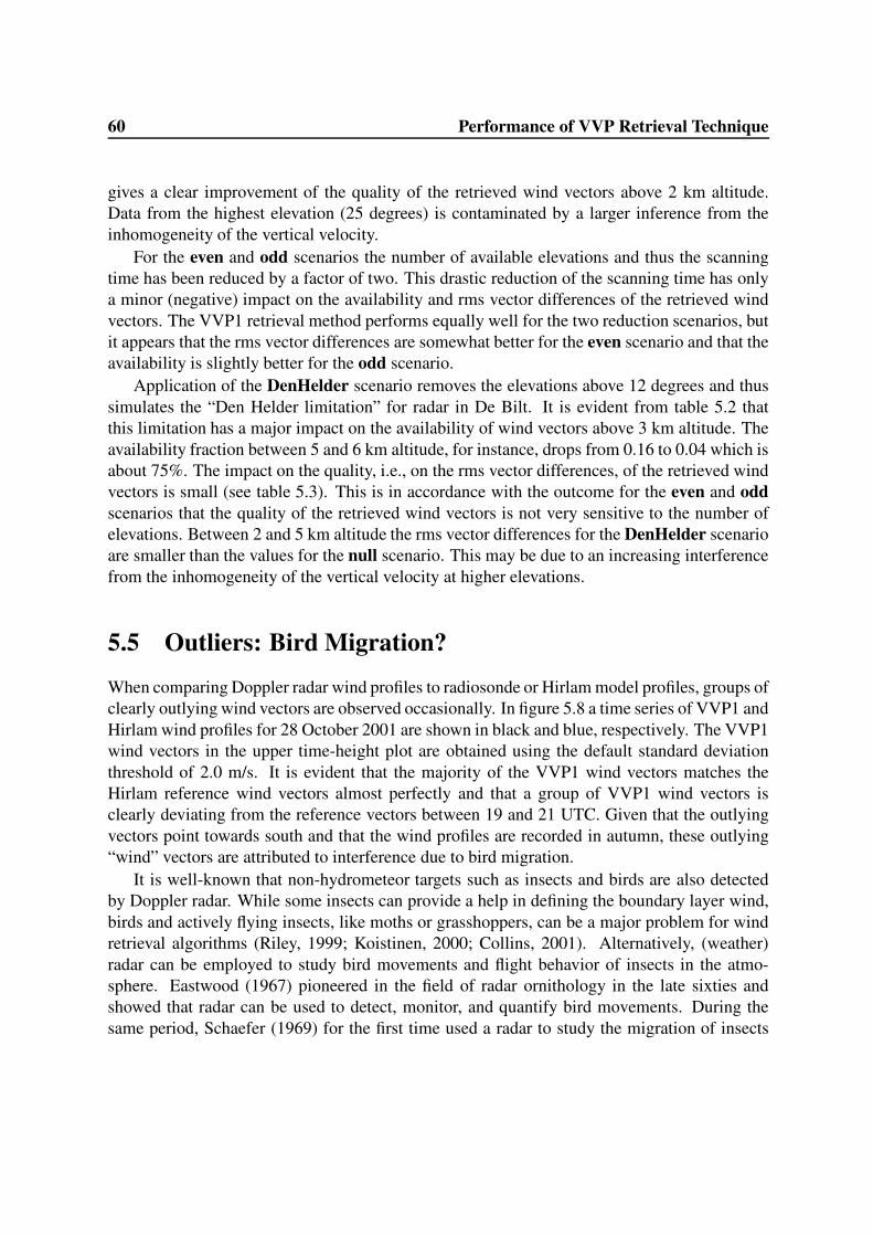
60 Performance of VVP Retrieval Technique
gives a clear improvement of the quality of the retrieved wind vectors above 2 km altitude.Data from the highest elevation (25 degrees) is contaminated by a larger inference from theinhomogeneity of the vertical velocity.
For the even and odd scenarios the number of available elevations and thus the scanningtime has been reduced by a factor of two. This drastic reduction of the scanning time has onlya minor (negative) impact on the availability and rms vector differences of the retrieved windvectors. The VVP1 retrieval method performs equally well for the two reduction scenarios, butit appears that the rms vector differences are somewhat better for the even scenario and that theavailability is slightly better for the odd scenario.
Application of the DenHelder scenario removes the elevations above 12 degrees and thussimulates the “Den Helder limitation” for radar in De Bilt. It is evident from table 5.2 thatthis limitation has a major impact on the availability of wind vectors above 3 km altitude. Theavailability fraction between 5 and 6 km altitude, for instance, drops from 0.16 to 0.04 which isabout 75%. The impact on the quality, i.e., on the rms vector differences, of the retrieved windvectors is small (see table 5.3). This is in accordance with the outcome for the even and oddscenarios that the quality of the retrieved wind vectors is not very sensitive to the number ofelevations. Between 2 and 5 km altitude the rms vector differences for the DenHelder scenarioare smaller than the values for the null scenario. This may be due to an increasing interferencefrom the inhomogeneity of the vertical velocity at higher elevations.
5.5 Outliers: Bird Migration?
When comparing Doppler radar wind profiles to radiosonde or Hirlam model profiles, groups ofclearly outlying wind vectors are observed occasionally. In figure 5.8 a time series of VVP1 andHirlam wind profiles for 28 October 2001 are shown in black and blue, respectively. The VVP1wind vectors in the upper time-height plot are obtained using the default standard deviationthreshold of 2.0 m/s. It is evident that the majority of the VVP1 wind vectors matches theHirlam reference wind vectors almost perfectly and that a group of VVP1 wind vectors isclearly deviating from the reference vectors between 19 and 21 UTC. Given that the outlyingvectors point towards south and that the wind profiles are recorded in autumn, these outlying“wind” vectors are attributed to interference due to bird migration.
It is well-known that non-hydrometeor targets such as insects and birds are also detectedby Doppler radar. While some insects can provide a help in defining the boundary layer wind,birds and actively flying insects, like moths or grasshoppers, can be a major problem for windretrieval algorithms (Riley, 1999; Koistinen, 2000; Collins, 2001). Alternatively, (weather)radar can be employed to study bird movements and flight behavior of insects in the atmo-sphere. Eastwood (1967) pioneered in the field of radar ornithology in the late sixties andshowed that radar can be used to detect, monitor, and quantify bird movements. During thesame period, Schaefer (1969) for the first time used a radar to study the migration of insects

5.5 Outliers: Bird Migration? 61
0 2 4 6 8 10 12 14 16 18 20 22 24
43
21
0
Time [UTC]
Hei
ght [
km]
0 2 4 6 8 10 12 14 16 18 20 22 24
43
21
0
Time [UTC]
Hei
ght [
km]
Figure 5.8: Two time-height plots with the hourly retrieved wind vectors using the VVP1 tech-nique for 28 October 2001. The upper time-height plot is obtained using the default standarddeviation threshold of 2.0 m/s and the lower plot using a threshold of 1.8 m/s. The wind pro-files from the Hirlam model are overlayed in blue. Wind speed and direction are indicated bywind vanes. Each full barb represents a wind speed of 5 m/s and each triangle a wind speed of25 m/s.

62 Performance of VVP Retrieval Technique
in the Sahara. A detailed overview of the relevant properties of bird migration for radar mete-orology is presented by Koistinen (2000). Depending on the species, migrating birds have anair speed between 7 and 20 m/s. The track vector of a migrating bird, which is equal to theoutlying “wind” vector, is the sum of the environmental wind vector (tail wind) and the headingvector of the bird. The heading is usually such that it (partly) compensates the wind drift fromthe final goal. The tail wind plays a crucial role in bird migration, because it determines the in-tensity of the migration and the distribution of the cruising heights. In Northern Europe typicalcruising heights are between 0.5 and 2 km and in the Mediterranean region flight heights up to4 km can be found. Heavy bird migration occurs when the 10 m wind speed is below 8 m/s andthe wind direction is favorable. When the 10 m wind speed is above 11 m/s, the bird is unableto compensate the wind drift and the risk of dangerous wind gusts near the ground increasesrapidly. The other important meteorological factor influencing the intensity of the migration isprecipitation. Heavy precipitation may directly influence the flying capability of a bird, and inaddition it hampers the available navigation senses (Koistinen, 2000).
Using the afore mentioned properties and wind profiles from other sources, a manual di-agnosis of birds migration and/or outlying “wind” vectors is not very difficult. An automaticdetection of bird migration based on radar data only is not straightforward. In the lower frameof figure 5.8 a time-height plot of VVP1 retrieved wind profiles for the same day as the upperframe but with a non-default standard deviation threshold of 1.8 m/s is shown. It is evidentthat application of this slightly more stringent threshold eliminates the outlying “wind” vectorsfrom the profiles in this case. This is in agreement with the observation of Koistinen (2000)that the standard deviation of the radial velocity determined from the wind profile retrieval islarger in bird migration than in rain. The application of a more stringent threshold on the stan-dard deviation is not without a cost. From figure 4.3 it can be deduced that the 10% lowerthreshold leads to a 6% reduction of the number of available VVP1 wind vectors. Wind vectorsfrom clear-air return also have a relatively large standard deviation and these wind vectors willthus be removed primarily. As detailed before the quality and availability of wind profiles arecoupled, and the optimum setting of standard deviation threshold will, therefore, depend on theapplication of the profiles. For nowcasting purposes a high availability of the wind profiles ismost important, while for assimilation in NWP models the quality of the profiles is the mainissue.
An attempt has been made to find a method to eliminate outlying “wind” vectors due tobird migration without reducing the availability of the wind vectors significantly. The proposedmethod is based on the assumed difference in the spatial structure of the radial velocity scandata for precpiptation and migrating birds. During precipitation large continuous areas withvalid radial velocity data are usually present in volume scan data, and in contrast migratingbirds give rise to scattered groups of range bins with valid data. As part of the correctionalgorithm for dual-PRF velocity data a group-size filter has been developed which removesgroups with valid data consisting of less than a minimum number of range bins from the scandata (Holleman and Beekhuis, 2003). This group-size filter has been applied to remove the

5.5 Outliers: Bird Migration? 63
Table 5.4: Elimination of outlying “wind” vectors due to bird migration using group-size filter-ing and reduction of standard deviation threshold. To favor the bird migration “wind”’ vectors,only vectors between 1 and 4 km altitude have been considered. The table lists the appliedstandard deviation threshold (std.dev.), the minimum group-size after filtering (size), the rmsvector differences against Hirlam wind profiles matching within 1.5 hour (rms), the total num-ber of retrieved wind vectors (total), and the number of outlying wind vectors, i.e., vectors withat least 8 m/s offset in the north-south direction with respect to Hirlam (outliers).
Std.dev. Size rms Total Outliers2.0 0 3.6 100456 5412.0 5 3.6 91355 5702.0 10 3.6 87461 5722.0 15 3.6 85407 5692.0 20 3.6 83658 5352.0 25 3.6 82542 5251.8 0 3.5 95632 4181.5 0 3.4 83927 2801.0 0 3.1 47289 87
scattered groups of range bins, assumed to be due to migrating birds, from the volume scanbefore retrieval of the wind profile using the VVP1 technique. Minimum group sizes between5 and 25 range bins have been applied in different runs. It is found that application of thegroup-size filter has a negligible impact on the average quality and availability of the VVP1wind vectors (see table 5.4). The outlying “wind” vectors due to bird migration are recognizedby a large offset of the north-south wind component (8 m/s) with respect to Hirlam profiles(Collins, 2001) and a height between 1 and 4 km. The results of this experiment are listed intable 5.4. Unfortunately, it is evident from the table that application of the group-size filterdoes not reduce the number of outlying vectors. In contrast, the standard deviation thresholdprovides an adequate means to control the number of outlying wind vectors.

64 Performance of VVP Retrieval Technique

Chapter 6
Conclusions and Recommendations
In this scientific report an introduction to Doppler velocity observations and the optimized set-tings of the Doppler radar are presented. In addition, the principles of wind profile retrievalmethods are introduced and different versions of the VAD and VVP wind profile retrieval tech-niques have been described. Finally, an intercomparison of the different implementations of theVAD and VVP retrieval techniques and an extensive verification of VVP wind profiles usingradiosonde and Hirlam profiles have been performed. It is concluded that Doppler radars canprovide good quality wind profiles with a reasonable availability, and operational applicationof the Doppler radar wind profiles is recommended.
The settings of the Doppler radar have been optimized by adjusting the scanning strategyand the parameters of the radar signal processor. The choice for the applied Doppler clutterfilter and the values of threshold qualifiers on the signal processor are based on the outcomeof dedicated experiments. Going through the equations for the wind profile retrieval tech-niques, it is obvious that several stages of simplification can be applied to the VAD and VVPmethods. The intercomparison of these different implementations of the retrieval methods andthe Rainbow VVP module using radiosonde and Hirlam reference profiles revealed that theVVP methods perform better than the VAD methods. In contrast to a VVP retrieval, where allavailable scan data within range is quality controlled at once, all velocity-azimuth circles arequality controlled individually during a VAD retrieval, and this results in a higher rejection rate.Furthermore, it was found that the most simple implementation of the VVP retrieval method,i.e., using only 3 wind field parameters, provides the best horizontal wind data. Due to thenon-orthogonality of the basis functions, addition of higher-order functions with (small) lineardependencies may cause fluctuations of the retrieved parameters. The performance of the Rain-bow VVP module is comparable with the developed VVP implementations. The availabilityand the quality of the wind profiles are coupled as expected, and a threshold on the standarddeviation of the radial velocity as determined by the retrieval method can be applied to shiftbetween high availability and high quality. A standard deviation threshold of 2.0 m/s seems areasonable compromise and has been applied throughout this report.
66 Conclusions and Recommendations
An availability fraction of VVP1 wind vectors of about 0.39 is found in the lowest 1 kmof the troposphere, and at 5-6 km altitude the availability has dropped below 0.16 which isapproaching the fraction of observed precipitation in De Bilt during the verification period(0.14). In the boundary layer the radar radiation is scattered by precipitation, refractive-indexgradients, insects and birds, while above this layer the radiation is scattered by precipitationonly. Verification as a function of wind speed of the VVP1 wind vectors against radiosondedata revealed that the accuracy of the retrieved wind speeds satisfies the WMO requirementsfor upper-air wind measurements and that the accuracy of the retrieved wind directions meetsthe requirements only above wind speeds of 10 m/s. At the cost of availability, application ofa more stringent standard deviation threshold can further improve the accuracy of the retrievedwind vectors. Verification of the VVP1 and Rainbow VVP wind profiles as a function ofheight using radiosonde and Hirlam reference profiles showed that use of Hirlam leads to samequalitative results and slightly different values for bias and standard deviation. The experimentswith selective removal of elevations from volume scan data revealed that the VVP1 retrievalmethod is generally not very sensitive to the loss of elevations, but that the elevation limitationfor the Den Helder radar has a large impact on the availability fraction above 3 km altitude.Bird migration is a potential problem for Doppler radar wind profiles. A method for removalof outlying wind vectors due to bird migration based on the assumed spatial structure of theradial velocity scan data for precipitation and migrating birds has been tested without success,but a lowering of the standard deviation threshold may offer a way out for some applications.
Based on the findings presented in this report, operational application of the Doppler radarwind profiles is highly recommended. Before operational application of the Rainbow VVPmodule for retrieval of wind profiles, a few improvements and extensions should be considered:
1. Implementation of an option to change the number of wind field parameters used by theRainbow VVP module from 3, 6, to 9 parameters and thus increase the complexity of theVVP retrieval.
2. Extension of the retrieval output of the Rainbow VVP module from wind speed anddirection to include the vertical velocity, the number of fitted data points, and the ra-dial velocity standard deviation. Especially the standard deviation can be employed to(further) quality control the retrieved wind vectors (depending on the application, e.g.,assimilation in NWP).
3. Apply of the standard deviation threshold after the second wind model fit instead of afterthe first fit.
4. Change the regression algorithm from the solution using standard normal mode analysisto the more accurate solution by Singular Value Decomposition (SVD). SVD is the curefor round-off errors and for almost singular sets of equations.

Conclusions and Recommendations 67
5. Re-open the negotiations with naval air base in Den Helder on the 12 degree elevationlimitation for the Den Helder radar.
6. Implement a conversion of the wind profiles to BUFR and send the profiles amongstothers to the CWINDE (2003) hub to receive monthly feedback on the availability andquality of the Doppler radar wind profiles.
AcknowledgmentsHans Beekhuis is gratefully acknowledged for his assistance in optimizing the settings of theDoppler radar and for a pleasant cooperation. The guidance and support of Herman Wesselsand Sylvia Barlag are highly appreciated. The punctual reviewing of the manuscript by SanderTijm and Herman Wessels is greatly appreciated.

68 Conclusions and Recommendations

Bibliography
Andersson, T.: 1998, VAD winds from C band Ericsson Doppler Weather Radars. Meteor.Zeitschrift, 7, 309–319.
Boccippio, D. J.: 1995, A Diagnostic Analysis of the VVP Single-Doppler Retrieval Technique.J. Atmos. Ocean. Technol., 12, 230–248.
Browning, K. A. and R. Wexler: 1968, The determination of kinematic properties of a windfield using Doppler radar. J. Appl. Meteor., 7, 105–113.
Caya, D. and I. Zawadzki: 1992, VAD Analysis of Nonlinear Wind Fields. J. Atmos. Ocean.Technol., 9, 575–587.
Cifelli, R., S. A. Rutledge, D. J. Boccippio, and T. Matejka: 1996, Horizontal Divergence andVertical Velocity Retrievals from Doppler Radar and Wind Profiler Observations. J. Atmos.Ocean. Technol., 13, 948–966.
Collins, W. G.: 2001, The Quality Control of Velocity Azimuth Display (VAD) Winds at theNational Centers for Environmental Prediction. 11th Symposium on Meteorological Obser-vations and Instrumentation, AMS, 317–320.
CWINDE: 2003, Website of the Coordinated Windprofiler Network in Europe.http://www.meto.gov.uk/research/interproj/cwinde/.
Dlhopolsky, R. and A. Feijt: 2003, An investigation of the representative heights for atmo-spheric motion vectors. Technical Report TR-249, KNMI.
Doviak, R. J. and D. S. Zrnic: 1993, Doppler Radar and Weather Observations. AcademicPress, second edition, 562 pp.
Eastwood, E.: 1967, Radar Ornithology. Methuen, London, 269 pp.
Foote, G. B. and P. S. DuToit: 1969, Terminal Velocity of Raindrops Aloft. J. Appl. Meteor., 8,249–253.

70 BIBLIOGRAPHY
Gematronik: 2003, Rainbow 3.4 Operator’s Manual. Gematronik GmbH., Raiffeneisenstr. 10,41470 Neuss, Germany.
Gunn, K. L. S. and R. S. Marshall: 1958, The distribution of size of aggregate snowflakes. J.Meteor., 15, 452–466.
Holleman, I. and H. Beekhuis: 2003, Analysis and Correction of Dual-PRF Velocity Data. J.Atmos. Ocean. Technol., 20, 443–453.
Holton, J. R.: 1992, An introduction to dynamic meteorology. Academic Press, third edition.
Klein Baltink, H.: 1998, A long-term intercomparison of windprofiler/RASS and tower mea-surements. Meteor. Zeitschrift, 7, 271–279.
Koistinen, J.: 2000, Bird migration patterns on weather radars. Phys. Chem. Earth (B), 25,1185–1194.
Lhermitte, R. M. and D. Atlas: 1961, Precipitation motion by pulse Doppler radar. 9th confer-ence on Radar Meteorology, AMS, 218–223.
Lindskog, M., H. Jarvinen, and D. B. Michelson: 2002, Development of Doppler radar winddata assimilation for the HIRLAM 3D-Var. HIRLAM Technical Report 52, HIRLAM-5Project.
Marseille, G. and A. Stoffelen: 2003, Simulation of Wind Profiles from a Space-borne DopplerWind Lidar. Q. J. R. Meteorol. Soc., in press.
Matejka, T. and R. C. Srivastava: 1991, An Improved Version of the Extended Velocity-Azimuth Display Analysis of Single-Doppler Radar Data. J. Atmos. Ocean. Technol., 8,453–466.
Matejka, T. J.: 1993, Concurrent Extended Vertical Velocity Azimuth Display (CEVAD). 26thconference on Radar Meteorology, AMS, 463–465.
Meischner, P., C. Collier, A. Illingworth, J. Joss, and W. Randeu: 1997, Advanced WeatherRadar Systems in Europe: The COST 75 Action. Bull. Amer. Meteor. Soc., 78, 1411–1430.
Meulen, J. P. v. d.: 2003, Quarterly reports of the E-AMDAR Quality Evaluation Centre onAMDAR data: 2003-I. EUMETNET report 14, KNMI.
Passarelli Jr., R. E. and A. D. Siggia: 1983, The Autocorrelation Function and Doppler SpectralMoments: Geometric and Asymptotic Interpretations. J. Climate Appl. Meteor., 22, 1776–1787.

BIBLIOGRAPHY 71
Press, W. H., S. A. Teukolsky, W. T. Vetterling, and B. P. Flannery: 1992, Numerical Recipesin C: the Art of Scientific Computing. Cambridge University Press, second edition, 994 pp.
Riley, J. R.: 1999, Radar Returns from Insects: Implications for Meteorological Radars. 29thconference on Radar Meteorology, AMS, 390–393.
Rossa, A. M.: 2000, The COST 717 action: use of radar observations in hydrological and NWPmodels. Phys. Chem. Earth (B), 25, 1221–1224, also: http://www.smhi.se/cost717.
Schaefer, G. W.: 1969, Radar studies of locust, moth, and butterfly migration in the Sahara.Proc. Roy. Ent. Soc. Lond., Series C, 34, 33 & 39–40.
Seltmann, J. E. E.: 2000, Clutter versus radar winds. Phys. Chem. Earth (B), 25, 1173–1178.
Serafin, R. J. and J. W. Wilson: 2000, Operational Weather Radar in the United States: Progressand Opportunity. Bull. Amer. Meteor. Soc., 81, 501–518.
Sigmet: 1998, RVP6 Doppler Signal Processor User’s Manual. Sigmet Inc., 2 Park Drive,Westford, MA 01886 USA.
Sirmans, D., D. Zrnic, and B. Bumgarner: 1976, Extension of Maximum UnambiguousDoppler Velocity by Use of Two Sampling Rates. 17th conference on Radar Meteorology,Seattle, WA, Amer. Meteor. Soc., 23–28.
Srivastava, R. C., A. R. Jameson, and P. H. Hildebrand: 1979, Time-Domain Computation ofMean and Variance of Doppler Spectra. J. Appl. Meteor., 18, 189–194.
Srivastava, R. C., T. J. Matejka, and T. J. Lorello: 1986, Doppler radar study of the trailinganvil region associated with a squall line. J. Atmos. Sci., 43, 356–377.
Tijm, A. B. C. and H. T. Wu: 2000, Assessment of the impact of wind profiler / sodar dataon the mesoscale wind analysis in the Netherlands. Technical report, ASWAN final report,KNMI.
Unden et al., P.: 2002, Hirlam-5 Scientific Documentation. Technical report, Hirlam-5 Project,SMHI, also: http://hirlam.knmi.nl.
Waldteufel, P. and H. Corbin: 1979, On the analysis of single Doppler radar data. J. Appl.Meteor., 18, 532–542.
Wessels, H. R. A. and J. H. Beekhuis: 1997, Stepwise procedure for suppression of anomalousground clutter. COST-75 Seminar on Advanced Radar Systems, EUR 16013 EN, 270–277.

72 BIBLIOGRAPHY
Wilson, J. W., T. M. Weckwerth, J. Vivekanandan, R. M. Wakimoto, and R. W. Russell: 1994,Boundary Layer Clear-Air Radar Echoes: Origin of Echoes and Accuracy of Derived Winds.J. Atmos. Ocean. Technol., 11, 1184–1206.
WMO: 1966, International Meteorological Tables, No. 188, TP. 94. Secretariat WMO, Geneva,Switzerland.
— 1996, Guide to Meteorological Instruments and Methods of Observation, No. 8. SecretariatWMO, Geneva, Switzerland, sixth edition.
Xin, L. and G. W. Reuter: 1998, VVP Technique Applied to an Alberta Storm. J. Atmos. Ocean.Technol., 15, 587–592.