Is there a Retirement-Health Care utilization puzzle ...

Document de travail (Docweb) no 1609

Is there a Retirement-Health Care utilization puzzle?Evidence from SHARE data in Europe

Eve Caroli

Claudio Lucifora

Daria Vigani

Septembre 2016

Is there a Retirement-Health Care utilization puzzle? Evidence from SHAREdata in Europe1

Eve Caroli2, Claudio Lucifora3, Daria Vigani4

Abstract: We investigate the causal impact of retirement on health care utilization. Using SHAREdata (from 2004 to 2013) for 10 European countries, we show that health care utilization increaseswhen individuals retire. This is true both for the number of doctor’s visits and for the intensity ofmedical care use (defined as the probability of going more than 4 times a year to the doctor’s). Thisincrease turns out to be driven by visits to general practitioners’, while specialists’ visits are notaffected. We also find that the impact of retirement on health care utilization is significantly strongerfor workers retiring from jobs characterized by long hours worked - more than 48 hours a week and/orbeing in the 5th quintile of the distribution of hours worked. This suggests that at least part of theincrease in medical care use following retirement is due to the decrease in the opportunity cost of timefaced by individuals when they retire.

Keywords: retirement, health, health care utilization.

Retraite et consommation de soins : Y-a-t-il un mystere ? Une analyse surdonnees europeennes (SHARE)

Abstract : Nous etudions l’effet causal du depart a la retraite sur le recours aux soins medicaux. Nousutilisons l’enquete SHARE conduite dans 10 pays europeens (vagues 2004 a 2013) et nous montronsque le recours aux soins medicaux augmente lorsque les individus prennent leur retraite. Cela vauttant pour le nombre de visites chez le medecin que pour l’intensite du recours aux soins (definiecomme la probabilite d’aller chez le medecin plus de 4 fois par an). Cette augmentation s’avere tireepar les visites chez le generaliste alors que les visites chez le specialiste ne sont pas affectees. Nousmontrons aussi que l’impact du passage a la retraite sur le recours aux soins est significativement plusfort pour les individus dont les heures de travail etaient particulierement longues avant leur depart ala retraite (plus de 48h par semaine ou dans le 5eme quintile de la distribution des heures travaillees).Ce resultat suggere que l’accroissement du recours aux soins suite observe au moment du passage ala retraite est, au moins en partie, du a la reduction du cout d’opportunite du temps a laquelle fontface les nouveaux retraites.

Mots-clefs : retraite, sante, consommation de soins.

1We are grateful to Andrea Bassanini, Agar Brugiavini, Lorenzo Cappellari, Bart Cockx, Eric French, Francis Kra-martz, Muriel Roger and Elisabetta Trevisan for useful comments and suggestions. Previous versions of this paper werepresented at the following Workshops ’Policy Evaluation in Health Care and Labour Markets’ and ’Healthy aging and thelabour market’, both held at UCSC in December 2015, and to the DEMS seminar at Universita di Milano Bicocca, wethank participants for the comments received. All remaining errors are ours. The authors are also grateful to CEPREMAPand to Universita Cattolica (D 3.2 HALM project) for financial support. Daria Vigani gratefully acknowledges hospitalityfrom CREST Insee.

2Universite Paris Dauphine, LEDa-LEGOS, Place du Marechal de Lattre de Tassigny 75775 Paris Cedex 16. e-mail:[email protected]

3Department of Economics and Finance, Universita Cattolica, Largo Gemelli, 1 (20123) Milan. e-mail: [email protected]

4Department of Economics and Finance, Universita Cattolica, Largo Gemelli, 1 (20123) Milan. e-mail:[email protected]

2

1 Introduction

Retirement is a milestone event in the life-cycle of individuals, often associ-

ated with significant changes in lifestyles and behaviors of those involved. The

effects of retirement on a number of health and economic outcomes have been

extensively studied in the literature and, despite the fact that the age of re-

tirement is a fairly predictable event, many studies have reported unexpected

jumps around the age of retirement in the health status of individuals, as well

as in consumption (and savings) patterns. The fact that such jumps are hard

to reconcile with the standard life-cycle theory - under the assumption that

agents are forward looking -, combined with the mixed evidence available from

empirical studies, have fostered a debate as to whether health investments and

consumption (savings) should vary smoothly over the life cycle or, in contrast,

experience discontinuities at the time of retirement.

The standard conceptual framework for analyzing health care utilization

and health investment is the Grossman’s human-capital model (Grossman

1972; 2000). In this model, individuals invest in health for both ‘consump-

tion’ (health provides utility) and ‘production’ motives (healthy individuals

get higher earnings). Within this framework, the stock of health is assumed

to depreciate with age (increasingly in old age) but individuals can increase

their health stock by investing in health inputs (e.g. medical care use, healthy

lifestyles). Health care utilization is expected to increase smoothly with the

aging process, to preserve the health stock, until it becomes too costly doing so:

death occurs when the health stock falls below a given threshold. In this con-

text, both the health stock and investments in health care are optimized over

time and, consistent with the life-cycle theory, no jump should be observed.

In a recent paper, however, Galama et al. (2013) challenge the assumption

that health is always at the ‘optimal’ level and investigate the implications

of corner solutions. They extend the standard Grossman model introducing

retirement as a permanent transition from employment to non-employment.

They show that the ‘optimal’ level of consumption, health investment and

3

health stock can be discontinuous at the age of retirement, as retired individ-

uals reallocate away from health investment toward more consumption goods.

The jump in health investment arise from the fact that health does not influ-

ence income after retirement and from the difference in the marginal utility

of leisure after retirement. The existence of a discontinuous change in health

investment at the time of retirement is what we investigate in this paper.

Early studies on consumption and saving patterns have shown that con-

sumption (savings) significantly decreases (increase) at the time of retirement.

This is known as the “retirement-consumption puzzle” since such changes are

hard to reconcile with the consumption-smoothing pattern predicted by the

standard life-cycle theory when agents are forward looking (Banks et al., 1998;

Battistin et al., 2007).

More recent studies have put forward an explanation for the observed drop

in consumption expenditures after retirement, based on substitution across

categories of goods. In particular, consumption would be shifted from work-

related goods (e.g. clothes, transportation) that are typically bought on the

market, toward time-intensive consumption goods (e.g. recreation, sports,

shopping aiming at finding good deals, cooking) that are home-produced (Aguila

et al., 2011; Hurst, 2008; Miniaci et al., 2010). This change in the composition

of consumption after retirement is likely to be optimal, since retirees have more

leisure time as compared to employed individuals.

This paper investigates whether health care utilization and, in particular,

the number of doctor’s visits change in a discontinuous way at the time of

retirement and whether this “puzzling” jump in health care utilization is as-

sociated with the drop in the opportunity cost of time induced by retirement,

as suggested by the theory. To do so, we use all four waves of the Survey of

Health, Ageing and Retirement in Europe (SHARE) which provides informa-

tion on labor market status, health care utilization (in particular GP’s visits

and visits to specialists) and a wide range of socio-economic and demographic

characteristics (Bolin et al., 2009; Dunlop et al., 2000).

4

Providing causal evidence of the impact of retirement on health care uti-

lization is not straightforward. First, retirement decisions are likely to depend

on individual (observable and unobservable) characteristics and second, health

shocks may also affect the decision of individuals to retire early, further con-

founding the identification of the effects of retirement on medical care use.

We tackle these issues by estimating a fixed-effect IV model. Our identifica-

tion strategy exploits legal retirement ages (i.e. early and ordinary retirement

ages) across European countries to instrument the probability of retirement

(Bonsang et al., 2012; Coe and Zamarro, 2011, 2015).

Our results suggest that health care utilization increases when individuals

retire. This is true both for the number of doctor’s visits and for the intensity

of medical care use (defined as the probability of going more than 4 times

a year to the doctor’s). This increase turns out to be driven by visits to

general practitioners’, while specialists’ visits are not affected. We also find

that the impact of retirement on health care utilization is significantly stronger

for workers retiring from jobs characterized by long hours worked - more than

48 hours a week and/or being in the 5th quintile of the distribution of hours

worked. This suggests that at least part of the increase in medical care use

following retirement is due to the decrease in the opportunity cost of time.

Despite the growing relevance of medical care use for both the understand-

ing of individuals’ behavior, and for the design of suitable fiscal policies aimed

at the 50+ population, only a limited number of studies have addressed the is-

sue of health care utilization after retirement (Boaz and Muller, 1989; Jiménez-

Martín et al., 2004). Their results have been quite mixed so far. Using re-

spectively US and German data, Gorry et al. (2015) and Eibich (2014) hardly

find any significant impact of retirement on health care utilization. Regarding

Europe, Celidoni and Rebba (2015) do not find any effect of retirement on

doctor’s visits. In contrast, Coe and Zamarro (2015) show that the number

of doctor’s visits decreases when individuals transit from employment to re-

tirement, unemployment or inactivity. In this paper, we focus on a sample of

5

EU countries and on retirement rather than other forms of exits from employ-

ment. We improve on the existing literature by providing causal evidence that

medical care use increases when individuals retire, and that at least part of

this increase is due the sharp reduction in the opportunity cost of time taking

place at retirement.

The paper is structured as follows. Section 2 presents our empirical strat-

egy. The data are described in Section 3. Section 4 presents our results and

conclusive remarks are provided in section 5.

2 Empirical strategy

In order to assess the impact of retirement on health care utilization, we specify

the following model:

Vit = γRit +X ′itβ + αi + Tt + uit (1)

where Vit is the number of doctor’s visits of individual i in the 12 months

preceding time t, Rit is a dummy variable equal to 1 if individual i is retired at

time t, X ′it is a vector of demographics, household and job characteristics, αi

is an individual fixed-effect (including country fixed-effects) and Tt are wave

dummies.

A key problem in estimating the impact of retirement on the pattern of

health-care utilization comes from the fact that retirement is also correlated

with individuals’ health stock. The potential changes in health status upon

retirement have been much studied in the literature but the evidence remains

somewhat mixed. As regards physical health, a few studies find a negative ef-

fect of retirement (Behncke, 2012; Dave et al., 2008; Godard, 2016), while oth-

ers find evidence of a substantial improvement following retirement, as leisure

allows more time for health-preserving activities - i.e. sport, healthier lifestyles

- (Celidoni and Rebba, 2015; Coe and Zamarro, 2011; Insler, 2014). As regards

mental health and cognitive functions, they are generally found to be nega-

6

tively affected by retirement (Bonsang et al., 2012; Mazzonna and Peracchi,

2012), although a few studies do not find any significant impact (Eibich, 2014;

Lindeboom and Kerkhofs, 2009; Thompson and Streib, 1958). Overall, it is

not clear whether one should expect an increase or a decrease in health status

at the time of retirement (Bassanini and Caroli, 2015). In order to take into

account the potential impact of retirement on health, we introduce a vector of

health controls, H ′it, in our regression:

Vit = γRit +X ′itβ1 +H ′itβ2 + αi + Tt + uit (2)

The number of visits an individual pays to the doctor is also likely to

depend on several unobservable characteristics (e.g. individual time preference,

latent health status etc.), that may also impact her retirement decision Rit. As

long as individual unobservable heterogeneity is time-invariant, the inclusion of

individual fixed effects in the regression, αi, delivers consistent estimates of γ.

This condition, however, is unlikely to hold in general. Time-varying omitted

characteristics, such as own or partner’s negative health shocks, are indeed

likely to affect both the number of doctor’s visits and retirement decisions.

They may even generate some reverse causality if the doctor recommends that,

given her health conditions, the individual should stop working.

To tackle these problems, we also estimate a FE-IV (Fixed-Effects Instru-

mental Variable) model. Our identification strategy exploits the fact that, as

individuals reach legal retirement age, the financial incentive they have to retire

strongly increases. This allows us to estimate the causal impact of retirement

on health care utilization.

In most European countries, retirement occurs either at the Ordinary Re-

tirement Age (ORA) - that is the age at which workers are eligible for full

old-age pensions - or at an Early Retirement Age (ERA) - which represents

the earliest age at which retirement benefits can be claimed conditional on a

given number of years of social security contributions. This is evidenced in

Appendix Figures A1 and A2 that display the shares of retirees and newly

7

retired workers as well as the ‘Early’ and/or ‘Ordinary’ retirement-age thresh-

olds (computed as averages over the period), by age, for each gender and

country. The age-retirement profiles appear quite different across gender and

countries. In many countries the early-retirement-age threshold is lower for

females, as compared to males, which means that on average - conditional on

social security contributions - females are eligible for retirement at an earlier

age. In general, the trend in the share of newly retired workers reveals an

increase in the probability of retirement as individuals approach the Early-

Retirement-age threshold (particularly in Austria, Belgium, France and Italy),

while trends tend to diverge from that point until the Ordinary Retirement

Age: the share of newly retired workers further increases in some countries (i.e.

Germany, The Netherlands, Spain, Switzerland, Denmark) while it declines in

others (i.e. Belgium, France and Austria). In other words, depending on the

interaction between the retirement rules in each country and the structure

of financial incentives, the ‘Early’ and ‘Ordinary’ retirement-age thresholds

account for most of the changes in individuals’ probability of retirement.

In practice, we take advantage of the variability of both ERA and ORA

across countries and use 2 instrumental variables, Yict and Zict, respectively

defined as dummy variables equal to 1 if the individual is above the gender-

specific Early - resp. Ordinary - retirement-age threshold in country c in year

t.2

Yict = 1 if ageict > ERAc,t

Zict = 1 if ageict > ORAc,t

Note that identification here does not rely on the change in early or ordinary

retirement ages across cohorts, but on the increase in the individual probability

of retiring as individuals become eligible for pension benefits in their country

of residence. In other words, the discontinuity in eligibility rules generates an2See table A1 in the Appendix.

8

exogenous shock to retirement decisions which is what we use to instrument

individual retirement status.

One problem with our data is the lack of information on the actual num-

ber of years of social security contributions. Hence, in countries where the

ERA threshold is particularly low (Italy for example), and for those groups of

workers with incomplete career spells (e.g. due to non-participation or long

unemployment spells), the conditionality of a minimum number of years of

contributions is likely to be binding and the ERA cutoff is unlikely to be a

good predictor of the probability of being retired. In this case, the ORA cutoff

is likely to do a better job in instrumenting retirement decision.

Note that, given the panel structure of our data, our identification relies on

individuals who retire across waves. This approach identifies the local average

treatment effect (LATE) - i.e. the effect of retirement on the subpopulation

whom the instrument has induced to retire. So, the point estimate on the

retirement variable, γ, in the FE-IV model, has to be interpreted as the local

average short-term effect of retirement on health care utilization.

3 Data and descriptive statistics

3.1 Data and sample selection

We use data from the Survey of Health, Ageing and Retirement in Europe

(SHARE). This is a multidisciplinary and cross-national survey collecting in-

formation on individuals’ health, socio-economic status, household’s income

and wealth, as well as family networks. More than 85,000 individuals, aged

50 or older - and their partners - from 20 European countries have been inter-

viewed. Five waves of data, from 2004 to 2013, are currently available (one of

which is a retrospective survey). We use the 2004, 2006, 2011 and 2013 waves

keeping only countries that were present in all waves.3

Our sample includes individuals that we observe for at least two consecutive3Austria, Belgium, Germany, Sweden, Spain, Italy, France, Denmark, Switzerland and

the Netherlands.

9

waves, aged 50 to 69 and who are either employed or retired in each wave.4 We

further restrict our sample excluding individuals permanently living in nursing

homes and those who retired because of own ill health. After dropping all

individuals with missing values on the variables of interest, our final sample

consists of 2,883 individuals (9,266 observations).5

3.2 Variables

Health care utilization

Our measure of health care utilization is drawn from a question asking the

respondent how many times she has seen a doctor over the past 12 months.6 A

breakdown of the total number of doctor’s visits between general practitioner’s

and specialist’s visits is also available up to 2011.

We also construct a measure of “high intensity” in the use of physician services,

as a binary indicator which takes value one when the number of doctor’s visits

is larger than the median value for retirees (i.e. more than 4 visits in the past

12 months).

Retirement

The definition of retirement we adopt in our analysis follows that com-

monly used in the literature (Mazzonna and Peracchi, 2012; Rohwedder and

Willis, 2010), where an individual is considered to be retired when leaving the

labor force permanently (i.e. retirement is an absorbing state). In practice,

retirement is coded using respondents’ self-reported employment status in each

wave. Note that SHARE also provides information about the exact year and

month the individual left the labor market, which we use in some robustness4So, our sample contains individuals who were employed all years, retired all years or

who retired between waves. Retirement is therefore an absorbing state.5Among our 2,883 individuals, about 51% are observed in all 4 waves, 19% in 3 consec-

utive waves and 30% are present in only two consecutive waves.6The exact wording is: “About how many times in total have you seen or talked to a

medical doctor about your health (last 12 months)?”. Dentist’s visits and hospital staysare excluded, but emergency room or outpatient clinic visits are included. We consider asoutliers, and therefore exclude, individuals reporting a number of visits higher than threetimes the standard deviation.

10

checks.7

Our definition of retirement departs from that of Coe and Zamarro (2015)

who consider as retired all individuals who report to be either retired or home-

makers or sick and disabled or separated from the labor force or unemployed.

The argument they give in favor of such a comprehensive definition of retire-

ment is that individuals often report to have retired when they have left their

“career” job even if they are still working part-time or full-time. However, this

does not seem to be a major problem in the SHARE data since self-assessed re-

tirement appears to be strongly correlated with the retirement status retrieved

from the year/month-of-retirement variable - with a coefficient of correlation as

high as 0.96 - as well as consistent with ordinary and early retirement eligibility

ages in the country of residence. Given that our identification strategy relies

on the exogenous shock to retirement decisions generated by the discontinuity

in pension eligibility rules at ERA and ORA, we adopt a restricted definition

of retirement that only includes individuals who report to have retired from

work. We exclude individuals who have left employment for unemployment

or inactivity since, in our identification strategy, they are likely to be non-

compliers.8 This should make our instrument stronger if anything. However,

to account for possible biases in self-reported retirement, we run a robustness

test where we exclude from the sample individuals who report to be retired

but did nevertheless some paid work in the previous two weeks.

Control variables

In our empirical analysis we include a large set of controls, capturing indi-

vidual, household and job characteristics. Demographic controls include age

(continuous), education (primary/lower-secondary, upper/post-secondary and7Since the retirement date (the exact year and month) as reported by the respondent is

likely to be affected by measurement error (due to ‘recall bias’), in the main analysis wechoose to rely on the self-reported employment status. We use the information on the date ofretirement only after performing some cleaning and consistency checks, and we then retrievea binary retirement variable that takes value one if the distance between the year/month ofinterview and the year/month of retirement is non-negative.

8As a consequence, as mentioned in Section 3.1 above, our sample only contains individ-uals who are either employed or retired since, for most of those who are either unemployedor inactive there is probably little change in the opportunity cost of time upon retirement.

11

tertiary), a binary indicator for living with a spouse or partner, household size

and a dummy variable for having children. Job characteristics are captured

by industry (1-digit NACE classification) and occupational dummies (1-digit

ISCO-88 classification).

Among the other personal characteristics of the sampled individuals that we

control for, we include household income and ability to make ends meet. House-

hold income is recoded into deciles and includes annual income from employ-

ment, self-employment or pension, as well as regular payments received by

any member of the household. We also use a subjective measure of household

financial distress drawn from a question that asks individuals: “Thinking of

your household’s total monthly income, would you say that your household is

able to make ends meet [with great difficulty ... easily]”, and recode it into a

dummy variable taking value 1 if they make ends meet with difficulty or great

difficulty and 0 otherwise.

Finally, since health status has been found to be a relevant predictor of health

care utilization in the literature, we condition on individuals’ health in our

analysis (Bolin et al., 2009; Redondo-Sendino et al., 2006; Solé-Auró et al.,

2012).9 We include in our regressions a set of controls for self-assessed health,

diagnosed conditions and an indicator of mental health. Self-assessed health is

captured with a binary indicator taking value 1 if the individual reports to be

in poor or fair health, based on a 5-point scale variable (ranging from “poor” to

“excellent”).10 In order to get a more objective measure of individuals’ health

status, we build a summary indicator defined as the sum of all medical con-

ditions that have ever been diagnosed by a doctor,11 and an index of mental9While we account for time-invariant unobserved heterogeneity in health conditions across

individuals, we cannot rule out that health controls might be endogenous in our model.Hence, to check the robustness of our results, we also estimate the FE-IV specificationwithout health controls.

10In the first wave of SHARE (2004), half of the sample was randomly assigned to a 5-pointscale for self-reported health status defined as: “excellent”, “very good”, “good”, “fair” and“poor”. The other half was assigned to a 5-point scale defined as: “very good”, “good”, “fair”,“bad” and “very bad”. Looking at the distributions across categories for the two subsamples,we include in the binary indicator of poor health status those individuals that have answered“fair” and “poor” on the one hand, and “very bad”, “bad” and “fair” on the other hand.

11These conditions include: heart attack, high blood pressure or hypertension, high choles-terol, stroke, diabetes, chronic lung disease, arthritis, cancer, stomach or duodenal ulcer,Parkinson disease, cataracts and hip or femoral fractures.

12

health (EURO-D depression scale ranging from 0 to 12, where higher values

mean more depressed).

3.3 Descriptive statistics

Table 1 reports summary statistics for respondents’ demographic characteris-

tics, health status and doctor’s visits, for the whole sample and separately for

employed and retired individuals (pooling the four waves over 2004-2013).

The upper panel of Table 1 shows that there are no relevant differences

between employees and retirees as regards demographic characteristics: the

size of the household, the probability of having at least one child and the

share of individuals living with a spouse or partner appear to be homogeneous

across both groups, while retirees are on average older (64 versus 58 years-

old) and have a lower level of education. Conversely, the lower panel of the

table presents significant differences in terms of health status and health care

utilization. The share of individuals reporting to be in poor health is 20%

among retirees, as compared to only 12% among employed individuals. Using

a more objective measure of health status, we see that, on average, retirees

present more than one diagnosed chronic condition (1.22), as compared to 0.80

only for the sample of employed individuals.

Retirees show a greater use of medical care, with an average of 4.5 visits

over the past 12 months (as compared to 3.2 for employed individuals) and a

median of 4 (as compared to 2 for employed individuals). 38% of them went

to see a doctor at least 5 times in the past year (as compared to only 24% of

employed individuals).12

The fact that retirees have a more intensive use of physician services than

employed individuals is observed at all ages. As shown on the left-hand-side

panel of Figure 1, the number of visits does not vary much with age, but it is

significantly lower for employees as compared to retirees (particularly from age

59 onward). The sharp drop for employees aged 67 and over is likely to reflect12Description and means of all other control variables can be found in Table A2 in the

Appendix.

13

a selection effect: only individuals with better-than-average health are still in

employment at older ages. A similar pattern is observed for the intensity of

medical care use (see right hand side panel of Figure 1).

4 Results

4.1 Retirement and health care utilization

We first estimate the impact of retirement on health care utilization by pooled

OLS and then with individual FE. The main results are reported in Tables 2

and 3 respectively. We consider different specifications of our baseline model.

First we only include demographic controls along with wave and country fixed

effects (columns 1 and 4). Second, we add to the previous specification a set of

industry and occupational dummies as well as income decile dummies (columns

2 and 5). Finally, we also control for the health status of individuals (columns

3 and 6). As dependent variables we consider both the number of doctor’s

visits (columns 1 to 3) as well as our ‘high intensity’ health care utilization

indicator (columns 4 to 6).

The number of doctor’s visits and the probability of intensive use of medical

14

care both increase with age and are found to be higher for females as compared

to males (columns 1-2 and 4-5 in Table 2). In line with previous findings

in the literature, health care utilization increases as the individual’s health

status deteriorates, being higher for individuals who report poor self-assessed

health, a larger number of diagnosed conditions and a higher depression index

(columns 3 and 6). Interestingly, the effect of age on the number of visits and

on the probability of paying more than 4 visits a year becomes insignificant

once controlling for health indicators, thus suggesting that the reason why older

people visit the doctor more often is because their overall health is poorer. This

is not the case for gender: its effect remains significant even after conditioning

on health controls, suggesting that women are more concerned about their

health than men are.

Coming to the the relationship between retirement and the number of doc-

tor’s visits, we find a positive and statistically significant coefficient suggesting

that retirees go more often to the doctor’s as compared to employed individu-

als (columns 1 and 4 of Table 2). The retirement gap in the number of visits

is around 0.6 per year, which represents a 20% difference computed at the me-

dian of the sample. Retired individuals also show a higher intensity of medical

care utilization, as their probability to see the doctor more than 4 times a

year is about 6% higher than for individuals who are in employment. These

differences are, if anything, larger when income, occupation and industry dum-

mies are also taken into account (columns 2 and 5). When individual health

is controlled for, the gap in the number of visits between retirees and em-

ployed individuals goes down to 14%, suggesting that part of the effect found

in columns (1)-(2) and (4)-(5) was due to the fact that unhealthy individuals

both tend to retire earlier and to go more often to the doctor’s.

The estimated retirement gap is somewhat smaller when time-invariant

unobserved characteristics are controlled for (Table 3): retirement induces a

9% increase in the number of doctor’s visits and a 4% higher probability of

‘high intensity’ in health care utilization. As before, this may be due to the

15

fact that poor health - along unobserved dimensions - is correlated both with

the probability of retiring and with health care utilization. However, it should

be stressed that if the retirement status is measured with error, the estimated

effect is likely to suffer from attenuation bias, and particularly so when a FE

estimator is used. Despite such downward bias, our results do suggest that

doctor’s visits tend to increase when individuals retire.

In the upper panel of Table 4, we report the estimates of the two-stage least

square within estimator (FE-IV), while first-stage estimates are presented in

the lower panel. In the first stage we estimate the probability of retiring

between waves by means of a linear fixed-effect probability model.

The results reported in columns (1) and (4) correspond to a specification

that uses minimum statutory ages for early retirement (i.e. ERA) as the only

instrument. Alternatively, columns (2) and (5) use the age threshold at which

individuals become eligible for ordinary pension benefits (i.e. ORA) as the

sole instrument. Eventually, in columns (3) and (6) both ORA and ERA are

used to instrument individuals’ retirement decisions. In each specification, the

instruments show a sizable and statistically significant effect on the probabil-

ity of retiring. When both instruments are included, the effect of ERA on

retirement appears to be larger than that of ORA. The F-stat for the joint

significance of the instruments shows that both variables are significant pre-

dictors of the probability of retiring and the overidentification test supports

the validity of the exclusion restrictions.

Estimates of the effect of retirement on the number of doctor’s visits in

the upper panel of Table 4 display statistically significant coefficients when

ORA or both ERA and ORA are used as instruments. In contrast, results are

only marginally significant when using ERA alone. Whatever the instrument

we use, the point estimates in the second-stage are much larger than when

estimated by OLS or FE. They turn out to be slightly larger when instrument-

ing retirement decisions with ORA than with both ORA and ERA and they

are smallest when using ERA alone. In all cases, however, they suggest that

16

moving from being employed to retirement causes an increase in the number

of doctor’s visits and in the probability of intensive use of physician services

(i.e. more than 4 visits a year).

The reason why we find different results when using either ERA alone,

ORA alone or both instruments together is likely to be due to differences in

the groups of compliers. As previously discussed, our FE-IV estimates retrieve

a Local Average Treatment Effect, that is the effect of retirement on those

who effectively retire at the corresponding age threshold (Angrist and Pischke,

2009). When using only ORA to instrument retirement decisions, we capture

the effect on those individuals who retire at a later age and would not have

done so earlier. By contrast, when we use both ERA and ORA, we are more

likely to get an average effect on all those individuals who have retired between

the earliest and the latest age thresholds. In other words, we may expect that

using both instruments allows to account for the effect of retirement on a

larger and more heterogeneous pool of individuals. The latter includes those

who have been reducing their working time before retirement, those who have

been laid-off and offered an early exit and, last but not least, all the selected

groups who, for various reasons, have been granted generous early retirement

schemes. For most of those individuals, the effect of retiring on the number of

doctor’s visits is likely to be negligible as compared to full-time workers and

to employees who used to work long hours, and experience a sharp change in

the work-leisure trade-off after retirement.

To explore whether the reduction in the opportunity cost of time generated

by retirement is actually a driving factor of the increase in health care utiliza-

tion, we investigate whether the effect of retirement varies for those individuals

retiring from a job characterized by long hours worked. In Table 5, we interact

our retirement variable with a working-time dummy taking value 1 when the

number of hours worked by the individual in his last job before retirement was

above 48 hours a week13 (columns 1 and 3) or alternatively, with a binary indi-1348 hours is the maximum average weekly working time set by the 2003 EU Working

Time Directive.

17

cator for being in the upper quintile of the distribution of weekly hours worked

(columns 2 and 4). By doing so, we again retrieve a LATE estimate of the

heterogeneous impact of retirement on health care utilization for individuals

who are likely to experience a sharp decrease in the opportunity cost of time

upon retirement.

Whatever the indicator we use, our results suggest that the increase in the

number of doctor’s visits at the time of retirement is largest for individuals who

used to work long hours before retiring: the point estimates on the interaction

between retirement and each of the two dummy variables for long hours are

indeed positive and significant at the 5% level. Similar results are found when

considering the probability of going to the doctor’s more than 4 times a year:

the impact of retirement turns out to be stronger for individuals who used to

work more than 48 hours a week and for those in the upper quintile of the

distribution of hours worked. This suggests that the increase in health care

utilization observed at the time of retirement is at least partly explained by

the reduction in the opportunity cost of time.

One could be concerned however that the differential impact of retirement

on health care utilization estimated in Table 5 could capture gender-specific

behaviors to the extent that men tend to work longer hours than women. To

control for this potentially confounding factor, we re-estimate the specification

used in Table 5 also interacting retirement with gender. As shown in Table

6, the increase in the number of doctor’s visits at the time of retirement - as

well as, in the probability of high intensity’ health care utilization - is mostly

driven by male behavior while the estimated effect for females is essentially

zero. Notice, however, that despite this differential effect by gender, the re-

tirement gap in doctor’s visits remains stronger for those individuals who used

to work long hours before retiring: the point estimates on the interactions of

retirement with the dummy variables for working more than 48 weekly hours

and being in the upper quintile of the distribution of hours worked are still

positive and statistically significant at least at the 10% level.

18

In Table 7, we estimate our model separately for the number of visits paid

to a general practitioner and to a specialist. Our results suggest that the strong

increase in the number of doctor’s visits reported in Tables 5 and 6 for those

individuals retiring from long-hour jobs - either more than 48 hours or in the

upper quintile of the distribution of hours worked - is essentially driven by

visits to the GP’s (columns 2 and 3), whereas the impact is not statistically

significant for specialists (columns 5 and 6). As can be seen when considering

columns (1)-(3) and (4)-(6), poor self-rated health and a higher number of

diagnosed conditions raise the number of visits to both types of doctors. In

contrast, depression has a positive effect, but only on visits to the general

practitioner’s (GP) while it does not seem to affect specialists’ visits.

4.2 Robustness checks

In order to test the robustness of our main findings, in this section we perform

a number of sensitivity checks, experimenting with different specifications and

samples, altering the definition of the retirement variables as well as estimating

a dynamic specification.

One could be concerned that health controls could be endogenous if e.g.

individuals who invest in preventive care both tend to go more to the doctor’s

and end up being in better health than others. This would generate a bias

when estimating our FE-IV model to the extent that we cannot instrument the

health status because of the lack of proper instrumental variables. To tackle

this issue, we estimate a FE-IV specification without health controls - i.e. with

a second stage corresponding to equation (1). As shown in Table A3 in the

Appendix, the results are virtually unchanged. The same holds for all our

key results: when re-estimating the models corresponding to Tables 5, 6 and

7 without health controls, the point estimates and standard errors are almost

identical.14 This suggests that endogeneity of health variables is not a major14Results available upon request

19

issue in our main results.

In the analyses conducted so far, retirement has been defined on the basis

of the employment status reported by individuals. One problem with this

definition is that individuals may report to be retired even though they are still

working. To account for this, we replicate our analysis using two alternative

definitions of retirement. First, exploiting the available information on the

declared year and month of retirement, we construct an indicator of retirement

status where individuals are considered to be retired if the difference between

the year/month of interview and the year/month of retirement is non-negative.

Second, relying on self-reported retirement status, we exclude from the group

of “retired” all individuals who performed any paid work during the two weeks

preceding the interview.

Table A4 in the Appendix shows the results of these exercises. When re-

running our FE-IV estimates using an indicator of retirement computed on

the basis of the year/month in which individuals retired (Panel A), we find

very similar results to those obtained in Tables 4 and 5. When instrumenting

retirement status with both ORA and ERA, the number of doctor’s visits and

the intensity of medical care use turn out to increase significantly at the time

of retirement (columns 1 and 4). This increase also appears to be significantly

stronger for individuals retiring from long-hour jobs - whatever the measure

we use for long hours (columns 2-3 and 5-6).

When we restrict the definition of retirement to individuals who report to be

retired and have not performed any work in the two preceding weeks (Panel

B), the effect of retirement on medical care use turns out to be even stronger.

However, for retirees who used to work long hours before retiring, the increase

in leisure time associated to retirement only affects the probability of high-

intensity of health care utilization (i.e. more than 4 doctor’s visits in the

preceding 12 months). As regards the number of doctor’s visits, it is positively

impacted by retirement but not more so for retirees who used to work long

hours.

20

Given the cross-country dimension of our data, one additional concern could

be that our results are driven by a particularly large effect of retirement on

health-care utilization in a specific country. However, when re-estimating our

model excluding one country at a time, results are virtually unchanged - see

Appendix Table A5 - Line 1.

Since a number of unobservable country-specific characteristics may change

over time, we also augment our FE-IV specification including country-specific

time trends (i.e. wave*country interaction terms) and find very similar results

(see Appendix Table A5 - Line 2). Finally, results are also virtually unchanged

if we introduce country-specific age instead of time trends (see Appendix Table

A5 - Line 3).

We also investigate the dynamic properties of health care utilization. Fol-

lowing Coe and Lindeboom (2008) and Godard (2016), we estimate a simple

dynamic IV version of our model by 2SLS, on the restricted sample of indi-

viduals who were employed at baseline interview.15 We find that the lagged

number of visits is a significant predictor of doctor’s visits in the next period

(i.e. in wave t + 1) and that the effect of retirement is still positive and sta-

tistically significant (at the 10% level) on both the number of visits and the

probability of intensive health care utilization (see Appendix Table A6).16

5 Conclusions

In this paper, we have established that health care utilization increases at

the time of retirement: both the number of doctor’s visits and the probabil-

ity of intensive health care utilization increase when individuals move from

employment to retirement. We argue that this increase can be explained by15We specify the dynamic model as follows:

Vi,t+1 = δVit + γRi,[t,t+1] +X ′itβ1 +H ′itβ2 + Tt + εit

whereVi,t+1 is the number of doctor’s visits in wave t+1, Vit is the number of doctor’s visitsin wave t and Ri,[t,t+1] is a dummy variable taking value 1 if the individual retired betweenwaves t and t+ 1.

16We instrument retirement with a binary indicator taking value 1 when individuals reachthe ERA/ORA thresholds between waves t and t + 1. All the other controls are the sameas reported in Table 4.

21

the sharp drop in the opportunity cost of time that retirees experience upon

retirement. The latter is likely to change their consumption pattern away

from work-related goods and in favor of more time-intensive activities, such

as medical care use. Consistent with these hypotheses, we find that the effect

of retirement on health care utilization is significantly larger for individuals

retiring from jobs characterized by long hours worked. We also find that the

increase in health care utilization at the time of retirement is essentially due to

men rather than women’s behavior and that it is driven by visits to the GP’s

while specialists’ visits are not significantly affected.

One interpretation of the above findings is that the optimal amount of

health care utilization increases, at the time of retirement, due to the implicit

decrease in the cost of time inputs. However we cannot exclude that alternative

mechanisms be at work. For example, it may well be the case that, when

still employed, individuals are rationed in terms of leisure time allocation and

thus unable to reach their optimal choice of health care utilization. Moreover,

consistent with our results, this effect is expected to be stronger for individuals

working long hours before retiring.

While our identification strategy does not allow us to distinguish between

these alternative hypotheses, it is clear that their implications differ substan-

tially. In the first case, conditional on health status, the number of visits to

the GP is likely to be optimal both before and after retirement. Conversely, in

the second case, the number of times individuals visit their GP is suboptimal

before retirement and jumps towards the optimal level only after they retire.

The implications for health policy also differ substantially under the two al-

ternative hypotheses. If the increase in the number of visits after retirement is

the result of individuals‘ short-run response to a sudden change in the oppor-

tunity cost of leisure time there seems to be little scope for policy intervention.

Conversely, if the increase in health care utilization upon retirement reflects

a jump to the optimal level of health care for previously time-rationed indi-

viduals, concerns for public-health may arise. For example, it may imply that

22

senior workers do not get enough health care towards the end of their career,

which may further generate health problems particularly in a context in which

the official retirement age has been raised. Of course, at this stage, whether

the level of health care utilization of older workers is optimal or not remains

an open issue.

23

References

Aguila, E., Attanasio, O. and Meghir, C. (2011), ‘Changes in consumption at

retirement: evidence from panel data’, Review of Economics and Statistics

93(3), 1094–1099.

Angrist, J. and Pischke, J.-S. (2009), Mostly Harmless Econometrics: An Em-

piricist’s Companion, Princeton University Press.

Banks, J., Blundell, R. and Tanner, S. (1998), ‘Is there a retirement-savings

puzzle?’, American Economic Review 88(4), 769–788.

Bassanini, A. and Caroli, E. (2015), ‘Is work bad for health? The role of

constraint vs choice’, Annals of Economics and Statistics (119-120), 13–37.

Battistin, E., Brugiavini, A., Rettore, E. and Weber, G. (2007), ‘The re-

tirement consumption puzzle: evidence from a regression discontinuity ap-

proach’, University Ca’Foscari of Venice, Dept. of Economics Research Pa-

per Series (27/07).

Behncke, S. (2012), ‘Does retirement trigger ill health?’, Health Economics

21(3), 282–300.

Boaz, R. F. and Muller, C. F. (1989), ‘Does having more time after retirement

change the demand for physician services?’, Medical Care pp. 1–15.

Bolin, K., Lindgren, A., Lindgren, B. and Lundborg, P. (2009), ‘Utilisation of

physician services in the 50+ population: the relative importance of indi-

vidual versus institutional factors in 10 European countries’, International

journal of health care finance and economics 9(1), 83–112.

Bonsang, E., Adam, S. and Perelman, S. (2012), ‘Does retirement affect cog-

nitive functioning?’, Journal of Health Economics 31(3), 490–501.

Celidoni, M. and Rebba, V. (2015), ‘Healthier lifestyles after retirement in

Europe? Evidence from SHARE’, "Marco Fanno" Working PapersWP(No.

0201).

24

Coe, N. B. and Lindeboom, M. (2008), ‘Does retirement kill you? Evidence

from early retirement windows’, IZA Discussion Paper DP(No. 3817).

Coe, N. B. and Zamarro, G. (2011), ‘Retirement effects on health in Europe’,

Journal of Health Economics 30(1), 77–86.

Coe, N. B. and Zamarro, G. (2015), ‘Does retirement impact health care uti-

lization?’, CESR-Schaeffer Working Paper Series (2015-032).

Dave, D., Rashad, I. and Spasojevic, J. (2008), ‘The effects of retirement

on physical and mental health outcomes’, Southern Economic Journal

75(2), 497–523.

Dunlop, S., Coyte, P. C. and McIsaac, W. (2000), ‘Socio-economic status and

the utilisation of physicians’ services: results from the Canadian National

Population Health Survey’, Social science & medicine 51(1), 123–133.

Eibich, P. (2014), ‘Understanding the effect of retirement on health using re-

gression discontinuity design’, SOEPpaper (669).

Galama, T., Kapteyn, A., Fonseca, R. and Michaud, P.-C. (2013), ‘A

health production model with endogenous retirement’, Health economics

22(8), 883–902.

Godard, M. (2016), ‘Gaining weight through retirement? Results from the

SHARE survey’, Journal of Health Economics 45, 27–46.

Gorry, A., Gorry, D. and Slavov, S. (2015), ‘Does retirement improve health

and life satisfaction?’, NBER Working Paper Series WP(No. 21326).

Gruber, J. and Wise, D. A. (2010), Social security programs and retirement

around the world: The relationship to youth employment, University of

Chicago Press.

Hamblin, K. (2013), Active ageing in the European Union: policy convergence

and divergence, Palgrave Macmillan.

25

Hurst, E. (2008), ‘The retirement of a consumption puzzle’, NBER Working

Paper Series WP(No. 13789).

Insler, M. (2014), ‘The health consequences of retirement’, Journal of Human

Resources 49(1), 195–233.

Jiménez-Martín, S., Labeaga, J. M. and Martínez-Granado, M. (2004), ‘An

empirical analysis of the demand for physician services across the Euro-

pean Union’, The European Journal of Health Economics, formerly: HEPAC

5(2), 150–165.

Lindeboom, M. and Kerkhofs, M. (2009), ‘Health and work of the elderly: sub-

jective health measures, reporting errors and endogeneity in the relationship

between health and work’, Journal of Applied Econometrics 24(6), 1024–

1046.

Mazzonna, F. and Peracchi, F. (2012), ‘Ageing, cognitive abilities and retire-

ment’, European Economic Review 56(4), 691–710.

Miniaci, R., Monfardini, C. and Weber, G. (2010), ‘How does consumption

change upon retirement?’, Empirical Economics 38(2), 257–280.

Redondo-Sendino, Á., Guallar-Castillón, P., Banegas, J. R. and Rodríguez-

Artalejo, F. (2006), ‘Gender differences in the utilization of health-care

services among the older adult population of Spain’, BMC Public Health

6(1), 155.

Rohwedder, S. and Willis, R. J. (2010), ‘Mental Retirement’, Journal of Eco-

nomic Perspectives 24(1), 119–138.

Solé-Auró, A., Guillén, M. and Crimmins, E. M. (2012), ‘Health care usage

among immigrants and native-born elderly populations in eleven European

countries: results from SHARE’, The European Journal of Health Economics

13(6), 741–754.

26

Thompson, W. E. and Streib, G. F. (1958), ‘Situational determinants: health

and economic deprivation in retirement’, Journal of Social Issues 14(2), 18–

34.

27

6 Tables

Table 1 Descriptive statistics

Variables Whole sample Employed Retired

Demographics

Age 60.8 57.8 64.3

Females 0.48 0.50 0.46

Males 0.52 0.50 0.54

Primary/Lower-secondary education 0.30 0.25 0.36

Secondary and upper-secondary education 0.36 0.36 0.36

Tertiary education 0.34 0.39 0.28

Living with a spouse or partner 0.77 0.77 0.78

Household size 2.2 2.3 2.0

Having at least 1 child 0.91 0.90 0.91

Health status

Poor self-rated health 0.16 0.12 0.20

Diagnosed conditions (total) 0.99 0.80 1.22

Depression index (1-12) 1.68 1.67 1.69

Mean doctor’s visits (median) 3.81 (3) 3.23(2) 4.47(4)

More than 4 visits 0.31 0.24 0.38

N. 9,266 4,953 4,313

Note: Figures reported are averages.

28

Table 2 Doctor’s visits and retirement status - Pooled OLS

Number of visits More than 4 visits

(1) (2) (3) (4) (5) (6)

retired 0.569*** 0.601*** 0.424*** 0.0649*** 0.0675*** 0.0490***

(0.124) (0.124) (0.108) (0.0154) (0.0154) (0.0141)

age 0.0377*** 0.0417*** 0.00303 0.00398** 0.00459*** 0.000531

(0.0140) (0.0140) (0.0124) (0.00169) (0.00170) (0.00156)

female 0.648*** 0.556*** 0.332*** 0.0694*** 0.0575*** 0.0327***

(0.102) (0.114) (0.102) (0.0122) (0.0134) (0.0124)

poor health 1.642*** 0.180***

(0.130) (0.0157)

diagnosed conditions (sum) 0.927*** 0.0965***

(0.0430) (0.00518)

depression index 0.154*** 0.0176***

(0.0258) (0.00309)

constant 0.550 0.438 1.436* -0.0650 -0.0658 0.0374

(0.909) (0.932) (0.812) (0.110) (0.114) (0.105)

Demographics X X X X X X

Industry and Occupation X X X X

Income X X X X

Wave and Country dummies X X X X X X

R2 0.0962 0.103 0.238 0.0721 0.0772 0.172

N 9,266 9,266 9,266 9,266 9,266 9,266

Robust standard errors in parentheses, clustered at the individual level. Significance: * p<.1, ** p<.05, ***

p<.01.

29

Table 3 Doctor’s visits around retirement - Fixed-Effects


(1) (2) (3) (4) (5) (6)

retired 0.272** 0.280** 0.278** 0.0362** 0.0372** 0.0370**

(0.124) (0.125) (0.121) (0.0172) (0.0172) (0.0169)

age -0.00330 0.00675 0.0319 0.00467 0.00671 0.00946

(0.142) (0.142) (0.141) (0.0207) (0.0207) (0.0205)

poor health 1.150*** 0.124***

(0.144) (0.0186)

diagnosed conditions (sum) 0.544*** 0.0627***

(0.0574) (0.00750)

depression index 0.127*** 0.0144***

(0.0296) (0.00383)


Industry and Occupation X X X X

Income X X X X


Individual fixed-effects X X X X X X

N 9,266 9,266 9,266 9,266 9,266 9,266

Robust standard errors in parentheses, clustered at the individual level. Significance: * p<.1, ** p<.05,

*** p<.01. All results are obtained using the full set of controls of columns 3 and 6 in Table 2.

30

Table 4 Doctor’s visits around retirement - FE-IV


(1) (2) (3) (4) (5) (6)

retired 0.579* 1.101** 0.723*** 0.0564 0.136** 0.0784**

(0.303) (0.428) (0.274) (0.0426) (0.0600) (0.0394)

age 0.0230 0.00760 0.0188 0.00888 0.00652 0.00823

(0.141) (0.142) (0.141) (0.0205) (0.0206) (0.0205)

poor health 1.151*** 1.153*** 1.152*** 0.125*** 0.125*** 0.125***

(0.143) (0.144) (0.143) (0.0186) (0.0186) (0.0186)

diagnosed conditions (sum) 0.542*** 0.537*** 0.540*** 0.0625*** 0.0618*** 0.0623***

(0.0571) (0.0573) (0.0571) (0.00748) (0.00748) (0.00747)

depression index 0.130*** 0.133*** 0.131*** 0.0145*** 0.0151*** 0.0147***

(0.0297) (0.0299) (0.0297) (0.00384) (0.00387) (0.00384)


Industry and Occupation X X X X X X

Income X X X X X X



First stage results

Above ERA 0.368*** 0.313*** 0.368*** 0.313***

(0.0146) (0.0153) (0.0146) (0.0153)

Above ORA 0.264*** 0.161*** 0.264*** 0.161***

(0.0148) (0.0146) (0.0148) (0.0146)

R2 0.4281 0.3812 0.4458 0.4281 0.3812 0.4458

F-stat of excluded instruments 634.33 317.18 411.05 634.33 317.18 411.05

N 9,266 9,266 9,266 9,266 9,266 9,266


p<.01. All results are obtained using the full set of controls of columns 3 and 6 in Table 2.

Hansen J statistic for overidentification is 1.369 (p = 0.2419) for column 3 and 1.625 (p = 0.2024) for column

6.

31

Table 5 Doctor’s visits around retirement andpre-retirement hours worked - FE-IVa


(1) (2) (3) (4)

retired 0.607** 0.605** 0.0605 0.0641

(0.285) (0.289) (0.0412) (0.0417)

≥ 48hours -0.140 -0.0331

(0.171) (0.0240)

retired × ≥ 48hours 1.009** 0.175***

(0.407) (0.0619)

5thquintileb -0.150 -0.0323

(0.169) (0.0239)

retired×5thquintile 0.882** 0.128**

(0.377) (0.0588)

N 9,266 9,266 9,266 9,266

Robust standard errors in parentheses, clustered at the individual level.

Significance: * p<.1, ** p<.05, *** p<.01. All results are obtained

using the full set of controls of columns 3 and 6 in Table 2.

a Retirement is instrumented with both ERA and ORA.

b Quintiles of weekly hours worked.

32

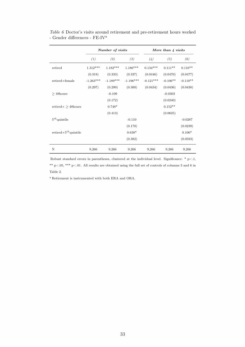
Table 6 Doctor’s visits around retirement and pre-retirement hours worked- Gender differences - FE-IVa


(1) (2) (3) (4) (5) (6)

retired 1.312*** 1.182*** 1.186*** 0.134*** 0.111** 0.116**

(0.318) (0.333) (0.337) (0.0446) (0.0470) (0.0477)

retired×female -1.263*** -1.189*** -1.196*** -0.121*** -0.106** -0.110**

(0.297) (0.299) (0.300) (0.0434) (0.0436) (0.0438)

≥ 48hours -0.109 -0.0303

(0.172) (0.0240)

retired× ≥ 48hours 0.748* 0.152**

(0.413) (0.0625)

5thquintile -0.110 -0.0287

(0.170) (0.0239)

retired×5thquintile 0.638* 0.106*

(0.382) (0.0593)

N 9,266 9,266 9,266 9,266 9,266 9,266

Robust standard errors in parentheses, clustered at the individual level. Significance: * p<.1,

** p<.05, *** p<.01. All results are obtained using the full set of controls of columns 3 and 6 in

Table 2.


33

Table 7 Number of General practitioner’s and Specialist’s visits - FE-IVa

General Practitioner Specialist

(1) (2) (3) (4) (5) (6)

retired 0.333 0.218 0.235 0.0711 0.0761 0.0702

(0.254) (0.268) (0.272) (0.0557) (0.0591) (0.0597)

age 0.00665 0.00856 0.00550 -0.0331 -0.0332 -0.0330

(0.118) (0.118) (0.117) (0.0237) (0.0238) (0.0237)

≥ 48hours -0.135 0.0272

(0.151) (0.0334)

retired× ≥ 48hours 1.069** 0.00669

(0.416) (0.0830)

5thquintile -0.212 0.0246

(0.142) (0.0324)

retired×5thquintile 0.839** 0.0141

(0.391) (0.0811)

poor health 0.546*** 0.541*** 0.540*** 0.104*** 0.104*** 0.104***

(0.125) (0.125) (0.125) (0.0224) (0.0224) (0.0224)

diagnosed conditions (sum) 0.278*** 0.277*** 0.278*** 0.0528*** 0.0528*** 0.0528***

(0.0492) (0.0492) (0.0492) (0.00927) (0.00928) (0.00928)

depression index 0.0912*** 0.0917*** 0.0914*** 0.00594 0.00598 0.00596

(0.0264) (0.0264) (0.0264) (0.00468) (0.00469) (0.00469)

N 7,486 7,486 7,486 7,486 7,486 7,486


p<.01. All results are obtained using the full set of controls of columns 3 and 6 in Table 2 and the restricted

sample from waves 1, 2 and 4.


34

7 Appendix

35

FigureA1Sh

areof

retirees

andnewly

retiredacross

coun

tries-Fe

males

36

FigureA2Sh

areof

retirees

andnewly

retiredacross

coun

tries-Males

37

Table A1 Early and Ordinary Retirement ages across countries

Country ERAa,b ORAa Effective Retirement Age

Men Women Men Women Men Women

Austria 62 57 65 60 62.1 59.6Germany 63 63 65 65 64.8 62.7Sweden 65 65 65 65 66.0 65.9Netherlands 65 65 65 65 63.8 64.1Spain 63 63 65 65 65.1 62.9Italy 61 61 65 62 62.4 61.6France 60 60 65 65 61.1 61.9Denmark 60 60 65 65 63.9 63.7Switzerland 63 62 65 64 65.3 64.5Belgium 60 60 65 65 61.8 61.0

a Early and Ordinary Retirement ages refer to individuals retiring in 2012 and are provided byOECD (2013), Gruber and Wise (2010); Hamblin (2013). ERA and ORA are defined for eachcountry according to the year of retirement of individuals and the minimum and full statutoryages in force at that time; early retirement ages are obtained from minimum statutory agesand, for some countries (see country profiles below), they are adjusted according to contributionrequirements and actuarial reductions.b Country profiles for ERA:Austria: early retirement in Austria was possible from the age of 55 for women and 60 formen until 2004. The 2004 reform introduced a gradual increase in ERA for both men andwomen born before 1943 and 1948, respectively. For individuals belonging to those cohorts andaffected by the reform, we set ERA accordingly.Germany: early retirement in Germany was possible from the age of 60 until 2003; after the2004 reform, early retirement is possible from age 63 for men and 62 women (63 from 2006).Sweden: the 1994 reform of the pension system in Sweden introduced a notional defined con-tribution scheme with no fixed-retirement age. Retirement is possible from age 61 in the publicpension scheme, but with automatic actuarial reductions depending on the age of retirement,on individual contributions and on the demographic and macroeconomic environment. So, theminimum pension age by itself is not binding enough to generate a discontinuity in the proba-bility of retirement. Moreover, the income-tested guaranteed pension cannot be claimed beforeage 65. Finally, in our sample less than 1% of retirees actually retire at 61 or earlier (with amedian above 65). For these reasons we consider ERA as not binding in Sweden.The Netherlands: early retirement in the Netherlands was possible from the age of 60 until1995, 61 until 2004, and in 2005 the Dutch early-retirement scheme was abolished.Spain: early retirement in Spain was possible from age 60 until 2001; in 2002 a reform shiftedthe minimum age to 61 and significantly increased reductions for workers voluntarily leavingthe labor market before age 65 (so that those who would stop working at 61 would have in-curred a reduction of 24-32%). Taking into account minimum age, years of contribution andrelated reductions, we set ERA at 63 for individuals retiring from 2002 onward.Italy: under the system in force before 2008, workers could retire at age 57 if they had con-tributed to the system for 35 years, while the reform approved in 2008 introduced a quotasystem based on a combination of age and seniority that increases the minimum age graduallyfrom 58 to 61 by 2013. Based on the combination of age and years of contributions we set ERAto 58 for men and 59 for women (who are more likely to have interrupted their careers) whoretired until 2008, and then to 60 between 2009 and 2011 and 61 until 2012. The 2011 reformabolished the quota system, making retirement possible without penalty from age 62, with atleast 42 years of contribution (in force from 2013).France: early retirement in France is possible from the age of 60.Denmark: early retirement in Denmark is being phased out but it is still available to workersborn before January 1st, 1959 (our whole sample) and to workers aged 60 to 65 who continueworking for 12 to 30 hours a week.Switzerland: early retirement was possible two years before the standard retirement age, i.e.from 63 for men and 62 for women since 2000. Until 2000 for women and 1997 for men, retire-ment was possible only at the standard age (65 for men, 63 for women), and for men retiringbetween 1997 and 2000 early retirement eligibility age was 64.Belgium: early retirement in Belgium was possible from the age of 60 for men and 55 for womenuntil 1987; after 1987 the minimum statutory age for early retirement for both men and womenhas been set at 60.

38

Table A2 Description and means of control variables

Variable Description Mean

Whole Sample Employed Retired

Occupations 1-digit ISCO-88ISCO 1 - Managers 0.125 0.132 0.116ISCO 2 and 3 - Professionals and Technicians 0.408 0.422 0.393ISCO 4 - Clerks 0.139 0.139 0.139ISCO 5 - Service workers 0.111 0.131 0.088ISCO 6 and 7 - Crafts & Trade workers 0.096 0.076 0.12ISCO 8 - Plant & Machine operators 0.049 0.034 0.065ISCO 9 - Elementary occupations 0.072 0.066 0.079

Industries 1-digit NACEAgriculture and mining 0.024 0.021 0.028Manufacturing 0.189 0.141 0.244Construction 0.062 0.064 0.059Wholesale, Hotels and Transports 0.148 0.134 0.165Financial and Real Estate services 0.111 0.109 0.112Public Administration 0.104 0.111 0.096Education, Health and other Services 0.361 0.419 0.296

Weekly hours worked≥ 48hours dummy = 1 if respondent works at least 48 0.149 0.142 0.123

hours a week (when employed)5thquintile dummy = 1 if respondent’s hours worked are 0.159 0.153 0.135

in the upper quintile of the weekly distribution

Incomedifficulty dummy = 1 if Household makes ends meet 0.187 0.154 0.226

with difficulty or great difficultyHousehold’s income deciles

1 0.046 0.044 0.0472 0.044 0.026 0.0653 0.062 0.045 0.0814 0.08 0.064 0.0985 0.093 0.072 0.1186 0.114 0.099 0.1317 0.13 0.132 0.1278 0.142 0.16 0.1219 0.149 0.183 0.1110 0.141 0.176 0.102

N 9,266 4,953 4,313

39

Table A3 Doctor’s visits around retirement - No health controls - FE-IV


(1) (2) (3) (4) (5) (6)

retired 0.531* 1.071** 0.679** 0.0510 0.133** 0.0735*(0.310) (0.443) (0.283) (0.0432) (0.0613) (0.0402)

age -0.000793 -0.0170 -0.00525 0.00630 0.00383 0.00562(0.142) (0.143) (0.142) (0.0207) (0.0208) (0.0207)

Demographics X X X X X XIndustry and Occupation X X X X X XIncome X X X X X X



First stage resultsAbove ERA 0.368*** 0.314*** 0.368*** 0.314***

(0.0146) (0.0153) (0.0146) (0.0153)Above ORA 0.264*** 0.160*** 0.264*** 0.160***

(0.0148) (0.0146) (0.0148) (0.0146)

R2 0.4275 0.3802 0.4451 0.4275 0.3802 0.4451F-stat of excluded instruments 634.89 315.51 410.92 634.89 315.51 410.92

N 9,266 9,266 9,266 9,266 9,266 9,266

Robust standard errors in parentheses, clustered at the individual level. Significance: * p<.1, ** p<.05,*** p<.01. All results are obtained using the set of controls as in columns 2 and 5 in Table 2.Hansen J statistic for overidentification is 1.341 (p = 0.2468) for column 3 and 1.741 (p = 0.1871) forcolumn 6.

40

Table A4 Alternative definitions of retirement FE-IV


(1) (2) (3) (4) (5) (6)

Panel A - Year/month of retirement

retireda 0.613** 0.522* 0.521* 0.0726* 0.0598 0.0625(0.259) (0.270) (0.272) (0.0375) (0.0394) (0.0397)

≥ 48hours -0.0824 -0.0353(0.173) (0.0250)

retired× ≥ 48hours 0.866** 0.146**(0.412) (0.0629)

5thquintile -0.0895 -0.0326(0.169) (0.0246)

retired×5thquintile 0.786** 0.117**(0.387) (0.0598)

First stage resultsb

Above ERA 0.330*** 0.333*** 0.334*** 0.330*** 0.333*** 0.334***(0.0161) (0.0169) (0.0169) (0.0161) (0.0169) (0.0169)

Above ORA 0.191*** 0.170*** 0.166*** 0.191*** 0.170*** 0.166***(0.0155) (0.0159) (0.0159) (0.0155) (0.0159) (0.0159)


N 8,730 8,730 8,730 8,730 8,730 8,730

Panel B - Self-reported retirement and no work performed

retiredc 1.238*** 1.124*** 1.104** 0.159*** 0.134** 0.133**(0.415) (0.431) (0.433) (0.0592) (0.0617) (0.0620)

≥ 48hours -0.161 -0.0360(0.179) (0.0246)

retired× ≥ 48hours 1.106 0.259**(0.793) (0.121)

5thquintile -0.169 -0.0350(0.178) (0.0245)

retired×5thquintile 1.139 0.246**(0.749) (0.115)

First stage resultsb

Above ERA 0.226*** 0.229*** 0.229*** 0.226*** 0.229*** 0.229***(0.0154) (0.0160) (0.0160 (0.0154) (0.0160) (0.0160)

Above ORA 0.161*** 0.145*** 0.143*** 0.161*** 0.145*** 0.143***(0.0155) (0.0156) (0.0155) (0.0155) (0.0156) (0.0155)


N 7,821 7,821 7,821 7,821 7,821 7,821

Robust standard errors in parentheses, clustered at the individual level. Significance: * p<.1, ** p<.05,*** p<.01. All results are obtained using the full set of controls of columns 3 and 6 in Table 2.a Year/month of retirement is used to define retirement status. Individuals are considered to be retired ifthe year/month of the interview is larger or equal to the year/month of retirement - i.e. the individualhas been retired for at least one month.b Hansen-J statistic for overidentification rejects the null hypothesis in all estimates.c We consider an individual as retired only if he reports to be retired and did not do any paid work duringthe 2 weeks preceding the interview.

Table A5 Alternative sample and specifications - coefficient on the retired vari-able - FE-IVa

Number of visits More than 4 visits Obs.

1. Drop countries:range [min;max]b [0.571**-0.943***] [0.0730*- 0.110**] [7,990-9,333]2. Country-specific time trends 0.766*** 0.0898** 9,266

(0.274) (0.0392)3.Country-specific age trends 0.761*** 0.0892** 9,266

(0.274) (0.0392)

Robust standard errors in parentheses, clustered at the individual level. Significance: * p<.1, **p<.05, *** p<.01.a Retirement is instrumented with both ERA and ORA.b The range of estimates is obtained excluding one country at a time from our preferred specification.

41

Table A6 Dynamic IV

Number of visits (t+1) More than 4 visits (t+1)

retired(t, t+ 1) 0.710* 0.0927*(0.413) (0.0560)

number of visits(t) 0.311***(0.0212)

>4 visits (t) 0.239***(0.0187)

age 0.00554 0.000520(0.0218) (0.00293)

female 0.212** 0.0172(0.108) (0.0144)

poor health(t) 0.292* 0.0347(0.168) (0.0217)

diagnosed conditions(t) 0.419*** 0.0454***(0.0553) (0.00740)

mental health index(t) 0.0434 0.00723*(0.0282) (0.00396)

R2 0.199 0.128N 4,747 4,747

Robust standard errors in parentheses, clustered at the individual level. Significance: * p<.1, ** p<.05,*** p<.01. All results are obtained using the full set of controls of columns 3 and 6 in Table 2.First-stage statistics for both models confirm the relevance of the instruments. However, the overiden-tification test for the equation of the number of visits is rejecting the null with a p-value of 0.083.

42

Is there a Retirement-Health Care utilization puzzle ...

Documents

Transcript of Is there a Retirement-Health Care utilization puzzle ...