Is .5529.1.1985-Permeability Tests

Disclosure to Promote the Right To Information

Whereas the Parliament of India has set out to provide a practical regime of right to information for citizens to secure access to information under the control of public authorities, in order to promote transparency and accountability in the working of every public authority, and whereas the attached publication of the Bureau of Indian Standards is of particular interest to the public, particularly disadvantaged communities and those engaged in the pursuit of education and knowledge, the attached public safety standard is made available to promote the timely dissemination of this information in an accurate manner to the public.

इंटरनेट मानक

“!ान $ एक न' भारत का +नम-ण”Satyanarayan Gangaram Pitroda

“Invent a New India Using Knowledge”

“प0रा1 को छोड न' 5 तरफ”Jawaharlal Nehru

“Step Out From the Old to the New”

“जान1 का अ+धकार, जी1 का अ+धकार”Mazdoor Kisan Shakti Sangathan

“The Right to Information, The Right to Live”

“!ान एक ऐसा खजाना > जो कभी च0राया नहB जा सकता है”Bhartṛhari—Nītiśatakam

“Knowledge is such a treasure which cannot be stolen”

“Invent a New India Using Knowledge”

है”ह”ह

IS 5529-1 (1985): Code of practice for in-situ permeabilitytest, Part 1: Test in overburden [WRD 5: GelogicalInvestigation and Subsurface Exploration]

© BIS 2013

B U R E A U O F I N D I A N S T A N D A R D SMANAK BHAVAN, 9 BAHADUR SHAH ZAFAR MARG

NEW DELHI 110002

March 2013 Price Group 9

IS 5529 (Part 1) : 2013

Hkkjrh; ekud

LoLFkkus HksFkrk ijh{k.k

Hkkx Hkkx Hkkx Hkkx Hkkx 1 vksojcMZu esa ijh{k.k vksojcMZu esa ijh{k.k vksojcMZu esa ijh{k.k vksojcMZu esa ijh{k.k vksojcMZu esa ijh{k.k — jhfr lafgrkjhfr lafgrkjhfr lafgrkjhfr lafgrkjhfr lafgrk

¼ nwljk iqujh{k.k ½

Indian Standard

IN-SITU PERMEABILITY TESTS

PART 1 TESTS IN OVERBURDEN — CODE OF PRACTICE

( Second Revision )

ICS 93.020

Geological Investigations and Subsurface Exploration Sectional Committee, WRD 5

FOREWORD

This Code (Part 1) (Second Revision) was adopted by the Bureau of Indian Standards, after the draft finalized by

the Geological Investigations and Subsurface Exploration Sectional Committee had been approved by the Water

Resources Division Council.

This Code was first published in 1969 and revised in 1985. The present revision is proposed to reflect the experience

gained on the subject since then.

Field permeability of subsurface strata is necessary in connection with various engineering problems, such as

design of cut-off for earth dam, calculation of pumping capacity for dewatering excavations and determination of

aquifer constants of subsurface strata.

The field permeability tests are carried out to determine permeability of each subsurface strata encountered up to

bed rock as well as to ascertain overall permeability of strata. The tests are carried out in standard drill holes

where subsurface explorations for foundations are carried out by drilling. The tests are also carried out in auger

holes or bore holes of larger size than those made by standard drill rods. These tests are convenient and reliable

for depth up to 30 m and they dispense with costly drilling operations. The tests carried out are either pumping in

or pumping out type. When the stratum being tested is above water table, the pumping in test is carried out and

when it is below water table then either pumping in or pumping out test may be conducted.

The coefficient of permeability is usually evaluated on the basis of Darcy’s law which states that the rate of flow

through a porous medium is proportional to the hydraulic gradient. This relationship is applicable for steady and

laminar flow through saturated soils. A reliable determination of permeability may be made only when the above

conditions for the validity of Darcy’s law are fulfilled. Further, the reliability of the values of permeability

depends upon the homogeneity of the strata tested and on the validity of the following assumptions in the formula

used:

a) Non-pumping piezometer surface is horizontal; and

b) Non-pumping aquifer is horizontal, of uniform saturated thickness, of infinite aerial extent and is

homogeneous.

This Code is published in two parts. Other part in the series is:

Part 2 Test in bedrock

For the purpose of deciding whether a particular requirement of this standard is complied with, the final value,

observed or calculated, expressing the result of a test or analysis, shall be rounded off in accordance with IS 2 : 1960

‘Rules for rounding off numerical values (revised)’. The number of significant places retained in the rounded off

value should be the same as that of the specified value in this standard.

1

IS 5529 (Part 1) : 2013

Indian Standard

IN-SITU PERMEABILITY TESTS

PART 1 TESTS IN OVERBURDEN — CODE OF PRACTICE

( Second Revision )

1 SCOPE

1.1 This Code (Part 1) specifies the methods, as

mentioned in 1.2 and 1.3 out of a number of methods,

of determining field permeability in overburden. These

are more commonly adopted for civil engineering

purposes.

1.2 Pumping in Tests (Gravity Feed in Drill Holes

or Bore Holes)

a) Constant head method (cased well, open end

test);

b) Falling head method (uncased well); and

c) Slug method.

1.3 Pumping Out Tests

a) Unsteady state;

b) Steady state; and

c) Bailor method.

2 TERMINOLOGY

For the purpose of this standard, the following

definitions shall apply.

2.1 Coefficient of Permeability — The rate of flow

of water under laminar flow conditions through a unit

cross-sectional area of a porous medium under a unit

hydraulic gradient and at a standard temperature of

27°C.

2.1.1 As it is not possible to control the temperature in

the field to 27°C, the coefficient of permeability K27,

at 27°C is calculated by the following formula:

K27

= t t

27

Kh

h

where

ηt = viscosity of water at the field temperature,

t;

Kt = coefficient of permeability at the field

temperature, t; and

η27 = viscosity of water at 27°C.

2.2 Coefficient of Storages — It is defined as the

volume of water that a unit decline in head releases

from storage in a vertical column of the aquifer of unit

cross-sectional area and is given by the following

formula:

S = n b γw

+ aÊ ˆÁ ˜Ë ¯

b

h

where

η = porosity of sand;

γw = unit weight of water;

b = aquifer thickness;

β = compressibility of water or reciprocal of its

bulk modulus of elasticity; and

α = vertical compressibility of the solid skeleton

of the aquifer.

2.3 Coefficient of Transmissivity (T) — It is defined

as the rate of flow of water through a vertical strip of

aquifer of unit width under a unit hydraulic gradient.

It characterizes the ability of the aquifer to transmit

water and is given by the following formula:

T = Kb

where

K = coefficient of permeability; and

b = aquifer thickness.

2.4 Constant Head Method — The method in which

the water level in the test hole is maintained constant

and the permeability is computed from the data of

steady state constant discharge.

2.5 Falling Head Method — The method in which

the water level in the test hole is allowed to fall and the

equivalent permeability is computed from the data of

the rate of fall of the water level.

2.6 Slug Method — The test done by instantaneous

injection of a given quantity of ‘slug’ of water into a

well, and determining the coefficient of permeability

from the fall of water level.

2.7 Bailor Method — The test done by instantaneous

bailing of water from a well and determining the

coefficient of permeability from the data of the

recovery of water level.

2

IS 5529 (Part 1) : 2013

3 PUMPING IN TEST

3.1 Applicability

3.1.1 The pumping in test is applicable for strata in both

cases of above and below water table. The test is

especially performed in formations of limited thickness.

The tests give permeability of the material in the

immediate vicinity of the bottom of the drill hole. It

may thus be used for determining the permeability of

different layers in stratified foundations and thus check

the effectiveness of grouting in such formulations. This

method is economical and do not require elaborate

arrangements required for the pump out tests.

3.1.2 Limitations

3.1.2.1 In the pumping in test method water is fed from

outside and, therefore, the test results are likely to be

affected by the thin film formed by the sedimentation

of suspended fines present in the water.

3.1.2.2 The method does not provide the overall

permeability of the strata but the permeability of a

stratum of thickness five times the diameter of the hole

below and above the level of casing.

3.2 Constant Head Method (Cased Well-Open End

Test)

3.2.1 The constant head method is used when the

permeability of the strata being tested is high.

3.2.2 Equipment

3.2.2.1 Drilling or boring set or auger, required for

excavating a bore hole.

3.2.2.2 Driving pipe casing or blind pipe, of length

equal to the depth up to which testing is to be done.

3.2.2.3 Pumped water supply or a number of drums of

200 litre capacity full of water

The number of drums depends upon the expected water

percolation. One drum should have a regulating valve

at the bottom and an overflow in the form of sharp

crest at the top.

3.2.2.4 Delivery hose pipe or rubber tubing, of 12 mm

diameter fitted with a regulating cock.

3.2.2.5 Arrangements for measuring water level in the

test holes like a mason’s plumb with a measuring tape

of preferably an electric probe as described in 3.2.2.6.

3.2.2.6 The electric probe (see Fig. 1) consists of a

long wire kept straight by means of a weight tied at

the bottom end. This probe should be connected to a

cell and galvanometer. A connecting wire passes from

the other terminal of the galvanometer to earth. It may

be tied to the metal casing of the observation well itself.

Then galvanometer needle will show deflection on

completion of the electric circuit when the probe

touches water in the hole. The depth of the electric

wire lowered is measured by tape or by the graduations

FIG. 1 SET-UP FOR CONSTANT HEAD METHOD (GRAVITY FEED, OPEN-END TYPE)

3

IS 5529 (Part 1) : 2013

marked on the electric wire itself for determining the

depth of water level in the hole.

3.2.2.7 Miscellaneous equipment, stop watches,

graduated cylinders pressure gauges, water meter and

enamelled bucket for measuring discharge.

3.2.3 Procedure

3.2.3.1 In this method, a hole should be drilled or bored

up to the level at which the test is to be performed. The

casing should be sunk by drilling and driving or jetting

with water and driving, whichever gives the tightest fit

to the casing in the hole. The casing should be

simultaneously driven as the drilling or boring of the

hole is in progress. After the required level is reached,

the hole should be cleaned by means of scooping

spoons and bailor. If the hole extends below ground

water level, the hole should be kept full of water while

cleaning it (as otherwise, due to water pressure, soil

may squeeze into the bottom of the casing pipe) and

should be cleaned by passing air under pressure by air

jetting method.

3.2.3.2 After the hole is cleaned the test should be

started by allowing clean water through a metering

system to maintain gravity flow at constant head. The

flow should be adjusted by the regulating valve in such

a way so as to obtain steady water level in the hole. In

the tests above water table, a stable constant level is

rarely obtained, and a surging of the level within 20 mm

to 30 mm at a constant rate of flow for about 5 min

may be considered satisfactory.

3.2.3.3 For measuring water level or constant water

level maintained in the hole during test, the naked point

of the enamelled wire of the electric probe should be

lowered in the hole till it touches the water level. The

observations of the water level at 5 min intervals should

be noted. When three consecutive readings show

constant values, further observations may be stopped

and the constant reading should be taken to the depth

of water level. Alternatively, the water reading may also

be taken by means of soundings by mason’s plumb.

3.2.4 Observations

The observations of the test should be recorded suitably.

A recommended proforma for the record of results is

given in Annex A.

3.2.5 Computations of Coefficient of Permeability

3.2.5.1 The permeability by constant head method

(open-end test) should be obtained from the following

relation determined by electrical analogy experiments:

5.5

QK

rH= … (1)

where

K = coefficient of permeability;

Q = constant rate of flow into the hole;

r = internal radius of casing; and

H = differential head of water = H1 (gravity head)

– Hf (head loss due to friction).

NOTES

1 The value of H, for gravity test made below water table is the

difference between the level of water in the casing and the

ground water level. For test above water table, H1 is the depth

of water in the hole as shown in Fig. 2.

2 The value of Hf (head loss due to friction) may be obtained

from Fig. 3 and Fig. 4 for EX, AX, BX and NX size rods.

3.2.5.2 When K is measured, in cm/s, Q, in litre/min,

and H, in m, equation (1) may be written as:

K = C1 × Q/H

FIG. 2 CONSTANT HEAD METHOD — PUMPING IN TYPE (GRAVITY FEED, OPEN-END TEST)

4

IS 5529 (Part 1) : 2013

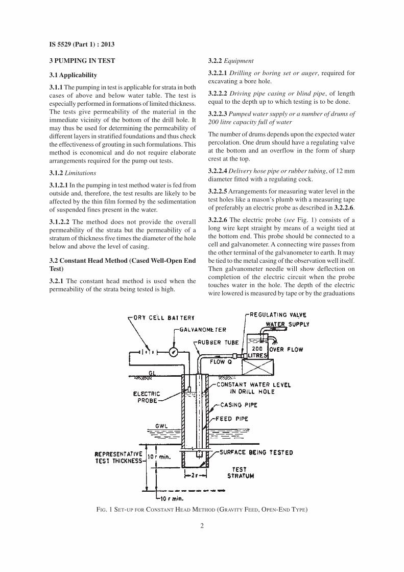
FORMULA USED

�2 2

f

[ /( /4)]

2

fl Q dH

d g= ¥

where

Hf = head loss Q = discharge

f = friction constant l = length of rod

d = inside diameter of rod g = acceleration due to gravity

FIG. 3 HEAD LOSS DUE TO PIPE FRICTION FOR NX SIZE RODS PER 3 m LENGTH OF DRILL ROD VERSUS DISCHARGE

5

IS 5529 (Part 1) : 2013

FORMULA USED

�2 2

f

[ /( /4)]

2

fl Q dH

d g= ¥

where

Hf = head loss d = inside diameter of rod

l = length of rod Q = discharge

f = friction constant g = acceleration due to gravity

FIG. 4 HEAD LOSS DUE TO PIPE FRICTION FOR EX, AX AND BX SIZE RODS PER 3 m LENGTH

OF DRILL ROD VERSUS DISCHARGE

6

IS 5529 (Part 1) : 2013

Values of C1, which vary with the size of casing and

rods, are given in Table 1.

3.2.5.3 An example illustrating the use of the formula

is given below:

Given NX casing

Q = 40 1/min

H1 = gravity = 2.63 m

Hf = using NX rod at 40 1/min = 0.001 3 m (from

Fig. 3) = 0.001 3 m per 3 m section

Distance from top to bottom of pipe = 3 m

Hf =3

0.001 3 × = 0.001 3 m3

H = H1 – Hf = 2.63 m – 0.001 3 m = 2.63 m. The

value of C1 for NX casing (from Table 1) =

7.95 ×10 -3

Hence

K = C1 (Q/H) =

37.95 10 40

2.63

-¥ ¥ = 120.91 × 10-3 cm/s

3.2.6 Precautions

3.2.6.1 Water level in the test hole shall be recorded

before the permeability tests are started.

3.2.6.2 The hole should be thoroughly flushed with

clear water before the tests are commended.

3.2.6.3 The water used for the tests should be clear

and free from silt.

3.2.6.4 It is desirable that the temperature of the added

water is higher than ground water temperature.

3.3 Falling Head Method

3.3.1 The test may be conducted both above and below

water table but is considered more accurate below water

table. It is applicable for strata in which the hole below

the casing pipe can stand and has low permeability;

otherwise the rate of fall of the head may be so high

that it may be difficult to measure.

3.3.2 Equipment

3.3.2.1 All the equipment listed in 3.2.2.

3.3.2.2 Pneumatic mechanical or any other suitable type

packers of the diameter of the hole and length when

expanded shall be equal to five times the diameter of

the hole.

3.3.2.3 A perforated pipe of suitable length. The test

set up is shown in Fig. 5.

3.3.3 Procedure

The hole should be drilled or bored up to the bottom of

the test horizon and cleaned by the method described

in 3.2.3.1. After cleaning the hole, the packer should

be fixed at the desired depth so as to enable the testing

of the full section of the hole below the packer. In

conducting packer tests standard drill rods should be

used. The water pipe should be filled with water up to

its top and the rate of fall of the water inside the pipe

FIG. 5 SET-UP FOR FALLING HEAD METHOD

Table 1 Values of C1 (× 10-3)

(Clause 3.2.5.2)

Sl

No.

(1) (2) (3) (4) (5) (6) (7)

i) Size of casing EX AX BX NX

ii) Diameter of hole (2r), in mm 38.1 48.4 60.3 76.2 100 150 200

iii) C1 (× 10-3) 15.90 12.50 10.0 7.95 6.06 4.04 3.03

7

IS 5529 (Part 1) : 2013

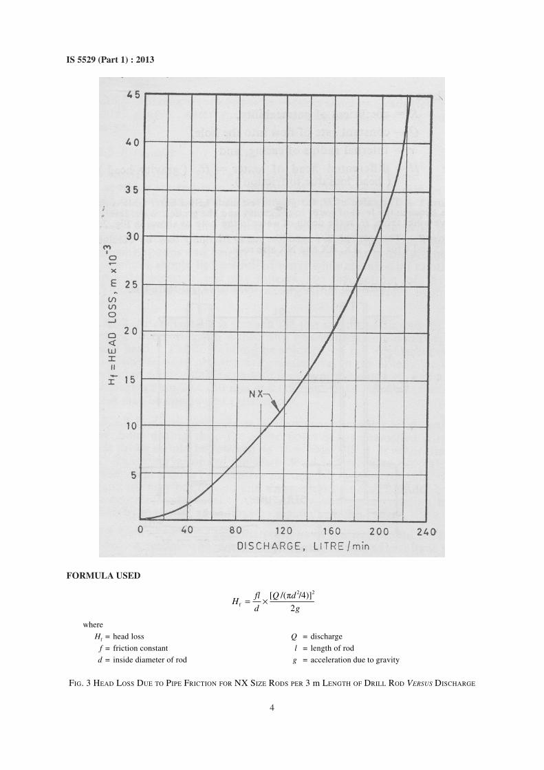
should be recorded. If the hole cannot stand as such

then casing pipe with perforated section in the strata to

be tested should be used.

3.3.4 Observations


A recorded proforma for the record of results is given

in Annex B.

3.3.5 Computations of Coefficient of Permeability

3.3.5.1 The permeability by falling head method in an

uncased hole should be computed by the following

relations:

2

e 1 2

e

2 1

log /(log )

8

h hd LK

R t tL=

-…. (2)

where

K = coefficient of permeability;

d = diameter of intake pipe (stand pipe);

L = length of test zone;

h1 = head of water in the stand pipe at time t1,

above piezometeric surface;

h2 = head of water in the stand pipe at the time

t2, above piezometeric surface; and

R = radius of hole.

3.3.5.2 The formula is based on the following

assumptions:

a) The soil stratum is homogeneous and the

permeability of soil is equal in all directions;

and

b) The soil stratum in which the intake point is

placed is of infinite thickness and that artesian

conditions does not prevail.

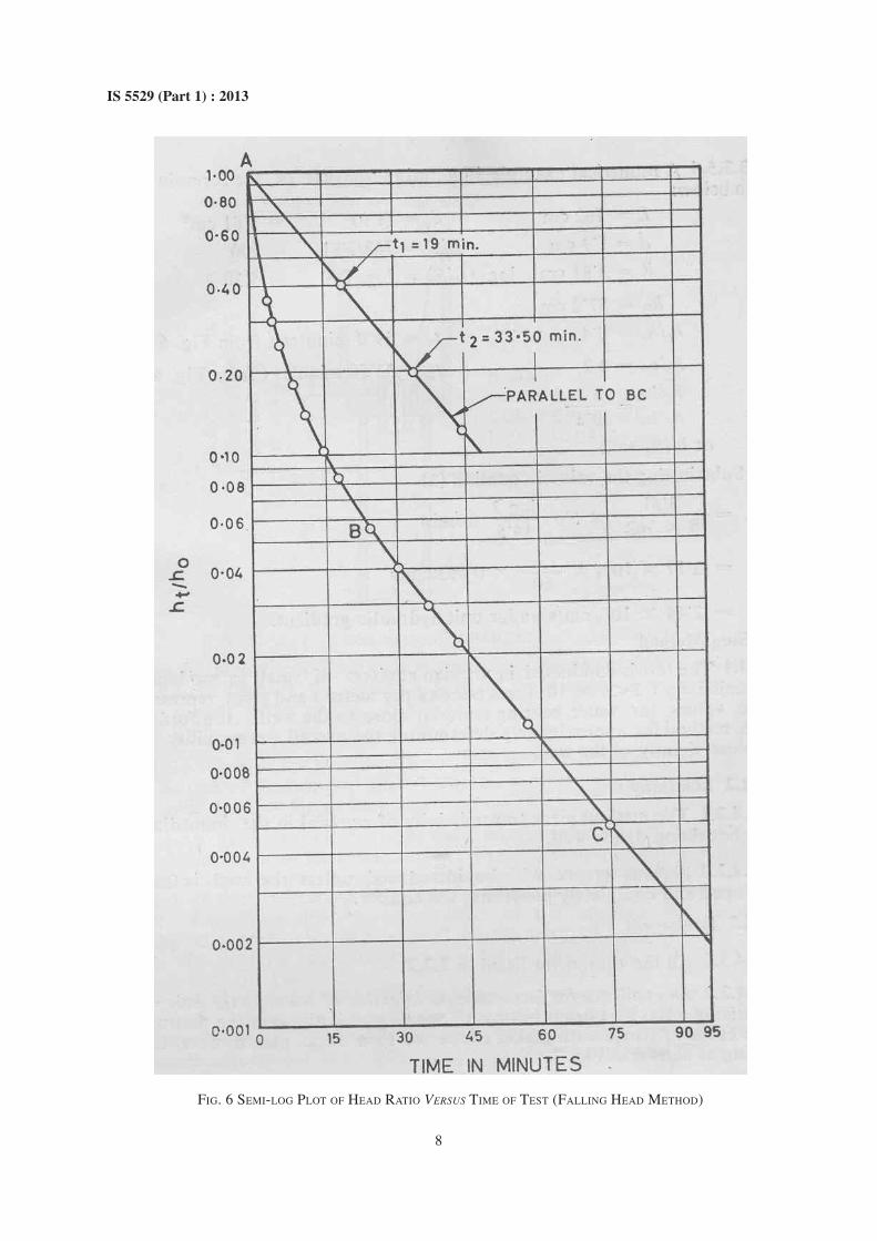
3.3.5.3 The head ratio ht/h0 (where ht = head of water

in the stand pipe at any time t and h0 = depth of static

water level at time t0) versus time curve should be

plotted on the semilog plot as shown in Fig. 6. The

curve shows pronounced initial curvature whereas after

a time lag of about 20 min, the curve is straight. A

straight line through the origin and parallel to the

straight portion of the curve should be drawn to

represent a steady state of flow into the test strata. The

value of h1/h0 and h2/h0 corresponding to time t1, and t2

respectively is read from the graph. The value h1/h2

corresponding to time t1 and t2 is calculated and

substituted in equation (2) to obtain the coefficient of

permeability.

3.3.5.4 A numerical example illustrating the use of the

formula is given below:

L = 762 cm d2 = (1.9)2 = 3.61 cm2

d = 1.9 cm L/R = 762/3.81 = 200

R = 3.81 cm loge(L/R) = loge 200= 5.30

h0 = 57.2 cm

h1/h0 = 0.4 t1 = 19.0 min (from Fig. 6)

h2/h0 = 0.2 t2 = 33.50 min (from Fig. 6)

1 0

2 0

/ 0.4

/ 0.2

h h

h h=

or h1/h2 = 2

Substituting the value in equation (2)

= e3.61 log .2

5.3 cm / min8 762 14.5

¥¥

= 2.17 × 10-4 × 1

0.693 cm/s60

¥

= 2.48 × 10-6 cm/s under unit hydraulic gradient.

3.4 Slug Method

3.4.1 The test is conducted in artesian aquifers of small

to moderate transmissivity (T< 6 × 105l/day/m) and

gives representative values for water bearing material

close to the well. It affords a quick method for

approximately determining the overall permeability in

the close vicinity of the well.

3.4.2 Limitations

3.4.2.1 The method gives transmissivity of material in

the immediate neighbourhood of the well.

3.4.2.2 Serious errors shall be introduced unless the

well is fully developed and completely penetrates the

aquifer.

3.4.3 Equipment

3.4.3.1 All the equipment listed in 3.2.2.

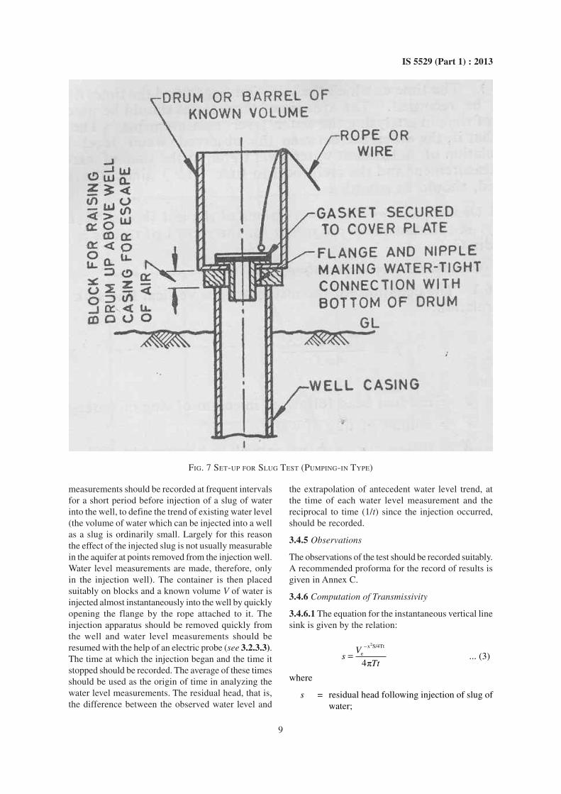
3.4.3.2 An appliance for instantaneous injection of

water in the hole, comprising a 200 litre drum having

an opening with nipple at the bottom and a cover of

flange with gasket connected to a rope placed over the

opening as shown in Fig. 7.

3.4.3.3 Blocks

Fifteen centimetre high to be placed below the

container (see 3.4.3.2) to provide a vent for the escape

of air above the water surface in the well.

3.4.4 Procedure

3.4.4.1 In this method also, the drilling or boring of

the hole up to the bottom of the test horizon, sinking

the casing and cleaning the hole should be done by the

method described in 3.2.3.1.

3.4.4.2 After cleaning the hole, water level

8

IS 5529 (Part 1) : 2013

FIG. 6 SEMI-LOG PLOT OF HEAD RATIO VERSUS TIME OF TEST (FALLING HEAD METHOD)

9

IS 5529 (Part 1) : 2013

FIG. 7 SET-UP FOR SLUG TEST (PUMPING-IN TYPE)

measurements should be recorded at frequent intervals

for a short period before injection of a slug of water

into the well, to define the trend of existing water level

(the volume of water which can be injected into a well

as a slug is ordinarily small. Largely for this reason

the effect of the injected slug is not usually measurable

in the aquifer at points removed from the injection well.

Water level measurements are made, therefore, only

in the injection well). The container is then placed

suitably on blocks and a known volume V of water is

injected almost instantaneously into the well by quickly

opening the flange by the rope attached to it. The

injection apparatus should be removed quickly from

the well and water level measurements should be

resumed with the help of an electric probe (see 3.2.3.3).

The time at which the injection began and the time it

stopped should be recorded. The average of these times

should be used as the origin of time in analyzing the

water level measurements. The residual head, that is,

the difference between the observed water level and

the extrapolation of antecedent water level trend, at

the time of each water level measurement and the

reciprocal to time (1/t) since the injection occurred,

should be recorded.

3.4.5 Observations



given in Annex C.

3.4.6 Computation of Transmissivity

3.4.6.1 The equation for the instantaneous vertical line

sink is given by the relation:

�

2x S/4Tt

e

4

Vs

Tt

-

= ... (3)

where

s = residual head following injection of slug of

water;

10

IS 5529 (Part 1) : 2013

V = volume of slug of water;

X = distance from injection well to observation

well;

S = coefficient of storage;

T = coefficient of transmissivity; and

t = time since slug was injected.

3.4.6.2 For water level measurements in the injection

hole, x is replaced by the effective radius of the well

rw. For values of x as small as rw specially where S is

small, as for artesian aquifers, the exponent of e in

equation (3), approaches zero as t becomes large and

the value of the exponential term approaches unity.

Then if V is expressed in litre, T in litre per day per

metre, t in min and s in m, equation (3) may be written

in the form:

m114.6 ( .1/ )V tT

s= … (4)

where

tm = time following instantaneous injection of

slug of water.

3.4.6.3 The residual head (s) in metre should be plotted

against the reciprocal of the time, in minute since the

injection occurred (1/tm) as shown in Fig. 8. A straight

line drawn through the observed data should pass

through the origin (if the observed data from a slug

test do not fall on the straight line the observation well

may be sluggish and, if so, should be further

developed). An arbitrary point is picked on the straight

line and the corresponding values of l/tm and s should

be substituted in equation (4).

3.4.6.4 An example illustrating the use of equation (4)

is given below:

l/tm = 0.5 (see Fig. 8)

s = 0.05 (see Fig. 8)

V = 150 litre

T = 114.6 (v.1/tm) 114.6 150 0.5

0.05

¥ ¥=

= 171 900 litre/day/m

4 PUMPING OUT TESTS

4.1 Applicability

The pumping out test is an accurate method for finding

out in-situ permeability of the strata below water table

or below river bed. This method is best suited for all

ground water problems where accurate values of

permeability representative of the entire aquifer are

required for designing cut off or planning excavations.

4.2 Equipment

4.2.1 All the equipment listed in 3.2.2.

4.2.2 Water Meter, one impeller type water meter;

should be able to read up to 0.01 litre, to be tested

once in a month.

FIG. 8 RESIDUAL HEAD VERSUS RECIPROCAL OF TIME FOLLOWING THE INSTANTANEOUS OF SLUG OF WATER

11

IS 5529 (Part 1) : 2013

4.2.3 Pump Centrifugal/Turbine, of capacity 5 l/min

to 250 l/min and 250 l/min to l 600 l/min depending

upon the expected yield.

4.2.4 Well Pipe, one, 250 mm GI pipe having maximum

number of 25 mm dia holes over the portion below the

water table and having a wire mesh fixed on this

portion. The aperture of the wire mesh should be taken

as the diameter of 60 percent finer material of the

aquifer.

4.2.5 Piezometers or Observation Pipes, of 50 mm dia

extending to a depth depending upon the ground level

and the expected lowering of the ground water. It

should also have strainer (as in 4.2.4) along full length

except top 0.6 m.

4.2.6 The test arrangement is shown in Fig. 9 and

Fig. 10.

4.3 Procedure

4.3.1 The installation for pumping out test consists of

fully or partially penetrating well and suitable number

of piezometers arranged on 3 tiers preferably 120° to

each other. A 400 mm bore hole should be drilled by

using direct or reverse circulation methods of drilling

(based on prevailing geohydrological conditions)

extending to the bottom of the test section. Where the

total saturated thickness of the aquifer is very large

and drilling the hole to bottom of the aquifer is

expensive, partially penetrating well may be used. The

impervious boundary or bed rock should be ascertained

by drilling. Adjustment for partial penetration should

be made by Kozeny’s relation given in 4.3.5.

4.3.2 The well consists of 250 mm dia GI pipe having

maximum number of holes over the portion below the

water table and having wire mesh fixed around this

portion of the pipe. The aperture of the wire mesh shall

depend upon the grading of the surrounding aquifer

and should be taken as the diameter of 60 percent finer

material. A conical shoe at the bottom and a blind pipe

on the top, from water table to ground surface are

provided. A 75 mm thick coarse sand and travel filter

should be placed all round the screen to a height

approximately 3 m above the top of the screen. During

development of the well, there is a possibility of more

intake of coarse sand due to large quantities of finer

sands being pumped out. The shrouding should be

continued till the well yields sand free water.

4.3.3 For carrying out the test, the well should be first

pumped up to the depth for which the overall

permeability is to be determined. The pump should be

run at a constant rate of discharge continuously till the

pumped well attains equilibrium conditions in the

piezometer surface. This period varies from 10 h to

100 h depending upon the aquifer conditions, its

thickness, permeability and slope. The observation in

piezometers should be taken at suitable intervals of

time. In the initial stages, say for the first 15 min, the

observations may be taken at 30 s interval; for the next

30 min at 1 min interval; for the next 30 min at 2 min

interval and for the next 2 h at 5 min interval. After

this it may be increased to hourly and then to 5 hourly

and 10 hourly intervals till equilibrium conditions are

achieved. These intervals are only arbitrary and may

be changed to suit the site conditions. After completion

FIG. 9 PLAN SHOW ARRANGEMENT OF PUMPING WELL AND PIEZOMETERS FOR PUMPING

12

IS 5529 (Part 1) : 2013

of pumping out and shut down, observations for

recovery should be also continued and the two sets of

data, one during pumping out and the other during

recovery, should be used for analysis.

4.3.4 The discharge of the well during observations

should remain constant and is determined either by the

V-notch or trajectory method.

4.3.4.1 In the V-notch method the well flow is

discharged through a 5 m straight section of pipe and

fitted into a stilling chamber of V-notch arrangement.

The head over the notch should be measured. The water

passing through the V-notch should be collected into

the masonry collection chamber from where it is carried

through a pipe into a ditch or drain lined with polythene

plastic to prevent water from seeping into the sand

aquifer in the vicinity of the well. The ditch is sited at

least 150 m downstream of the V-notch. For a 90°

V-notch, discharge = 2.56 H5/2 where H is the head of

water over the notch.

4.3.4.2 Trajectory method

The water emerging from a pipe flowing full will follow

the ideal parabolic curve for a considerable distance;

hence the equation of a free jet may be used for

estimating the velocity at which water leaves the pipe

by measuring the jet coordinates. If the outlet pipe is

horizontal and referring to the mid-point of the outlet

as the origin, then the velocity at any point on the jet is

given by 0 / 2( )V X g Z= in which X and Z are the

horizontal and vertical coordinates of the point. Since

the pipe from which water is coming out is full of water,

the velocity multiplied by its cross-sectional area gives

the discharge for the pipe.

4.3.5 Adjustment for Partial Penetration

4.3.5.1 The formulae for the computation of coefficient

of transmissivity as mentioned in 4.5.1.1 and 4.5.1.2

are applicable only for fully penetrating wells. If the

well is partially penetrating then the adjustment for the

partial penetration of the aquifer is done. Kozeny

modified this theoretical formula for partial penetration

of wells. According to Kozeny, for equal values of

drawdown, if vertical permeability is equal to horizontal

permeability the relation between the values of

discharge in partially and fully penetrating wells is

given as below:

e

p f 1 7( cos2 2

rQ Q

b

Ï ¸apÔ Ô= a +Ì ˝aÔ ÔÓ ˛… (5)

where

Qp = constant rate of discharge for partially

penetrating well in l/min;

Qf = constant rate of discharge for fully

penetrating well in 1/min;

α = degree of partial penetration (that is ratio of

the length of the perforated section below

the initial water table to the full saturated

thickness of the unconfined aquifer);

FIG. 10 TYPICAL ARRANGEMENT FOR PUMPING OUT TEST

13

IS 5529 (Part 1) : 2013

re = effective radius of the pumping well, in m

(see Fig. 10); and

b = full saturated thickness of the aquifer, in m.

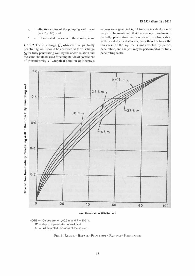
4.3.5.2 The discharge Qp observed in partially

penetrating well should be corrected to the discharge

Qf for fully penetrating well by the above relation and

the same should be used for computation of coefficient

of transmissivity T. Graphical solution of Kozeny’s

expression is given in Fig. 11 for ease in calculation. It

may also be mentioned that the average drawdown in

partially penetrating wells observed in observation

wells located at a distance greater than 1.5 times the

thickness of the aquifer is not effected by partial

penetration, and analysis may be performed as for fully

penetrating wells.

Well Penetration W/b Percent

NOTE — Curves are for re=0.3 m and R = 300 m.

W = depth of penetration of well; and

b = full saturated thickness of the aquifer.

FIG. 11 RELATION BETWEEN FLOW FROM A PARTIALLY PENETRATING

Rati

o o

f F

low

fro

m P

art

ially P

en

etr

ati

ng

Well t

o t

hat

fro

m F

ully P

en

etr

ati

ng

Well

14

IS 5529 (Part 1) : 2013

4.4 Observations



given in Annex D.

4.5 Computation of Coefficient of Transmissivity

The coefficient of transmissivity T is determined either

by the Theis unsteady state or non-equilibrium method

or by Theim’s steady state formula.

4.5.1 The unsteady state of non-equilibrium method is

applicable for confined aquifer only and for fully

penetrating wells. For unconfined aquifer, correction

as detailed in 4.5.4 may be carried out in the value of

drawdown s in an observation well and the same

formula as for confined case may be used.

4.5.1.1 The drawdown in an observation well in the

unsteady state is given by Theis’s well formula:

�

�

u

t

u4

Q es du

T u

-

= Ú ...(6)

where

s = drawdown in observation hole,

Qt = constant rate of discharge for fully

penetrating well,

e = base of natural logarithms = 2.718,

T = coefficient of transmissivity,

u =

2

4

r S

Tt,

r = distance of observation well from pumped

well,

S = coefficient of storage, and

t = time since pumping started.

Expressing Qt in 1/min and T in l/day/m:

± u

t

u

114.6 Q es du

T u

-

= Ú ….(7)

where

s = drawdown in the observation hole, in m;

u = 250 r2 S/Tt;

t = time since pumping started in days;

r = distance of observation well from pumped

well, in m;

S = coefficient of storage; and

T = coefficient of transmissivity in l/day/m.

4.5.1.2 The integral of equation (7) is a function of the

lower limit and is written as W (u), which is called well

function of u. It can be expanded in convergent series

given by:

W(u) = – 0.577 2 – loge u+ u

–

2 2

3 2! 3 3!

u u+

¥ ¥... (8)

4.5.1.3 Solution of the integral of equation (7) for T,

however, is relatively difficult since it occurs both inside

and outside the integral function. A graphical method of

superimposition devised by Theis makes it possible to

obtain a simple solution of equation (7). Substituting

the value of W (u) for the integral, equation (7) becomes:

S =

2

f

114.6 2500.5772 loge

r SQ

T Tt

ÈÍÍ- - +ÍÍÍÎ

2 32 2

2

250 250

250

2 2! 3 3!

r S r S

Tt Ttr S

Tt

˘Ê ˆ Ê ˆ˙Á ˜ Á ˜Ë ¯ Ë ¯ ˙+ - + ˙¥ ¥ ˙˙̊

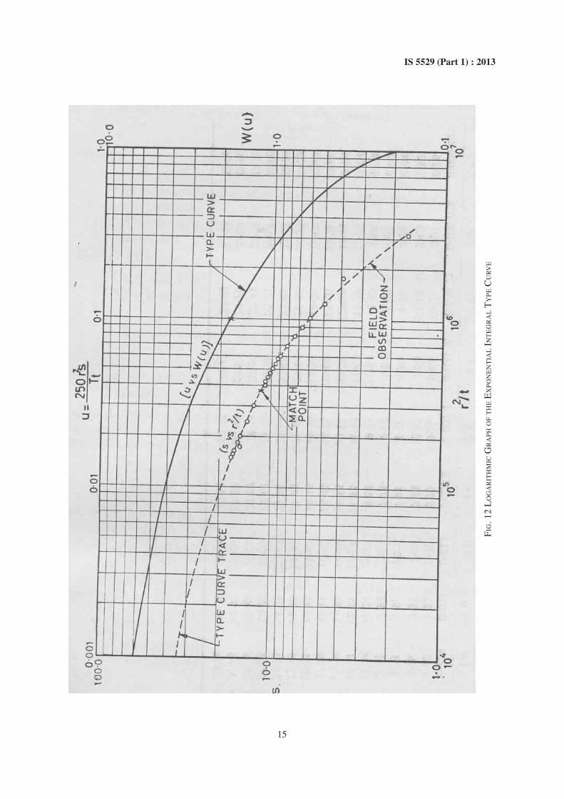
If in a test Rf, S and T are constant, the equations: (8)

and (9) indicate that s is related to r2/t in a manner that

is similar to the relation of W (u) to u. Consequently, if

values of drawdown s are plotted against r²/t on a

logarithmic paper to the same scale as W (u) versus u,

called the type curve, the curve of the observed field

data will be similar to the type curve. The plot of W (u)

versus u (see Fig. 12) is simply a graphical solution of

equation (8) and is plotted for reference. The values of

W(u) for values of u from 10 -15 to 9.0 (as tabulated by

Wenzel) are given in Table 2.

4.5.1.4 The graphical solution for T is as follows:

a) Plot the type curve W (u) versus u, using log

paper as shown by continuous line in Fig. 12.

The values of W (u) are taken from Table 2.

b) Plot the field data s versus r2/t using log paper

to the same scale as the type curve, shown by

circles in Fig. 12. (Either the type curve or

the field curve should be on transparent paper

for convenience in superimposing.)

c) Superimpose the two curves (transparent

curve is kept at the top) shifting laterally and

vertically but keeping the scale parallel to a

position which represents the best fit of the

field data to the type curve.

d) With both graph sheets at the best match

position, select an arbitrary point on the top

curve and mark on the lower curve.

15

IS 5529 (Part 1) : 2013

FIG

. 1

2 L

OG

AR

ITH

MIC

GR

AP

H O

F T

HE E

XP

ON

EN

TIA

L I

NT

EG

RA

L T

YP

E C

UR

VE

16

IS 5529 (Part 1) : 2013

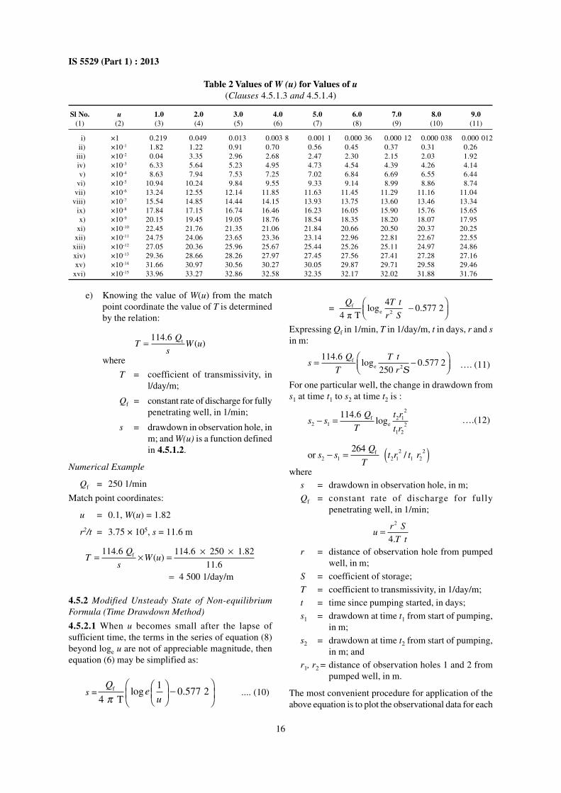
e) Knowing the value of W(u) from the match

point coordinate the value of T is determined

by the relation:

t114.6 ( )

QT W u

s=

where

T = coefficient of transmissivity, in

l/day/m;


penetrating well, in 1/min;

s = drawdown in observation hole, in

m; and W(u) is a function defined

in 4.5.1.2.

Numerical Example

Qf = 250 1/min

Match point coordinates:

u = 0.1, W(u) = 1.82

r2/t = 3.75 × 105, s = 11.6 m

f114.6 114.6 250 1.82( )

11.6

4 500 1/day/m

T W us

¥ ¥= ¥ =

=

Q

4.5.2 Modified Unsteady State of Non-equilibrium

Formula (Time Drawdown Method)

4.5.2.1 When u becomes small after the lapse of

sufficient time, the terms in the series of equation (8)

beyond loge u are not of appreciable magnitude, then

equation (6) may be simplified as:

s =f 1

log 0.577 24 T

Qe

uπ −

.... (10)

=�

fe 2

4 log 0.577 2

4 T

Q T t

r S

Ê ˆ-Á ˜Ë ¯

Expressing Qf in 1/min, T in 1/day/m, t in days, r and s

in m:

fe 2

114.6 log 0.577 2

250

Ts

T

Ê ˆ= -Á ˜Ë ¯Q t

r S…. (11)

For one particular well, the change in drawdown from

s1 at time t1 to s2 at time t2 is :

2

f 2 12 1 e 2

1 2

114.6 log

Q t rs s

T t r- = ….(12)

( )2 2f

2 1 2 1 1 2

264 or /

Qs s t r t r

T- =

where

s = drawdown in observation hole, in m;


penetrating well, in 1/min;

2

4.

r Su

T t=

r = distance of observation hole from pumped

well, in m;

S = coefficient of storage;

T = coefficient to transmissivity, in 1/day/m;

t = time since pumping started, in days;

s1 = drawdown at time t1 from start of pumping,

in m;

s2 = drawdown at time t2 from start of pumping,

in m; and

r1, r2 = distance of observation holes 1 and 2 from

pumped well, in m.

The most convenient procedure for application of the

above equation is to plot the observational data for each

Table 2 Values of W (u) for Values of u

(Clauses 4.5.1.3 and 4.5.1.4)

Sl No. u 1.0 2.0 3.0 4.0 5.0 6.0 7.0 8.0 9.0

(1) (2) (3) (4) (5) (6) (7) (8) (9) (10) (11)

i) ×1 0.219 0.049 0.013 0.003 8 0.001 1 0.000 36 0.000 12 0.000 038 0.000 012

ii) ×10-1 1.82 1.22 0.91 0.70 0.56 0.45 0.37 0.31 0.26

iii) ×10-2 0.04 3.35 2.96 2.68 2.47 2.30 2.15 2.03 1.92

iv) ×10-3 6.33 5.64 5.23 4.95 4.73 4.54 4.39 4.26 4.14

v) ×10-4 8.63 7.94 7.53 7.25 7.02 6.84 6.69 6.55 6.44

vi) ×10-5 10.94 10.24 9.84 9.55 9.33 9.14 8.99 8.86 8.74

vii) ×10-6 13.24 12.55 12.14 11.85 11.63 11.45 11.29 11.16 11.04

viii) ×10-7 15.54 14.85 14.44 14.15 13.93 13.75 13.60 13.46 13.34

ix) ×10-8 17.84 17.15 16.74 16.46 16.23 16.05 15.90 15.76 15.65

x) ×10-9 20.15 19.45 19.05 18.76 18.54 18.35 18.20 18.07 17.95

xi) ×10-10 22.45 21.76 21.35 21.06 21.84 20.66 20.50 20.37 20.25

xii) ×10-11 24.75 24.06 23.65 23.36 23.14 22.96 22.81 22.67 22.55

xiii) ×10-12 27.05 20.36 25.96 25.67 25.44 25.26 25.11 24.97 24.86

xiv) ×10-13 29.36 28.66 28.26 27.97 27.45 27.56 27.41 27.28 27.16

xv) ×10-14 31.66 30.97 30.56 30.27 30.05 29.87 29.71 29.58 29.46

xvi) ×10-15 33.96 33.27 32.86 32.58 32.35 32.17 32.02 31.88 31.76

17

IS 5529 (Part 1) : 2013

4.5.3 Analysis by Recovery Data

4.5.3.1 If a well that has been pumping for definite period

of time at a constant rate is shut down then recovery of

the water table takes place. The head distribution

thereafter is obtained by superimposing a recharge well

of the same strength as the discharge well, upon the

discharge well, to bring the net discharge to zero. The

residual drawdown s' (that is the difference at any time

between the static level and the recovering water level)

is the algebraic sum of the drawdown resulting from the

start-up and the recovery resulting from the shutdown

(assuming no leakage around the casing and neglecting

the volume of water that momentarily flows back into

the well from the pump column).

Thus

s' =�

f

2 2

2.30 2.25 2.25 log –log

4 T r S

Ê ˆÁ ˜Ë ¯

Q T t

r S

T t'

s' =p

f2.30 log / '

4

Qt t

T…(13)

where

s' = residual drawdown,


penetrating well,

well on semi log coordinate paper as shown in Fig. 13.

From this curve make an arbitrary choice of r12/t1 and

r22/t2 and note the corresponding values of s1 and s2.

For convenience r12/t1 and r2

2/t2 and are chosen one

log-cycle, apart, and then

( )2 2

10 1 2 2 1log / 1r t r t =

�

�

f

2 1

f

264 or

264 or

Qs s s

T

QT

s

- = =

=

where

s = drawdown difference per log cycle, in m.

Numerical Example

Qf = 250 1/min

r = 48 m

T =( )f 10 2 1

2 1

264 log /Q t t

s s-

or T =( )10264 250 log 100 /10

26.8 – 12.2

¥ ¥

or T = 4 520 1/day/m

FIG. 13 SEMI-LOG GRAPH OF PUMPING TEST DATA FOR APPLICATION OF MODIFIED THEIS FORMULA

18

IS 5529 (Part 1) : 2013

T = coefficient of transmissivity,

T = time elapsed since the start-up of pumping,

and

t' = time elapsed since shutdown of pump.

4.5.3.2 Measurements of residual drawdown, made

either in the well that has been pumped, or in a nearby

observation well, should be plotted against log (t/t')

and the coefficient of transmissivity T calculated again

from the slope of the straight line drawn through the

plotted point.

4.5.4 Unconfined Aquifer

4.5.4.1 The value of coefficient of transmissivity for

unconfined aquifer may be obtained from pump out

test by the formulae given in 4.5.1.1 to 4.5.1.3, if the

drawdown s is reduced by a factor

02

s

H

where

s = drawdown, and

H0 = natural or initial depth of flow.

4.5.4.2 It has been found that values obtained will be

fairly accurate, if the drawdowns are 25 percent of the

initial depth of flow and the storage coefficient is constant.

4.5.5 Theim’s Steady State or Equilibrium Method

4.5.5.1 When the well has run for sufficient length of

time and the drawdown cone has reached a state or

equilibrium, or steady flow condition over the entire

area of influence, the coefficient of transmissivity T

should be determined by Theim’s steady state formula

as follows:

( )�

f 2e

1 2 1

log2

Q rT

s s r=

- …. (14)

where

T = coefficient of transmissivity;

Qf = constant rate of discharge;

r1, r2 = distance of observation holes from the

pumping well as shown in Fig. 10; and

s1, s2 = drawdown in observation holes 1 and 2 as

shown in Fig. 10.

For unconfined aquifer:

( )f

e 2 12 2

2 1

log /Q

T r rh h

=−

… (15)

where


Qf = constant rate of discharge; and

h1, h2 = heads in observation holes 1 and 2.

5 PUMPING OUT TEST BY BAILOR METHOD

5.1 Applicability

The method is applicable to the approximate

determination of the permeability of the strata up to

shallow depth in the close vicinity of the well.

5.2 Equipment

5.2.1 Boring Set — One, of 200 mm to 250 mm.

5.2.2 Casing Pipe — To fit in the above hole with

strainer attached as in 4.2.4.

5.2.3 Bailor — One for bailing out water from the test

hole. The bailor may be a cylindrical bucket of 150 mm

dia and 0.3 m long attached with a 7 kg mass at the

bottom for sinking the bailor in the water. A rope is

tied on the top to facilitate the bailing out of water.

5.2.4 Equipment for Measuring Water Level in the Test

Hole

5.2.5 Miscellaneous Equipment — Tape, stop watch,

graduated cylinder and enamelled buckets.

5.3 Procedure

5.3.1 The boring of the hole, sinking the casing and

cleaning the hole should be done by the method

described in 3.2.3.1.

5.3.2 The water from the well should be bailed out for

the first bailor cycle and the time at which the water is

bailed out should be noted. The water level in the well

should be allowed to recover and the recovery after

arbitrary time t should be noted in the well itself. The

residual drawdown (static water level – recouped water

level) should also be noted. The process should be

repeated for a number of bailor cycles and the final

residual drawdown should be determined.

5.4 Computation of Coefficient of Transmissivity

5.4.1 When bailing of a well is stopped then at any

point on the recovery curve, the following equation

applies:

( )( )�2

w

'

4 . /4r

Vs

Tt e S Tt-

= .... (16)

where

s' = residual drawdown;

V = volume of water removed in one bailor cycle;


t = length of time since the bailor was removed;

rw = effective radius of the well; and

S = coefficient of storage.

19

IS 5529 (Part 1) : 2013

5.4.1.1 The effective radius rw of the well is very small

in comparison to the extent of the aquifer. As rw is small

the exponential term in equation (16) approaches to

unity as t becomes larger. Therefore, for large values

of t, the equation becomes (symbols same as in 5.4.1):

�'

4 12.57

V Vs

Tt Tt= =

5.4.1.2 If the residual drawdown is observed at some

time after completion of n bailor cycles, then the

following expression applies:

1 2 3 n

1 2 3 n

1' ...

12.57

V V V Vs

T t t t t

Ê ˆ= + + + +Á ˜Ë ¯

where, the subscripts merely identify each cycle of

events in sequence. Thus, V3 represents the volume of

water removed during the third bailor cycle and t3 is

the elapsed time from the instant that water was

removed from storage to the instant at which the

observation of residual drawdown was made.

5.4.1.3 If approximately the same volume of water V is

removed by the bailor during each cycle the equation

becomes:

s' =1 2 3 n

1 1 1 1 1...

12.57 T t t t t

Ê ˆ+ + + +Á ˜Ë ¯

or T =1 n

1

12.57 '

n n

ns t

=

=ÂV

where

n = number of bailing cycles.

5.4.1.4 Expressing V in litre, t in days, s' in m, then T is

expressed in 1/day/m.

5.4.2 The bailor method is applied to a single

observation of the residual drawdown after the time

since bailing stopped, becomes large. The

transmissivity is computed by substituting in equation,

the observed residual drawdown, the volume of water

V considered to be the average quantity removed by

the bailor in each cycle, and the summation of the

reciprocal of the elapsed time, in days, between the

time each bailor of water removed from the well and

time of observation of residual drawdown.

5.5 Observations



given in Annex E.

6 LIMITATIONS OF PUMPING OUT TESTS

6.1 It is a very uneconomical and cumbersome

method.

6.2 It does not give correct value of permeability for

stratified foundations.

6.3 Correct value of permeability is obtained only when

the well has been pumped for quite a long time and no

sand is coming out of the pumped well.

7 COMPUTATION FOR COEFFICIENT OF

PERMEABILITY

7.1 The coefficient of permeability K is computed from

the values of the coefficient of transmissivity by the

relation given below:K = T/b

expressing T in 1/day/m, b in m and K in m/day,

K = T/b × 10-3

where

K = coefficient of permeability in m/day;

T = coefficient of transmissivity in l/day/m; and

b = aquifer thickness in m.

7.2 The coefficient of permeability K may be expressed

in cm/s by the relation given below:

1 m/day = 1.157 × 10-3 cm/s

20

IS 5529 (Part 1) : 2013

ANNEX A

(Clause 3.2.4)

PROFORMA FOR RECORD OF OBSERVATIONS OF TEST BY CONSTANT HEAD METHOD

ANNEX B

(Clause 3.3.4)

PROFORMA FOR RECORD OF OBSERVATIONS OF TEST BY FALLING HEAD METHOD

Sl Time Elevation of H for Test Below Water H for Test Above Water

No. min Water Level Table = Elevation of Water Table = Elevation of Water Level

in the Casing Level in the Casing – Elevation in the Casing — Elevation

of Ground Water Table of the Test Section

(1) (2) (3) (4) (5)

i) 05

ii) 10

iii) 15

iv) 20

v) 25

Table for Discharge

Sl No. Discharge in Discharge

i)

ii)

iii)

1) Test No.:

2) Test location:

a) Elevation of ground:

b) Elevation of ground water table:

c) Elevation of the test section:

d) Diameter of test hole:

1) Test location:

2) Test No.:

3) Elevation of the ground:

4) Elevation of the ground water table:

5) Diameter of the intake pipe (d):

6) Length of the test section (L):

7) Water level at time t0 (h0):

21

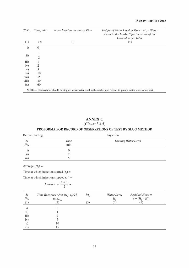
IS 5529 (Part 1) : 2013

Sl No. Time, min Water Level in the Intake Pipe Height of Water Level at Time t, H-t = Water

Level in the Intake Pipe-Elevation of the

Ground Water Table

(1) (2) (3) (4)

i) 0

ii)1

2

iii) 1

iv) 2

v) 5

vi) 10

vii) 15

viii) 30

ix) 60

NOTE — Observations should be stopped when water level in the intake pipe recedes to ground water table (or earlier).

ANNEX C

(Clause 3.4.5)

PROFORMA FOR RECORD OF OBSERVATIONS OF TEST BY SLUG METHOD

Before Starting Injection

Sl Time Existing Water Level

No. min

i) 0

ii) 2

iii) 5

Sl Time Recorded After [(t1+t

2)/2], 1/t

mWater Level Residual Head =

No. min, tm

H2

s = (H2 – H

1)

(1) (2) (3) (4) (5)

i) 0

ii) 1

iii) 2

iv) 5

v) 10

vi) 15

Average (H1) =

Time at which injection started (t1) =

Time at which injection stopped (t2) =

1 2 2

t tAverage

+= =

22

IS 5529 (Part 1) : 2013

ANNEX D

(Clause 4.4)

PROFORMA FOR RECORD OF OBSERVATIONS OF PUMPING OUT TESTS

Date:

1) Test location:

2) Test hole No.:

a) Diameter of the well:

b) Level of water table:

c) Thickness of saturated strata below water table:

d) Penetration of the well:

e) Length of strainer the well:

f) Length of top blind pipe of the well:

g) Length of strata tested (RL to RL):

h) Ground level:

DRAWDOWN OBSERVATIONS

Sl No. Time Line No. ( )Piezometer No. As per plan

1 2 3 4 5 6Well

��

i) 1

ii) 2

iii) 3

DISCHARGE OBSERVATIONS

(A) By Trajectory Method

Sl No. X Y V Amount of Seepage Qf

m1/min m1/min

(B) V-Notch Method

Sl No. Head of Water Discharge Qf

Over Notch ml/min

23

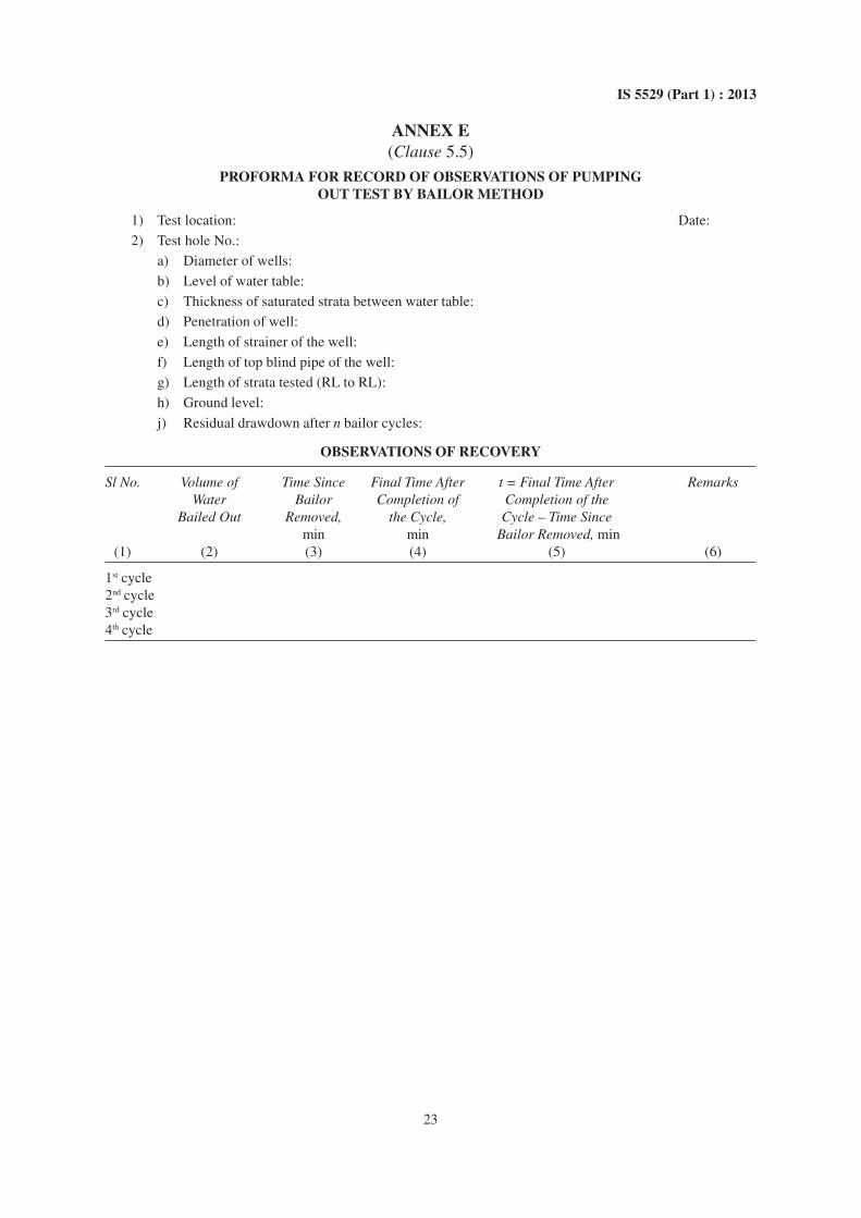
IS 5529 (Part 1) : 2013

ANNEX E

(Clause 5.5)

PROFORMA FOR RECORD OF OBSERVATIONS OF PUMPING

OUT TEST BY BAILOR METHOD

1) Test location: Date:

2) Test hole No.:

a) Diameter of wells:

b) Level of water table:

c) Thickness of saturated strata between water table:

d) Penetration of well:

e) Length of strainer of the well:

f) Length of top blind pipe of the well:

g) Length of strata tested (RL to RL):

h) Ground level:

j) Residual drawdown after n bailor cycles:

OBSERVATIONS OF RECOVERY

Sl No. Volume of Time Since Final Time After t = Final Time After Remarks

Water Bailor Completion of Completion of the

Bailed Out Removed, the Cycle, Cycle – Time Since

min min Bailor Removed, min

(1) (2) (3) (4) (5) (6)

1st cycle

2nd cycle

3rd cycle

4th cycle

Bureau of Indian Standards

BIS is a statutory institution established under the Bureau of Indian Standards Act, 1986 to promote

harmonious development of the activities of standardization, marking and quality certification of goods

and attending to connected matters in the country.

Copyright

BIS has the copyright of all its publications. No part of these publications may be reproduced in any form

without the prior permission in writing of BIS. This does not preclude the free use, in the course of

implementing the standard, of necessary details, such as symbols and sizes, type or grade designations.

Enquiries relating to copyright be addressed to the Director (Publications), BIS.

Review of Indian Standards

Amendments are issued to standards as the need arises on the basis of comments. Standards are also reviewed

periodically; a standard along with amendments is reaffirmed when such review indicates that no changes are

needed; if the review indicates that changes are needed, it is taken up for revision. Users of Indian Standards

should ascertain that they are in possession of the latest amendments or edition by referring to the latest issue of

‘BIS Catalogue’ and ‘Standards : Monthly Additions’.

This Indian Standard has been developed from Doc No.: WRD 5 (450).

Amendments Issued Since Publication

Amend No. Date of Issue Text Affected

BUREAU OF INDIAN STANDARDS

Headquarters:

Manak Bhavan, 9 Bahadur Shah Zafar Marg, New Delhi 110002

Telephones : 2323 0131, 2323 3375, 2323 9402 Website: www.bis.org.in

Regional Offices: Telephones

Central : Manak Bhavan, 9 Bahadur Shah Zafar Marg 2323 7617

NEW DELHI 110002 2323 3841

Eastern : 1/14 C.I.T. Scheme VII M, V. I. P. Road, Kankurgachi 2337 8499, 2337 8561

KOLKATA 700054 2337 8626, 2337 9120

Northern : SCO 335-336, Sector 34-A, CHANDIGARH 160022 60 3843

60 9285

Southern : C.I.T. Campus, IV Cross Road, CHENNAI 600113 2254 1216, 2254 1442

2254 2519, 2254 2315

Western : Manakalaya, E9 MIDC, Marol, Andheri (East) 2832 9295, 2832 7858

MUMBAI 400093 2832 7891, 2832 7892

Branches: AHMEDABAD. BANGALORE. BHOPAL. BHUBANESHWAR. COIMBATORE. DEHRADUN.

FARIDABAD. GHAZIABAD. GUWAHATI. HYDERABAD. JAIPUR. KANPUR. LUCKNOW.

NAGPUR. PARWANOO. PATNA. PUNE. RAJKOT. THIRUVANANTHAPURAM.

VISAKHAPATNAM.

�

��

�

�

Published by BIS, New Delhi

Is .5529.1.1985-Permeability Tests

Documents

Transcript of Is .5529.1.1985-Permeability Tests